Improving the Direct Determination of $|V_{ts}|$ using Deep Learning

Abstract

An $s$-jet tagging approach to determine the Cabibbo-Kobayashi-Maskawa matrix component $|V_{ts}|$ directly in the dileptonic final state events of the top pair production in proton-proton collisions has been previously studied by measuring the branching fraction of the decay of one of the top quarks by $\mathit{{t}{}_{\mspace{-3.0mu}\scriptstyle{}}^{\mspace{-1.0mu}\scriptstyle{}}}\to\mathit{{s}{}_{\mspace{-3.0mu}\scriptstyle{}}^{\mspace{-1.0mu}\scriptstyle{}}}\mathit{{W}{}_{\mspace{-3.0mu}\scriptstyle{}}^{\mspace{-1.0mu}\scriptstyle{}}}$. The main challenge is improving the discrimination performance between strange jets from top decays and other jets. This study proposes novel jet discriminators, called DiSaJa, using a Transformer-based deep learning method. The first model, DiSaJa-H, utilizes multi-domain inputs (jets, leptons, and missing transverse momentum). An additional model, DiSaJa-L, further improves the setup by using lower-level jet constituent information, rather than the high-level clustered information. DiSaJa-L is a novel model that combines low-level jet constituent analysis with event classification using multi-domain inputs. The model performance is evaluated via a CMS-like LHC Run 2 fast simulation by comparing various statistical test results to those from a model based on boosted decision trees. This study shows the deep learning model has a significant performance gain over the traditional machine learning method, and we show the potential of the measurement during Run 3 of the LHC and HL-LHC.

I Introduction

The Cabibbo-Kobayashi-Maskawa (CKM) matrix is the $3\times 3$ unitary complex matrix that gives the strength of the charged-current weak interaction between the quark generations in the Standard Model (SM) [1]. A global fit has been performed to constrain its components using measurements of various aspects of the CKM matrix and by imposing the SM condition of unitarity [2]. Although the fit gives precise values for each CKM component, further measurements are necessary to test the validity of the unitarity condition. In particular, the unitarity is no longer valid in several beyond the SM (BSM) theories [3]. Therefore, direct measurement of the components should be performed to test the SM consistency and constrain BSM scenarios.

In this paper, we focus on the measurement potential of the third-row component $|V_{ts}|$, whose squared value gives the branching ratio of the decay of the top quark to the strange quark and a $W$ boson in the SM. In the global fit of the CKM under the SM conditions, the value of $|V_{ts}|$ is $4.110^{+0.083}_{-0.072}\times 10^{-2}$ [2]. There have been several studies for measuring the component indirectly, which are used in the global fit. For example, $|V_{ts}|$ is determined indirectly using the $\mathit{{B}{}_{\mspace{-3.0mu}\scriptstyle{\mathit{{s}{}_{\mspace{-3.0mu}\scriptstyle{}}^{\mspace{-1.0mu}\scriptstyle{}}}}}^{\mspace{-1.0mu}\scriptstyle{0}}}-\mathit{{\mkern 4.0mu\overline{\mkern-4.0mu{B}}}{}_{\mspace{-2.0mu}\scriptstyle{\mathit{{s}{}_{\mspace{-3.0mu}\scriptstyle{}}^{\mspace{-1.0mu}\scriptstyle{}}}}}^{\mspace{0.0mu}\scriptstyle{0}}}$ oscillation frequency [4, 5, 6] and decay constant parameters from lattice QCD results [7], which results in $|V_{ts}|=4.15\pm 0.09\times 10^{-2}$ [2]. However, as the indirect measurements rely on loop processes, there could be BSM contributions and therefore these measurements could yield results that differ from the true value of $|V_{ts}|$. For example, BSM models with additional quark generations allow $|V_{ts}|$ to be as large as 0.2 [3].

There are several measurements for the model-independent direct determination of the $V_{tx}$ components, where $x$ is $\mathit{{d}{}_{\mspace{-3.0mu}\scriptstyle{}}^{\mspace{-1.0mu}\scriptstyle{}}}$, $\mathit{{s}{}_{\mspace{-3.0mu}\scriptstyle{}}^{\mspace{-1.0mu}\scriptstyle{}}}$, and $\mathit{{b}{}_{\mspace{-3.0mu}\scriptstyle{}}^{\mspace{-1.0mu}\scriptstyle{}}}$. For instance, a recent analysis with the CMS 13 TeV data with the single top process probes the $tWq$ vertices in production and decay in the $t$-channel. The study gives limits of $|V_{ts}|+|V_{td}|<0.057$ and $|V_{ts}|+|V_{td}|<0.06$ at the 95% confidence level (CL) under SM CKM unitarity and after relaxing the SM constraint, respectively [8]. Additionally, previous studies have proposed the direct determination using a light-flavor jet tagging approach to discriminate strange jets from the $\mathit{{t}{}_{\mspace{-3.0mu}\scriptstyle{}}^{\mspace{-1.0mu}\scriptstyle{}}}\to\mathit{{s}{}_{\mspace{-3.0mu}\scriptstyle{}}^{\mspace{-1.0mu}\scriptstyle{}}}\mathit{{W}{}_{\mspace{-3.0mu}\scriptstyle{}}^{\mspace{-1.0mu}\scriptstyle{}}}$ decay in the top pair production process for $|V_{ts}|$ [9, 10] or the $\mathit{{b}{}_{\mspace{-3.0mu}\scriptstyle{}}^{\mspace{-1.0mu}\scriptstyle{}}}$-jets from $t\to bW$ for $|V_{tb}|$ [11].

In this study, we expand on the jet tagging strategy for measuring $|V_{ts}|$ using a Deep Learning (DL) approach. The direct $s$-tagging approach is challenging due to the lack of statistics for signal events from $\mathit{{t}{}_{\mspace{-3.0mu}\scriptstyle{}}^{\mspace{-1.0mu}\scriptstyle{}}}\to\mathit{{s}{}_{\mspace{-3.0mu}\scriptstyle{}}^{\mspace{-1.0mu}\scriptstyle{}}}\mathit{{W}{}_{\mspace{-3.0mu}\scriptstyle{}}^{\mspace{-1.0mu}\scriptstyle{}}}$ compared to $t\to bW$, which is the most dominant background process, as the ratio of the signal to the background decay is given by $\frac{|V_{tb}|^{2}}{|V_{ts}|^{2}}\simeq 590$. Consequently, improving the separation power between the signal and background jets is crucial.

We propose a novel method to separate strange jets originating from top decays, starting from a self-attention-based network, SaJa [12], originally developed for the assignment of jets to partons in the $t\bar{t}$ all-hadronic channel, where large QCD multijet backgrounds dominate the analysis. We extend the SaJa model to apply to the dilepton channel events of top pair production, and we call these new models DiSaJa. Using the dileptonic channel, there are fewer background jets in each event, due to the reduced jet activity in an event compared to the other top pair decay channels. To reflect the diverse decay products in the dilepton channel, DiSaJa-H employs dedicated embedding networks for leptons, jets, and missing energy to process all the reconstructed physics objects in an event.

Numerous studies [13, 14, 15, 16] have reported that DL models using jet constituents as inputs demonstrate outstanding performance in object-level tasks such as flavor tagging. However, for event-level tasks, such as signal-background discrimination and jet-parton assignment, the representation of input jets has been restricted to the format of high-level feature variables rather than their constituents [12, 17, 18]. In this study, we produce an additional model, DiSaJa-L, which replaces the jet embedding layer in DiSaJa-H with a dedicated embedding network that processes jet constituents as inputs, enabling the model to learn jet representations optimized for this analysis. DiSaJa-L is thus a new general-purpose model that incorporates both low-level jet constituent analysis and multi-domain inputs, able to process the complete information available in hadron collider data.

This paper is organized as follows. Section II describes the event generation and detector simulation used in our analysis. In Section III, we present the object and event selection criteria. In Section IV, we explain the DL methods we use in this paper. As well as explaining the DiSaJa networks, we also consider a boosted decision trees (BDT) model, which was used in the previous $|V_{ts}|$ measurement proposals, as a baseline for evaluating the performance improvement of the DiSaJa models. In Section V, we compare the model performance for the $|V_{ts}|$ measurement between two DiSaJa models and the baseline BDT model with the simulated dataset. We also check the sensitivity of the measurement expected from the Run 3 and High-Luminosity LHC (HL-LHC) experiments [19] for evaluating the prospect of analyses performed at other integrated luminosities.

II Simulation settings

We generate $t\bar{t}$ dilepton channel events with up to two additional partons in $pp$ collisions at $\sqrt{s}=$13\text{\,}\mathrm{T\text{e\kern-0.6458ptV}}$$ at next-to-leading order (NLO) in QCD using MadGraph5_aMC@NLO 2.6.5 [20] with NNPDF 3.1 [21]. The signal process is $t\bar{t}$ where one $t$ quark decays to a $\mathit{{s}{}_{\mspace{-3.0mu}\scriptstyle{}}^{\mspace{-1.0mu}\scriptstyle{}}}$ quark ($t\bar{t}\to sWbW$) while the background is $t\bar{t}$, where both $\mathit{{t}{}_{\mspace{-3.0mu}\scriptstyle{}}^{\mspace{-1.0mu}\scriptstyle{}}}$ quarks decay to $\mathit{{b}{}_{\mspace{-3.0mu}\scriptstyle{}}^{\mspace{-1.0mu}\scriptstyle{}}}$ quarks ($t\bar{t}\to bWbW$) and the number of events generated for each process is about 50M. The inclusive $t\bar{t}$ cross section for $\sqrt{s}=13$ TeV is calculated to be $831.76\text{\,}\mathrm{pb}$, which is obtained at the next-to-next-to-leading order (NNLO) QCD and next-to-next-to-leading-logarithmic (NNLL) soft-gluon resummation with Top++ [22]. We take the cross sections of dileptonic $t\bar{t}\to sWbW$ and $t\bar{t}\to bWbW$ to be $0.337\text{\,}\mathrm{pb}$ and $88.99\text{\,}\mathrm{pb}$, respectively, by using the values of the inclusive cross section, the branching ratio of $\mathit{{W}{}_{\mspace{-3.0mu}\scriptstyle{}}^{\mspace{-1.0mu}\scriptstyle{}}}\to\mathit{{\ell}{}_{\mspace{-3.0mu}\scriptstyle{}}^{\mspace{-1.0mu}\scriptstyle{}}}\mathit{{\nu}{}_{\mspace{-3.0mu}\scriptstyle{}}^{\mspace{-1.0mu}\scriptstyle{}}}$ ($\mathit{{\ell}{}_{\mspace{-3.0mu}\scriptstyle{}}^{\mspace{-1.0mu}\scriptstyle{}}}=\mathit{{e}{}_{\mspace{-3.0mu}\scriptstyle{}}^{\mspace{-1.0mu}\scriptstyle{}}},\mathit{{\mu}{}_{\mspace{-3.0mu}\scriptstyle{}}^{\mspace{-1.0mu}\scriptstyle{}}},\mathit{{\tau}{}_{\mspace{-3.0mu}\scriptstyle{}}^{\mspace{-1.0mu}\scriptstyle{}}}$), $V_{ts}$, and $V_{tb}$ [2]. While the most dominant background is the $t\bar{t}\to bWbW$, there are also non-negligible backgrounds from non-$t\bar{t}$ processes such as single top (ST), Drell-Yan (DY), and diboson (VV) production. The ST $t$-channel and $tW$-associated processes with no additional partons and DY events with two additional partons in the final state ($DY+jj$) are generated at the NLO accuracy in QCD using MadGraph5_aMC@NLO 2.6.5 [20] with NNPDF 3.1 [21] and the generated number of events is about 220M, 220M, and 250M, respectively. In the ST generation, $\mathit{{W}{}_{\mspace{-3.0mu}\scriptstyle{}}^{\mspace{-1.0mu}\scriptstyle{}}}$ boson is forced to decay leptonically for more efficient event generation. For the generation of the DY process, the invariant mass of final state lepton pair is set to be greater than $50\text{\,}\mathrm{G\text{e\kern-0.6458ptV}}$. The $VV$ processes ($WW$, $WZ$, and $ZZ$) are generated as about 20M events for each process using Pythia 8.240 [23] and their cross sections are set to $118.7\text{\,}\mathrm{pb}$ [24], $49.98\text{\,}\mathrm{pb}$ [25], and $16.91\text{\,}\mathrm{pb}$ [26], respectively, at the NNLO in QCD.

After the matrix element level event generation, parton showering and hadronization are simulated with Pythia 8. The matrix element events are jet-matched with the parton shower using the FxFx scheme [27] and the CP5 tuning parameters are used for modeling the underlying event [28]. After the simulation, the cross sections of the ST $t$-channel, the $tW$-associated, and the DY are obtained as 73.45, 3.289, and $359.1\text{\,}\mathrm{pb}$, respectively.

We use Delphes 3.4.2 [29] to simulate the response of a CMS-like detector. Delphes takes outputs from Pythia 8 and emulates the propagation of the particles in the magnetic field and the response of the particles in the detector’s tracker and calorimeters. Using this information, Delphes produces reconstructed charged particle tracks (tracks) and neutral particles’ energy depositions in the calorimeters (towers). These objects are used for reconstructing high-level objects, which are the isolated leptons and the jets made from clustering the tracks and towers. The kinematics of the tracks and towers objects are also summed and the transverse component of the result is negated to produce the missing transverse momentum ($\vec{p_{T}}^{miss}$ or MET) of the event. We change the default Delphes CMS card to reflect the Run 2 conditions by using update values for the $\Delta R$ for the lepton isolation, the jet clustering radius, and the $\mathit{{b}{}_{\mspace{-3.0mu}\scriptstyle{}}^{\mspace{-1.0mu}\scriptstyle{}}}$-tagging efficiency. The $\Delta R$ for lepton isolation is set to 0.3 (0.4) for electrons (muons). The anti-$k_{T}$ algorithm is used for jet clustering with the jet radius $R=0.4$ using FastJet 3.3.2 [30], and the $b$-tagging efficiency is updated based on the efficiency distribution used by the CMS experiment [31, 32]. To emulate tracks in the CMS tracker, the track impact parameter is smeared and the resolution of the track transverse momentum is applied based on a CMS tracker performance study [33].

III Event selection

This analysis is performed with top pair production in the dilepton $ee$, $e\mu$, and $\mu\mu$ channels. We identify $t\bar{t}$ dilepton events using the standard selection criteria found in various CMS top analyses [34, 35, 36]. Charged leptons are selected using a cone-based relative isolation $I_{rel}$ [29], and kinematic requirements. For muons, the isolation is required to be $I_{rel}<0.15$ while electrons are selected when $I_{rel}<0.0588\ (0.0571)$ in the barrel (endcap) region. Both flavors of lepton are required to be within $|\eta|<2.4$, but electrons in the ECAL transition gap region $1.44<|\eta|<1.57$ are excluded [37]. We select jets with $p_{T}>30$ GeV and $|\eta|<2.4$, vetoing jets where the distance from a selected lepton $\Delta R$ is less than 0.4. Among the remaining selected jets, jets are $b$-tagged according to the CMS $\mathit{{b}{}_{\mspace{-3.0mu}\scriptstyle{}}^{\mspace{-1.0mu}\scriptstyle{}}}$-tagging efficiency parameterized as a function $p_{T}$ and $\eta$.

We select events with exactly one lepton pair with opposite charges where the invariant mass $M_{\mathit{{\ell}{}_{\mspace{-3.0mu}\scriptstyle{}}^{\mspace{-1.0mu}\scriptstyle{}}}\mathit{{\ell}{}_{\mspace{-3.0mu}\scriptstyle{}}^{\mspace{-1.0mu}\scriptstyle{}}}}$ of the lepton pair is required to be greater than $20\text{\,}\mathrm{G}\mathrm{e}\mathrm{V}$, and the $p_{T}$ of the leading (subleading) lepton is required to be greater than 25 (20) GeV. For the same-flavor (SF) channel, we require $|M_{ll}-M_{\mathit{{Z}{}_{\mspace{-3.0mu}\scriptstyle{}}^{\mspace{-1.0mu}\scriptstyle{}}}}|>$15\text{\,}\mathrm{G\text{e\kern-0.6458ptV}}$$, where the mass of $\mathit{{Z}{}_{\mspace{-3.0mu}\scriptstyle{}}^{\mspace{-1.0mu}\scriptstyle{}}}$ boson $M_{\mathit{{Z}{}_{\mspace{-3.0mu}\scriptstyle{}}^{\mspace{-1.0mu}\scriptstyle{}}}}\simeq 91$ GeV [2], to veto the $\mathit{{Z}{}_{\mspace{-3.0mu}\scriptstyle{}}^{\mspace{-1.0mu}\scriptstyle{}}}$ boson background. Additionally, for the SF channel, we require that the missing transverse momentum $p_{T}^{miss}>40$ GeV. We use events with at least two selected jets, where at most one jet is $b$-tagged.

We refer to jets originating from the parton $\mathit{{q}{}_{\mspace{-3.0mu}\scriptstyle{}}^{\mspace{-1.0mu}\scriptstyle{}}}$ in top quark decays $\mathit{{t}{}_{\mspace{-3.0mu}\scriptstyle{}}^{\mspace{-1.0mu}\scriptstyle{}}}\to\mathit{{q}{}_{\mspace{-3.0mu}\scriptstyle{}}^{\mspace{-1.0mu}\scriptstyle{}}}\mathit{{W}{}_{\mspace{-3.0mu}\scriptstyle{}}^{\mspace{-1.0mu}\scriptstyle{}}}$ as primary jets. Consequently, the signal jet is called the primary $\mathit{{s}{}_{\mspace{-3.0mu}\scriptstyle{}}^{\mspace{-1.0mu}\scriptstyle{}}}$ jet in this paper. Primary jets are identified as reconstructed jets matched to generator-level quarks from top quark decays. Matching is performed by requiring the distance $\Delta R$ between the parton and the jet satisfies $\Delta R<0.4$. If there exist multiple $\Delta R$-matched jets, which occur in less than 1% of signal events, the jet having the highest $p_{T}$ is identified as the primary jet. In 85% of signal events, there is a jet matched to the $\mathit{{t}{}_{\mspace{-3.0mu}\scriptstyle{}}^{\mspace{-1.0mu}\scriptstyle{}}}\to\mathit{{s}{}_{\mspace{-3.0mu}\scriptstyle{}}^{\mspace{-1.0mu}\scriptstyle{}}}\mathit{{W}{}_{\mspace{-3.0mu}\scriptstyle{}}^{\mspace{-1.0mu}\scriptstyle{}}}$ parton.

IV Machine learning

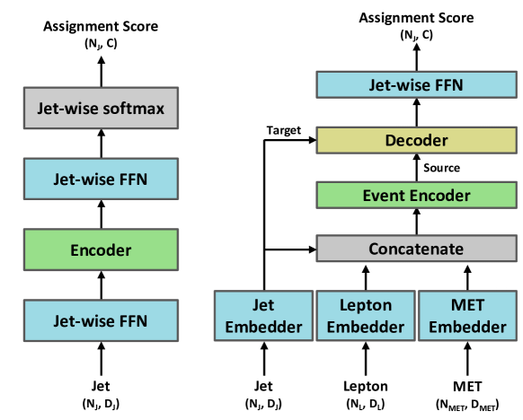
Figure 1: Architecture of the original SaJa model (left) and the DiSaJa-H (right). $N_{x}$, $D_{x}$, and C denote the number of the object $x\in$ {jets, leptons, MET}, the dimension size of the object $x$, and the number of output categories, respectively.

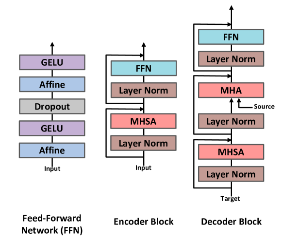
Figure 2: Detailed network structure of blocks of Feed-Forward Network, Encoder, and Decoder. The decoder processes the output of the jet embedder as the target input and the output of the event encoder block as the source input.

The original SaJa model, illustrated in Fig. 1, is designed for the task of jet assignment in fully hadronic top pair production and is built upon the Transformer encoder architecture [38]. It processes high-level jet features using a combination of Feed-Forward Networks (FFN) and a Transformer encoder block, which is displayed in Fig. 2. The FFN block consists of two layers of affine transformations, each followed by a Gaussian Error Linear Unit (GELU) activation function [39], with dropout applied to prevent overfitting [40]. The array of jet vectors is passed through the jet-wise FFN blocks. The encoder block, detailed below, allows for the interaction between the jet arrays through the use of the self-attention mechanism.

Generically, attention is a function that takes a source $\mathbf{S}\in\mathbb{R}^{M\times D_{S}}$ and a target $\mathbf{T}\in\mathbb{R}^{N\times D_{T}}$ as input and produces an output array of the same length as the target, where $M$ and $N$ are the lengths of arrays and each element in $\mathbf{S}$ ($\mathbf{T}$) is a vector of dimension $D_{S}$ ($D_{T}$). The purpose of attention is to transform $\mathbf{T}$ into a rich contextual representation by extracting and integrating relevant information from $\mathbf{S}$; we say that $\mathbf{T}$ attends to $\mathbf{S}$. First, $\mathbf{T}$ is projected into $\mathbf{Q}\in\mathbb{R}^{N\times D_{K}}$, and $\mathbf{S}$ is projected into $\mathbf{K}\in\mathbb{R}^{M\times D_{K}}$ and $\mathbf{V}\in\mathbb{R}^{M\times D_{V}}$ using separate affine transformations. $\mathbf{Q}$, $\mathbf{K}$, and $\mathbf{V}$ are then passed through scaled dot-product attention function:

$$\text{Attention}\left(\mathbf{Q},\mathbf{K},\mathbf{V}\right)=\text{softmax}\left(\frac{\mathbf{Q}\mathbf{K}^{T}}{\sqrt{D_{K}}}\right)\mathbf{V}\in\mathbb{R}^{N\times D_{V}},$$ (1)

where softmax is applied to each row of the output of scaled dot-product attention. Self-attention is a special case of attention where $\mathbf{S}=\mathbf{T}$. That is, a single set of objects attends to itself.

In the encoder block, multi-head self-attention (MHSA) is used, which is a concatenation of $N_{\textrm{head}}$ copies of the scaled-dot product attention described above. The encoder is comprised of $N_{\textrm{block}}$ encoder blocks run sequentially, where each block consists of an MHSA block followed by an FFN block. The output of these blocks is added residually to the input arrays.

Object	Variable	Definition
Jet	$p_{T}(j),\eta(j),\phi(j),M(j)$	Momentum components of jet
	$N_{h^{0}}$	Neutral hadron multiplicity
	$N_{h^{\pm}}$	Charged hadron multiplicity
	$N_{e}$	Electron multiplicity
	$N_{\mu}$	Muon multiplicity
	$N_{P}$	Photon multiplicity
	$p_{T}$D	Jet energy sharing
	Jet axes	Lengths of ellipse
	Jet b tag	Boolean indicating whether a jet is b-tagged or not
	Jet charge	Jet charge
Lepton	$p_{T}(\ell),\eta(\ell),\phi(\ell),M(\ell)$	Momentum components of lepton
	Lepton flavor	0 for e, 1 for $\mu$
	$Q_{\ell}$	Lepton charge
MET	$p_{T}^{miss}$, $\phi(p_{T}^{miss})$	Magnitude and azimuth angle of $\vec{p_{T}}^{miss}$

Table 1: Features used as inputs in the models for each object type (jet, lepton, and MET). The BDT applies a jet-wise approach, whereas DiSaJa-H processes them event-wise.

Unlike the original SaJa, the DiSaJa-H is designed to process multi-domain inputs to utilize all of the objects in the dilepton final state events effectively. Fig. 1 presents an overview of the DiSaJa-H architecture, including input embedding networks (or embedders), event encoder, decoder, and jet-wise classification head blocks. In the initial step, input features listed in Table 1 for each object (reconstructed jet, lepton, and MET) are embedded into the same dimensional space through each FFN block. The momentum components of the jet, the number of particles in the jet (for each category of particle), the jet energy sharing ($p_{T}D=\frac{\sqrt{\sum_{i}{p_{T,i}^{2}}}}{\sum_{i}{p_{T,i}}}$, where $i$ indexes over particles inside jet) [41, 42], the jet shape, the jet $b$ tagging information, and the jet charge ($Q_{\kappa}=\sum_{h\in jet}z_{h}^{\kappa}Q_{h}$, where $z_{h}=p_{T_{h}}/p_{T_{jet}}$, $\kappa=0.3$) [43, 44, 45] are used as inputs to the jet array. For leptons, the momentum components, flavor, and charge are used. For the missing transverse momentum, its magnitude and azimuth angle are used as inputs. All input features are scaled to a range between 0 and 1 using min-max scaling. In DiSaJa-H, the separate object embedders allow different objects to be concatenated in a sequence by projecting them into the same dimensional space and they are then processed together by the event encoder, as in the original SaJa model. The encoder is followed by the decoder, which uses the Transformer decoder architecture, and which takes the jet embedder’s output as the target input and the event encoder’s output as the source input. The MHSA block first processes the jet embedding input, and the output is combined with the event encoder output using multi-head attention to integrate the full event information into each jet vector. The output of the decoder is passed to the jet-wise classification head, which assigns categorical scores for jets in each event using the final FFN head.

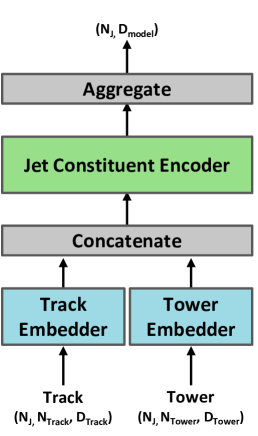
Figure 3: Architecture of the jet constituent encoder, which can replace the jet high-level feature encoder. Track and tower features are fed into encoders and the jet constituent encoder learns jet representation.

Variable	Definition
$p_{T}(P),\eta(P),\phi(P)$	Momentum components of particle
$\Delta\eta$	Difference of pseudorapidity between particle and jet axis
$\Delta\phi$	Difference of azimuthal angle $\phi$ between particle and jet axis
$\frac{p_{T}(P)}{p_{T}(j)}$	$p_{T}$ of a constituent relative to jet $p_{T}$
$p_{T}^{rel}$	Particle momentum perpendicular to the jet axis
$p_{z}^{rel}$	Particle momentum in the direction of jet axis
$d_{0}$	Transverse track impact parameter value
$d_{z}$	Longitudinal track impact parameter value
$Q_{P}$	Charge of particle
$E_{EM}$, $E_{had}$	Electromagnetic, hadronic energy in calorimeter

Table 2: Input features of jet constituents

The DiSaJa-L model starts from the DiSaJa-H model as a base, and is augmented by utilizing arrays of jet constituent information as inputs instead of the high-level jet variables produced after the jet clustering. The low-level jet embedder is thus a drop-in replacement of the high-level jet embedder. Fig. 3 shows the architecture of the low-level jet embedder, which is designed to extract the informative representations of jets from their constituents, which are the tracks and towers produced by Delphes. The input feature variables of tracks and towers are summarized in Table 2. To address these differences, the low-level jet embedder includes two separate FFNs, which project tracks and towers into the same dimension, and are called the track and tower embedders, respectively. The outputs of track and tower embedders are then concatenated and passed into a jet constituent encoder, which also uses the Transformer encoder architecture described above. Then, the aggregate block averages the output of the jet constituent encoder over the constituent axis to produce a single vector per jet, which is used in the rest of the model, as in DiSaJa-H.

For the training and validation, we use a selected subsample of the generated $t\bar{t}\to sWbW$ and $t\bar{t}\to bWbW$ events. For training, we use around 1.1M events, which are required to contain $\mathit{{t}{}_{\mspace{-3.0mu}\scriptstyle{}}^{\mspace{-1.0mu}\scriptstyle{}}}\to\mathit{{s}{}_{\mspace{-3.0mu}\scriptstyle{}}^{\mspace{-1.0mu}\scriptstyle{}}}\mathit{{W}{}_{\mspace{-3.0mu}\scriptstyle{}}^{\mspace{-1.0mu}\scriptstyle{}}}$ jet-parton matched jet, with no requirement of a $t\to bW$ matched jet. In the case of the background sample, we use about 0.5M events where both $t\to bW$ partons have jet matches and 0.4M events of unmatched events, where at least one of the $t\to bW$ jet-parton matches is missing. For model selection, we use around 275K signal events and 221K (121K of matched and 100K unmatched) background events, passing the same matching requirements but chosen separately from the training samples, as the validation dataset.

The models are trained to classify jets into three groups: $\mathit{{t}{}_{\mspace{-3.0mu}\scriptstyle{}}^{\mspace{-1.0mu}\scriptstyle{}}}\to\mathit{{s}{}_{\mspace{-3.0mu}\scriptstyle{}}^{\mspace{-1.0mu}\scriptstyle{}}}\mathit{{W}{}_{\mspace{-3.0mu}\scriptstyle{}}^{\mspace{-1.0mu}\scriptstyle{}}}$, $t\to bW$, and other jets, which represent the jet categories of interest in the signal process $t\bar{t}\to sWbW$. The models are provided with MC truth labels for the jet category of each jet in an event during training. We use jet-wise cross entropy as the objective function $L$ for training, which is defined for each event as follows:

$$L(\theta)=\frac{1}{N}\sum\limits_{j=1}^{N}\left(-\sum_{c\in\mathbb{C}}y_{c}^{(j)}\log\hat{y}_{c}^{(j)}\right)$$ (2)

where $\theta$ denotes the adjustable parameters of a model, $N$ is the number of jets in the event, $j$ indexes over the jets in the events, $c$ indexes over the jet categories $\mathbb{C}=\{\mathit{{t}{}_{\mspace{-3.0mu}\scriptstyle{}}^{\mspace{-1.0mu}\scriptstyle{}}}\to\mathit{{s}{}_{\mspace{-3.0mu}\scriptstyle{}}^{\mspace{-1.0mu}\scriptstyle{}}}\mathit{{W}{}_{\mspace{-3.0mu}\scriptstyle{}}^{\mspace{-1.0mu}\scriptstyle{}}},t\to bW,\text{other}\}$, $y_{c}^{(j)}$ is 1 for the true jet category $c$ for jet $j$ and 0 otherwise, and $\hat{y}_{c}^{(j)}=\hat{y}_{c}^{(j)}(\theta)$ is the model output for the jet $j$ in category $c$. Model optimization is performed with the AdamW optimizer [46] with $\beta_{1}=0.9$, $\beta_{2}=0.999$, a learning rate of 0.0003, and a weight decay coefficient of 0.01. We use mini-batch training, where each batch consists of 128 randomly sampled events for each training iteration. To handle variable-length jets and their constituents, input variables are zero-padded to match the maximum length of inputs within a batch, allowing us to use all the jets in each event without truncation. We evaluate the loss on the validation set during training and hyperparameter optimization and select the model with the lowest loss.

While we train models to classify all the jets of the $t\bar{t}\to sWbW$ signal process, DiSaJa’s output scores should also effectively discriminate signal events against background events. Further, since the difference between the $t\bar{t}\to sWbW$ signal process and the main background $t\bar{t}\to bWbW$ is the presences of the $\mathit{{t}{}_{\mspace{-3.0mu}\scriptstyle{}}^{\mspace{-1.0mu}\scriptstyle{}}}\to\mathit{{s}{}_{\mspace{-3.0mu}\scriptstyle{}}^{\mspace{-1.0mu}\scriptstyle{}}}\mathit{{W}{}_{\mspace{-3.0mu}\scriptstyle{}}^{\mspace{-1.0mu}\scriptstyle{}}}$ jet, we use the highest $\mathit{{t}{}_{\mspace{-3.0mu}\scriptstyle{}}^{\mspace{-1.0mu}\scriptstyle{}}}\to\mathit{{s}{}_{\mspace{-3.0mu}\scriptstyle{}}^{\mspace{-1.0mu}\scriptstyle{}}}\mathit{{W}{}_{\mspace{-3.0mu}\scriptstyle{}}^{\mspace{-1.0mu}\scriptstyle{}}}$ score within each event as a signal-background discriminant and the corresponding jet is referred to as the predicted primary $\mathit{{s}{}_{\mspace{-3.0mu}\scriptstyle{}}^{\mspace{-1.0mu}\scriptstyle{}}}$ jet. However, we found that models trained on only signal events, while achieving good assignment performance, showed limited discrimination power between signal and background events. This challenge arises because the $t\bar{t}\to bWbW$ background process shares the same event topology with the $t\bar{t}\to sWbW$ signal, and other background processes can also mimic it. Because the $t\bar{t}\to bWbW$ background is statistically dominant after the final event selection, we explore incorporating $t\bar{t}\to bWbW$ background events into the training set. The impact of these different training configurations is evaluated by comparing the significance of excluding $|V_{ts}|=0$, assuming an integrated luminosity of $138$ fb^-1. The precise definition of the significance is given in Sec. V.

First, we train a DiSaJa-H model using the signal-only training set, which contains only jet-parton matched $t\bar{t}\to sWbW$ events and constructs a baseline for the different training set configurations. The signal-only training set model achieves a significance of 2.94$\sigma$. The second configuration is based on a training set comprising both matched $t\bar{t}\to sWbW$ signal events and matched $t\bar{t}\to bWbW$ background events. Jets in matched $t\bar{t}\to bWbW$ events are labeled using jet-parton matching information as for $t\bar{t}\to sWbW$ events. The result with this configuration yields a significance of 3.44$\sigma$, demonstrating improved discrimination between signal and background. The training set for the final configuration also includes the unmatched $t\bar{t}\to bWbW$, and for these events all jets are labeled as other jets. This approach results in a significance of 4.29$\sigma$, the highest among the tested configurations. Based on these results, we use the final training configuration for the results of this study.

We optimize the hyperparameters of the DiSaJa-H model using the tree-structured Parzen estimator algorithm [47] within the Optuna framework [48]. The same hyperparameters are applied to DiSaJa-L. The hyperparameters for the model are $D_{\textrm{FFN}}$, $N_{\textrm{block}}$, $N_{\textrm{head}}$, and $D_{\textrm{model}}$, where $D_{\textrm{model}}$ is $N_{\textrm{head}}$ $\times$ dimension of each attention in MHSA, and are determined to be 1024, 2, 12, and 384, respectively.

The DiSaJa models are compared with a BDT model as a baseline. We implement the BDT model using the XGBoost (eXtreme Gradient Boosting) library [49]. The BDT model is configured with a learning rate of 0.3, a maximum tree depth of 6, and an L2 regularization weight of 1. The BDT is trained to classify each jet into three categories: $\mathit{{t}{}_{\mspace{-3.0mu}\scriptstyle{}}^{\mspace{-1.0mu}\scriptstyle{}}}\to\mathit{{s}{}_{\mspace{-3.0mu}\scriptstyle{}}^{\mspace{-1.0mu}\scriptstyle{}}}\mathit{{W}{}_{\mspace{-3.0mu}\scriptstyle{}}^{\mspace{-1.0mu}\scriptstyle{}}}$, $t\to bW$, and other jets by minimizing the cross-entropy of model predictions. The BDT model is trained with the features of the jet, the two leptons, and the MET, as listed in Table 1. While the DiSaJa models process all jets and other objects simultaneously using the attention mechanism, providing outputs for all jets in an event at once, the BDT processes jets individually, without considering their relationships with other jets. The jet-parton matched $t\bar{t}\to sWbW$ signal events are used to train the BDT model.

V Results

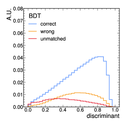
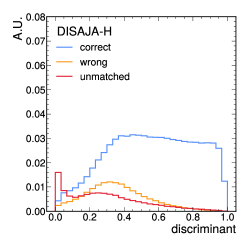
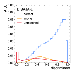
Figure 4: Distribution of the highest $\mathit{{t}{}_{\mspace{-3.0mu}\scriptstyle{}}^{\mspace{-1.0mu}\scriptstyle{}}}\to\mathit{{s}{}_{\mspace{-3.0mu}\scriptstyle{}}^{\mspace{-1.0mu}\scriptstyle{}}}\mathit{{W}{}_{\mspace{-3.0mu}\scriptstyle{}}^{\mspace{-1.0mu}\scriptstyle{}}}$ score used as a discriminant in the signal sample, showing jets that are correctly assigned, wrongly assigned, and unmatched with partons. The ratios for these three categories are reflected in the distributions.

	$\mathit{{t}{}_{\mspace{-3.0mu}\scriptstyle{}}^{\mspace{-1.0mu}\scriptstyle{}}}\to\mathit{{s}{}_{\mspace{-3.0mu}\scriptstyle{}}^{\mspace{-1.0mu}\scriptstyle{}}}\mathit{{W}{}_{\mspace{-3.0mu}\scriptstyle{}}^{\mspace{-1.0mu}\scriptstyle{}}}$	$t\to bW$	other
BDT	76.8%	6.1%	17.0%
DiSaJa-H	82.5%	8.4%	9.1%
DiSaJa-L	86.8%	2.4%	10.9%

Table 3: Ratio of the MC truth matched categories of jet with the highest $\mathit{{t}{}_{\mspace{-3.0mu}\scriptstyle{}}^{\mspace{-1.0mu}\scriptstyle{}}}\to\mathit{{s}{}_{\mspace{-3.0mu}\scriptstyle{}}^{\mspace{-1.0mu}\scriptstyle{}}}\mathit{{W}{}_{\mspace{-3.0mu}\scriptstyle{}}^{\mspace{-1.0mu}\scriptstyle{}}}$ jet score in jet-parton matched $t\bar{t}\to sWbW$ events on each model.

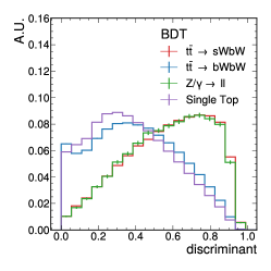
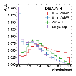
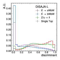
Figure 5: Normalized distributions of the highest $\mathit{{t}{}_{\mspace{-3.0mu}\scriptstyle{}}^{\mspace{-1.0mu}\scriptstyle{}}}\to\mathit{{s}{}_{\mspace{-3.0mu}\scriptstyle{}}^{\mspace{-1.0mu}\scriptstyle{}}}\mathit{{W}{}_{\mspace{-3.0mu}\scriptstyle{}}^{\mspace{-1.0mu}\scriptstyle{}}}$ category scores for jets in events across different classification methods. The left shows the distribution using the BDT. The middle illustrates the distribution using DiSaJa-H, while the right panel displays the distribution using DiSaJa-L. All distributions are normalized to 1 for comparative purposes.

We evaluate the performance of the DiSaJa models by comparing with the BDT model. The highest $\mathit{{t}{}_{\mspace{-3.0mu}\scriptstyle{}}^{\mspace{-1.0mu}\scriptstyle{}}}\to\mathit{{s}{}_{\mspace{-3.0mu}\scriptstyle{}}^{\mspace{-1.0mu}\scriptstyle{}}}\mathit{{W}{}_{\mspace{-3.0mu}\scriptstyle{}}^{\mspace{-1.0mu}\scriptstyle{}}}$ score within each event is used as the discriminant to distinguish between signal and background processes, and the jet with the highest $\mathit{{t}{}_{\mspace{-3.0mu}\scriptstyle{}}^{\mspace{-1.0mu}\scriptstyle{}}}\to\mathit{{s}{}_{\mspace{-3.0mu}\scriptstyle{}}^{\mspace{-1.0mu}\scriptstyle{}}}\mathit{{W}{}_{\mspace{-3.0mu}\scriptstyle{}}^{\mspace{-1.0mu}\scriptstyle{}}}$ score is referred to as the predicted primary $\mathit{{s}{}_{\mspace{-3.0mu}\scriptstyle{}}^{\mspace{-1.0mu}\scriptstyle{}}}$ jet. Fig. 4 shows the distribution of the highest $\mathit{{t}{}_{\mspace{-3.0mu}\scriptstyle{}}^{\mspace{-1.0mu}\scriptstyle{}}}\to\mathit{{s}{}_{\mspace{-3.0mu}\scriptstyle{}}^{\mspace{-1.0mu}\scriptstyle{}}}\mathit{{W}{}_{\mspace{-3.0mu}\scriptstyle{}}^{\mspace{-1.0mu}\scriptstyle{}}}$ score in the signal sample. Events are categorized into three labels: correct (wrong), where a predicted primary $\mathit{{s}{}_{\mspace{-3.0mu}\scriptstyle{}}^{\mspace{-1.0mu}\scriptstyle{}}}$ jet is (is not) the genuine primary $\mathit{{s}{}_{\mspace{-3.0mu}\scriptstyle{}}^{\mspace{-1.0mu}\scriptstyle{}}}$ jet, and unmatched, representing events where the jet-parton matching fails. Table 3 presents the percentages of MC truth categories of predicted primary $\mathit{{s}{}_{\mspace{-3.0mu}\scriptstyle{}}^{\mspace{-1.0mu}\scriptstyle{}}}$ jet. Fig. 5 shows normalized distributions of the score for the signal and background processes using DiSaJa and BDT model. The results demonstrate that the DiSaJa models achieve better assignments to $\mathit{{t}{}_{\mspace{-3.0mu}\scriptstyle{}}^{\mspace{-1.0mu}\scriptstyle{}}}\to\mathit{{s}{}_{\mspace{-3.0mu}\scriptstyle{}}^{\mspace{-1.0mu}\scriptstyle{}}}\mathit{{W}{}_{\mspace{-3.0mu}\scriptstyle{}}^{\mspace{-1.0mu}\scriptstyle{}}}$ than the BDT. Additionally, the DiSaJa-L outperforms the DiSaJa-H.

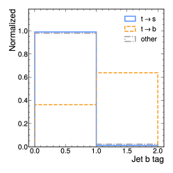
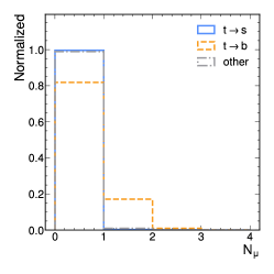
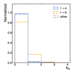
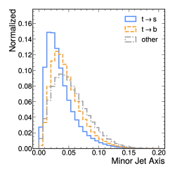
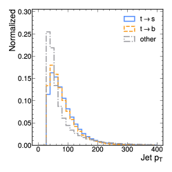
Figure 6: Distributions of high-importance features used in the BDT model training. In all figures, t$\to$q represents q jets from $t\to qW$ decay, and other denotes jets from non-top decays. The figures are arranged in order of feature importance.

To understand the features responsible for the discrimination power, Fig. 6 shows the distributions of high-importance input features for the BDT model. Feature importance is defined as gain, which measures the average improvement in accuracy brought by a feature when used for splitting [49]. The variables with the highest importance are: the value of the $b$ tag, the number of muons in the jet, the number of electrons in the jet, the minor axis, and jet $p_{T}^{.}$ This shows that the BDT model is mainly using $b$-tag-related variables to distinguish the $\mathit{{t}{}_{\mspace{-3.0mu}\scriptstyle{}}^{\mspace{-1.0mu}\scriptstyle{}}}\to\mathit{{s}{}_{\mspace{-3.0mu}\scriptstyle{}}^{\mspace{-1.0mu}\scriptstyle{}}}\mathit{{W}{}_{\mspace{-3.0mu}\scriptstyle{}}^{\mspace{-1.0mu}\scriptstyle{}}}$ jets from $t\to bW$ jets.

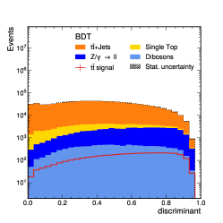
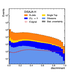
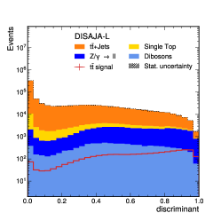
Figure 7: Normalized score distribution for different models at an integrated luminosity of $138$ fb^-1. The BDT model, DiSaJa-H, and DiSaJa-L are compared for signal background separation.

We perform statistical tests to evaluate model performance. For the tests, we use a binned profile likelihood fit using the CMS Combine framework [50]. The observable for the fit is the highest $\mathit{{t}{}_{\mspace{-3.0mu}\scriptstyle{}}^{\mspace{-1.0mu}\scriptstyle{}}}\to\mathit{{s}{}_{\mspace{-3.0mu}\scriptstyle{}}^{\mspace{-1.0mu}\scriptstyle{}}}\mathit{{W}{}_{\mspace{-3.0mu}\scriptstyle{}}^{\mspace{-1.0mu}\scriptstyle{}}}$ assignment score as shown in Fig. 7 and the parameter of interest (POI) is the signal strength $\mu$ scaling the signal yield, defined as $\mu=\frac{|V_{ts}|^{2}}{|V_{ts}^{PDG}|^{2}}$, where $|V_{ts}^{PDG}|=4.110\times 10^{-2}$. Only the statistical uncertainty due to the simulation sample size is considered as a systematic in this study.

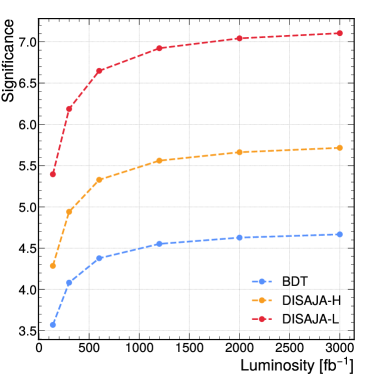
Figure 8: Expected significance of excluding scenarios with $|V_{ts}|=0$, calculated from an integrated luminosity of $138$ fb^-1 to $3000$ fb^-1. The significance is calculated without considering systematic effects.

We calculate the expected significance of excluding $|V_{ts}|=0$ using the test statistic $q=-2\ln\frac{\mathcal{L}(0,\hat{\theta}_{0})}{\mathcal{L}(\hat{\mu},\hat{\theta})}$ where $\mu$ is the signal strength, $\theta$ are the nuisance parameters, and $\hat{\mu}$ and $\hat{\theta}$ are the unconstrained maximum likelihood estimator (MLE) for $\mu$ and $\theta$, respectively, and $\hat{\theta}_{\mu}$ is the value of the nuisance parameters that maximize the likelihood at a given $\mu$. The test statistic is truncated to 0 when $\hat{\mu}<0$. The expected significance is derived using the Asimov dataset and the asymptotic approximation of the profile likelihood ratio [51]. The calculation is performed on the observable distribution normalized to an integrated luminosity of $138$ fb^-1, which is equivalent to the data collected at CMS during the LHC Run 2 period. Then, the expected significance is extrapolated up to $3000$ fb^-1, which is expected to be collected during the upcoming HL-LHC experiment. Fig. 8 illustrates a comparison of the significance for each model. The DiSaJa models outperform the BDT model, and the DiSaJa-L model performs better than the DiSaJa-H model. The DiSaJa-L model shows an expected exclusion significance greater than 5$\sigma$ with the Run 2 luminosity.

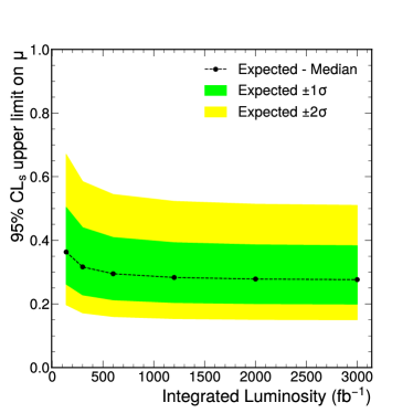
Figure 9: Expected CL_s upper limit on signal strength $\mu$ (DiSaJa-L). The expected CL_s upper limit is calculated from $138$ fb^-1 (CMS Run 2 luminosity) to $3000$ fb^-1 (HL-LHC luminosity) with only luminosity projection without considering the attendant effects.

We calculate the expected CL_s upper limits at the 95% CL using the best-performing model, DiSaJa-L. For the limit calculation, the test statistic $q=-2\ln\frac{\mathcal{L}(\mu,\hat{\theta}_{\mu}))}{\mathcal{L}(\hat{\mu},\hat{\theta}))}$ is employed. Depending on the value of $\hat{\mu}$, the test statistic is modified to $q=-2\ln\frac{\mathcal{L}(\mu,\hat{\theta}_{\mu}))}{\mathcal{L}(0,\hat{\theta_{0}}))}$ for $\hat{\mu}<0$ and is set to $q=0$ for $\hat{\mu}>\mu$ [50]. Using the Asimov dataset with $\mu=0$, the expected median upper limit is derived and the expected $\pm 1\sigma$ and $\pm 2\sigma$ statistical fluctuations are extracted using asymptotic properties of the likelihood function [51], yielding $\mu<0.3633^{+0.1404}_{-0.1012}$ based on the integrated luminosity of Run 2. The upper limit result is also projected to the Run 3 and HL-LHC luminosities and yields $\mu<0.3164^{+0.1236}_{-0.0881}$ and $\mu<0.2764^{+0.1068}_{-0.0770}$, respectively, as shown in Fig. 9.

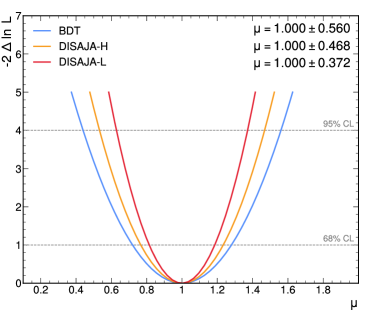
Figure 10: Expected negative log-likelihood scan for the signal strength ($\mu$) on an LHC Run 2 Luminosity ($138$ fb^-1). The DiSaJa-L shows the best performance, providing bounds for $|V_{ts}|$ estimation.

We scan the negative log-likelihood ratio of each model, using the Asimov dataset with $\mu=1$, as a function of the signal strength with the integrated luminosity of Run 2 to obtain the expected confidence interval for the measurement, as shown in Fig. 10. Among the models, DiSaJa-L shows the smallest interval, consistent with the other model comparisons above. With this model, the expected interval is $3.26\times 10^{-2}<|V_{ts}|<4.81\times 10^{-2}$ at the 95% CL.

VI Conclusion

We have studied the application of deep learning for the direct determination of $|V_{ts}|$ in the dileptonic $t\bar{t}$ final state events. The simulated sample reflects the environment of the CMS-like detector at the LHC experiment in the Run 2 period. Taking the primary $\mathit{{s}{}_{\mspace{-3.0mu}\scriptstyle{}}^{\mspace{-1.0mu}\scriptstyle{}}}$ jet tagging approach, we have developed a deep learning-based jet discriminator, which we call DiSaJa-H, which uses as inputs all the high-level reconstructed objects of an event. The performance improvement using the DiSaJa-H method is tested by comparing it to the BDT method, which was used in previous studies, and further performance improvement is achieved by using a model, DiSaJa-L, which uses the jet constituents as input variables. With the DiSaJa-L model, the expected significance for excluding $|V_{ts}|=0$ assuming $|V_{ts}|$ = $|V_{ts}^{PDG}|$ is 5.40$\sigma$, the median expected upper limit on $\mu$ at 95% CL is found to be 0.3633, and the confidence interval is $3.26\times 10^{-2}<|V_{ts}|<4.81\times 10^{-2}$ at the 95% CL. Assuming the same collider environment as the Run 2 used in this paper, the statistical tests are extrapolated by projecting the integrated luminosity to $300$ and $3000$ fb^-1, corresponding to Run 3 and the HL-LHC, respectively. With the Run 3 projection, the results of the Run 2 are improved to 6.19$\sigma$ for the expected significance and $\mu<0.3164$ at the 95% CL is the median expected upper limit. With the HL-LHC projection, they are enhanced to 7.10$\sigma$ and $\mu<0.2764$. The DiSaJa models show a large performance increase over standard machine learning techniques, which will contribute significantly to measurement precision. Furthermore, the flexibility of the multi-domain input and output of the model allows for it to be adapted to other analyses.

References

- Kobayashi and Maskawa [1973] M. Kobayashi and T. Maskawa, CP Violation in the Renormalizable Theory of Weak Interaction, Prog. Theor. Phys. 49, 652 (1973).
- Zyla et al. [2020] P. A. Zyla et al. (Particle Data Group), Review of Particle Physics, PTEP 2020, 083C01 (2020).
- Alwall et al. [2007] J. Alwall, R. Frederix, J. M. Gerard, A. Giammanco, M. Herquet, S. Kalinin, E. Kou, V. Lemaitre, and F. Maltoni, Is V(tb) 1?, Eur. Phys. J. C 49, 791 (2007), arXiv:hep-ph/0607115 .
- Lenz and Nierste [2007] A. Lenz and U. Nierste, Theoretical update of mixing, JHEP 06, 072, arXiv:hep-ph/0612167 .
- King et al. [2019] D. King, A. Lenz, and T. Rauh, Bs mixing observables and —Vtd/Vts— from sum rules, JHEP 05, 034, arXiv:1904.00940 [hep-ph] .
- Aaij et al. [2022] R. Aaij et al. (LHCb), Precise determination of the – oscillation frequency, Nature Phys. 18, 1 (2022), arXiv:2104.04421 [hep-ex] .
- Aoki et al. [2022] Y. Aoki et al. (Flavour Lattice Averaging Group (FLAG)), FLAG Review 2021, Eur. Phys. J. C 82, 869 (2022), arXiv:2111.09849 [hep-lat] .
- Sirunyan et al. [2020a] A. M. Sirunyan et al. (CMS), Measurement of CKM matrix elements in single top quark -channel production in proton-proton collisions at 13 TeV, Phys. Lett. B 808, 135609 (2020a), arXiv:2004.12181 [hep-ex] .
- Ali et al. [2010] A. Ali, F. Barreiro, and T. Lagouri, Prospects of measuring the CKM matrix element at the LHC, Phys. Lett. B 693, 44 (2010), arXiv:1005.4647 [hep-ph] .
- Jang et al. [2022] W. Jang, J. S. H. Lee, I. Park, and I. J. Watson, Measuring directly using strange-quark tagging at the LHC, J. Korean Phys. Soc. 81, 377 (2022), arXiv:2112.01756 [hep-ph] .
- Faroughy et al. [2024] D. A. Faroughy, J. F. Kamenik, M. Szewc, and J. Zupan, Accessing CKM suppressed top decays at the LHC, SciPost Phys. 16, 131 (2024), arXiv:2209.01222 [hep-ph] .
- Lee et al. [2024] J. S. H. Lee, I. Park, I. J. Watson, and S. Yang, Zero-permutation jet-parton assignment using a self-attention network, Journal of the Korean Physical Society 10.1007/s40042-024-01037-3 (2024).
- Pearkes et al. [2017] J. Pearkes, W. Fedorko, A. Lister, and C. Gay, Jet Constituents for Deep Neural Network Based Top Quark Tagging, (2017), arXiv:1704.02124 [hep-ex] .
- Qu et al. [2022] H. Qu, C. Li, and S. Qian, Particle Transformer for Jet Tagging, (2022), arXiv:2202.03772 [hep-ph] .
- ATL [2022] Constituent-Based Top-Quark Tagging with the ATLAS Detector, (2022).
- ATL [2023] Constituent-Based Quark Gluon Tagging using Transformers with the ATLAS detector, (2023).
- Raine et al. [2024] J. A. Raine, M. Leigh, K. Zoch, and T. Golling, Fast and improved neutrino reconstruction in multineutrino final states with conditional normalizing flows, Physical Review D 109, 012005 (2024).
- Qiu et al. [2023] S. Qiu, S. Han, X. Ju, B. Nachman, and H. Wang, Holistic approach to predicting top quark kinematic properties with the covariant particle transformer, Physical Review D 107, 114029 (2023).
- Zurbano Fernandez et al. [2020] I. Zurbano Fernandez et al., High-Luminosity Large Hadron Collider (HL-LHC): Technical design report, CERN Yellow Reports 10/2020, 10.23731/CYRM-2020-0010 (2020).
- Agarwal [2001] A. G. Agarwal, Proceedings of the Fifth Low Temperature Conference, Madison, WI, 1999, Semiconductors 66, 1238 (2001).
- Ball et al. [2017] R. D. Ball et al. (NNPDF), Parton distributions from high-precision collider data, Eur. Phys. J. C 77, 663 (2017), arXiv:1706.00428 [hep-ph] .
- Czakon and Mitov [2014] M. Czakon and A. Mitov, Top++: A Program for the Calculation of the Top-Pair Cross-Section at Hadron Colliders, Comput. Phys. Commun. 185, 2930 (2014), arXiv:1112.5675 [hep-ph] .
- Sjöstrand et al. [2015] T. Sjöstrand, S. Ask, J. R. Christiansen, R. Corke, N. Desai, P. Ilten, S. Mrenna, S. Prestel, C. O. Rasmussen, and P. Z. Skands, An introduction to pythia 8.2, Computer Physics Communications 191, 159–177 (2015).
- Gehrmann et al. [2014] T. Gehrmann, M. Grazzini, S. Kallweit, P. Maierhöfer, A. von Manteuffel, S. Pozzorini, D. Rathlev, and L. Tancredi, Production at Hadron Colliders in Next to Next to Leading Order QCD, Phys. Rev. Lett. 113, 212001 (2014), arXiv:1408.5243 [hep-ph] .
- Grazzini et al. [2016] M. Grazzini, S. Kallweit, D. Rathlev, and M. Wiesemann, production at hadron colliders in NNLO QCD, Phys. Lett. B 761, 179 (2016), arXiv:1604.08576 [hep-ph] .
- Cascioli et al. [2014] F. Cascioli, T. Gehrmann, M. Grazzini, S. Kallweit, P. Maierhöfer, A. von Manteuffel, S. Pozzorini, D. Rathlev, L. Tancredi, and E. Weihs, ZZ production at hadron colliders in NNLO QCD, Phys. Lett. B 735, 311 (2014), arXiv:1405.2219 [hep-ph] .
- Frederix and Frixione [2012] R. Frederix and S. Frixione, Merging meets matching in MC@NLO, JHEP 12, 061, arXiv:1209.6215 [hep-ph] .
- Sirunyan et al. [2020b] A. M. Sirunyan et al. (CMS), Extraction and validation of a new set of CMS PYTHIA8 tunes from underlying-event measurements, Eur. Phys. J. C 80, 4 (2020b), arXiv:1903.12179 [hep-ex] .
- de Favereau et al. [2014] J. de Favereau, C. Delaere, P. Demin, A. Giammanco, V. Lemaître, A. Mertens, and M. Selvaggi, Delphes 3: a modular framework for fast simulation of a generic collider experiment, Journal of High Energy Physics 2014, 10.1007/jhep02(2014)057 (2014).
- Cacciari et al. [2012] M. Cacciari, G. P. Salam, and G. Soyez, Fastjet user manual, The European Physical Journal C 72, 10.1140/epjc/s10052-012-1896-2 (2012).
- CMS [2016] Identification of b quark jets at the CMS Experiment in the LHC Run 2, Tech. Rep. CMS-PAS-BTV-15-001 (CERN, Geneva, 2016).
- Sirunyan et al. [2018] A. M. Sirunyan et al. (CMS), Identification of heavy-flavour jets with the CMS detector in pp collisions at 13 TeV, JINST 13 (05), P05011, arXiv:1712.07158 [physics.ins-det] .
- Chatrchyan et al. [2014] S. Chatrchyan et al. (CMS), Description and performance of track and primary-vertex reconstruction with the CMS tracker, JINST 9 (10), P10009, arXiv:1405.6569 [physics.ins-det] .
- Sirunyan et al. [2019a] A. M. Sirunyan, A. Tumasyan, W. Adam, F. Ambrogi, E. Asilar, T. Bergauer, J. Brandstetter, M. Dragicevic, J. Erö, and et al., Measurements of differential cross sections in proton-proton collisions at tev using events containing two leptons, Journal of High Energy Physics 2019, 10.1007/jhep02(2019)149 (2019a).
- Sirunyan et al. [2019b] A. M. Sirunyan et al. (CMS), Measurement of the production cross section, the top quark mass, and the strong coupling constant using dilepton events in pp collisions at 13 TeV, Eur. Phys. J. C 79, 368 (2019b), arXiv:1812.10505 [hep-ex] .
- Tumasyan et al. [2023] A. Tumasyan et al. (CMS), Measurement of the top quark pole mass using +jet events in the dilepton final state in proton-proton collisions at = 13 TeV, JHEP 07, 077, arXiv:2207.02270 [hep-ex] .
- Sirunyan et al. [2021] A. M. Sirunyan et al. (CMS), Electron and photon reconstruction and identification with the CMS experiment at the CERN LHC, JINST 16 (05), P05014, arXiv:2012.06888 [hep-ex] .
- Vaswani et al. [2017] A. Vaswani, N. Shazeer, N. Parmar, J. Uszkoreit, L. Jones, A. N. Gomez, L. u. Kaiser, and I. Polosukhin, Attention is all you need, in Advances in Neural Information Processing Systems, Vol. 30, edited by I. Guyon, U. V. Luxburg, S. Bengio, H. Wallach, R. Fergus, S. Vishwanathan, and R. Garnett (Curran Associates, Inc., 2017).
- Hendrycks and Gimpel [2016] D. Hendrycks and K. Gimpel, Gaussian error linear units (gelus), arXiv preprint arXiv:1606.08415 (2016).
- Srivastava et al. [2014] N. Srivastava, G. Hinton, A. Krizhevsky, I. Sutskever, and R. Salakhutdinov, Dropout: A simple way to prevent neural networks from overfitting, Journal of Machine Learning Research 15, 1929 (2014).
- CMS [2013] Performance of quark/gluon discrimination in 8 TeV pp data, Tech. Rep. (CERN, Geneva, 2013).
- Cornelis [2014] T. Cornelis (CMS), Quark-gluon Jet Discrimination At CMS, in 2nd Large Hadron Collider Physics Conference (2014) arXiv:1409.3072 [hep-ex] .
- Field and Feynman [1978] R. D. Field and R. P. Feynman, A Parametrization of the Properties of Quark Jets, Nucl. Phys. B 136, 1 (1978).
- Krohn et al. [2013] D. Krohn, M. D. Schwartz, T. Lin, and W. J. Waalewijn, Jet Charge at the LHC, Phys. Rev. Lett. 110, 212001 (2013), arXiv:1209.2421 [hep-ph] .
- Waalewijn [2012] W. J. Waalewijn, Calculating the Charge of a Jet, Phys. Rev. D 86, 094030 (2012), arXiv:1209.3019 [hep-ph] .
- Loshchilov and Hutter [2017] I. Loshchilov and F. Hutter, Decoupled weight decay regularization, arXiv preprint arXiv:1711.05101 (2017).
- Watanabe [2023] S. Watanabe, Tree-structured parzen estimator: Understanding its algorithm components and their roles for better empirical performance, arXiv preprint arXiv:2304.11127 (2023).
- Akiba et al. [2019] T. Akiba, S. Sano, T. Yanase, T. Ohta, and M. Koyama, Optuna: A next-generation hyperparameter optimization framework (2019), arXiv:1907.10902 [cs.LG] .
- Chen and Guestrin [2016] T. Chen and C. Guestrin, Xgboost: A scalable tree boosting system, in Proceedings of the 22nd acm sigkdd international conference on knowledge discovery and data mining (2016) pp. 785–794.
- Hayrapetyan et al. [2024] A. Hayrapetyan et al. (CMS), The CMS Statistical Analysis and Combination Tool: COMBINE, (2024), arXiv:2404.06614 [physics.data-an] .
- Cowan et al. [2011] G. Cowan, K. Cranmer, E. Gross, and O. Vitells, Asymptotic formulae for likelihood-based tests of new physics, Eur. Phys. J. C 71, 1554 (2011), [Erratum: Eur.Phys.J.C 73, 2501 (2013)], arXiv:1007.1727 [physics.data-an] .