Bayesian Power and Sample Size Calculations for Bayes Factors in the Binomial Setting
Abstract
Bayesian design of experiments and sample size calculations usually rely on complex Monte Carlo simulations in practice. Obtaining bounds on Bayesian notions of the false-positive rate and power therefore often lack closed-form or approximate numerical solutions. In this paper, we focus on the sample size calculation in the binomial setting via Bayes factors, the predictive updating factor from prior to posterior odds. We discuss the drawbacks of sample size calculations via Monte Carlo simulations and propose a numerical root-finding approach which allows to determine the necessary sample size to obtain prespecified bounds of Bayesian power and type-I-error rate almost instantaneously. Real-world examples and applications in clinical trials illustrate the advantage of the proposed method. We focus on point-null versus composite and directional hypothesis tests, derive the corresponding Bayes factors, and discuss relevant aspects to consider when pursuing Bayesian design of experiments with the introduced approach. In summary, our approach allows for a Bayes-frequentist compromise by providing a Bayesian analogue to a frequentist power analysis for the Bayes factor in binomial settings. A case study from a Phase II trial illustrates the utility of our approach. The methods are implemented in our R package bfpwr.
Keywords: Bayesian hypothesis testing; design prior; Bayesian statistics; phase II clinical trial; Monte Carlo simulation
1 Introduction
To ensure efficient and ethical use of resources, sample size calculations are an essential component of experimental design in both frequentist and Bayesian statistics. Accurate planning of the sample size is particularly important in the context of hypothesis testing. There, a prespecified power under the alternative hypothesis is desired and the probability of incorrectly rejecting the null hypothesis needs to be bounded, which often resembles the conventional -level of (Bijma et al., 2017), or when a one-sided test is used (Matthews, 2006). While there exist a plethora of formulas for sample size calculation for standard frequentist tests such as the test or chi-squared test (Matthews, 2006), the situation is not this simple for Bayesian statisticians.
Bayesian statistics is first and foremost troubled by the existence of various indices for hypothesis testing (Kelter, 2021c). For example, one might decide to use posterior probabilities and given the data to test versus . Alternatively, one could opt for the Bayes factor , the predictive updating factor from prior to posterior odds:
| (1) |
Sample size planning and the resulting power under can (and often does) vary for different approaches to testing, such as posterior probabilities and Bayes factors (Kelter, 2020b).
However, the more pressing problem with Bayesian sample size calculations is that in contrast to frequentist hypothesis testing, there exist little to no closed-form or at least numerical solutions. The question how large a sample size should be to provide a power of e.g. , and a type-I-error rate of e.g. , must therefore often rely on simulation (compare Section 1.1). Although power and type-I-error rates are no original Bayesian concepts per se, the idea to compute frequentist metrics of Bayesian indices for hypothesis testing is widely present in the literature (Pourmohamad and Wang, 2023; Grieve, 2022; Rosner, 2021; Kleijn, 2022; Weiss, 1997; Santis, 2004) and ranges back to Good (1983, 1960) and Kerridge (1963). Further perspectives on such Bayes-frequentist compromises in the sense of “frequentistically calibrated” Bayesian approaches are given by Dawid (1982), Rubin (1984), Little (2006) and Grieve (2016). The calibrated Bayes approach is often also recommended by health authorities, for example, the U.S. Food and Drug Administration accepts Bayesian analysis if they are appropriately calibrated in a frequentist sense (U.S. Food and Drug Administration, 2010).
Such a hybrid perspective on Bayesian design of experiments takes the stance to investigate the long-term behaviour of Bayesian quantities like posterior probabilities or Bayes factors, to compute Bayesian versions of power and type-I-error such as
| (2) |
For example, for – the usual threshold for strong evidence according to the scale of Jeffreys (1939) – when holds, the probability to obtain a Bayes factor indicating strong evidence against the null hypothesis (that is, in favour of the alternative ) is bounded by under .111This holds because and amounts to the Bayes factor in favour of indicating (at least) strong evidence for . Thus, resembles an intuitive Bayesian type-I-error rate. Thus, for the Bayesian type-I-error rate is controlled at then. Likewise, if for, say and , the probability to obtain strong evidence in favour of , when is true, is .222This holds because . A critical goal in Bayesian design of experiments and sample size calculation therefore is to provide solutions to the inequalities
| (3) |
for some and in . We close the introduction with two comments.
-
We decided to use thresholds in the conditions Equation 3 because this is the original Bayes factor orientation of Jeffreys (1939) who also used instead of . Therefore, we opt for using the Bayes factor in favour of in all our conditions and formulations, in particular, in the notation of a Bayesian type-I-error rate and Bayesian power as shown in Equation 3. However, if desired, all equations and results can be easily converted to the orientation by taking the reciprocal of the Bayes factor and and inverting inequalities.
-
A further advantage of this notation is that small values of indicate evidence against the null hypothesis , which is in line with frequentist reasoning when using p-values. Accommodating our approach should therefore cause no trouble for frequentists who want to use a Bayesian design with desirable frequentist properties. Note that the latter property does not hold for , where small values indicate evidence in favour of the null hypothesis .
1.1 The curse of the Monte Carlo standard error
As noted above, there are little to no closed-form formulas or at least numerical solutions in almost all practically relevant settings, which allow to compute Equation 2 in a simple manner with some notable exceptions such as and test Bayes factors (Weiss, 1997; Santis, 2004; Pawel and Held, 2024; Wong and Tendeiro, 2024). Thus, the status quo in Bayesian design of experiments and sample size planning often relies on simulation, and the usual standard consists of conducting a Monte Carlo simulation to investigate the quantities in Equation 2 (Schönbrodt et al., 2017; Schönbrodt and Wagenmakers, 2018; Stefan et al., 2022; Grieve, 2022; Kelter, 2020b, 2021a, 2021d, 2021b; Makowski et al., 2019; Kelter and Schnurr, 2024; D. A. Berry, 2006; S. M. Berry, 2011; Wang and Gelfand, 2002). In this section, we outline a principal problem connected with this approach.
Monte Carlo simulations are abundant in Bayesian sample size calculation in the context of hypothesis testing (S. M. Berry, 2011; Grieve, 2022; Schönbrodt et al., 2017). They typically proceed as follows: First, simulation of a parameter value , under or is necessary. Then, for each parameter value , a data set of size needs to be simulated, so there are data sets of sample size . Subsequently, the computation of the quantity of interest (e.g. the Bayes factor) based on these realizations follows. Due to the strong law of large numbers, the Monte Carlo average then converges for against the desired probability (Robert and Casella, 2004), for example:
| (4) |
where we suppose that the parameter draws are simulated according to in Equation 4. Here, denotes the indicator function, which takes value if and else . This Monte Carlo estimate provides an estimate for the fixed sample size based on simulated data sets. In practice, the threshold and sample size need to be balanced to fulfill Equation 3. However, a reliable bound on the Bayesian type-I-error (and likewise, Bayesian power) is obtained only, if is large enough.
A problem now occurs as Monte Carlo uncertainty enters the stage. As noted in Morris et al. (2019), Monte Carlo standard errors are essential to quantify the uncertainty of a Monte Carlo estimate due to the finiteness of the simulation size . For example, using simulated realizations of the data of sample size under will produce a less reliable estimate of than using simulated realizations. Providing a Monte Carlo standard error is therefore quintessential to indicate the uncertainty due to simulation, a proposal that was also included in the Bayesian Simulation Study (BASIS) framework of Kelter (2023). However, guidelines and tutorials in Bayesian Monte Carlo simulation (e.g. Kruschke, 2021; Depaoli and van de Schoot, 2017; Van de Schoot et al., 2021; Schönbrodt et al., 2017; Stefan et al., 2019) often recommend fixed values such as . This is clearly inadequate, as in one case may be enough, while in another it may result in an unacceptably large Monte Carlo standard error. Even when may be enough, it could be “too much” in the sense that would produce a sufficiently small Monte Carlo standard error and the computational resources could have been used more effectively otherwise.
Taking stock, Monte Carlo simulations provide a working but computationally expensive tool for Bayesian design of experiments and sample size calculations. The Monte Carlo uncertainty inherent to these approaches troubles Bayesian sample size calculations as it often undermines the reliability of a simulation-based result when not taken carefully into account.333We emphasize that Monte Carlo simulations are of course helpful and necessary when no other solutions are available, but simultaneously stress that Monte Carlo standard errors must then accompany the Monte Carlo estimate. We omit details on the computational approaches to compute a Monte Carlo standard error (which include Bootstrap resampling, see the appendix in Kelter (2023)) and only note that they usually add another layer of complexity and computational effort to the possibly already demanding simulation study. Currently, there is a lack of other approaches such as closed-form solutions or numerical approximations to solve Equation 3. We now turn to our solution to this problem and provide an outline of what this paper contributes to the existing literature.
1.2 Outline
In this paper, we propose a sample size calculation procedure for Bayes factors in the binomial setting outlined in the next section and already discussed briefly in Section 1. Figure 1 provides an overview about the approach, and while the idea is generalizable to other settings such as tests, tests (Pawel and Held, 2024; Wong and Tendeiro, 2024) and other situations, we restrict the focus of the current manuscript to the binomial setting. The latter is important in phase II clinical trials with binary endpoint, where the proof of concept of a novel drug is studied. Other applications are given in Section 3.
The plan of the paper is as follows: Section 2 outlines the main idea and key steps depicted in Figure 1. We detail the two most relevant hypothesis tests in the binomial model, that is, the point-null versus composite test versus and the directional test of versus . We obtain the one-sided test of versus as a special case under our chosen priors. Therefore, we detail the derivation of the Bayes factor and walk through the entire process depicted in Figure 1. We illustrate the idea in Section 3 and provide real world examples. The ultimate goal as shown in Figure 1 is to obtain a calibrated Bayesian experimental design in the sense that one or both inequalities in Equation 3 are fulfilled. In the following section Section 4 we also discuss alternatives to this frequentist approach in the sense that other metrics could be of interest to a Bayesian, such as the probability to confirm when it is indeed true. We close in Section 5 with a discussion and outlook for future research.

2 The root-finding approach to Bayesian sample size calculation
2.1 One-sided hypothesis test
Our main assumption here is that the observed data random variable follows a binomial distribution with parameters and , . Its probability mass function is given as
| (5) |
for . In this setting, we have , so the parameter space is the unit interval. First, a prior is chosen for the parameter . The distribution is a conjugate prior for the binomial likelihood, and when chosen as the prior, the posterior is also Beta-distributed (Held and Sabanés Bové, 2014):
As a consequence, a natural choice for a prior is the beta distribution. We first deal with the one-sided hypothesis test of
| (6) |
for some . This situation arises for example in single-arm clinical phase II studies which aim at demonstrating the efficacy of a potential novel drug or therapy (H. Zhou et al., 2017; Kelter and Schnurr, 2024).
2.1.1 Choice of the design and analysis prior
The first step for the sample size calculation approach is shown as steps 1 and 2 in Figure 1. Thus, a so called design prior and analysis prior must be chosen (O’Hagan and Stevens, 2001). We denote the former by and the latter by . The idea of the design prior is that we base the planning of the sample size and properties such as the Bayesian type-I-error rate and power – compare Equation 2 – on this prior . However, the planning stage might include subjective beliefs, so the analysis – in this case a Bayes factor test – should be based on another (more objective) prior distribution .444These objective beliefs could result in a design that does not meet our demands formulated in Equation 3. When choosing , the design and analysis prior agree and we base both the planning and analysis of the study on the same distribution.
Therefore, we start with the design prior and must choose a prior under and under , to use the prior-predictive density in a second step to calculate our desired quantities in Equation 3. Therefore, we choose truncated Beta priors both under and as follows:
| (7) |
where denotes the truncated Beta distribution to the interval with density
| (8) |
where denotes the regularized incomplete beta function, defined as , is the incomplete beta function, and is the Beta function. The last equality in Equation 8 follows from . The regularized incomplete beta function is the cumulative distribution function of the beta distribution. In brief terms, the truncated Beta distribution on simply normalizes the untruncated Beta distribution on to the interval of .
Likewise, we pick the truncated Beta distribution under , this time normalized to :
| (9) |
For the analysis prior under and , we also choose truncated Beta priors, with possibly different values and , where the subscript signals that the hyperparameters belong to our analysis instead of design prior:
| (10) | |||
| (11) |
These priors allow for huge flexibility in incorporating both subjective and objective beliefs about under respectively . For example, a uniform prior is obtained when respectively , and other values of the hyperparameters can indicate strong a priori beliefs about the truth of certain parameter regions in (Kruschke, 2014), see Figure 2 for an illustration. Also, the Beta distribution has the property that for large
| (12) |
More precisely, if , then converges in distribution to as increases. Therefore, choosing and letting with large enough therefore amounts to using a highly informative prior which converges against a Dirac measure on , and which equals a frequentist power calculation in the sense that the Bayesian prior calculates power (or the Bayesian type-I-error rate) under the point-value . Importantly, using such a prior reduces to the point-null hypothesis , and therefore the directional test of against reduces to the one-sided test of against .

2.1.2 Derivation of the prior-predictive distribution
The third step shown in Figure 1 consists of deriving the prior-predictive probability mass function and under the null and alternative hypothesis. These probability mass functions will be used together with the Bayes factor later, to compute critical values , for which we can state that passes a given threshold such as . Based on the predictive distributions we can then compute the desired probabilities and , compare Equation 3. Achieving a specified power will then proceed by selecting the smallest sample size for which the predictive probability
for a specified such as , where denotes the predictive distribution under .
Based on the standard Beta prior, marginalizing out of the binomial likelihood yields the posterior predictive distribution which is Beta-Binomial
| (13) |
where successes have been observed out of samples. However, here we base the predictive probability mass function on the truncated beta design priors under and to obtain a prior-predictive distribution. This leads to the following predictive probability mass function of the data based on a fixed and a truncated beta prior for with , for details see the Appendix:
| (14) |
Conditioning on then leads to , where in the above, we can replace by and by . For , we obtain where we replace by and by . Depending on which design prior we use, we further replace and by the selected values and in the design prior under in Equation 7, respectively in the design prior under in Equation 9. We stress that the predictive distribution in Equation 14 makes use of the design priors chosen in advance.
2.1.3 Derivation of the Bayes factor
The next step is step 4 in Figure 1, the derivation of the Bayes factor. Therefore, we must choose analysis priors under and . We opt for the same truncated beta priors here, stressing that it is well possible to choose different hyperparameters and in the analysis than in the design prior (where the hyperparameters were and ). It is, of course, possible to choose design and analysis prior identically.
For versus with truncated Beta priors and we arrive at the Bayes factor
| (15) |
where a derivation is provided in the Appendix.
2.1.4 Numerical root-finding
Based on the Bayes factor, the fifth step in Figure 1 now consists of numerical root-finding. In brief terms, the idea is to find a solution to the equation
| (16) |
by numerical means for a fixed sample size . Thus, we use Equation 15 and numerically find the root of via Newton’s method as, for example, implemented in the uniroot function in the statistical programming language R (Team, 2020).
2.1.5 Computation of critical value(s)
The solution of Equation 16 yields a value based on which we can state that for we have (e.g. ), that is, evidence for the alternative – as measured by – is at least . Note that the analysis prior is used to compute the Bayes factor.
2.1.6 Computation of Bayesian type-I-error rate and power
Based on the root found in the last step, the seventh step in Figure 1 consists of computing the relevant quantities and where we have
and
and the former is equal to the Bayesian type-I-error rate, while the latter is the Bayesian analogue to frequentist power, compare Equation 3.
2.1.7 Sample size calculation for the Bayes factor
The ultimate goal now is to obtain the sample size for which we can state that exceeds a given threshold, such as for , so we have at least Bayesian power to find at least evidence for . It might happen that for a fixed there is no so that the threshold is fulfilled. Then, increasing will eventually lead to the situation where a large (or small) enough Bayes factor can be found. This is due to the fact that for a large enough sample size there must be a number of successes for which holds due to the asymptotic properties of the Bayes factor (Kleijn, 2022).
2.2 Two-sided hypothesis test
Now, the second option is to use a two-sided hypothesis test of versus .
2.2.1 Design and analysis priors
Based on the same assumption , a Dirac measure in is chosen as the analysis prior under , that is,
where as under , a Beta prior is selected:
with hyperparameters .
The design priors are chosen as follows: Under , the lower truncation point is , and the upper truncation point . The design prior under therefore becomes a normal Beta prior with hyperparameters . Under , a Dirac measure is chosen in again.
2.2.2 Derivation of the prior-predictive
From Equation 14 we obtain now the prior-predictive distribution by setting and under . Under , the prior-predictive probability mass function reduces to
Under , we can use the design prior given in Equation 14 with and and appropriate hyperparameters and plugged in for and .
2.2.3 Derivation of the Bayes factor
For the point null test of versus with prior , the Bayes factor results in
| (17) |
where a derivation is provided in the Appendix.
3 Examples
3.1 Single-arm phase II proof of concept trial with binary endpoint
In this subsection, we adopt an example of a clinical trial discussed in Kelter and Schnurr (2024) in the context of sequential design. There, a single-arm phase IIA study to demonstrate the efficacy of a novel drug or therapy is considered and the primary endpoint is binary. The primary objective of the study was to assess the efficacy of a combination therapy as front-line treatment in patients with advanced nonsmall cell lung cancer. The study involved the combination of a vascular endothelial growth factor antibody plus an epidermal growth factor receptor tyrosine kinase inhibitor. The primary endpoint is the clinical response rate, that is, the rate of complete response and partial response combined, to the new treatment. The hypotheses of interest are given as
The current standard treatment yields a response rate of 20% , so we have . The target response rate of the new regimen is 40%, so . We stress that somewhat unrealistic, the parameter interval is somehow excluded from the hypotheses considered, a choice that is sometimes seen in phase IIA studies, compare Lee and Liu (2008). While such a distance between and allows for an easier separation between both hypotheses via statistical testing, we refrain from doing so and instead select a flat prior with to stay neutral first. Later, we also opt for the more realistic choice to center a truncated Beta design prior on , so we select for the mode of the design prior, details follow below. Under , we select a flat Beta design prior, and we formally test
here. For the analysis priors, we also select flat truncated Beta priors both under and , that is, in Equation 10 and Equation 11. This choice of design and analysis priors intuitively seems objective.
In Kelter and Schnurr (2024), a sequential design was used and calibrated via a Monte Carlo simulation to attain the boundaries and for the Bayesian type-I-error rate and power. This choice is widely adopted in phase II trials (Lee and Liu, 2008; H. Zhou et al., 2017; S. M. Berry, 2011), so we opt for these boundaries in the context of our Bayesian design requirements given in Equation 3. However, we do not use a sequential but fixed sample size design, which allows for much easier conduct of the trial, possibly at the cost of a less efficient design. Still, sequential designs are logistically much more challenging, and additionally troubled by the need to calibrate a Monte Carlo simulation and attain sufficiently small Monte Carlo standard errors (T. Zhou and Ji, 2023). Thus, we need to calculate a sample size so that
where we select the threshold for strong evidence.
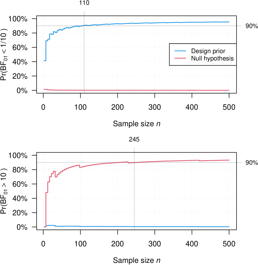
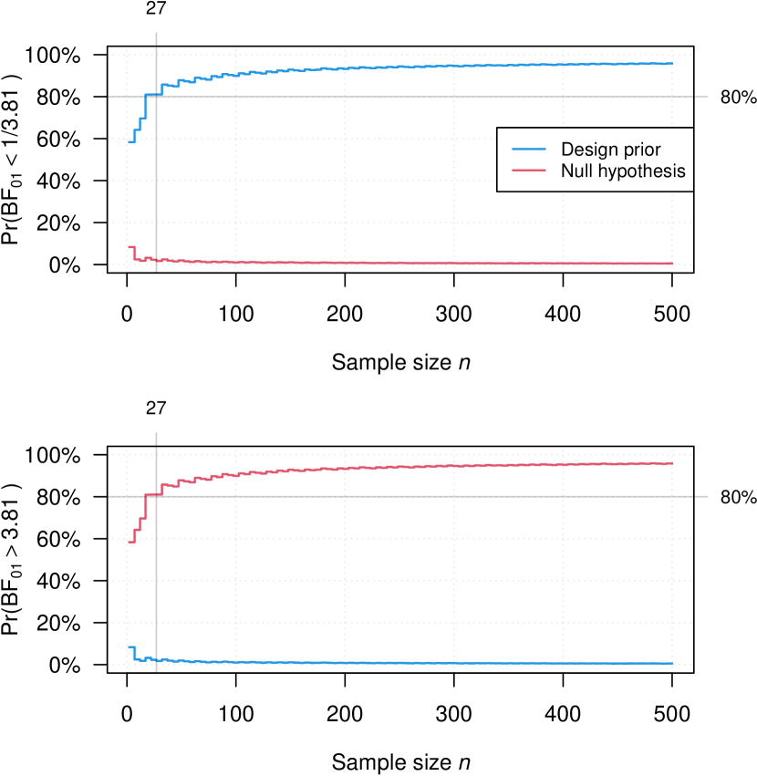
Application of the root-finding approach shown in Figure 1 then yields a sample size of . This sample size leads to a power of (under ) under the truncated design beta design prior , while under the null (i.e., a uniform prior from 0 to 0.2) the Bayesian type-I-error rate is . The top plot in Figure 3(a) shows the corresponding Bayesian power and type-I-error curves.555In the binomial model, it happens that power and type I error viewed as a function of the sample size show “oscillation” or “zig-zag” behaviours as visible in Figure 3-8(b). That is, due to the discreteness of the data, it can happen that the power (type I error rate) increases (decreases) but then decreases (increases) again when the sample size is increased. These behaviours are not limited to Bayes factors but occur for many other methods in the binomial model, see e.g. chapter 17 in Julious (2023) for illustration of oscillating power of binomial tests, or section 2 in Brown et al. (2001) for oscillating coverage rates of confidence intervals for a binomial proportion. For this reason, it is important to verify that a calculated sample size truly ensures a power (type I error rate) above (below) the target power (type I error rate) for any greater sample size. In the bfpwr package this is implemented via an algorithm that terminates the numerical search only if power (type I error) does not drop below (increase above) the target for at least 10 additional observations, otherwise the numerical search is continued. The blue solid line is the Bayesian power, while the red solid line is the associated Bayesian type-I-error rate, compare Equation 3.
Finally, the type-I-error rate and power related to under the point values and are given by and , respectively. Hence, the design is calibrated also from a fully frequentist perspective – which uses Bayes factors as test statistics, a concept originally proposed by Good (1983).
Now, the bottom plot in Figure 3(a) additionally shows the probability to obtain compelling evidence in form of a Bayes factor larger than in favour of the null hypothesis . This probability can be denoted as the Bayesian power to obtain compelling evidence for . Thus, for patients, we have at least 90% power to accept based on strong evidence with . Note that such a perspective on Bayesian power is not available in frequentist testing, and also not formally required according to Equation 3. However, in practice, stopping a phase II a trial when a drug is inefficient is highly desirable (S. M. Berry, 2011; Lee and Liu, 2008; H. Zhou et al., 2017; Kelter and Schnurr, 2024). One reason is that due to the possibly large number of potentially effective agents, filtering promising ones from ineffective drugs is important. This is one primary reason to consider sequential designs after all, as they allow early stopping for futility, see for example H. Zhou et al. (2017) and Kelter and Schnurr (2024). In the calibrated design shown in Figure 3(a), we can be quite certain – with at least probability – that we will stop for futility based on patients.
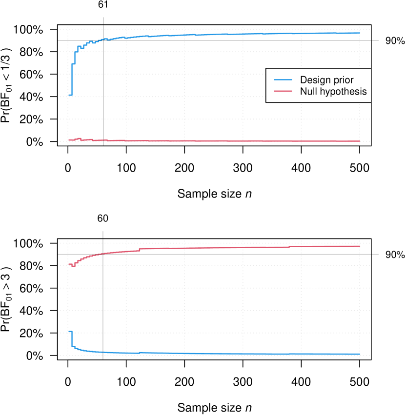
The sample sizes and seem prohibitively large for a phase II trial. Thus, Figure 3(b) demonstrates the effect of using the same design and analysis priors with a more liberal threshold , which amounts to only moderate evidence (Jeffreys, 1939). This is an assumption which is readily justified in the context of a single-arm phase II trial. As shown in the upper plot of Figure 3(b), now patients suffice to achieve at least 90% Bayesian power, and the probability to obtain compelling evidence in favour of – as shown in the bottom plot of Figure 3(b) – reaches 90% already after patients. We see that based on the more realistic threshold in a phase II trial, the sample sizes required for carrying out such a study become realistic.
The advantage of the two sample size calculations above are their realism: The truncated design priors include also parameter values very close to the boundary between and , and thus the calculated sample sizes become large because separation between and becomes naturally more difficult. The advantage of the realism is the price paid in sample size required, and a practically possible solution to this aspect is to consider the frequentist limit as described in Equation 12.
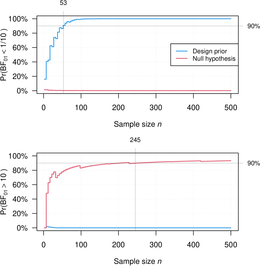
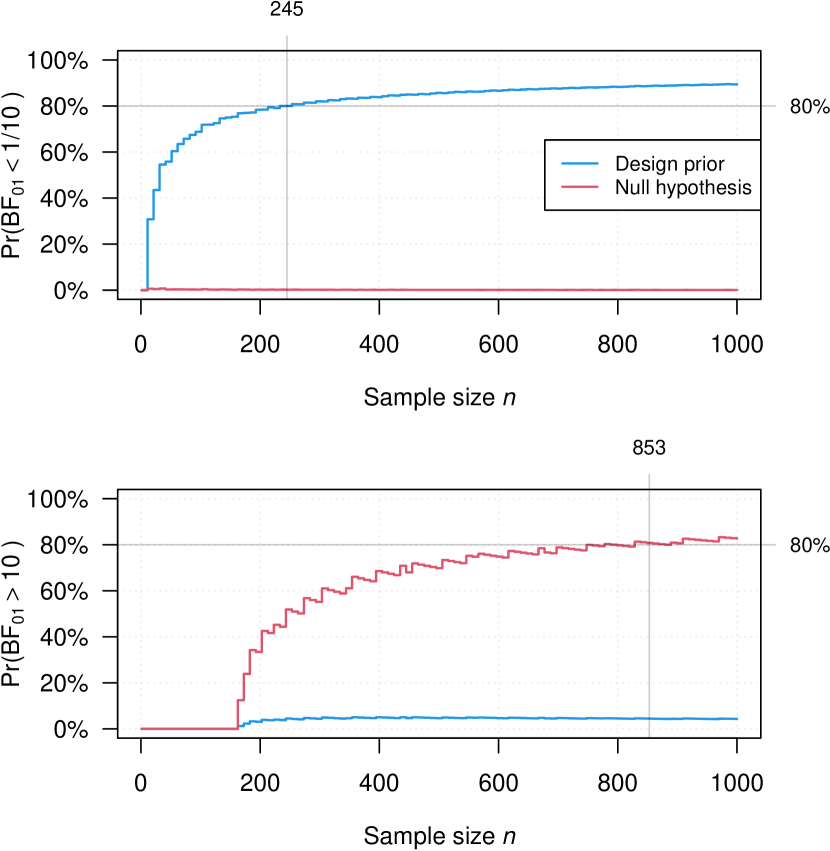
Thus, we reduce the truncated Beta design prior to a point-prior in next. Sample sizes under are thus calculated based on a single parameter value without taking into account its uncertainty. Sample size calculation under proceeds as before in Figure 3(b). The bottom part of Figure 4(b) therefore yields identical results like the one in Figure 3(a), and after patients we can state with at least 90% probability that the drug is ineffective if holds. The top part in Figure 4(b) now shows that under the point-prior with all probability mass on we arrive at patients required to yield a calibrated Bayesian design based on the Bayes factor. Note that under – see the bottom plot in Figure 4(b) – nothing changes, because the Bayesian power to find compelling evidence for the null is still averaged under the truncated Beta prior on , that is, .
In sum, shifting the evidence threshold to yields achievable and realistic sample sizes in terms of calibrating Bayesian power and type-I-error rate, as shown above. Additionally, the sample sizes required to calibrate the probability to find compelling evidence for the null hypothesis are also practically attainable.
However, by now all sample size calculations were based on a flat design prior with under , compare Equation 9, and with under , compare Equation 7. A different choice is given by using a design prior that is centered at some , so under we have the expectation that the drug is effective in some way.666Importantly, we must not necessarily believe a priori that such an effectiveness is most probable without any observed data. We can also just interpret such a centered prior as the design prior which expresses the sample size requirements for a minimally relevant effect size of interest. If, e.g. we center the prior at , we can argue that the resulting sample sizes based on the root-finding approach are most realistic if the true effect size is somewhere around . If the drug is more effective, the calculated sample sizes will be too large. If the drug is less effective, they will be too small. The latter two aspects depend in turn on how strongly centered the design prior is around .Therefore, we consider three scenarios: First, we could center the mean of the Beta distribution at . Second, we could center the mode of the Beta distribution at . Third, we could center both at . As shown in the Appendix, the third option is possible only if , which is not helpful. Therefore, we need to decide between mean- and mode-centering at some . We pick mode-centering, primarily because this aligns with the notion of a frequentist power analysis where we are interested in a specific point under the alternative hypothesis . Thus, mode-centering allows to specify which is the most probable point under according to our assumptions in the design stage.
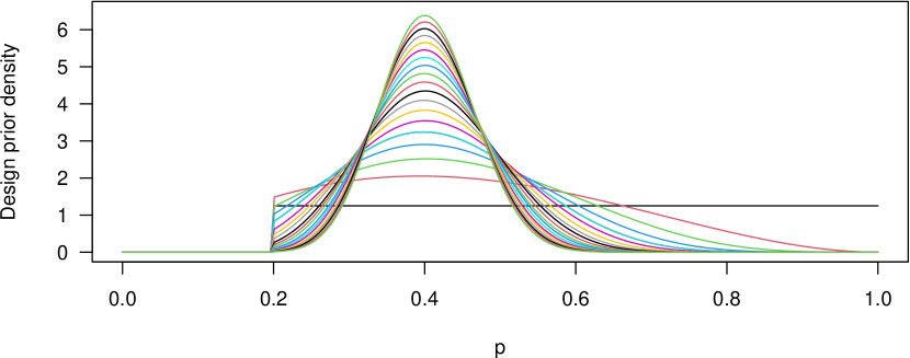
Figure 5 shows several truncated design priors centered at the mode for increasingly informative hyperparameters and . As the mode of the truncated Beta distribution is given as , it is possible to obtain from for some that
| (18) |
for details see the Appendix. Therefore, for each chosen value of , selecting as in Equation 18 yields a truncated Beta design prior centered at . For , one obtains the values shown in Table 1. The parameters at the top are less informative, and the parameters at the bottom are the most informative. This can also be interpreted as follows: For example, and implies that the informativity of our prior equals the information which is obtained from observing patients before conducting the trial, a well-known fact from the beta-binomial model (Kruschke and Vanpaemel, 2015). Out of these 12 patients, we assume that successes and failures have been observed for and . This information is shown in the third column in Table 1. From top to bottom, this information increases from to patients for and . Thus, the most informative prior centered at yields as much information as having observed patients already, which is very large in the context of a phase II trial (S. M. Berry, 2011). Note that using a prior which assumes that we have information that resembles observed successes and failures might be unrealistically informative in the context of a phase II trial, depending on the context.
| Sample size | FP | FT1E | |||||
|---|---|---|---|---|---|---|---|
| Evidence threshold | |||||||
| 1.0 | 1 | 2.0 | 110 | 90.05 | 0.16 | 99.63 | 2.47 |
| 2.3 | 3 | 5.3 | 196 | 90.12 | 0.24 | 100.00 | 2.44 |
| 3.7 | 5 | 8.7 | 183 | 90.18 | 0.35 | 100.00 | 2.47 |
| 5.0 | 7 | 12.0 | 170 | 90.15 | 0.46 | 99.99 | 2.48 |
| 6.3 | 9 | 15.3 | 157 | 90.25 | 0.56 | 99.98 | 2.48 |
| 7.7 | 11 | 18.7 | 132 | 90.31 | 0.75 | 99.92 | 2.70 |
| 9.0 | 13 | 22.0 | 123 | 90.25 | 0.80 | 99.84 | 2.56 |
| 10.3 | 15 | 25.3 | 111 | 90.24 | 0.99 | 99.70 | 2.79 |
| 11.7 | 17 | 28.7 | 106 | 90.45 | 0.97 | 99.55 | 2.53 |
| 13.0 | 19 | 32.0 | 98 | 90.35 | 1.12 | 99.30 | 2.66 |
| 14.3 | 21 | 35.3 | 94 | 90.49 | 1.22 | 99.14 | 2.72 |
| 15.7 | 23 | 38.7 | 86 | 90.36 | 1.37 | 98.67 | 2.84 |
| 17.0 | 25 | 42.0 | 85 | 90.06 | 1.23 | 98.37 | 2.47 |
| 18.3 | 27 | 45.3 | 85 | 90.45 | 1.27 | 98.37 | 2.47 |
| 19.7 | 29 | 48.7 | 81 | 90.46 | 1.35 | 97.98 | 2.51 |
| 21.0 | 31 | 52.0 | 81 | 90.78 | 1.39 | 97.98 | 2.51 |
| 22.3 | 33 | 55.3 | 77 | 90.39 | 1.46 | 97.50 | 2.54 |
| 23.7 | 35 | 58.7 | 77 | 90.87 | 1.50 | 97.50 | 2.54 |
| 25.0 | 37 | 62.0 | 73 | 90.33 | 1.57 | 96.89 | 2.57 |
| Evidence threshold | |||||||
| 1.0 | 1 | 2.0 | 61 | 90.49 | 0.94 | 98.24 | 8.79 |
| 2.3 | 3 | 5.3 | 108 | 90.37 | 1.24 | 99.92 | 8.09 |
| 3.7 | 5 | 8.7 | 112 | 90.38 | 1.61 | 99.94 | 7.79 |
| 5.0 | 7 | 12.0 | 99 | 90.17 | 2.13 | 99.85 | 7.92 |
| 6.3 | 9 | 15.3 | 90 | 90.05 | 2.48 | 99.71 | 7.70 |
| 7.7 | 11 | 18.7 | 82 | 90.38 | 3.12 | 99.54 | 8.29 |
| 9.0 | 13 | 22.0 | 74 | 90.58 | 3.82 | 99.29 | 8.92 |
| 10.3 | 15 | 25.3 | 73 | 90.59 | 3.62 | 99.10 | 7.95 |
| 11.7 | 17 | 28.7 | 65 | 90.44 | 4.27 | 98.60 | 8.50 |
| 13.0 | 19 | 32.0 | 61 | 90.53 | 4.73 | 98.24 | 8.79 |
| 14.3 | 21 | 35.3 | 60 | 90.17 | 4.29 | 97.79 | 7.72 |
| 15.7 | 23 | 38.7 | 60 | 90.65 | 4.45 | 97.79 | 7.72 |
| 17.0 | 25 | 42.0 | 56 | 90.42 | 4.81 | 97.22 | 7.95 |
| 18.3 | 27 | 45.3 | 56 | 90.81 | 4.94 | 97.22 | 7.95 |
| 19.7 | 29 | 48.7 | 52 | 90.37 | 5.29 | 96.50 | 8.17 |
| 21.0 | 31 | 52.0 | 52 | 90.69 | 5.41 | 96.50 | 8.17 |
| 22.3 | 33 | 55.3 | 52 | 90.99 | 5.51 | 96.50 | 8.17 |
| 23.7 | 35 | 58.7 | 48 | 90.30 | 5.84 | 95.58 | 8.38 |
| 25.0 | 37 | 62.0 | 48 | 90.54 | 5.93 | 95.58 | 8.38 |
The fourth column in Table 1 shows the resulting sample sizes obtained from the root-finding approach. We see that sample size increases first, and then starts decreasing once a given amount of informativity has been reached. This is to be expected, because the Bayesian sample size is an average based on all values in . Sample sizes become large, in particular, for parameter values close to . For example, the required sample size based on will be huge, because it is difficult for the Bayes factor to separate between and then. Figure 5 shows that for increasing informativity, the probability of these values decreases – compare the decreasing progression of density values at parameters slightly larger than – so one would expect decreasing sample sizes of the root-finding approach for increasing informativity. However, small sample sizes are achieved in sample size calculations, in particular, for large probabilities close to . For increasing informativity of the mode-centered design prior, however, the probability of these values decreases, compare the decreasing progression of lines in Figure 5 in the region . Thus, as informativity increases according to Table 1, the resulting sample size is a balance of (i) reduction of sample size, because small success probabilities close to are weighed less, and (ii) increase of sample size, because large success probabilities close to are weighed less. For increasing informativity, aspect (i) dominates the process and sample sizes start decreasing more and more eventually.
For example, for , we obtain , so patients have already been observed in the sense of the informativity of the design prior. In such an extreme case, sample size required for achieving Bayesian power under with evidence threshold drops to even patients. Note that for the Bayesian type-I-error rate is less than for all choices of the hyperparameters and – see column in Table 1 – so formally Equation 3 holds and the designs are all calibrated. From a calibration point-of-view the prior with could thus be used, although possibly considered extreme by some. This prior is shown as the top solid line of all lines in Figure 5. Note that a priori it nearly excludes probabilities and close to . In contrast, the flat design prior with is shown as the solid black line in Figure 5, and yields the patients shown in Figure 3(a).
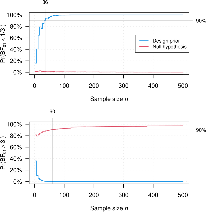
An interesting learning from Table 1 is that to obtain the extremely small sample size of patients of the frequentist power analysis given in Figure 4(b), one must choose a design prior that is even much more informative than pretending to have observed patients already. For the latter, we arrive at Patients. Based on our root-finding approach, using even huge hyperparameters such as and – centered at – yields sample sizes such as under to achieve Bayesian power. This demonstrates that a Bayesian, who is using drastically subjective prior beliefs, is still far away from the small sample size a frequentist is calculating.777A prior based on already observed samples with more than successes would render any subsequent phase II trial with patients entirely obsolete. This can be seen by modification of the results in Figure 4(b) to use the evidence threshold again, which is the one used in the bottom part of Table 1. The results are shown in Figure 4(a).
The top plot in Figure 4(a) demonstrates that samples are required in the power analysis where a point prior is used at – compare Equation 12 – and the results of this frequentist power analysis based on are equal to a Bayesian analysis which assumes patients have already been observed, with failures and successes. Termed otherwise, a frequentist power analysis could be seen with suspicion by almost all Bayesians, whether they choose an objective or subjective prior. From a Bayesian perspective, the required sample size obtained in Figure 4(b) is too optimistically calculated independently of the beliefs about the parameter. However, a frequentist could object that beliefs about the parameter under are irrelevant for power calculations and the sample size should be calculated based on a minimally relevant effect size. Still, a Bayesian could interpret the mode-centered prior under exactly as centered around such a minimally relevant effect, instead of relying on an interpretation in terms of belief.
We close this example by noting that in Table 1, the frequentist type-I-error rate is always larger than the Bayesian averaged type-I-error rate , which is the price paid by the frequentist analysis to achieve larger power FP compared to the Bayesian powers .
Also, the bottom part of Table 1 shows that when shifting to the evidence threshold , the required sample sizes range from to . Note that Bayesian designs with yield a Bayesian type-I-error rate of and are not calibrated anymore. Table 1 shows that shifting to more liberal evidence threshold comes at the price that the smallest sample size which is produced by a calibrated Bayesian design according to Equation 3 is , which still is a reasonable sample size for a phase II proof-of-concept trial that aims at demonstrating the efficacy of a novel drug.
3.2 Therapeutic touch experiment of Rosa et al.
In the second example, we revisit a popular experiment reported by Rosa et al. (1998). Emily Rosa published this study at age nine with the help of her parents, after seeing a television documentary in which so-called therapeutic touch practitioners argued they could sense the human energy field of a person. She tested this supposed ability by letting different practitioners raise their hands through a screen and holding her own hand close to one of the hands. Practitioners then needed to select which of their hands senses Rosa’s human energy field, and Rosa recorded the correct and incorrect decisions from therapeutic touch practitioners. According to Rosa et al. (1998), in the initial trial, the subjects stated the correct location of the investigator’s hand in 70 (47%) of 150 tries.
3.2.1 Priors and hypothesis tests
Two perspectives on a statistical test in the therapeutic touch experiment are possible.
-
First, one could argue to test versus , because it is expected that the proportion of correct decisions by therapeutic touch practitioners should, under absence of any ability to sense a human energy field, be equal to the toss of a fair coin, that is, .
-
Second, one could argue that the ability to sense a human energy field exists only, if therapeutic touch practitioners perform better than the toss of a fair coin. That is, the probability of correct decisions should be larger than , which leads to the test of against .
Both tests can be carried out with the Bayes factors derived in Section 2. For the two-sided test, the Bayes factor in Equation 17 is used, whereas for the directional test, the Bayes factor in Equation 15 is employed.


Figure 6 shows the associated prior and posterior densities for these two testing scenarios. Figure 6(a) shows the prior and posterior for the two-sided test of against in the therapeutic touch experiment, where a flat prior is assigned under .888The prior under is again the limiting case of a prior and reduces to a Dirac measure on , compare Equation 12. The Bayes factor in Equation 17 can be read off the plot by making use of the Savage-Dickey density ratio (Verdinelli and Wasserman, 1995), and is given as the ratio of the ordinates at the blue and red points. The Bayes factor in Equation 17 results in
| (19) |
moderately favouring no effect () over a therapeutic touch effect ().
In comparison, Figure 6(b) and Figure 6(c) show the resulting prior and posterior under respectively , where a truncated prior is used on respectively , compare Equation 10 and Equation 11. Figure 6(d) then shows the plots of Figure 6(b) and Figure 6(c) blended together, which demonstrates that the priors under and yield a prior on the full parameter space . The dashed vertical line in Figure 6(d) illustrates the boundary of the null hypothesis . The resulting Bayes factor for the directional test of the therapeutic touch data results in
| (20) |
moderately favouring no or a negative effect () over a positive effect (, where Equation 17 is used to compute .
While computation of a binomial Bayes factor is straightforward, a sample size calculation in advance of the experiment is helpful to gain some insights about the interpretability of the Bayes factor in terms of Equation 3. In this setting, we aim for and , so we arrive at a Bayesian type-I-error rate of and Bayesian power of at least under the alternative.
3.2.2 Directional test of against
First, we perform the directional test, so the alternative hypothesis specifies that the success probability is larger than , thus and . The shape of the prior distribution for the Bayes factor – in our terms the analysis prior – is specified as the truncated priors under and , shown as the dashed horizontal prior densities in Figure 6(b) and Figure 6(c). Thus,
We use the same truncated Beta priors as our design priors under and , and sample sizes are then calculated via our root-finding approach. The results are shown in Figure 7(a).

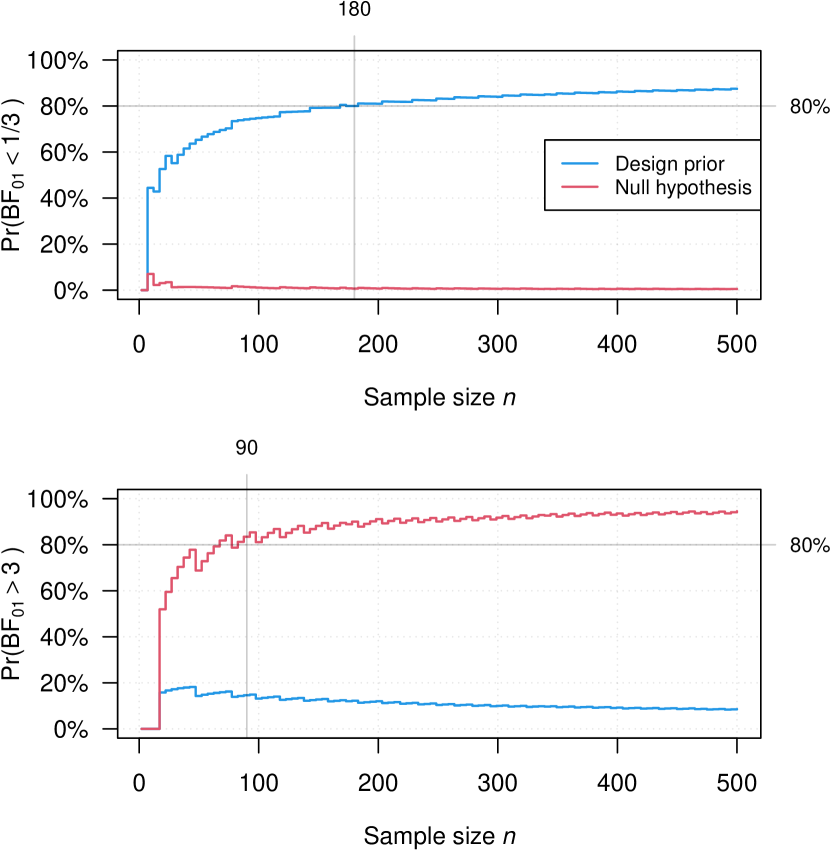
Based on the flat design priors with , participants suffice to attain a power of based on the threshold of strong evidence. The top plot in Figure 6 also shows the type-I-error rate under the null hypothesis as the red solid line, and for we arrive at . Note that as the design and analysis prior coincide by choice here, the power under the analysis prior used for calculation of the Bayes factors would be identical here.
Another relevant point to mention is what happens if a point prior is used for the design prior, so we attain a frequentist type-I-error rate and power as the limiting case of our Beta prior, compare Equation 12. Then, increases to and the design is not calibrated anymore.
Taking stock, Figure 7(a) shows that for a convincing Bayesian analysis based on the Bayes factor with evidence threshold , samples would have sufficed to:
-
Calibrate the design in terms of the Bayesian type-I-error rate for .
-
Calibrate the design in terms of the Bayesian power for .
-
Calibrate the design additionally in terms of the Bayesian probability to find compelling evidence for if indeed holds, that is, for . This is shown in the bottom plot of Figure 7(a), and holds for the same here.999This special case is most probably due to the symmetry of and in combination with the flat design and analysis priors.
We close the discussion of the directional test in the therapeutic touch experiment by noting that the included number of participants could have been reduced to about of the originally used sample size with our approach, compared to the in the therapeutic touch data.
In addition, this example clarifies another important benefit of our root-finding approach: For trials or experiments already carried out with Bayes factors it becomes possible to calculate power and type-I-error rates retrospectively. This allows to gauge the trustworthiness of a Bayesian test in hindsight based on the reported priors and evidence thresholds, or even to recalculate the entire analysis and check whether sample sizes were large enough to provide reliable conclusions. Here, the directional test resulted in a Bayes factor of , compare Equation 20. Thus, the Bayes factor does not pass the threshold . As samples are available in the therapeutic touch experiment and suffice to achieve at least Bayesian power for according to Figure 7(a), the experimental data fail to provide strong evidence for . More importantly, the bottom plot in Figure 7(a) shows that samples also suffice to find compelling evidence for if holds. As the resulting Bayes factor is only , the bottom plot does help little. But we can easily modify the evidence threshold to , to see if our sample size is large enough to warrant the statement that we have found compelling evidence – expressed in terms of a Bayes factor as large as – for the null hypothesis, that is, the absence of a therapeutic touch effect.
Figure 7(b) shows that participants are enough, which is much less than our actually used sample size , compare the therapeutic touch data. Thus, if is convincing enough in terms of evidential strength, we can argue that a retrospective sample size calculation of the experiment of Rosa et al. (1998) demonstrates the absence of any therapeutic touch effect, that is, compelling evidence for .101010If the threshold for moderate evidence is used, the sample sizes shown in Figure 7(b) reduce further to , much less than the available sample size of in the therapeutic touch data. Importantly, this statement is backed by the power and type-I-error guarantees expressed in Equation 3, that is, if there had been a therapeutic touch effect, we had at least power to detect it. Also, the probability of a false-positive result was bounded by .
3.2.3 Two-sided test of against
We turn to the two-sided test in the experiment of Rosa et al. (1998) now. Thus, we test versus and use the prior shown in Figure 6(a). Under , we employ a flat Beta prior, while under , we put a Dirac measure on . The design and analysis priors under are chosen identically as the flat Beta prior, and Figure 8(a) shows the results of the root-finding approach to Bayesian sample size calculation.
Now the required number of participants increases to to attain a Bayesian power of at least . The reason is that now and are less well separated as parameter values slightly larger or smaller than are included in the design prior under . This leads to a larger sample size than in the directional test.
The required sample size to find compelling evidence for shown in the bottom plot of Figure 8(a) increases to samples. Reducing the evidence threshold to yields the results shown in Figure 8(b), and now suffices to attain a Bayesian power of at least under , whereas the probability to find compelling evidence for passes the threshold of at participants, compare the bottom plot in Figure 8(b).
Note that the Bayes factor for the two-sided test resulted in , compare Equation 19. Thus, based both or , the top plots of Figure 8(a) and Figure 8(b) clarify that samples are not enough to achieve Bayesian power for , that is, in favour of a therapeutic touch effect. Also, the bottom plot of Figure 8(a) shows that the sample size of is way too small to be able to demonstrate compelling evidence in favour of based on the strong evidence threshold . However, the bottom plot in Figure 8(b) shows that if the evidence threshold is reduced to , samples suffice to achieve probability to find compelling evidence for the null hypothesis , if indeed holds. As , see the therapeutic touch data, and , the Bayesian sample size calculation in Figure 8(b) demonstrates that the experimental sample size was large enough to find a Bayes factor of at least for with at least probability. From this perspective, a retrospective Bayesian power analysis with our root-finding approach demonstrates that the experiment was designed well enough to interpret the Bayes factor as moderate evidence in favour of . However, as samples would have been necessary for Bayesian power under and only were available, the study was underpowered for when the two-sided test is used.
We can even calculate how large the Bayesian power for e.g. or would have been to achieve a Bayes factor or based on our samples of the therapeutic touch data: The root-finding approach yields , whereas . Thus, the Bayesian power to obtain a Bayes factor respectively was quite large in the experiment. Despite this fact, the experimental data failed to achieve a Bayes factor anywhere close to or . Thus, our root-finding approach clarifies that even in the underpowered setting, the power to find a large enough Bayes factor was quite close to the desired , backing the statement that there is no therapeutic touch effect.111111We stress that these power calculations are based on a flat design prior. If the true effect is very small, perhaps , the study would have been very much underpowered. However, in the state of equipoise about the truth of and , the flat design prior with is a reasonable choice, and the power calculation based on such a prior seems justified.
4 Magic mirror on the wall, which is the best metric of them all?
A key question in the design of experiments is which metric to use to calibrate a design for some statistical test. In Equation 3, we formulated Bayesian analogues to the Neyman-Pearsonian school of thought, where the type-I-error rate is bounded by some and the power is maximized subsequently under . Here, we formulated a bound on the Bayesian type-I-error rate as , and the requirement of at least Bayesian power under as for some . Using this metric comes close to a Bayes-frequentist compromise in the spirit of Good (1983), who argued that the distribution of Bayes factors (under and ) can be used by a frequentist as a test statistic. However, a key advantage of our approach as shown in the examples in Section 3 is that we also can calibrate the probability to find compelling evidence for the null hypothesis . That is, we can design our study to fulfill the bound
| (21) |
for some . For , the latter amounts to design the experiment so that we have a probability of at least to find at least strong evidence in favour of , based on the Bayes factor. As discussed in the phase II clinical trial example, in a variety of situations it might be highly desirable to design a study to have a large probability to find compelling evidence for , if indeed holds. In the bottom part of Figure 1, the three core metrics are shown which are already implemented in the bfpwr package.
In summary, these are:
-
The Bayesian type-I-error rate , where the smallest is calculated by root-finding for which for some , e.g. or .
-
The Bayesian power , where the smallest is calculated by root-finding for which for some , e.g. or .
-
The Bayesian probability of compelling evidence for , , where the smallest is calculated by root-finding for which for some , e.g. or .
We stress that calibrating according to a metric is like a modular system with our root-finding approach: We can calibrate an experimental design according to the Bayesian type-I-error rate, the Bayesian power, the probability to find compelling evidence for the null hypothesis, or combinations thereof. For example, there might be situations where we are only interested in Bayesian power under , and the root-finding approach yields required samples. In another situation, a type-I-error guarantee is required (e.g. due to the requirement for an ethics committee or a trial steering commitee), and the root-finding approach yields required samples now. Taking then yields a design which is calibrated for both aspects.
There might even be different metrics for the Bayes factor – or another test statistic, see the discussion section about possible generalizations of our root-finding approach – that could be of interest and are required to be calibrated. For example, we could interpret indecisive Bayes factors between and as undesirable and formulate the metric
for some , which could be termed as bounding the probability of indecisive evidence under , . Extending our three core metrics to such scenarios and carrying out the root-finding approach is still possible then, although not implemented yet.
We close this section by noting that the answer to the question ’Magic mirror on the wall, which is the best metric of them all?’ depends on the requirements of researchers at the end, our root-finding approach allows for a flexible calibration of a Bayesian design for a variety of metrics which could possibly be of interest in applied research.
5 Discussion
Bayesian design of experiments and sample size calculations usually rely on complex Monte Carlo simulations in practice. Obtaining bounds on Bayesian notions of the false-positive rate and power therefore often lack closed-form or approximate numerical solutions. In this paper, we introduced a novel approach to Bayesian sample size calculation in the binomial setting via Bayes factors. We discussed the drawbacks of sample size calculations via Monte Carlo simulations and proposed a numerical root-finding approach which allows to determine the necessary sample size to obtain prespecified bounds of Bayesian power and type-I-error rate almost instantaneously. Real-world examples and applications in clinical trials illustrated the advantage of the proposed method, where we focussed on point-null versus composite and directional hypothesis tests. We derived the corresponding Bayes factors and discussed relevant aspects to consider when pursuing Bayesian design of experiments with the introduced approach. In summary, our approach allows for a Bayes-frequentist compromise by providing a Bayesian analogue to a frequentist power analysis for the Bayes factor in binomial settings. The methods are implemented in our R package bfpwr121212The binomial test methods are currently only on the development version which can be installed by running remotes::install_github(repo = "SamCH93/bfpwr", subdir = "package", ref = "binomial"), which requires the remotes package. They will soon be made available in the CRAN version of the package, which can be installed with install.packages("bfpwr")..
In this section, we discuss several points which were only addressed briefly and elaborate on extensions and future work in this direction.
5.1 Generalization to other hypothesis testing approaches
An important point not discussed in detail so far is inherent in the workflow depicted in Figure 1: Our root-finding approach is not limited to sample size calculations for Bayes factors. In fact, posterior probabilities could also be used by replacing Equation 16 with
| (22) |
where now has a different interpretation and .The solution can be found by simple numerical methods, and the above clarifies that the root-finding approach is extendable to any statistical test as long as a numerical root-finding method is available. This could become difficult in larger dimensions, but for most statistical tests there exist well-established numerical methods to solve the root in moderately-dimensional parameter spaces.
5.2 Retrospective or reverse-Bayes sample size calculations for Bayes factors
The therapeutic touch experiment discussed in detail in Section 3 clarified another important benefit of our root-finding approach: For trials or experiments already carried out with Bayes factors it becomes possible to calculate power and type-I-error rates retrospectively with our approach. This allows to gauge the trustworthiness of a Bayesian test in hindsight based on the reported priors and evidence thresholds, or even to recalculate the entire analysis and check whether sample sizes were large enough to provide reliable conclusions. A reverse-Bayes analysis in the spirit of Good (1983) is also possible, which answers the question:
Which design prior do we need to achieve a calibrated design?
See also Held et al. (2021) for a review of reverse-Bayes approaches. Another type of retrospective analysis is possible with our method, too, and also based on the detailed discussion of the therapeutic touch example:
How small must the evidence threshold be so that one can accept the resulting Bayes factor in the experiment carried out with sample size as a convincing analysis in the sense that it is based on a calibrated design according to Equation 3?
If one is willing to accept this threshold , an analysis is trustworthy in hindsight. If it is not, the reverse-Bayes analysis casts doubt on the trustworthiness of the carried out experiment. Thus, this second type of retrospective analysis allows to find the evidence threshold for which based on the experimental sample size the design would have been calibrated. Based on the reported Bayes factor one can then check whether , and if so, the analysis is calibrated and trustworthy in hindsight.
5.3 Generalization to other settings
Most importantly, the root-finding approach is not limited to the binomial setting covered in detail in this paper. It is possible to use the same approach for other tests, including tests or tests, compare Pawel and Held (2024) and Wong and Tendeiro (2024). As long as the Bayes factor can be found numerically and a numerical or even analytic solution to Equation 16 is possible, root-finding of the necessary sample size to achieve a prespecified Bayesian power and type-I-error rate should, in general, be possible. The advantage of our approach is obvious in this regard: The sample size calculations require almost no computation time and work almost instantaneously. This is in sharp contrast to the current standard of performing a Monte Carlo simulation study to reveal the required sample size in a given test problem, whether posterior probabilities, Bayes factors or posterior odds are the chosen test criterion.
Proofs
Proof.
Expectation of a truncated beta random variable
Let be a beta random variable truncated to the interval from to , i.e., . The expectation of is
| (23) |
where the last equality follows from Pascal’s identity. ∎
Derivation of the prior-predictive probability mass function.
First, the prior-predictive is given by definition as
| (24) |
and from
| (25) |
it follows by substituting Equation 25 in Equation 24 that
| (26) |
which is Equation 14. ∎
Derivation of the Bayes factor for the one-sided test of versus for .
By definition, the Bayes factor is given as
| (27) |
Based on the truncated Beta analysis prior, compare Equation 10 and Equation 11, the predictive probability mass functions under and are given as
| (28) |
and
| (29) |
so
| (30) | ||||
| (31) |
From
the right-hand side of Equation Equation 31 simplifies further to
| (33) | |||
| (34) |
The numerator of Equation 34 can be written as
| (35) |
and the denominator in Equation 34 can be written as
| (36) |
and therefore Equation 34 simplifies further to
| (37) |
and the right-hand side of Equation 37 yields Equation 15 and finishes the proof. ∎
Derivation of the Bayes factor for the two-sided test of versus .
Based on the same assumption , a Dirac measure in is chosen as the analysis prior under , that is,
. A Beta analysis prior is chosen under , that is,
with hyperparameters . Based on these analysis priors under and , we have
| (38) | ||||
| (39) | ||||
| (40) | ||||
| (41) |
where the right-hand side of Equation 41 yields Equation 17. ∎
Relationship of and for mode-centered Beta design priors.
Let be a beta random variable, then the mode is given as for , or as any value in the domain of for . Let be given for some in , then
| (42) | |||
So for any , selection of as specified above yields a mode-centered Beta random variable. As the mode is invariant under truncation, because each density value is normalized only with a multiplicative constant, this also holds for the truncated Beta design priors. ∎
Mean- and mode-centering for a Beta random variable.
Now, the mean of a Beta random variable is given as , and from
| (43) |
for some from , we obtain
| (44) |
Substitution of the latter in Equation 42 yields
| (45) |
which proves that mean- and mode-centering is possible only when . Note that while the mean changes when truncating the Beta design priors, the mode stays invariant, so the proof also works when using the expectation of the truncated Beta distribution, because the multiplicative constant in the right-hand side of Equation 23 only modifies the resulting value for . ∎
References
- \NAT@swatrue
- D. A. Berry (2006) Berry, D. A. (2006, 2). Bayesian clinical trials. Nature Reviews Drug Discovery 2006 5:1, 5, 27-36. doi: 10.1038/nrd1927 \NAT@swatrue
- S. M. Berry (2011) Berry, S. M. (2011). Bayesian adaptive methods for clinical trials. CRC Press. \NAT@swatrue
- Bijma et al. (2017) Bijma, F., Jonker, M., and van der Vaart, A. (2017). Introduction to mathematical statistics. Amsterdam University Press. \NAT@swatrue
- Brown et al. (2001) Brown, L. D., Cai, T. T., and Gupta, A. D. (2001, 5). Interval estimation for a binomial proportion. Statistical Science, 16, 101-133. doi: 10.1214/SS/1009213286 \NAT@swatrue
- Dawid (1982) Dawid, A. P. (1982). The well-calibrated Bayesian. Journal of the American Statistical Association, 77, 605-610. doi: 10.1080/01621459.1982.10477856 \NAT@swatrue
- Depaoli and van de Schoot (2017) Depaoli, S., and van de Schoot, R. (2017, 6). Improving transparency and replication in Bayesian statistics: The wambs-checklist. Psychological Methods, 22, 240-261. doi: 10.1037/MET0000065 \NAT@swatrue
- Good (1960) Good, I. (1960). Weight of evidence, corroboration, explanatory power, information and the utility of experiments. Journal of the Royal Statistical Society: Series B (Methodological), 22, 319-331. doi: 10.1111/J.2517-6161.1960.TB00378.X \NAT@swatrue
- Good (1983) Good, I. (1983). Good thinking: The foundations of probability and its applications. Minneapolis University Press. \NAT@swatrue
- Grieve (2016) Grieve, A. P. (2016, 3). Idle thoughts of a ’well-calibrated’ Bayesian in clinical drug development. Pharmaceutical statistics, 15, 96-108. doi: 10.1002/PST.1736 \NAT@swatrue
- Grieve (2022) Grieve, A. P. (2022). Hybrid frequentist/Bayesian power and Bayesian power in planning and clinical trials. Chapman & Hall, CRC Press. \NAT@swatrue
- Held et al. (2021) Held, L., Matthews, R., Ott, M., and Pawel, S. (2021). Reverse-Bayes methods for evidence assessment and research synthesis. Research Synthesis Methods. doi: 10.1002/JRSM.1538 \NAT@swatrue
- Held and Sabanés Bové (2014) Held, L., and Sabanés Bové, D. (2014). Applied statistical inference. Springer. doi: 10.1007/978-3-642-37887-4 \NAT@swatrue
- Jeffreys (1939) Jeffreys, H. (1939). Theory of probability (1st ed.). The Clarendon Press. \NAT@swatrue
- Julious (2023) Julious, S. A. (2023, 1). Sample sizes for clinical trials, second edition. Sample Sizes for Clinical Trials, Second Edition, 1-396. doi: 10.1201/9780429503658 \NAT@swatrue
- Kelter (2020a) Kelter, R. (2020a). Analysis of Bayesian posterior significance and effect size indices for the two-sample t-test to support reproducible medical research. BMC Medical Research Methodology, 20. doi: 10.1186/s12874-020-00968-2 \NAT@swatrue
- Kelter (2020b) Kelter, R. (2020b). Bayesian survival analysis in stan for improved measuring of uncertainty in parameter estimates. Measurement: Interdisciplinary Research and Perspectives, 18, 101-119. doi: 10.1080/15366367.2019.1689761 \NAT@swatrue
- Kelter (2021a) Kelter, R. (2021a). Analysis of type I and II error rates of Bayesian and frequentist parametric and nonparametric two-sample hypothesis tests under preliminary assessment of normality. Computational Statistics, 36, 1263-1288. doi: 10.1007/s00180-020-01034-7 \NAT@swatrue
- Kelter (2021b) Kelter, R. (2021b). Bayesian Hodges-Lehmann tests for statistical equivalence in the two-sample setting: Power analysis, type I error rates and equivalence boundary selection in biomedical research. BMC Medical Research Methodology, 21. doi: 10.1186/s12874-021-01341-7 \NAT@swatrue
- Kelter (2021c) Kelter, R. (2021c). How to choose between different Bayesian posterior indices for hypothesis testing in practice. Multivariate Behavioral Research, 1-29. doi: 10.1080/00273171.2021.1967716 \NAT@swatrue
- Kelter (2021d) Kelter, R. (2021d, 5). Type I and II error rates of Bayesian two-sample tests under preliminary assessment of normality in balanced and unbalanced designs and its influence on the reproducibility of medical research. Journal of Statistical Computation and Simulation, 91. doi: 10.1080/00949655.2021.1925278 \NAT@swatrue
- Kelter (2022) Kelter, R. (2022). The evidence interval and the Bayesian evidence value – on a unified theory for Bayesian hypothesis testing and interval estimation. British Journal of Mathematical and Statistical Psychology, 75, 550-592. doi: https://doi.org/10.1111/bmsp.12267 \NAT@swatrue
- Kelter (2023) Kelter, R. (2023). The Bayesian simulation study (basis) framework for simulation studies in statistical and methodological research. Biometrical Journal, 2200095. doi: 10.1002/BIMJ.202200095 \NAT@swatrue
- Kelter and Schnurr (2024) Kelter, R., and Schnurr, A. (2024, 4). The Bayesian group-sequential predictive evidence value design for phase II clinical trials with binary endpoints. Statistics in Biosciences, 1-37. doi: 10.1007/s12561-024-09430-z \NAT@swatrue
- Kerridge (1963) Kerridge, D. (1963, 9). Bounds for the frequency of misleading Bayes inferences. The Annals of Mathematical Statistics, 34, 1109-1110. doi: 10.1214/AOMS/1177704038 \NAT@swatrue
- Kleijn (2022) Kleijn, B. (2022). The frequentist theory of Bayesian statistics. Springer. \NAT@swatrue
- Kruschke (2014) Kruschke, J. K. (2014). Doing Bayesian data analysis: A tutorial with r, jags, and stan (2nd ed.). Academic Press. doi: 10.1016/B978-0-12-405888-0.09999-2 \NAT@swatrue
- Kruschke (2021) Kruschke, J. K. (2021, 8). Bayesian analysis reporting guidelines. Nature Human Behaviour 2021 5:10, 5, 1282-1291. doi: 10.1038/s41562-021-01177-7 \NAT@swatrue
- Kruschke and Vanpaemel (2015) Kruschke, J. K., and Vanpaemel, W. (2015). Bayesian estimation in hierarchical models. The Oxford Handbook of Computational and Mathematical Psychology, 279-299. doi: 10.1093/oxfordhb/9780199957996.013.13 \NAT@swatrue
- Lee and Liu (2008) Lee, J., and Liu, D. D. (2008). A predictive probability design for phase ii cancer clinical trials. Clinical Trials, 5, 93-106. doi: 10.1177/1740774508089279 \NAT@swatrue
- Little (2006) Little, R. J. (2006, 8). Calibrated Bayes: A Bayes/frequentist roadmap. The American Statistician, 60, 213-223. doi: 10.1198/000313006X117837 \NAT@swatrue
- Makowski et al. (2019) Makowski, D., Ben-Shachar, M. S., Chen, S. H. A., and Lüdecke, D. (2019). Indices of effect existence and significance in the Bayesian framework. Frontiers in Psychology, 10, 2767. doi: 10.3389/fpsyg.2019.02767 \NAT@swatrue
- Matthews (2006) Matthews, J. N. (2006). Introduction to randomized controlled clinical trials (2nd ed.). CRC Press. \NAT@swatrue
- Morris et al. (2019) Morris, T. P., White, I. R., and Crowther, M. J. (2019, 5). Using simulation studies to evaluate statistical methods. Statistics in Medicine, 38, 2074-2102. doi: 10.1002/SIM.8086 \NAT@swatrue
- O’Hagan and Stevens (2001) O’Hagan, A., and Stevens, J. (2001). Bayesian assessment of sample size for clinical trials of cost-effectiveness. Medical Decision Making, 21(3), 219–230. doi: 10.1177/02729890122062514 \NAT@swatrue
- Pawel and Held (2024) Pawel, S., and Held, L. (2024, 6). Closed-form power and sample size calculations for Bayes factors. arXiv preprint. Retrieved from https://arxiv.org/abs/2406.19940v2 \NAT@swatrue
- Pourmohamad and Wang (2023) Pourmohamad, T., and Wang, C. (2023). Sequential Bayes factors for sample size reduction in preclinical experiments with binary outcomes. Statistics in Biopharmaceutical Research, 15, 706-715. doi: 10.1080/19466315.2022.2123386 \NAT@swatrue
- Robert and Casella (2004) Robert, C., and Casella, G. (2004). Monte Carlo statistical methods. Springer. \NAT@swatrue
- Rosa et al. (1998) Rosa, L., Rosa, E., Sarner, L., and Barrett, S. (1998, 4). A close look at therapeutic touch. JAMA, 279, 1005-1010. doi: 10.1001/JAMA.279.13.1005 \NAT@swatrue
- Rosner (2021) Rosner, G. L. (2021). Bayesian thinking in biostatistics. Chapman and Hall/CRC. \NAT@swatrue
- Rubin (1984) Rubin, D. B. (1984). Bayesianly justifiable and relevant frequency calculations for the applied statistician. The Annals of Statistics, 12, 1151-1172. \NAT@swatrue
- Santis (2004) Santis, F. D. (2004, 8). Statistical evidence and sample size determination for Bayesian hypothesis testing. Journal of Statistical Planning and Inference, 124, 121-144. doi: 10.1016/S0378-3758(03)00198-8 \NAT@swatrue
- Schönbrodt and Wagenmakers (2018) Schönbrodt, F. D., and Wagenmakers, E. J. (2018, 2). Bayes factor design analysis: Planning for compelling evidence. Psychonomic Bulletin and Review, 25, 128-142. doi: 10.3758/S13423-017-1230-Y/FIGURES/5 \NAT@swatrue
- Schönbrodt et al. (2017) Schönbrodt, F. D., Wagenmakers, E.-J., Zehetleitner, M., and Perugini, M. (2017). Sequential hypothesis testing with Bayes factors: Efficiently testing mean differences. Psychological Methods., 22, 322-339. Retrieved from doi:10.1037/met0000061 \NAT@swatrue
- Stefan et al. (2019) Stefan, A. M., Gronau, Q. F., Schönbrodt, F. D., and Wagenmakers, E.-J. (2019). A tutorial on Bayes factor design analysis using an informed prior. Behavior Research Methods, 51(3), 1042–1058. doi: 10.3758/s13428-018-01189-8 \NAT@swatrue
- Stefan et al. (2022) Stefan, A. M., Schönbrodt, F. D., Evans, N. J., and Wagenmakers, E. J. (2022, 3). Efficiency in sequential testing: Comparing the sequential probability ratio test and the sequential Bayes factor test. Behavior Research Methods, 1-18. doi: 10.3758/S13428-021-01754-8 \NAT@swatrue
- Team (2020) Team, R. C. (2020). R: A language and environment for statistical computing. R Foundation for Statistical Computing. Retrieved from https://www.r-project.org/ \NAT@swatrue
- U.S. Food and Drug Administration (2010) U.S. Food and Drug Administration. (2010). Guidance for the use of Bayesian statistics in medical device clinical trials. Retrieved from https://www.fda.gov/regulatory-information/search-fda-guidance-documents/guidance-use-bayesian-statistics-medical-device-clinical-trials \NAT@swatrue
- Van de Schoot et al. (2021) Van de Schoot, R., Depaoli, S., King, R., Kramer, B., Märtens, K., Tadesse, M. G., … Yau, C. (2021, 1). Bayesian statistics and modelling. Nature Reviews Methods Primers 2021 1:1, 1, 1-26. doi: 10.1038/s43586-020-00001-2 \NAT@swatrue
- Verdinelli and Wasserman (1995) Verdinelli, I., and Wasserman, L. (1995). Computing Bayes factors using a generalization of the Savage-Dickey density ratio. Journal of the American Statistical Association, 90, 614-618. doi: 10.1080/01621459.1995.10476554 \NAT@swatrue
- Wang and Gelfand (2002) Wang, F., and Gelfand, A. E. (2002, 5). A simulation-based approach to Bayesian sample size determination for performance under a given model and for separating models. Statistical Science, 17, 193-208. doi: 10.1214/SS/1030550861 \NAT@swatrue
- Weiss (1997) Weiss, R. (1997, 7). Bayesian sample size calculations for hypothesis testing. Journal of the Royal Statistical Society: Series D (The Statistician), 46, 185-191. doi: 10.1111/1467-9884.00075 \NAT@swatrue
- Wong and Tendeiro (2024) Wong, T. K., and Tendeiro, J. (2024, 9). On a generalizable approach for sample size determination in Bayesian t tests. psyArXiv preprint. Retrieved from https://osf.io/6h4d5 doi: 10.31234/OSF.IO/6H4D5 \NAT@swatrue
- H. Zhou et al. (2017) Zhou, H., Lee, J. J., and Yuan, Y. (2017, 9). Bop2: Bayesian optimal design for phase II clinical trials with simple and complex endpoints. Statistics in Medicine, 36, 3302-3314. doi: 10.1002/SIM.7338 \NAT@swatrue
- T. Zhou and Ji (2023) Zhou, T., and Ji, Y. (2023, 1). On Bayesian sequential clinical trial designs. The New England Journal of Statistics in Data Science, 2(1), 136–151. doi: 10.51387/23-NEJSDS24