Cantor sets in higher dimensions   I:
criterion for stable intersections

Abstract.

We study the geometry of dynamically defined Cantor sets in arbitrary dimensions, introducing a criterion for $\mathcal{C}^{1+\alpha}$ stable intersections of such Cantor sets, under a mild bunching condition. This condition is naturally satisfied for perturbations of conformal Cantor sets and, in particular, always holds in dimension one. Our work extends the celebrated recurrent compact set criterion of Moreira and Yoccoz for stable intersection of Cantor sets in the real line to higher-dimensional spaces. Based on this criterion, we develop a method for constructing explicit examples of stably intersecting Cantor sets in any dimension. This construction operates in the most fragile and critical regimes, where the Hausdorff dimension of one of the Cantor sets is arbitrarily small and both Cantor sets are nearly homothetical. All results and examples are provided in both real and complex settings.

1. Introduction

Cantor sets appear naturally in many dynamical systems as the invariant sets. Despite all being homeomorphic, Cantor sets may exhibit drastically different geometric features in the ambient space.

Over the past five decades, a deep connection between the fractal geometry of regular (or dynamically defined) Cantor sets and the bifurcation theory of diffeomorphisms (mostly in dimension two) has been unveiled by Newhouse, Palis, Takens, Yoccoz, Moreira and Viana, among others, [17], [19], [25], [26], [27], [28], [10], [6], [22], [29], [14]. In his pioneering works [15] and [16], Newhouse introduced the concept of thickness for Cantor sets in the real line and demonstrated the stable intersection of thick regular Cantor sets, as the milestone of the creation of Newhouse phenomenon [17] for surface diffeomorphisms. Recall that a Cantor set is regular if it can be generated as the unique attractor of the iterated function systems of a finite family of smooth contracting maps. Also, in brief words, two regular Cantor sets $K,K^{\prime}$ have $\mathcal{C}^{r}$ stable intersection if $\tilde{K}$ intersects $\tilde{K}^{\prime}$ for any pair of Cantor sets $\tilde{K},\tilde{K}^{\prime}$ whose generating maps are sufficiently $\mathcal{C}^{r}$-close to those of $K,K^{\prime}$, respectively (see §2). A central problem in this direction is the following.

Problem 1.1.

Under what conditions does a pair of regular Cantor sets exhibit stable intersection?

Moreira and Yoccoz [13] have developed a remarkable criterion for the stable intersection of Cantor sets in the real line. A family of renormalization operators on a suitable function space was associated with a given pair of regular Cantor sets ($K$, $K^{\prime}$), for which it was shown that the existence of a recurrent compact set implies $\mathcal{C}^{1+\alpha}$ stable intersection of $K$ and $K^{\prime}$. This allowed them to address Problem 1.1 for all typical Cantor sets in the real line, proving a strong form of Palis Conjecture [21] (See also [31]).

In the complex setting, Buzzard [6] has extended Newhouse’s results by creating a pair of stably intersecting Cantor sets in $\mathbb{C}$. Buzzard’s approach, however, relied on different mechanisms, specifically leveraging the good isotropy properties of the conformal maps that generate these Cantor sets. The Newhouse’s criterion (gap lemma) has been recently extended to regular Cantor sets in $\mathbb{C}$ by Biebler [5] under some extra assumptions. See also [32].

Recently, Araujo, Moreira and Zamudio [1], [2] extended the method introduced in [13] to the complex setting, proving a criterion for the stable intersection of regular (conformal) Cantor sets in $\mathbb{C}$ and extend the Moreira-Yoccoz theorem to conformal Cantor sets in $\mathbb{C}$ with large Hausdorff dimension. Their results establish that stability holds within the space of holomorphic (conformal) maps. A Cantor set $K$ is called conformal (resp. homothetical) if the derivative of its generating maps are orthonormal (resp. homothety) on $K$. In dimension one, real or complex, regular Cantor sets are all homothetical (and so conformal) by definition.

In higher dimensions very little is known. The only known examples of stable intersection of a pair of Cantor sets in $\mathbb{R}^{d}$ ($d>1$), are given by Asaoka [3]. Those examples are based on a purely higher dimensional phenomenon that appears in blenders [4] (see also [12], [18]). This yields pairs of Cantor sets $(K,K^{\prime})$ in $\mathbb{R}^{d}$ ($d\geq 2$) exhibiting $\mathcal{C}^{1}$ stable intersections. Such pairs of Cantor sets exhibit a distinctive geometry and are far from being conformal, as their generators satisfy a domination property essential for applying the blender mechanism. Furthermore, this phenomenon implies that both Cantor sets must have Hausdorff dimensions greater than one, thereby restricting it to higher-dimensional settings. Specifically, it requires that $\lfloor\operatorname{dim_{HD}}(K)\rfloor+\lfloor\operatorname{dim_{HD}}(K^{\prime})\rfloor\geq d$, where $\lfloor t\rfloor$ is the integer part of $t$. Notably, the $\mathcal{C}^{1}$ stability of intersections does not occur for any pair of Cantor sets on the real line [11]. This indicates that a universal scenario may not be conceivable for all dimensions and raises numerous questions.

The aim of this work is to address the challenge of identifying a general criterion for the stable intersection of Cantor sets in all dimensions, both in the real and complex settings. A key step towards this goal is to obtain a fine analysis of the geometry of regular Cantor sets at arbitrarily small scales. It is achieved in $\mathcal{C}^{1+\alpha}$ regularity and under a mild bunching condition (Theorem 4.9). This bounded geometry result may be of independent interest and shed some light on the poorly understood geometry of Cantor sets in higher dimensions. The bunching condition here is always satisfied in dimension one and also applies to perturbations of conformal Cantor sets in higher dimensions. Building on this, we establish a criterion for $\mathcal{C}^{1+\alpha}$ stable intersections of regular Cantor sets in arbitrary dimensions (real or complex).

Relying on our criterion, we present a method for constructing explicit examples of $\mathcal{C}^{1+\alpha}$ stably intersecting Cantor sets in $\mathbb{R}^{d}$ (see §7). This construction operates in the most fragile and critical regimes, where the Hausdorff dimension of one of the Cantor sets is arbitrarily small and both Cantor sets are nearly homothetical. In particular, we have the following.

Theorem A.

For every $d\in\mathbb{N}$, $\alpha\in(0,1)$ and $\epsilon>0$, there exists a pair of Cantor sets $(K,K^{\prime})$ in $\mathbb{R}^{d}$ with $\mathcal{C}^{1+\alpha}$ stable intersection such that $\dim_{\rm{HD}}(K)<\epsilon$. Moreover, the Cantor sets $K,K^{\prime}$ may be affine and arbitrarily close to the space of conformal (or homothetical) Cantor sets.

Here, as in the one-dimensional setting, $\mathcal{C}^{1+\alpha}$ regularity plays a crucial role. In fact, in a forthcoming paper [20], extending the work of Moreira [11] to higher dimensions, we demonstrate that for the examples of Thoerem A (where $\operatorname{dim_{HD}}(K)<1$) the intersection of $K$ and $K^{\prime}$ cannot exhibit $\mathcal{C}^{1}$ stability. Thus, despite some conjectures in [3], we propose the following problem, for which we expect a positive answer.

Problem 1.2.

Let $(K,K^{\prime})$ be a pair of regular Cantor sets in $\mathbb{R}^{d}$ satisfying

$$\lfloor\operatorname{dim_{HD}}(K)\rfloor+\lfloor\operatorname{dim_{HD}}(K^{\prime})\rfloor<d.$$

Is it always possible to vanish their intersection by a $\mathcal{C}^{1}$ small perturbation?

Remark 1.3.

Note that the sum of Hausdorff dimensions of the Cantor sets in Theorem A is smaller than $d+\epsilon$. On the other hand, a necessary condition for the stable intersection is that the sum of Hausdorff dimensions be bigger than $d$.

Our method applies also in the complex setting. So, we have a similar statement for holomorphic Cantor sets in $\mathbb{C}^{d}$.

Theorem B.

For every $d\in\mathbb{N}$ and $\epsilon>0$, there exists a pair of holomorphic Cantor sets $(K,K^{\prime})$ in $\mathbb{C}^{d}$ with stable intersection in the holomorphic topology such that $\dim_{\rm{HD}}(K)<\epsilon$. Moreover, the Cantor sets $K,K^{\prime}$ may be affine and arbitrarily close to the conformal (or homothetical) Cantor sets.

1.1. The criterion

One can induce a family of renormalization operators corresponding to a pair of regular Cantor sets $(K,K^{\prime})$, which acts on some infinite dimensional space $\mathcal{Q}$ representing relative $\mathcal{C}^{1+\alpha}$ embeddings of $K$ and $K^{\prime}$ in the ambient space $\mathbb{R}^{d}$. Indeed, any pair $[h,h^{\prime}]\in\mathcal{Q}$ represents the class of all $\mathcal{C}^{1+\alpha}$ embeddings $(A\circ h)(K),(A\circ h^{\prime})(K^{\prime})$ in $\mathbb{R}^{d}$ of $K,K^{\prime}$, where $A\in\operatorname{\rm{Aff}}(d,\mathbb{R})$ and $h,h^{\prime}$ are $\mathcal{C}^{1+\alpha}$ maps on $\mathbb{R}^{d}$. Here, $\operatorname{\rm{Aff}}(d,\mathbb{R})$ is the space of invertible affine maps of $\mathbb{R}^{d}$. Roughly speaking, the renormalization operators zoom in to the smaller parts of regular Cantor sets. The key property here is that small parts of regular Cantor sets are geometrically similar to the entire Cantor set. Moreover, they keep some finite dimensional space $\mathcal{Q}_{\operatorname{\rm{Aff}}}\subset\mathcal{Q}$ invariant. It turns out that $\mathcal{Q}_{\operatorname{\rm{Aff}}}$ represents the relative affine infinitesimal structure of the pair of Cantor sets and $\mathcal{Q}_{\operatorname{\rm{Aff}}}\cong\operatorname{\rm{Aff}}(d,\mathbb{R})\times\Sigma^{-}\times\Sigma^{\prime-}$, where $\Sigma^{-},\Sigma^{\prime-}$ are one sided shift spaces corresponding to the dynamical definitions of $K,K^{\prime}$. Analogously, in the holomorphic case we study the action of renormalization operators on certain infinite dimensional space $\mathcal{Q}^{\rm Hol}$ and its finite dimensional invariant subspace $\mathcal{Q}_{\operatorname{\rm{Aff}}}^{\rm Hol}\cong\operatorname{\rm{Aff}}(d,\mathbb{C})\times\Sigma^{-}\times\Sigma^{\prime-}$. For precise definitions we refer to Section 2 and Section 5.

Figure 1. A Cantor set generated by four affine maps: initial approximations.

In the case that the generating maps of the Cantor sets $K$ and $K^{\prime}$ are affine maps, the action of renormalization operators can be simplified as follows. In this case renormalization operators are the pairs $(X,X^{\prime})$ that act on $\operatorname{\rm{Aff}}(d,\mathbb{R})$ by

$$H\mapsto X^{-1}\circ H\circ X^{\prime},$$

where $(X,X^{\prime})$ is either $(\mathrm{Id},R^{\prime})$ or $(R,\mathrm{Id})$, and $R,R^{\prime}$ are affine generators of $K,K^{\prime}$, respectively.

Theorem C (Covering criterion for stable intersection).

Let $d\in\mathbb{N}$, and $(K,K^{\prime})$ be a pair of bunched Cantor sets in $\mathbb{R}^{d}$ with the corresponding family $\mathcal{R}$ of renormalization operators. Assume that there exists a bounded open set $\mathcal{U}\subset\mathcal{Q}_{\operatorname{\rm{Aff}}}$ satisfying the covering condition

(1.1) $$\overline{\mathcal{U}}\subset\bigcup_{\Psi\in\mathcal{R}}\Psi^{-1}(\mathcal{U}).$$

Then the Cantor sets $h(K)$ and $h^{\prime}(K^{\prime})$ have $\mathcal{C}^{1+\alpha}$ stable intersection for all $[h,h^{\prime}]\in\mathcal{U}$. In particular, if $[\mathrm{Id},\mathrm{Id}]\in\mathcal{U}$ then $K$ and $K^{\prime}$ have $\mathcal{C}^{1+\alpha}$ stable intersection.

Note that the condition (1.1) is finite dimensional, while the conclusion holds $\mathcal{C}^{1+\alpha}$-stably in the infinite dimensional space of regular Cantor sets.

Theorem C extends to the complex setting and for holomorphic Cantor sets.

Theorem D.

Let $d\in\mathbb{N}$, and $(K,K^{\prime})$ be a pair of bunched holomorphic Cantor sets in $\mathbb{C}^{d}$ with the corresponding family $\mathcal{R}$ of renormalization operators. Assume that there exists a bounded open set $\mathcal{U}\subset\mathcal{Q}_{\operatorname{\rm{Aff}}}^{\rm Hol}$ satisfying the covering condition (1.1). Then $h(K)$ and $h^{\prime}(K^{\prime})$ have stable intersection for all $[h,h^{\prime}]\in\mathcal{U}$. In particular, if $[\mathrm{Id},\mathrm{Id}]\in\mathcal{U}$ then $K$ and $K^{\prime}$ have stable intersection. The stability holds in the space of holomorphic maps.

Remark 1.4.

For the Cantor set on the real line, covering condition (1.1) is equivalent to the recurrent compact set criterion in the work of Moreira and Yoccoz [13]. In particular, Theorems C and D generalize the recurrent compact set criterion of [13] and [1], respectively.

A number of applications of these results are expected, though not discussed in this paper, particularly in the bifurcation theory of diffeomorphisms in arbitrary dimensions, the global dynamics of group actions on diffeomorphisms, their ergodic properties, and related topics.

1.2. About the proofs

The general strategy of the proof of Theorem C is similar to the work of Moreira-Yoccoz [13]. However, to generalize their renormalization method to higher dimensions, one needs to deal with the non-conformal behavior of typical maps. First, we need to analyze the infinitesimal geometry of regular Cantor sets. Thus, a main part of the proof is devoted to the convergence of limit geometries for the sequences of contracting maps in arbitrary dimensions. Such convergence results crucially require a bunching condition and also the $\mathcal{C}^{1+\alpha}$ regularity. Fine geometric control under iterated contracting maps, as studied in [7], addresses the behavior of balls under iterations of sequences of contracting $\mathcal{C}^{1+\alpha}$ maps with a quasi-conformality condition (QC) [7, Definition 2.2]. Here, we broaden this geometric control to encompass any sequence of contracting maps satisfying a bunching condition (see Definition 2.3). This condition yields the bounded geometry (Theorem 4.9) and holds in various settings, including sequences of contracting maps in the vicinity of conformal contracting maps. This type of assumptions appears in many other contexts in dynamical systems (e.g. in stable ergodicity, regularity of holonomy maps, etc.) as well as in other areas of mathematics. On the other hand, as we discussed in Remark 6.7, the affine case automatically verifies the bounded geometry. Thus, it remains a big challenge to understand infinitesimal geometry and the intersection of Cantor sets violating the bunching condition.

To prove Theorems A and B, presenting examples of stably intersecting Cantor sets in arbitrary dimensions, we apply the covering criterion in Theorems C and D, respectively. To verify the covering criterion in higher dimensions, we adapt and utilize the ideas and methods introduced in [7]. The other ingredient of our construction is inspired by the examples of affine stably intersecting Cantor sets on the real line developed in [23] and [24] (see §7.1).

Organization

In Section 2, basic notations and definitions are established, including the bunching condition for regular Cantor sets. In Section 3, we discuss the abstract covering condition on any metric space. In Section 4, we prove the control of shape property for a sequence of bunched contracting local diffeomorphisms in $\mathbb{R}^{d}$. Then we focus on the main object of study: Cantor sets at infinitesimal scales, also known as limit geometries. Section 5 defines renormalization operators and studies them on affine Cantor sets as special cases. The covering criterion, which is the main result of this paper, is proved in Section 6. In Section 7, we develop a method to verify the covering criterion, specifically proving Theorems A and B.

Acknowledgement

The authors express their gratitude to Federico Rodriguez Hertz, Carlos Gustavo Moreira, Enrique Pujals and Reza Seyyedali for their fruitful comments and conversations. Special thanks are extended to Mehdi Pourbarat for his valuable critiques and discussions throughout this work. The authors also thank ICTP for its support and hospitality, where parts of this work were written.

2. Preliminaries

2.1. Basic notations

Here we fix some basic notations that we will use in the rest of the paper frequently.

• We may use the notation $\mathbb{F}$ as either $\mathbb{R}$ or $\mathbb{C}$ when both cases can be described in a same way.

• We denote the Hausdorff dimension of the set $A\subset\mathbb{R}^{d}$ as $\operatorname{dim_{HD}}(A)$.

• We denote $\mathrm{O}(d)$ as the group of orthonormal linear transformations over $\mathbb{R}^{d}$.

• Given a metric space $(X,d)$, for any $x\in X$ we denote the $\delta$-neighborhood of $x$ in $X$ as $B_{\delta}(x)$. For $V\subset X$ we define $B_{\delta}(V):=\bigcup_{v\in V}B_{\delta}(v)$ and $V_{(\delta)}:=\{v\in V:\;B_{\delta}(v)\subset V\}$.

• Given compact sets $A,B\subset\mathbb{R}^{d}$, denote $\operatorname{\rm{dist}}(A,B):=\min_{x\in A,\;y\in B}{|x-y|}$.

• Denote the space of invertible matrices over $\mathbb{F}^{d}$ by $\operatorname{\rm{GL}}(d,\mathbb{F})$ and those with determinant equal to $1_{\mathbb{F}}$ as $\operatorname{\rm{SL}}(d,\mathbb{F})$. For $A\in\operatorname{\rm{GL}}(d,\mathbb{F})$ we denote its norm by $\|A\|_{\it op}:=\sup_{|v|=1}|Av|$ and its co-norm by $m(A):=\inf_{|v|=1}|Av|$.

• We denote by $\operatorname{\rm{Aff}}(d,\mathbb{F})$ the space of invertible affine transformations $[x\mapsto Ax+a]$ of $\mathbb{F}^{d}$ equipped with $\mathcal{C}^{1}$ topology where $A\in\operatorname{\rm{GL}}(d,\mathbb{F})$ and $a\in\mathbb{F}^{d}$.

• We denote the identity matrix in $\operatorname{\rm{GL}}(d,\mathbb{F})$ as $\mathrm{Id}$. We also use the notation $\mathrm{Id}$ for the identity function. Each case will be clear in the context.

• $\operatorname{\rm{GL}}(d,\mathbb{C})$ can be interpreted as a subgroup of $\operatorname{\rm{GL}}(2d,\mathbb{R})$ since any $T=A+iB\in\operatorname{\rm{GL}}(d,\mathbb{C})$ with $A,B\in M(d,\mathbb{R})$ maps a vector $x+iy\in\mathbb{C}^{d}$ where $x,y\in\mathbb{R}^{d}$ to the vector $(Ax-By)+i(Bx+Ay)$. Therefore, $T$ acts as a linear map on $\mathbb{R}^{2d}$ which sends the vector $(x,y)\in\mathbb{R}^{2d}$ to $(Ax-By,Bx+Ay)\in\mathbb{R}^{2d}$ and $A,B$ are such that this mapping is not singular. This implies that $\operatorname{\rm{Aff}}(d,\mathbb{C})$ is a subgroup of $\operatorname{\rm{Aff}}(2d,\mathbb{R})$.

• (Hölder regularity) The $\mathcal{C}^{\alpha}$ semi-norm, $\mathcal{C}^{1}$ norm and $\mathcal{C}^{1+\alpha}$ norm of an $\mathcal{C}^{1+\alpha}$ map $f:X\to\mathbb{R}^{d}$ on the domain $U\subset X$ are defined, respectively by

  $$\|f\|_{\mathcal{C}^{0}} :=\sup_{u\in U}|f(u)|,$$

  $$|f|_{\alpha} :=\sup_{x,y\in U}\frac{|f(x)-f(y)|}{d(x,y)^{\alpha}},$$

  $$\|f\|_{\mathcal{C}^{1}} :=\|f\|_{\mathcal{C}^{0}}+\sup_{u\in U}\|Df(u)\|_{\it op},$$

  $$\|f\|_{\mathcal{C}^{1+\alpha}} :=\|f\|_{\mathcal{C}^{1}}+|Df|_{\alpha}.$$

• We denote by $\operatorname{\rm{Diff}}^{r}_{\rm loc}(M)$, the space of all $\mathcal{C}^{r}$ diffeomorphisms $f:\mathrm{Dom}(f)\to\mathrm{Im}(f)$ such that $\mathrm{Dom}(f)$, $\mathrm{Im}(f)$ are open subsets of $M$. $f,g\in\operatorname{\rm{Diff}}^{r}_{\rm loc}(M)$ are $\mathcal{C}^{r}$-close if there exists a diffeomorphism $h:\mathrm{Dom}(f)\to\mathrm{Dom}(g)$ $\mathcal{C}^{r}-$close to $\mathrm{Id}|_{\mathrm{Dom}(f)}$ such that the map $g\circ h$ is $\mathcal{C}^{r}$-close to $f$. In other words, two elements of $\operatorname{\rm{Diff}}_{\rm loc}^{r}(M)$ are $\mathcal{C}^{r}$-close if their graphs are $\mathcal{C}^{r}$-close embedded submanifolds of $M\times M$.

2.2. Regular Cantor sets

In this subsection we define regular Cantor sets in $\mathbb{R}^{d}$ (or $\mathbb{R}^{2d}\cong\mathbb{C}^{d}$). We keep the notations similar to the ones used in [1].

Definition 2.1.

A regular (or dynamically defined) Cantor set in $\mathbb{R}^{d}$ is defined by the following data:

• A finite set $\mathfrak{A}$ of letters and a set $\mathfrak{B}\subset\mathfrak{A}\times\mathfrak{A}$ of admissible pairs.

• For each $a\in\mathfrak{A}$ a compact connected set $G(a)\subset\mathbb{R}^{d}$. In the complex case $G(a)$ is a compact subset of $\mathbb{R}^{2d}\cong\mathbb{C}^{d}$.

• A $\mathcal{C}^{1+\alpha}$ map $g:V\to\mathbb{R}^{d}$ defined in an open neighborhood $V$ of $\bigsqcup_{a\in\mathfrak{A}}G(a)$. In the complex case $g$ maps $V$ into $\mathbb{R}^{2d}\cong\mathbb{C}^{d}$.

This data must verify the following assumptions:

• The sets $G(a)$, $a\in\mathfrak{A}$ are pairwise disjoint

• $(a,b)\in\mathfrak{B}$ implies $G(b)\subset g(G(a))$, otherwise $G(b)\cap g(G(a))=\emptyset$.

• For each $a\in\mathfrak{A}$ the restriction $g|_{G(a)}$ can be extended to a $\mathcal{C}^{1+\alpha}$ embedding (with $\mathcal{C}^{1+\alpha}$ inverse) from an open neighborhood of $G(a)$ onto its image such that $m(Dg):=\inf\{m(Dg(x)):x\in V\}>\mu^{-1}$ for some positive constant $\mu<1$. In the complex case $Dg(x)$ is a member of $\operatorname{\rm{GL}}(2d,\mathbb{R})$ for all $x\in V$.

• The subshift $(\Sigma_{\mathfrak{B}},\sigma)$ is called the symbolic type of the Cantor set

  (2.1) $$\Sigma_{\mathfrak{B}}:=\{{\underline{a}}=(a_{0},a_{1},a_{2},\dots)\in\mathfrak{A}^{\mathbb{N}}:(a_{i},a_{i+1})\in\mathfrak{B},\;\text{for all}\;i\geq 0\}$$

  with the topologically mixing shift map $\sigma(a_{0},a_{1},a_{2},\dots):=(a_{1},a_{2},a_{3},\dots)$.

Once we have all these data we can define a Cantor set (i.e. a nonempty, perfect, compact and totally disconnected set) on $\mathbb{R}^{d}$ (or $\mathbb{R}^{2d}\cong\mathbb{C}^{d}$),

$$K=\bigcap_{n\geq 0}g^{-n}\left(\bigsqcup_{a\in\mathfrak{A}}G(a)\right).$$

We say that $K$ is a Cantor set described by the data $(\Sigma_{\mathfrak{B}},g)$. Whenever the set $\mathfrak{B}$ is fixed and clear from the context we simply say that $K$ is constructed via $(\Sigma,g)$.

Remark 2.2.

Note that here we defined regular Cantor sets with an expanding generator. We also could define them with contracting generators which are inverse of the expanding generator $g$ restricted to domains $G(a)$. Sometimes we will use this definition of regular Cantor sets. More precisely, given contracting maps $f_{i}:\overline{U}\to G(a_{i})$ for $i=1,\dots,m$ where $m:=\#\mathfrak{A}$, $a_{i}\in\mathfrak{A}$ and $\overline{U}\subset\mathbb{R}^{d}$ is a compact set, the maximal invariant set of the Iterated Function System (IFS) generated by $f_{1},\dots,f_{m}$ with the symbolic type $\Sigma$ is the regular Cantor set $K$. In that case we say that the regular Cantor set $K$ is generated by the Iterated Function Systems $\{f_{1},\dots,f_{k}\}$ and the subshift $(\Sigma,\sigma)$. In the case that $(\Sigma,\sigma)$ is the full shift dynamics we say that the Cantor set $K$ is constructed via the IFS $\{f_{1},\dots,f_{m}\}$.

A regular Cantor set $K$ may be constructed in many ways as described above. For instance, the standard middle third Cantor set may be constructed via both $(\Sigma_{\mathfrak{B}_{i}},g_{i})$, where $\mathfrak{A}_{1}:=\{1,2\}$, $\mathfrak{A}_{2}:=\{1,2,3,4\}$, $\mathfrak{B}_{i}=\mathfrak{A}_{i}\times\mathfrak{A}_{i}$ for $i=1,2$ and

$$g_{1}:\bigcup_{j=0,2}\left[\frac{j}{3},\frac{j+1}{3}\right]\to[0,1],\qquad g_{2}:\bigcup_{j=0,1,3,4}\left[\frac{2j}{9},\frac{2j+1}{9}\right]\to[0,1],$$

such that $g_{1}(x)=3x-j$ for $x\in[\frac{j}{3},\frac{j+1}{3}]$ and $g_{2}(x)=9x-2j$ for $x\in[\frac{2j}{9},\frac{2j+1}{9}]$. Therefore, when we say that $K$ is a regular Cantor set we assume a set of data $(\Sigma_{\mathfrak{B}},g)$ is fixed. For convenience, we will just mention this set of data most of the times by the expanding map $g$ since all the data can be inferred if we know $g$ or by an IFS of contracting generators as we explained above.

2.3. Bunched Cantor Sets

Definition 2.3.

Given a regular Cantor set $K$ in $\mathbb{R}^{d}$ described by $(\Sigma_{\mathfrak{B}},g)$ where $g$ is a $\mathcal{C}^{1+\alpha}$ map with a uniform expansion rate bigger than $\mu^{-1}>1$, we say that $K$ is

• affine if for any $a\in\mathfrak{A}$, $g|_{G(a)}:G(a)\to\mathbb{R}^{d}$ is an expanding affine map.

• homothetical if $Dg(x)/\|Dg(x)\|_{\it op}=\mathrm{Id}$ for all $x\in K$,

• conformal if $Dg(x)/\|Dg(x)\|_{\it op}\in\operatorname{O}(d)$ for all $x\in K$,

• bunched whenever $g$ is bunched at the Cantor set $K$, that is, there is $N_{g}\in\mathbb{N}$ such that for all $x\in K$, $Dg(x)\in\operatorname{\rm{GL}}(d,\mathbb{R})$ and

  (2.2) $$\|Dg^{N_{g}}(x)\|_{\textit{op}}\cdot\|Dg^{N_{g}}(x)^{-1}\|_{\textit{op}}\cdot\mu^{\alpha\cdot N_{g}}<1.$$

• holomorphic if $d$ is an even integer and for any $x\in K$, $Dg(x)$ lies in $\operatorname{\rm{GL}}(d/2,\mathbb{C})$ which is a subgroup of $\operatorname{\rm{GL}}(d,\mathbb{R})$.

Remark 2.4.

For convenience and in order to make the presentation as transparent as possible we assume that $N_{g}=1$ throughout the paper. This is not an essential restriction because by using an adapted metric one can assume that $N_{g}=1$ in (2.2).

Remark 2.5.

Conformal Cantor sets are special cases of bunched (or bunched holomorphic) Cantor sets. Conformal Cantor sets in $\mathbb{R}^{2}$ are defined in [1] to analyze regular Cantor sets appear in $\mathbb{C}$. Note that any holomorphic Cantor set in $\mathbb{R}^{2}$ is bunched and coincides with conformal Cantor sets. Moreover, the bunching condition always holds in a neighborhood of conformal Cantor sets. Therefore, small perturbations of conformal Cantor sets are bunched (holomorphic) Cantor sets.

Given a regular Cantor set $K$ generated by $g$, $K$ is the maximal invariant compact subset of $\mathbb{R}^{d}$. Indeed, the pair $(K,g|_{K})$ is a dynamical system which is conjugate to the subshift $\Sigma_{\mathfrak{B}}$. The conjugacy map $h:K\to\Sigma$ is a homeomorphism that maps each $x\in K$ to the sequence of letters $\{a_{n}\}_{n\geq 0}$ gained by the orbit of $x$. In particular, $g^{n}(x)\in G(a_{n})$ for all $n$. Associated to the Cantor set $K$ we define the sets

$$\Sigma^{\mathrm{fin}} :=\{(a_{0},\dots,a_{n}):n\in\mathbb{N},\;(a_{i},a_{i+1})\in\mathfrak{B}\;\text{for all}\;i,\;0\leq i<n\},$$

$$\Sigma^{-} :=\{(\dots,a_{-n},a_{-n+1},\dots,a_{-1},a_{0}):(a_{i-1},a_{i})\in\mathfrak{B}\;\text{for all}\;i\leq 0\}.$$

Given ${\underline{a}}=(a_{0},\dots,a_{n})\in\Sigma^{\rm fin}$ we say that the length of ${\underline{a}}$ is $n$. For $\underline{\theta}=(\dots,\theta_{-2},\theta_{-1},\theta_{0})\in\Sigma^{-}$ where $\theta_{0}=a_{0}$ and $\underline{b}=(b_{0},b_{1},\dots)$ we denote

$$\underline{\theta a} :=(\dots,\theta_{-2},\theta_{-1},a_{0},\dots,a_{n}),$$

$$\underline{b}_{k} :=(b_{0},b_{1},\dots,b_{k}),$$

$$\underline{\theta}_{k} :=(\theta_{-k},\dots,\theta_{-1},\theta_{0})$$

for all $k$. Furthermore, we define the set

$$G({\underline{a}}):=\{x\in\bigsqcup_{a\in\mathfrak{A}}G(a),g^{j}(x)\in G(a_{j}),j=0,1,\dots,n\}$$

and the map $f_{{\underline{a}}}:G(a_{n})\to G({\underline{a}})$ by

$$f_{{\underline{a}}}:=\left(g|^{-1}_{G(a_{0})}\circ g|^{-1}_{G(a_{1})}\circ\dots\circ g|^{-1}_{G(a_{n-1})}\right)\Big{|}_{G(a_{n})}.$$

Notice that $f_{(a_{i},a_{i+1})}=g|^{-1}_{G(a_{i})}$, so we have

$$f_{{\underline{a}}}=f_{(a_{0},a_{1})}\circ f_{(a_{1},a_{2})}\circ\cdots\circ f_{(a_{n-1},a_{n})}.$$

This implies that the finite collection of maps $\{f_{(a,b)}\;|\;(a,b)\in\mathfrak{B}\}$ generates the family $\{f_{{\underline{a}}}\}_{{\underline{a}}\in\Sigma^{\rm fin}}$ by their composition through the set $\Sigma$. Therefore, $K$ will be the attractor of the IFS generated by this family through to the symbolic type $\Sigma$.

Notice that in the definition of regular Cantor set $K$, pieces $G(a)$ may have empty interior. However, we can replace pieces $G(a)$ with open relatively compact connected pieces $G^{*}(a):=B_{\delta}(G(a))$ for sufficiently small $\delta>0$ and extend the map $g|_{(G(a)}$ to the neighborhood of $G^{*}(a)$ for all $a\in\mathfrak{A}$ such that the pieces $\overline{G^{*}(a)}$ and the map $g$ satisfy the properties enumerated in the Definition 2.1. Let also

$$G^{*}({\underline{a}}):=\{x\in\bigsqcup_{a\in\mathfrak{A}}G^{*}(a),g^{j}(x)\in G^{*}(a_{j}),j=0,1,\dots,n\}.$$

With this notation, we have the following lemma from [1, Lemma 2.1].

Lemma 2.6.

Let $K$ be a regular Cantor set and $G^{*}(a)$ the sets defined above. There exists a constant $C>0$ such that

$$\operatorname{\rm{diam}}(G^{*}({\underline{a}}))<C\mu^{n},$$

where $\mu<1$ is such that $m(Dg)>\mu^{-1}$ in $\bigsqcup_{a\in\mathfrak{A}}G^{*}(a)$ and ${\underline{a}}=(a_{0},\dots,a_{n})$.

Lemma 2.6 implies that substitution of the pieces $G(a)$ by $G^{*}(a)$ will not change the Cantor set $K$ since $G({\underline{a}})\subset G^{*}({\underline{a}})$ and diam$(G^{*}({\underline{a}}))\rightarrow 0$. So, we may consider all of the pieces $G(a)$ be compact sets which are the closure of their interiors.

Definition 2.7.

Let $\beta>1$ an $\Sigma:=\Sigma_{\mathfrak{B}}$ be a symbolic type defined by a given $\mathfrak{A},\mathfrak{B}$ as (2.1). We denote $\Omega_{\Sigma,d}^{\beta}$ as the set of all bunched Cantor sets $K$ in $\mathbb{R}^{d}$ described by the data $(\Sigma,g)$ where $g$ is a $\mathcal{C}^{\beta}$ map. We equip $\Omega_{\Sigma,d}^{\beta}$ with the topology generated by $\delta$-neighborhoods $U_{K,\delta}$ of $K\in\Omega_{\Sigma,d}^{\beta}$. Each $U_{K,\delta}$ consists of bunched Cantor sets $K^{\prime}$ with symbolic type $\Sigma$ generated by some $\mathcal{C}^{\beta}$ map $g^{\prime}$ with pieces $G^{\prime}(a)$ with the property that $g^{\prime}|_{G^{\prime*}(a)}$ is $\delta$-close to $g|_{G^{*}(a)}$ in $\operatorname{\rm{Diff}}^{\beta}_{\rm loc}(\mathbb{R}^{d})$, for all $a\in\mathfrak{A}$. In the holomorphic case, we denote the set of all bunched holomorphic Cantor sets in $\mathbb{R}^{2d}$ with a topology on it in the same manner and denote it by $\Omega^{\operatorname{\rm{Hol}},\beta}_{\Sigma,2d}$.

Remark 2.8.

Notice that the bunching condition (2.2) for a Cantor set is stable in the $\mathcal{C}^{1+\alpha}$ topology for $\alpha>0$.

3. The covering conditions

Given a family of maps $\mathcal{F}$, we denote $\left\langle{\mathcal{F}}\right\rangle^{+}$ as a semigroup generated by $\mathcal{F}$.

Definition 3.1 (Covering condition).

Let $\mathcal{F}$ be a family of continuous maps on a metric space $(X,d)$. We say that a set $V\subset X$ satisfies the covering condition with respect to $\mathcal{F}$ if

(3.1) $$\overline{V}\subset\bigcup_{f\in\mathcal{F}}f^{-1}(V).$$

This condition implies that for any $v\in\overline{V}$ there is $f\in\mathcal{F}$ such that $f(v)\in V$. In other words, one can map any $v\in\overline{V}$ into $V$ by one iteration of the elements of $\mathcal{F}$.

Definition 3.2 (Strong covering condition).

Let $\mathcal{F}$ be a finite family of continuous maps on a metric space $(X,d)$. We say that a set $V\subset X$ satisfies the strong covering condition with respect to $\mathcal{F}$ if there exists $\delta>0$ such that

(3.2) $$B_{\delta}(V)\subset\bigcup_{f\in\mathcal{F}}f^{-1}(V_{(\delta)}).$$

The following two lemmas are direct consequences of continuity argument and the proofs are omitted.

Lemma 3.3.

For a finite family $\mathcal{F}$ of continuous maps on a locally compact metric space $(X,d)$, the covering condition implies strong covering condition for an open relatively compact set $V\subset X$.

Given a finite family $\mathcal{F}=\{f_{1},\ldots,f_{k}\}$ of continuous maps, we say that the family $\tilde{\mathcal{F}}$ is $\epsilon$-close to $\mathcal{F}$ in the $\mathcal{C}^{0}$ topology, if $\tilde{\mathcal{F}}=\{\tilde{f}_{1},\ldots,\tilde{f}_{k}\}$ is such that $f_{i},\tilde{f}_{i}$ are $\epsilon$-close in the $\mathcal{C}^{0}$ topology for $i=1,\ldots,k$.

Lemma 3.4 (Stability of strong covering).

Let $\mathcal{F}$ be a finite family of continuous maps on a metric space $(X,d)$ and $V\subset X$ be a subset that satisfies strong covering condition with respect to $\mathcal{F}$. Then for any family $\tilde{\mathcal{F}}$ sufficiently close to $\mathcal{F}$ in $\mathcal{C}^{0}$ topology, $V$ satisfies strong covering condition with respect to $\tilde{\mathcal{F}}$.

In the following lemma we make a bridge from (strong) covering condition with respect to a family $\mathcal{F}$ to the (strong) covering condition with respect to its generated semigroup $\left\langle{\mathcal{F}}\right\rangle^{+}$.

Lemma 3.5.

Let $\mathcal{F}$ be a finite family of uniformly continuous maps on the metric space $(X,d)$ such that an open set $V\subset X$ satisfies strong covering with respect to a finite family $\mathcal{F}^{\prime}\subset\left\langle{\mathcal{F}}\right\rangle^{+}$. Then, there exists $W\subset X$ containing $V$ and satisfying strong covering condition with respect to $\mathcal{F}$.

Proof.

Let $\mathcal{F}:=\{f_{1},\cdots,f_{k}\}$. By the assumptions there are $\epsilon>0$, $N\in\mathbb{N}$, such that for any $v\in B_{\epsilon}(V)$ there exists a word $\underline{w}=(w_{n},\dots,w_{2},w_{1})\in\{1,\dots,k\}^{n}$ with $n<N$ such that $B_{\epsilon}(f_{\underline{w}}(v))\subset V$ where, $f_{\underline{w}}:=f_{w_{n}}\circ\cdots\circ f_{w_{2}}\circ f_{w_{1}}$. Since elements of the finite family $\mathcal{F}$ are uniformly continuous then there exist positive real numbers $\delta_{0},\delta_{1},\dots,\delta_{N}<\epsilon$ such that for every $i\in\{1,\dots,N\}$, $f\in\mathcal{F}$ and $x,y\in X$, if $d(x,y)<\delta_{i-1}$ then $d(f(x),f(y))<\delta_{i}/4$. We also denote

(3.3) $$\delta:=\dfrac{1}{2}\min\{\delta_{0},\delta_{1},\dots,\delta_{n}\}.$$

Fixing $v\in B_{\epsilon}(V)$, then there is $\underline{w}=(w_{n},\dots,w_{1})$ such that $B_{\epsilon}(f_{\underline{w}}(v))\subset V$. Now let $v_{0}:=v$, $W_{0}:=B_{\delta_{0}}(v)$ and $v_{i}:=f_{w_{i}}(v_{i-1})$, $W_{i}:=B_{\delta_{i}}(v_{i})$ for $i\in{1,2,\dots,N}$. It follows from the properties of $\delta_{i}$’s that $B_{\epsilon/2}(W_{n})\subset V$. In particular, by (3.3) we have $B_{\delta}(f_{w_{i}}(B_{\delta}(W_{i-1})))\subset W_{i}$ for $i\in\{1,2,\dots,n\}$. So if we define $U_{v}:=\bigcup_{i=0}^{N}W_{i}$ then $W:=\bigcup_{v\in V}U_{v}$ has strong covering condition. More precisely,

$$B_{\delta}(W)\subset\bigcup_{f\in\mathcal{F}}f^{-1}(W_{(\delta)}).$$

∎

Remark 3.6.

This proof shows that if $V$ is open relatively compact then one can assume continuity of elements of the finite family $\mathcal{F}$ instead of uniform continuity.

3.1. Covering in linear groups

In the rest of this section we will study group operation of Lie groups $\operatorname{\rm{SL}}(d,\mathbb{F})$, for $\mathbb{F}$ being either $\mathbb{R}$ or $\mathbb{C}$. Here, we recall covering condition for left action of elements of such a group. Assuming $G$ is a topological group, let $\mathcal{F}\subset G$ be a set of elements of this group. We say that $\mathcal{U}\subset G$ satisfies covering condition with respect to $\mathcal{F}$ if

(3.4) $$\overline{\mathcal{U}}\subset\bigcup_{f\in\mathcal{F}}f^{-1}\mathcal{U},$$

where $f^{-1}\mathcal{U}=\{f^{-1}u:u\in\mathcal{U}\}$. By Lemma 3.3, $\mathcal{U}$ being open relatively compact implies that the covering condition is equivalent to the strong covering. We use both real and complex versions of [7, Lemma 3.8]. Proof of its complex version is analogous to the real case with the same computations in scalar field $\mathbb{C}$ instead of $\mathbb{R}$.

Lemma 3.7.

Let $\mathcal{U}_{0}$, $\mathcal{U}_{1}$ be neighborhoods of $\mathrm{Id}$ in $\operatorname{\rm{SL}}(d,\mathbb{F})$. Then, there exists an open relatively compact set $\mathcal{U}\subseteq\mathcal{U}_{0}$ and a finite set $\mathcal{F}\subset\mathcal{U}_{1}$ such that $\mathcal{U}$ satisfies strong covering condition with respect to $\mathcal{F}$. Moreover, $\mathcal{F}$ has at most $1+\dim(\operatorname{\rm{SL}}(d,\mathbb{F}))$ elements.

4. Convergent geometries

An important tool for study the infinitesimal parts of a regular Cantor set is the convergence of geometries. Roughly speaking, it says that given a sequence of smooth contracting maps satisfying a bunching condition (which always holds in dimension 1, either real or complex), the tail of their composition behaves like the composition of contracting affine maps.

4.1. Existence and continuity of limits

For a sequence $\{h_{n}\}_{n\in\mathbb{N}}$ we denote $h^{n}:=h_{n}\circ\cdots\circ h_{1}$. Given $\rho,C>0$ and $\mu,\mu^{\prime},\alpha\in(0,1)$ and $\kappa\geq 1$, we consider the following hypotheses for a sequence of maps $\{h_{n}\}_{n\in\mathbb{N}}$ in $\operatorname{\rm{Diff}}^{1+\alpha}_{\rm loc}(\mathbb{R}^{d})$.

• $h_{n}:B_{\rho}(0)\rightarrow h_{n}(B_{\rho}(0))$ is a $\mathcal{C}^{1+\alpha}$ diffeomorphism fixing the origin,

• $\|h_{n}\|_{\mathcal{C}^{1+\alpha}}<C$,

• (uniform contraction) for any $y\in B_{\rho}(0)$, $\mu^{\prime}<\|Dh_{n}(y)\|_{\textit{op}}<\mu$,

• (bunching) there is $N>0$ such that $\|Dh^{n}(0)\|_{\textit{op}}\cdot\|(Dh^{n}(0))^{-1}\|_{\textit{op}}<\mu^{-n\alpha}$ for all $n\geq N$.

For the convenience and to make the presentation more straightforward, we may replace the hypothesis (H3) above with the following slightly stronger one throughout the paper.

• $\|Dh_{n}(0)\|_{\textit{op}}\cdot\|(Dh_{n}(0))^{-1}\|_{\textit{op}}\leq\kappa<\mu^{-\alpha}$.

Theorem 4.1 (Convergence of geometries).

Let $C,\rho>0$ and $\mu^{\prime},\mu,\alpha\in(0,1)$ and $\kappa\geq 1$ be real numbers. Let $\{f_{i}\}_{i\in\mathbb{N}}$ be a sequence in $\operatorname{\rm{Diff}}^{1+\alpha}_{\rm loc}(\mathbb{R}^{d})$ satisfying (H0)-(H3). Then, the sequence $\{(Df^{n}(0))^{-1}\circ f^{n}\}_{n\in\mathbb{N}}$ converges in $\operatorname{\rm{Diff}}^{1+\alpha}_{\rm loc}(\mathbb{R}^{d})$ to some $F:B_{\rho}(0)\to\mathbb{R}^{d}$. Moreover, the convergence is uniformly exponential for every sequence satisfying (H0)-(H3) and the limit depends uniformly $\mathcal{C}^{1}$-continuously on the sequence $\{f_{n}\}_{n\in\mathbb{N}}$.

Here, by the uniform continuity of the limit we mean that for any $\varepsilon>0$ there is $\delta>0$ such that given two sequences $\{f_{n}\}_{n\in\mathbb{N}}$ and $\{\tilde{f}_{n}\}_{n\in\mathbb{N}}$ satisfying (H0)-(H3) with $\max\{d_{\mathcal{C}^{1+\alpha}}(f_{n},\tilde{f}_{n}):n=1,2,\dots\}<\delta$, then their limits are $\varepsilon$-close in $\operatorname{\rm{Diff}}^{1+\alpha}_{\rm loc}(\mathbb{R}^{d})$.

In further sections we will use this theorem to obtain infinitesimal properties of regular Cantor sets. Using $\mathcal{C}^{0}$-convergence in this theorem one can deduce the following control of shape property.

Corollary 4.2 (Control of shape).

Let $C,\rho>0$ and $\mu^{\prime},\mu,\alpha\in(0,1)$ and $\kappa\geq 1$ be real numbers. Then there exist $\xi_{0}>0$ and $\eta_{1}>1>\eta_{2}$ such that for every sequence $\{f_{i}\}_{i\in\mathbb{N}}$ in $\operatorname{\rm{Diff}}^{1+\alpha}_{\rm loc}(\mathbb{R}^{d})$ satisfying (H0)-(H3), $\xi\in(0,\xi_{0}]$ and $n\in\mathbb{N}$,

(4.1) $$\eta_{2}\cdot L_{n}(B_{\xi}(0))\subseteq f^{n}(B_{\xi}(0))\subseteq\eta_{1}\cdot L_{n}(B_{\xi}(0)),$$

where $L_{n}:=Df^{n}(0)$ is the derivative of $f^{n}$ at $0$.

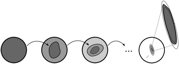
Figure 2. Sequence of maps satisfying (H0)-(H3) in Corollary 4.2, where the iterations of small balls remain almost ellipsoids.

Remark 4.3.

This corollary yields the control of shape property in [7]. Indeed, [7, Theorem 4.5] assumes quasi-conformality of the sequence $\{f^{n}\}_{n\in\mathbb{N}}$ at the origin, which implies our assumptions (H3) and (H3^′) for the sequence $\{g_{n}\}_{n\in\mathbb{N}}$, where $g_{n}:=f_{nk}\circ\cdots\circ f_{nk-k+1}$ for a sufficiently large integer $k$.

Remark 4.4.

The condition (H2) is always satisfied in the study of the geometry of regular Cantor sets. However, within the proof of Theorem 4.1 it turns out that we could consider the following more general condition (H2^′) instead of (H2):

• there is a sequence of numbers $\{\mu^{\prime}_{n}\}_{n=1}^{\infty}$ in $(0,1)$ with $\lim_{n\to\infty}\frac{1}{n}\ln\mu^{\prime}_{n}=0$ such that for all $n\in\mathbb{N}$ and any $y\in B_{\rho}(0)$, $\mu^{\prime}_{n}<\|Dh_{n}(y)\|_{\textit{op}}<\mu$.

Proof of Theorem 4.1.

Let $r_{n}$ be the diameter of $U_{n}$, where $U_{n}:=f^{n}\left(B_{\rho}(0)\right)$ for $n\in\mathbb{N}$ and $U_{0}:=B_{\rho}(0)$. Since $f_{n}$ is a contracting map with uniform contraction rate $\mu<1$ on $U_{n-1}$, we have $\operatorname{\rm{diam}}(U_{n})\leq\mu\cdot\operatorname{\rm{diam}}(U_{n-1})$. Therefore, $r_{n}\leq\rho\cdot\mu^{n}$. Let $A_{k}=Df_{k}(0)$, then $Df^{n}(0)=A_{n}\circ A_{n-1}\circ\cdots\circ A_{1}.$ We can define

(4.2) $$F_{n}:=(Df^{n}(0))^{-1}\circ f^{n}=A_{1}^{-1}\circ\cdots\circ A_{n}^{-1}\circ f_{n}\circ\cdots\circ f_{1}.$$

We have to prove that $\{F_{n}\}_{n\geq 1}$ is convergent in $\mathcal{C}^{1+\alpha}$ topology on $B_{\rho}(0)$. For any $z,v\in B_{\rho}(0)$ such that $z+v\in B_{\rho}(0)$ we have

(4.3) $$\left|f_{n}(z+v)-\left(f_{n}(z)+Df_{n}(z)\cdot v\right)\right|<C\cdot|v|^{1+\alpha}.$$

Consequently, $f_{n}$ is $C\cdot r_{n-1}^{1+\alpha}$ close to the map $A_{n}$ in $\mathcal{C}^{0}$ norm on $U_{n-1}$. Thus, if $n$ is large enough by (4.3) we have

$$r_{n}\leq\|A_{n}\|_{\textit{op}}\cdot r_{n-1}+C\cdot r^{1+\alpha}_{n-1}\leq r_{n-1}\cdot\big{(}\|A_{n}\|_{\textit{op}}+C_{1}\cdot\mu^{(n-1)\alpha}\big{)},$$

where $C_{1}:=C\cdot\rho^{\alpha}$. Arguing by induction, using the inequality $\log(x+y)\leq\log x+\frac{y}{x}$ (for positive real numbers $x,y$), we obtain

$$\log r_{n}\leq\log\prod_{k=1}^{n}\|A_{k}\|_{\textit{op}}+C_{0}\cdot\sum_{j=0}^{n-1}(C_{1}\cdot\mu^{j\alpha})\leq\log\prod_{k=1}^{n}\|A_{k}\|_{\textit{op}}+C_{2},$$

where $C_{0}:=\sup_{i\geq 1}\|Df_{i}(0)\|_{\textit{op}}^{-1}<1/{\mu^{\prime}}$ and $C_{2}=\dfrac{C_{0}\cdot C_{1}}{1-\mu^{\alpha}}$. So $r_{n}\leq C_{3}\cdot\prod_{k=1}^{n}\|A_{k}\|_{\textit{op}},$ where $C_{3}:=\exp(C_{2})$. Analogously using the inequality $\log(x-y)\geq\log x-\frac{y}{x-y}$ (for $0<y<x$), we can show, possibly by enlarging $C_{3}$ , that

$$C_{3}^{-1}\cdot\prod_{k=1}^{n}m(A_{k})\leq r_{n}\leq C_{3}\cdot\prod_{k=1}^{n}\|A_{k}\|_{\textit{op}},$$

which means that the size of $f^{n}(B_{\rho}(0))$ is controlled. This with (4.3) implies that

(4.4) $$\|g_{n}\|_{\mathcal{C}^{0}}=\left\|f_{n}-A_{n}\right\|_{\mathcal{C}^{0}}\leq C\cdot r_{n-1}^{1+\alpha}\leq C_{4}\prod_{k=1}^{n-1}\|A_{k}\|_{\textit{op}}^{1+\alpha},$$

where $g_{k}$ is $f_{k}-A_{k}$ and $C_{4}:=C\cdot C_{3}^{1+\alpha}$ and the $\mathcal{C}^{0}$ norm is calculated inside the domain $f^{n}(B_{\rho}(0))$. By (4.2) and (4.4) we have

$$F_{n}=\bigg{(}\mathrm{Id}+A_{1}^{-1}\circ\cdots\circ A_{n}^{-1}\circ g_{n}\circ A_{n-1}\circ\cdots\circ A_{1}\bigg{)}\circ F_{n-1}.$$

Therefore, $F_{n}$ is a sequence of composition of functions

$$F_{n}=(\mathrm{Id}+S_{n})\circ(\mathrm{Id}+S_{n-1})\circ\cdots\circ(\mathrm{Id}+S_{1}),$$

where $S_{n}:=A_{1}^{-1}\circ\cdots\circ A_{n}^{-1}\circ g_{n}\circ A_{n-1}\circ\cdots\circ A_{1}.$ We will observe that $S_{n}$ has exponentially small $\mathcal{C}^{1+\alpha}$ norm. We have

$$\|S_{n}\|_{\mathcal{C}^{0}} \leq\prod_{k=1}^{n}\|A_{k}^{-1}\|_{\textit{op}}\cdot\|g_{n}\|_{\mathcal{C}^{0}}$$

$$\leq C_{4}\cdot\prod_{k=1}^{n}\|A_{k}^{-1}\|_{\textit{op}}\cdot\prod_{k=1}^{n-1}\|A_{k}\|_{\textit{op}}^{1+\alpha}$$

$$\leq C_{4}\cdot C_{0}^{1+\alpha}\cdot\kappa^{n}\cdot\prod_{k=1}^{n}\|A_{k}\|_{\textit{op}}^{\alpha}$$

(4.5) $$\leq C_{5}\cdot(\kappa\cdot\mu^{\alpha})^{n},$$

where $C_{5}:=C_{4}\cdot C_{0}^{1+\alpha}$. We also have the following estimate for $\|DS_{n}\|_{\it op}$ on $B_{\rho}(0)$.

$$\|DS_{n}\|_{\textit{op}} =\|A_{1}^{-1}\circ\cdots\circ A_{n}^{-1}\circ Dg_{n}\circ A_{n-1}\circ\cdots\circ A_{1}\|_{\textit{op}}$$

$$\leq\prod_{i=1}^{n}\|A_{i}^{-1}\|_{\textit{op}}\cdot\|Dg_{n}\|_{\textit{op}}\cdot\prod_{i=1}^{n-1}\|A_{i}\|_{\textit{op}}$$

$$\leq C_{0}\cdot\kappa^{n}\cdot\|Dg_{n}\|_{\textit{op}}$$

(4.6) $$\leq C_{6}\cdot(\kappa\cdot\mu^{\alpha})^{n},$$

where $C_{6}:=C_{0}\cdot C\cdot(\rho\mu^{-1})^{\alpha}$ and the last inequality comes from $\alpha$-Hölder regularity of $Df_{n}$, that for any $z\in U_{n-1}$ we have

$$\|Dg_{n}(z)\|_{\textit{op}}=\|Df_{n}(z)-Df_{n}(0)\|_{\textit{op}}\leq C\cdot r_{n-1}^{\alpha}\leq C\cdot(\rho\mu^{-1})^{\alpha}\cdot\mu^{n\alpha}.$$

We can also bound the $\alpha$ - Hölder semi norm $|DS_{n}|_{\alpha}$ as below

$$|DS_{n}|_{\alpha} =\sup_{a_{0},b_{0}\in U_{0}}\dfrac{\|DS_{n}(a_{0})-DS_{n}(b_{0})\|_{\textit{op}}}{|a_{0}-b_{0}|^{\alpha}}$$

$$=\sup_{a_{0},b_{0}\in U_{0}}\dfrac{1}{|a_{0}-b_{0}|^{\alpha}}\cdot\|A_{1}^{-1}\circ\cdots\circ A_{n}^{-1}$$

$$\qquad\qquad\qquad\qquad\qquad\circ(Dg_{n}(a_{n-1})-Dg_{n}(b_{n-1}))\circ A_{n-1}\circ\cdots\circ A_{1}\|_{\textit{op}}$$

$$\leq\sup_{a_{0},b_{0}\in U_{0}}\dfrac{1}{|a_{0}-b_{0}|^{\alpha}}\cdot\prod_{i=1}^{n}\|A_{i}^{-1}\|_{\textit{op}}\cdot\|Dg_{n}(a_{n-1})-Dg_{n}(b_{n-1})\|_{\textit{op}}\cdot\prod_{i=1}^{n-1}\|A_{i}\|_{\textit{op}}$$

$$\leq\sup_{a_{0},b_{0}\in U_{0}}\dfrac{C_{0}\cdot\kappa^{n}}{|a_{0}-b_{0}|^{\alpha}}\cdot\|Dg_{n}(a_{n-1})-Dg_{n}(b_{n-1})\|_{\textit{op}}$$

$$=\sup_{a_{0},b_{0}\in U_{0}}\dfrac{C_{0}\cdot\kappa^{n}}{|a_{0}-b_{0}|^{\alpha}}\cdot\|Df_{n}(a_{n-1})-Df_{n}(b_{n-1})\|_{\textit{op}}$$

$$\leq\sup_{a_{0},b_{0}\in U_{0}}\dfrac{C_{0}\cdot\kappa^{n}}{|a_{0}-b_{0}|^{\alpha}}\cdot C\cdot|a_{n-1}-b_{n-1}|^{\alpha}$$

$$=C_{0}\cdot C\cdot\sup_{a_{0},b_{0}\in U_{0}}\big{(}\dfrac{|a_{n-1}-b_{n-1}|}{|a_{0}-b_{0}|}\big{)}^{\alpha}\cdot\kappa^{n},$$

where $a_{n-1}=A_{n-1}\circ\cdots\circ A_{1}(a_{0})$ and $b_{n-1}=A_{n-1}\circ\cdots\circ A_{1}(b_{0})$. So

$$\dfrac{|a_{n-1}-b_{n-1}|}{|a_{0}-b_{0}|}\leq\dfrac{1}{|a_{0}-b_{0}|}\cdot\prod_{i\geq 1}^{n-1}\|A_{i}\|_{\textit{op}}\cdot|a_{0}-b_{0}|\leq\mu^{n-1}$$

which implies that

(4.7) $$|DS_{n}|_{\alpha}\leq C_{7}\cdot(\kappa\cdot\mu^{\alpha})^{n},$$

where $C_{7}:=C_{0}\cdot C\cdot\mu^{-1}$. Therefore, by (4.1), (4.1) and (4.7) we conclude that $\|S_{n}\|_{\mathcal{C}^{1+\alpha}}\leq C_{8}\cdot(\kappa\cdot\mu^{\alpha})^{n}$ where $C_{8}:=C_{7}+C_{6}+C_{5}$. Bunching assumption implies that $\kappa\cdot\mu^{\alpha}<1$, so the series $\sum_{n\geq 1}\|S_{n}\|_{\mathcal{C}^{1+\alpha}}$ converges. Thus, by Lemma A.1 the sequence $\{F_{n}\}_{n\in\mathbb{N}}$ of compositions converges in $\operatorname{\rm{Diff}}^{1+\alpha}_{\rm loc}(\mathbb{R}^{d})$ to some $F:B_{\rho}(0)\to\mathbb{R}^{d}$.

All the constants appearing above depend continuously on $C,C_{0},\mu,\kappa$. Indeed, $C$ is the $\mathcal{C}^{1+\alpha}$ norm bound for the sequence $\{f_{n}\}_{n\in\mathbb{N}}$ and $C_{0}=\sup_{i\geq 1}\|(Df_{i}(0)\|_{\textit{op}}^{-1}<1/{\mu^{\prime}}$ so they depend continuously on the sequence $\{f_{n}\}_{n\in\mathbb{N}}$. Thus, for any other sequence $\{\tilde{f}_{n}\}_{n\in\mathbb{N}}$ sufficiently close to $\{f_{n}\}_{n\in\mathbb{N}}$ in $\operatorname{\rm{Diff}}^{1+\alpha}_{\rm loc}(\mathbb{R}^{d})$, all of those estimates would be the same except with a minor pre-fixed error. This implies that the convergence is uniform for any sequence of functions $\{\tilde{f}_{n}\}_{n\in\mathbb{N}}$ satisfying (H0)-(H4) which admits same constants $C,C_{0}$. Finally these observation together with Lemma A.4 implies that $F$ depends continuously on the sequence $\{f_{n}\}_{n\in\mathbb{N}}$. ∎

4.2. Strong bounded distortion

Theorem 4.5.

Given the assumptions of the Theorem 4.1, there is a positive constant $C>1$ such that for any $x,y\in B_{\rho}(0)$ and all $n\geq 1$,

$$C^{-1}<\dfrac{\|Df^{n}(x)\|_{\textit{op}}}{\|Df^{n}(y)\|_{\textit{op}}},\;\dfrac{m\big{(}Df^{n}(x)\big{)}}{m\big{(}Df^{n}(y)\big{)}},\;\dfrac{\operatorname{det}Df^{n}(x)}{\operatorname{det}Df^{n}(y)}<C.$$

The closer $x$ and $y$ are to each other, the closer the above quantities will be to 1.

Proof.

We prove that the sequence of matrices

$$P_{m}(y,x)=Df^{m}(y)^{-1}\circ Df^{m}(x)$$

is convergent and the limit matrix $P(y,x)$ is non-singular and continuous in $y,x$. We can write

$$Df^{m}(x)=\tilde{A}_{m}\circ\cdots\circ\tilde{A}_{1},\;\;Df^{m}(y)=\tilde{B}_{m}\circ\cdots\circ\tilde{B}_{1},$$

where $\tilde{A}_{k},\tilde{B}_{k}$ are linear maps equal to derivatives of $f_{m}$ at the points $x_{m-1}:=f^{m-1}(x),y_{m-1}:=f^{m-1}(y)$, respectively. We have

(4.8) $$P_{m}(y,x)=Df^{m}(y)^{-1}\circ Df^{m}(x)=\tilde{B}_{1}^{-1}\circ\cdots\circ\tilde{B}_{m}^{-1}\circ\tilde{A}_{m}\circ\cdots\circ\tilde{A}_{1}.$$

Openness of bunching assumption which is defined in the origin implies that it is extendable to a small neighborhood around the origin. Indeed, because $x_{k},y_{k}\to 0$ as $k\to\infty$ we may assume the bunching conditions (H3) or (H3^′) for the sequence of linear maps $\{B_{m}\}_{m\geq N}$ for some $N$. Hence, one can assume that there is $\tilde{\kappa}$ such that $\tilde{\kappa}\cdot\mu^{\alpha}<1$ and for any $i>N$, $\|\tilde{B}_{i}\|_{\textit{op}}\cdot\|\tilde{B}_{i}^{-1}\|_{\textit{op}}\leq\tilde{\kappa}.$ Let $r_{n}$ be the diameter of $f^{n}\left(B_{\rho}(0)\right)$. Analogous with the proof of Theorem 4.1 we infer that the sequence of matrices $X_{k}:=\tilde{A}_{k}-\tilde{B}_{k}$ has small norm $\|X_{k}\|_{\textit{op}}\leq C_{1}\cdot|x-y|^{\alpha}\cdot\mu^{k\alpha}$ where $C_{1}=\rho\cdot C$. Also, we can write $P_{m}(y,x)$ as a sequence of products of matrices

$$P_{m}(y,x)=(\mathrm{Id}+S_{m})\circ(\mathrm{Id}+S_{m-1})\circ\cdots\circ(\mathrm{Id}+S_{1}),$$

where $S_{m}$ has small norm $\|S_{m}\|_{\textit{op}}\leq C_{2}\cdot(\tilde{\kappa}\cdot\mu^{\alpha})^{m}\cdot|x-y|^{\alpha}$ for some constant $C_{2}$. Since $\tilde{\kappa}\cdot\mu^{\alpha}<1$ we have $\sum_{m>N}\|S_{m}\|_{\textit{op}}<C_{1}\cdot|x-y|^{\alpha}\cdot(1-\tilde{\kappa}\cdot\mu^{\alpha})^{-1}$. Thus the series $\sum_{m>N}\|S_{m}\|_{\textit{op}}$ converges and so via Lemma A.1 the infinite product $\prod_{m>N}(\mathrm{Id}+S_{m})$ converges to a matrix $Q(y,x)$ which give us the convergence of $P_{m}(y,x)$. Continuity part of the Lemma A.1 with the upper bound of $\sum_{m>N}\|S_{m}\|_{\textit{op}}$ implies that this infinite product converges to $\mathrm{Id}$ matrix as $|x-y|\rightarrow 0$. In addition, $\mathcal{C}^{1}$ continuity of $g$ implies that the finite product $\prod_{i=1}^{N}(\mathrm{Id}+S_{i})$ converges to $\mathrm{Id}$ as $|x-y|\rightarrow 0$. This with the fact that $P(y,x)\circ P(x,z)=P(y,z)$ for all $x,y,z\in G(a)$, gives the continuity of $P(y,x)$ in $(x,y)$. Therefore, there is a constant $\bar{C}>1$ such that for all $m\in\mathbb{N}$ and any $x,y\in B_{\rho}(0)$

$$\bar{C}^{-1}<\|P_{m}(x,y)\|_{\textit{op}},\;m\big{(}P_{m}(x,y)\big{)},\;|P_{m}(x,y)|<\bar{C}.$$

∎

4.3. Sequence of geometries

In this section we study the geometry of infinitesimal pieces of regular Cantor sets generalizing the results in [13] and [1]. We use the results of previous subsections to show that the sequences of normalized geometries associated to a Cantor set have a well-defined limit, provided that the bunching condition holds. The limit geometries (or the limit charts) are the main tools to study the infinitesimal geometry of regular Cantor sets. Given a bunched Cantor set $K$, denote $K(a)=K\cap G(a)$ and fix a base point $c(a)\in K(a)$ for any $a\in\mathfrak{A}$. Additionally, given $\underline{\theta}=(\dots,\theta_{-2},\theta_{-1},\theta_{0})\in\Sigma^{-}$, we write $\underline{\theta}_{n}=(\theta_{-n},,\dots,\theta_{0})$ and $r_{\underline{\theta}_{n}}:=\operatorname{\rm{diam}}(G^{*}(\underline{\theta}_{n}))$. Given $\underline{\theta}\in\Sigma^{-}$ and $n\geq 1$, If $\theta_{0}=a$ we can define $c_{\underline{\theta}_{0}}:=c(a)$ and

$$c_{\underline{\theta}_{n}}:=f_{\underline{\theta}_{n}}(c_{\underline{\theta}_{0}})=f_{(\theta_{-n},\theta_{-n+1})}\circ f_{(\theta_{-n+1},\theta_{-n+2})}\circ\cdots\circ f_{(\theta_{-1},\theta_{0})}(c_{\underline{\theta}_{0}}),$$

$$k_{n}^{\underline{\theta}}:=A_{\underline{\theta}_{n}}^{-1}\circ f_{\underline{\theta}_{n}}:G^{*}(\theta_{0})\rightarrow\mathbb{R}^{d}$$

called normalized geometries where $A_{\underline{\theta}_{n}}$ is an affine map such that

$$DA_{\underline{\theta}_{n}}=Df_{\underline{\theta}_{n}}(c_{\underline{\theta}_{0}})\;\text{and}\;A_{\underline{\theta}_{n}}(c_{\underline{\theta}_{0}})=c_{\underline{\theta}_{n}}.$$

Observe that, $k_{n}^{\underline{\theta}}(\theta_{0})=\theta_{0}$, $Dk_{n}^{\underline{\theta}}(\theta_{0})=\mathrm{Id}$ and

(4.9) $$A_{\underline{\theta}_{n}}=A_{n}^{\underline{\theta}}\circ A_{n-1}^{\underline{\theta}}\circ\cdots\circ A_{1}^{\underline{\theta}}$$

where for any $j$, $A_{j}^{\underline{\theta}}$ is the affine estimate of $f_{(\theta_{-j},\theta_{-j+1})}$ at the point $c_{\underline{\theta}_{j-1}}$. Therefore, $A_{\underline{\theta}_{n}}\in\operatorname{\rm{Aff}}(d,\mathbb{R})$. Analogously, in the case that $K$ is a bunched holomorphic Cantor set in $\mathbb{R}^{2d}$ then $A_{\underline{\theta}_{n}}\in\operatorname{\rm{Aff}}(d,\mathbb{C})\subset\operatorname{\rm{Aff}}(2d,\mathbb{R})$. This is because derivatives of the map $g$ at the points $c_{\underline{\theta}_{j-1}}$ are matrices in $\operatorname{\rm{GL}}(d,\mathbb{C})\subset\operatorname{\rm{GL}}(2d,\mathbb{R})$.

We have the following lemma which is a generalization of [30], [1, Lemma 3.1] from the one-dimensional setting in $\mathbb{R}$ and conformal setting in $\mathbb{R}^{2}$ to the bunched (or bunched holomorphic) setting in arbitrary dimensions. It is a direct corollary of Theorem 4.1. Indeed, given $\underline{\theta}\in\Sigma$, under appropriate changes of coordinates the sequence of maps $h_{n}:=f_{(\theta_{-n},\theta_{-n+1})}$ satisfies hypotheses (H0)-(H3).

Lemma 4.6 (Limit geometries).

For any $\underline{\theta}\in\Sigma^{-}$ the sequence of maps $\{k_{n}^{\underline{\theta}}\}_{n\in\mathbb{N}}$ converges in $\operatorname{\rm{Diff}}^{1+\alpha}_{\rm loc}(\mathbb{R}^{d})$ to a map $k^{\underline{\theta}}:G^{*}(\theta_{0})\mapsto\mathbb{R}^{d}$. Moreover, the convergence is uniform over $\underline{\theta}\in\Sigma^{-}$. and in a small neighborhood of $g$ in $\Omega^{1+\alpha}_{\Sigma,d}$ (or $\Omega_{\Sigma,2d}^{\operatorname{\rm{Hol}},1+\alpha}$ for complex case). The map $k^{\underline{\theta}}:G^{*}(\theta_{0})\to\mathbb{R}^{d}$ defined for any $\underline{\theta}\in\Sigma^{-}$ are called the limit geometries of $K$.

Remark 4.7.

Compared with the definitions in [1], here we have that $k^{\underline{\theta}}(c_{\underline{\theta}_{0}})=c_{\underline{\theta}_{0}}$, while in [1] one has $k^{\underline{\theta}}(c_{\underline{\theta}_{0}})=0$. Note that the maps $A_{\underline{\theta}_{n}},k_{n}^{\underline{\theta}}$ depend on the base point $c({\theta}_{0})$, so the limit geometry $k^{\underline{\theta}}$ depends on that. However, if we vary the base point $c({\theta}_{0})$ to $c^{\prime}({\theta}_{0})$ the resulting limit geometry changes up to a composition with a bounded affine map. This is a consequence of convergence of $\{P_{m}(x,y)\}_{m\in\mathbb{N}}$ in the proof of Theorem 4.5.

Next, we deduce that the limit geometry $k^{\underline{\theta}}$ is $\mathcal{C}^{1}$-continuous with respect to the Cantor set $K$ and Hölder continuous with respect to $\underline{\theta}$. Indeed, one can define a metric on the set $\Sigma^{-}$ for a given Cantor set $K$ that

(4.10) $$d(\underline{\theta}^{\prime},\underline{\theta}):=a^{k},$$

where $a:=\mu\cdot\kappa^{1/\alpha}<1$ and $k\geq 0$ is the the smallest integer that $\theta_{-k}\neq\theta^{\prime}_{-k}$. We use the notations from Definition 2.7 in the following lemma.

Lemma 4.8.

(Continuity of limit geometries) the map $(K,\underline{\theta})\mapsto k^{\underline{\theta}}$ from $\Omega_{\Sigma,d}^{1+\alpha}\times\Sigma^{-}$ to ${\rm{Emb}}^{1+\alpha}(G^{*}(\theta_{0}),\mathbb{R}^{d})$ is continuous. Moreover,

• Given $\underline{\theta}\in\Sigma^{-}$, for any $\varepsilon>0$ there is $\delta>0$ such that for any $\tilde{K}\in U_{K,\delta}$, $\tilde{k}^{\underline{\theta}}$ is $\varepsilon$-close to $k^{\underline{\theta}}$ on $G^{*}(\theta_{0})\cap G^{\prime*}(\theta_{0})$ in $\mathcal{C}^{1}$ topology.

• Given $K$, the map $\underline{\theta}\mapsto k^{\underline{\theta}}$ from $\Sigma^{-}$ to $\bigcup_{a\in\mathfrak{A}}{\rm{Emb}}^{1+\alpha}(G^{*}(a),\mathbb{R}^{d})$ is $\alpha$-Hölder continuous with respect to $\underline{\theta}$ in the metric defined in (4.10).

Proof.

First item follows directly from the continuity part of the Theorem 4.1. To prove item (ii), we use Remark A.3. It implies that for all $n\in\mathbb{N}$ we have that

$$\|k^{\underline{\theta}}-k_{n}^{\underline{\theta}}\|_{\mathcal{C}^{1+\alpha}}\leq\hat{C_{8}}\cdot(\kappa\cdot\mu^{\alpha})^{n}$$

for some $\hat{C_{8}}>0$ depended on $K$. Therefore, for $\underline{\theta}^{\prime},\underline{\theta}\in\Sigma^{-}$ that agree on their first $n$ letters we have $k_{n}^{\underline{\theta}}=k_{n}^{\underline{\theta}^{\prime}}$ so

$$\|k^{\underline{\theta}}-k^{\underline{\theta}^{\prime}}\|_{\mathcal{C}^{1+\alpha}}\leq 2\hat{C_{8}}\cdot(\kappa\cdot\mu^{\alpha})^{n}=2\hat{C_{8}}\cdot d(\underline{\theta}^{\prime},\underline{\theta})^{\alpha}.$$

The above estimate shows that the map $(K,\underline{\theta})\mapsto k^{\underline{\theta}}$ is continuous. ∎

4.4. Infinitesimal geometry of Cantor sets

Let $K$ be a bunched regular Cantor set in $\mathbb{R}^{d}$. With the notations fixed in §4.3 we have the following shape control property which provides a fine description of the geometry of bunched Cantor sets at any scale. It is a direct consequence of Corollary 4.2.

Theorem 4.9 (Bounded geometry of bunched Cantor sets).

There are positive constants $\gamma_{1}<1<\gamma_{2}$ and $\xi_{0}>0$ such that for any $n\geq 1$ and any $x\in K$ and $\xi\in[0,\xi_{0}]$ we have

(4.11) $$A_{\underline{\theta}_{n}}\big{(}B_{\gamma_{1}\cdot\xi}(x)\big{)}\subseteq f_{\underline{\theta}_{n}}\big{(}B_{\xi}(x)\big{)}\subseteq A_{\underline{\theta}_{n}}\big{(}B_{\gamma_{2}\cdot\xi}(x)\big{)}.$$

In particular, the diameter of $G^{*}(\underline{\theta}_{n})$, denoted by $r_{\underline{\theta}_{n}}$, is of order $\|Df_{\underline{\theta}_{n}}(c_{\underline{\theta}_{0}})\|_{\textit{op}}$. More precisely, there are positive constants $\gamma_{1}^{\prime}<1<\gamma_{2}^{\prime}$ such that for any $n\in\mathbb{N}$ and any base point $c(\theta_{0})\in K(\theta_{0})$

(4.12) $$\gamma_{1}^{\prime}\cdot\|Df_{\underline{\theta}_{n}}(c(\theta_{0}))\|_{\textit{op}}\leq r_{\underline{\theta}_{n}}\leq\gamma_{2}^{\prime}\cdot\|Df_{\underline{\theta}_{n}}(c(\theta_{0}))\|_{\textit{op}}.$$

Similar statement also holds for the inner radius of $G^{*}(\underline{\theta}_{n})$.

5. Configurations and renormalizations

The renormalization operators are fundamental tools to study intersection of regular Cantor sets, introduced by Moreira-Yoccoz [13] for Cantor sets in dimension one. In this section, we see that the results of the previous section allow one to extend the Moreira-Yoccoz’s method for the study of bunched Cantor sets in arbitrary dimensions both in real and complex spaces.

5.1. Configurations of regular Cantor sets

The bunching condition (2.2) is invariant under (smooth) conjugation, possibly with bigger $N_{g}$. Therefore, if $h:\bigsqcup_{a\in\mathfrak{A}}G(a)\to U\subset\mathbb{R}^{d}$ is a $\mathcal{C}^{1+\alpha}$ diffeomorphism then $h(K)$ is a bunched Cantor set with the generator $\tilde{g}=h\circ g\circ h^{-1}$ and pieces $\tilde{G}(a):=h(G(a))$. We name such a re-embedding of $K$ in $\mathbb{R}^{d}$ as a configuration. Given a piece $G(a)$ for $a\in\mathfrak{A}$, such a $\mathcal{C}^{1+\alpha}$ diffeomorphism $h:G(a)\to h(G(a))\subset\mathbb{R}^{d}$ is called configuration of the piece $G(a)$ of Cantor set $K$. We write $\mathcal{P}(a)$ for the space of all $\mathcal{C}^{1+\alpha}$ configurations of the piece $G(a)$ equipped with the $\mathcal{C}^{1+\alpha}$ topology and we denote

(5.1) $$\mathcal{P}:=\bigcup_{a\in\mathfrak{A}}\mathcal{P}(a).$$

In the holomorphic case we denote the space of configurations as $\mathcal{P}^{\rm Hol}$ containing configurations $h$ that $Dh(x)\in\operatorname{\rm{GL}}(d,\mathbb{C})\subset\operatorname{\rm{GL}}(2d,\mathbb{R})$ for any $x\in K$.

If $h\in\mathcal{P}(a)$ (or $\mathcal{P}^{\rm Hol}$) is an affine map in $\operatorname{\rm{Aff}}(d,\mathbb{R})$ (or $\operatorname{\rm{Aff}}(d,\mathbb{C})$) on its domain $G(a)$, then we call it an affine configuration. If $h=A\circ k^{\underline{\theta}}$ for some $A\in\operatorname{\rm{Aff}}(d,\mathbb{R})$ (or $\operatorname{\rm{Aff}}(d,\mathbb{C})$) and $\underline{\theta}\in\Sigma^{-}$, we call it an affine configuration of limit geometry.

The space of all configurations is a function space equipped with $\mathcal{C}^{1+\alpha}$ topology which allows us to analyze linear and non-linear re-positionings of $K$ in $\mathbb{R}^{d}$. For each ${\underline{a}}=(a_{0},a_{1},\dots,a_{n})\in\Sigma^{\mathrm{fin}}$ we define the map $T_{{\underline{a}}}:\mathcal{P}(a_{0})\to\mathcal{P}(a_{n})$ with

$$T_{{\underline{a}}}(h):=h\circ f_{{\underline{a}}}.$$

This definition implies that

$$T_{{\underline{a}}}=T_{(a_{0},a_{1})}\circ T_{(a_{1},a_{2})}\circ\cdots\circ T_{(a_{n-1},a_{n})}.$$

Hence, this semi-pseudogroup of operators $\mathcal{T}:=\{T_{{\underline{a}}}:{\underline{a}}\in\Sigma^{\rm fin}\}$ is generated by the finite family of operators $\mathcal{T}_{1}:=\{T_{(a,b)}:\;(a,b)\in\mathfrak{B}\}.$

Recall that given a bunched Cantor set $K$ it follows from Theorem 4.9 that the infinitesimal geometries of $K$ are approximately affine. This allows us to implement the strategy of Moreira-Yoccoz. To do so, we first define the space of representation of affine configurations of limit geometries

(5.2) $$\mathcal{A}:=\operatorname{\rm{Aff}}(d,\mathbb{R})\times\Sigma^{-}$$

with the continuous map

$$\Phi:\mathcal{A} \rightarrow\mathcal{P}$$

(5.3) $$(A,\underline{\theta}) \mapsto A\circ k^{\underline{\theta}}.$$

For $K$ being a bunched holomorphic Cantor set in $\mathbb{R}^{2d}$ we will consider the space

(5.4) $$\mathcal{A}^{\operatorname{\rm{Hol}}}:=\operatorname{\rm{Aff}}(d,\mathbb{C})\times\Sigma^{-}$$

The following lemma shows that the family $\mathcal{T}$ induces an action on the space $\mathcal{A}$ (or $\mathcal{A}^{\rm{Hol}}$). It is indeed a natural extension of [1, Lemma 3.6] to higher dimensions with apparently same proof, thanks to the convergence results in §4.3-4.4.

Lemma 5.1.

Given ${\underline{a}}=(a_{0},\dots,a_{n})\in\Sigma^{\rm{fin}}$ and $\underline{\theta}\in\Sigma^{-}$ with $a_{0}=\theta_{0}$, then

$$F^{\underline{\theta}{\underline{a}}}:=k^{\underline{\theta}}\circ f_{{\underline{a}}}\circ(k^{\underline{\theta}{\underline{a}}})^{-1}\in\operatorname{\rm{Aff}}(d,\mathbb{R}),$$

and the following diagram is commutative.

(5.5)

where $T^{*}_{{\underline{a}}}:\mathcal{A}\to\mathcal{A}$ is a (Hölder) continuous map defined by

(5.6) $$T^{*}_{{\underline{a}}}(A,\underline{\theta}):=(A\circ F^{\underline{\theta}{\underline{a}}},\underline{\theta}{\underline{a}}).$$

In the holomorphic case, $F^{\underline{\theta}{\underline{a}}}$ is in $\operatorname{\rm{Aff}}(d,\mathbb{C})\subset\operatorname{\rm{Aff}}(2d,\mathbb{R})$.

Proof.

We have

$$k^{\underline{\theta}}\circ f_{{\underline{a}}}\circ(k^{\underline{\theta}{\underline{a}}})^{-1} =\lim_{m\to\infty}k_{m}^{\underline{\theta}}\circ f_{{\underline{a}}}\circ(k_{m+n}^{\underline{\theta a}})^{-1}$$

$$=\lim_{m\to\infty}A^{-1}_{\underline{\theta}_{m}}\circ f_{\underline{\theta}_{m}}\circ f_{{\underline{a}}}\circ(A^{-1}_{\underline{\theta a}_{m+n}}\circ f_{\underline{\theta a}_{m+n}})^{-1}$$

$$=\lim_{m\to\infty}A^{-1}_{\underline{\theta}_{m}}\circ A_{\underline{\theta a}_{m+n}}$$

which is a convergent sequence in the closed space of affine maps. Therefore, $F^{\underline{\theta}{\underline{a}}}$ is an affine map which is invertible by definition. For $(A,\underline{\theta})\in\mathcal{A}$, we have

$$T_{{\underline{a}}}\circ\Phi\left((A,\underline{\theta})\right) =T_{{\underline{a}}}(A\circ k^{\underline{\theta}})$$

$$=A\circ k^{\underline{\theta}}\circ f_{{\underline{a}}}$$

$$=A\circ F^{\underline{\theta}{\underline{a}}}\circ k^{\underline{\theta a}}$$

$$=\Phi\circ T^{*}_{{\underline{a}}}\left((A,\underline{\theta})\right).$$

Hölder continuity of $T^{*}_{{\underline{a}}}$ follows directly from Lemma 4.8. ∎

Lemma 5.2.

Given ${\underline{a}}\in\Sigma^{\rm fin}$, the operator $T^{*}_{{\underline{a}}}$ varies continuously with respect to the Cantor set $K\in\Omega_{\Sigma,d}^{1+\alpha}$.

Proof.

According to Lemma 4.8 the relation $F^{\underline{\theta a}}=k^{\underline{\theta}}\circ f_{{\underline{a}}}\circ(k^{\underline{\theta a}})^{-1}$ implies that given $\underline{\theta}\in\Sigma^{-}$ and ${\underline{a}}\in\Sigma^{\rm fin}$, the association $K\mapsto F^{\underline{\theta a}}$ is continuous with respect to $K$. In particular, for any $\varepsilon>0$ there is $\delta>0$ such that for any $\tilde{K}\in U_{k,\delta}$ we have that $\|F^{\underline{\theta a}}-\tilde{F}^{\underline{\theta a}}\|_{\it op}<\varepsilon$. This implies the continuity. ∎

Consequently, the space of affine configurations of limit geometries $\Phi(\mathcal{A})\subset\mathcal{P}$ is invariant under the action of the family $\mathcal{T}$ and the action is continuous with respect to $K$. The commutative diagram (5.5) shows that the family $\mathcal{T}^{*}:=\{T^{*}_{{\underline{a}}}:{\underline{a}}\in\Sigma^{\rm fin}\}$ of operators acting on $\mathcal{A}$ (or $\mathcal{A}^{\rm Hol}$) is generated by the finite family $\mathcal{T}^{*}_{1}:=\{T^{*}_{(a,b)}:(a,b)\in\mathfrak{B}\}$ which implies that

$$F^{\underline{\theta}{\underline{a}}}=F^{\underline{\theta}a_{1}}\circ F^{\left(\underline{\theta}a_{1}\right)a_{2}}\circ\cdots\circ F^{\left(\underline{\theta}a_{1}\cdots a_{n-1}\right)a_{n}}.$$

Assuming $A=\mathrm{Id}$ in (5.6), we deduce that

(5.7) $$F^{\underline{\theta a}}\circ k^{\underline{\theta a}}=k^{\underline{\theta}}\circ f_{{\underline{a}}}.$$

Therefore, $\operatorname{\rm{diam}}(k^{\underline{\theta}}\circ f_{{\underline{a}}}(G(a_{n})))$ is of order $\|DF^{\underline{\theta a}}\|_{\textit{op}}$. On the other hand, since $k^{\underline{\theta}}$ is uniformly bounded for all $\underline{\theta}\in\Sigma^{-}$ and $G({\underline{a}})=f_{{\underline{a}}}(G(a_{n}))$, we get that $\operatorname{\rm{diam}}(k^{\underline{\theta}}\circ f_{{\underline{a}}}(G(a_{n})))$ is of order $\operatorname{\rm{diam}}(G({\underline{a}}))$. In addition, by $F^{{\underline{\theta a}}}=k^{\underline{\theta}}\circ f_{{\underline{a}}}\circ(k^{\underline{\theta}{\underline{a}}})^{-1}$ we deduce that $DF^{{\underline{\theta a}}}$ and $Df_{{\underline{a}}}$ have uniformly comparable norms. These observations give us the following corollary.

Corollary 5.3.

Given a bunched (or bunched holomorphic) Cantor set $K$, there is a constant $C>1$ such that for any $\underline{\theta}\in\Sigma^{-}$ and ${\underline{a}}=(a_{0},\dots,a_{n})\in\Sigma^{\rm fin}$ with $a_{0}=\theta_{0}$,

$$C^{-1}\leq\;\dfrac{\|DF^{\underline{\theta a}_{n}}\|_{\textit{op}}}{\|Df_{{\underline{a}}_{n}}\|_{\textit{op}}},\;\dfrac{\|(DF^{\underline{\theta a}_{n}})^{-1}\|_{\textit{op}}}{\|Df_{{\underline{a}}_{n}}^{-1}\|_{\textit{op}}},\;\dfrac{\|DF^{\underline{\theta a}_{n}}\|_{\textit{op}}}{\operatorname{\rm{diam}}(G({\underline{a}}))}\;\leq C.$$

5.2. Normalized configurations

Since the maps $f_{{\underline{a}}}$ are all contracting, in order to understand the action of the maps $T_{{\underline{a}}}$ on the space $\mathcal{P}$ (or $\mathcal{P}^{\rm Hol}$) we consider the normalization of configurations. Given $h\in\mathcal{P}(a)$ (or $\mathcal{P}^{\rm Hol}(a)$) and $p\in K(a)$, we define $A_{h,p}\in\operatorname{\rm{Aff}}(d,\mathbb{R})$ (or $\operatorname{\rm{Aff}}(d,\mathbb{C})$) as the affine estimate of $h$ at $p$, so that $A_{h,p}(p):=h(p)$ and $DA_{h,p}:=Dh(p)$. We define the normalization of $h$ at $p$ by

(5.8) $$\widehat{h}_{p}:=A_{h,p}^{-1}\circ h.$$

Notice that $\widehat{h}_{p}$ fixes the point $p$ and its derivative at $p$ is $\mathrm{Id}$. In the following lemma we show that limit geometries are attracting normalization of configurations under the action of family $\mathcal{T}$.

Lemma 5.4.

Let $K$ be a bunched (or bunched holomorphic) Cantor set and $h\in\mathcal{P}\left(a_{0}\right)$ a configuration of a piece in $K$. Then, there exists a constant $C_{h,K}>0$ depended continuously on $K$ and $h$ such that for any finite word ${\underline{a}}=(a_{0},a_{1},\dots,a_{n})\in\Sigma^{\rm fin}$, $\underline{\theta}\in\Sigma^{-}$with $\theta_{0}=a_{0}$ and a base point $p\in K(a_{n})$ we have

$$\|\widehat{T_{{\underline{a}}}(h)}_{p}-k^{\underline{\theta a}}\|_{\mathcal{C}^{1+\alpha}}<C_{h,K}\cdot(\kappa\cdot\mu^{\alpha})^{n}.$$

Proof.

By (5.8) we have to prove that

$$\|A_{f_{{\underline{a}}},p}^{-1}\circ A_{h,f_{{\underline{a}}}(p)}^{-1}\circ h\circ f_{{\underline{a}}}-k^{\underline{\theta a}}\|_{\mathcal{C}^{1+\alpha}}<C_{h,K}\cdot(\kappa\cdot\mu^{\alpha})^{n}.$$

We know from Remark A.3 and uniformity of the convergence of limit geometries $\lim_{m\rightarrow\infty}k_{m}^{\underline{\theta}}=k^{\underline{\theta}}$ with respect to $\underline{\theta}$ that $\|k_{n}^{\underline{\theta a}}-k^{\underline{\theta a}}\|_{\mathcal{C}^{1+\alpha}}<\tilde{C}\cdot(\kappa\cdot\mu^{\alpha})^{n}$ for some $\tilde{C}$ depended only on $K$. Thus it is sufficient to prove that there is a constant $\tilde{C}_{1}>0$ depended on $K,h$ such that

(5.9) $$\|A_{f_{{\underline{a}}},p}^{-1}\circ A_{h,f_{{\underline{a}}}(p)}^{-1}\circ h\circ f_{{\underline{a}}}-k_{n}^{\underline{\theta a}}\|_{\mathcal{C}^{1+\alpha}}<\tilde{C}_{1}\cdot(\kappa\cdot\mu^{\alpha})^{n}.$$

Denote

$$F_{{\underline{a}}}: =A_{f_{{\underline{a}}},p}^{-1}\circ A_{h,f_{{\underline{a}}}(p)}^{-1}\circ h\circ f_{{\underline{a}}}-k_{n}^{\underline{\theta a}}$$

(5.10) $$=\left(A_{f_{{\underline{a}}},p}^{-1}\circ A_{h,f_{{\underline{a}}}(p)}^{-1}\circ h\circ A_{h,f_{{\underline{a}}}(p)}-\mathrm{Id}\right)\circ k_{n}^{\underline{\theta a}}$$

where the second equation comes from $k_{n}^{\underline{\theta a}}=A_{f_{{\underline{a}}},p}^{-1}\circ f_{{\underline{a}}}$. By $\mathcal{C}^{1+\alpha}$- Hölder regularity of $h$, there are constants $C^{\prime},C^{\prime\prime}>0$ such on the domain $G({\underline{a}})=f_{{\underline{a}}}(G(a_{n}))$

(5.11) $$\|h-A_{h,f_{{\underline{a}}}(p)}\|_{\mathcal{C}^{0}}\leq ~C^{\prime}\cdot r_{{\underline{a}}}^{1+\alpha}\leq C^{\prime\prime}\cdot r_{{\underline{a}}}^{\alpha}\cdot\|Df_{{\underline{a}}}\|_{{\textit{op}}},$$

(5.12) $$\|Dh-DA_{h,f_{{\underline{a}}}(p)}\|_{{\textit{op}}}< ~C^{\prime}\cdot r_{{\underline{a}}}^{\alpha},$$

(5.13) $$\|DA_{h,f_{{\underline{a}}}(p)}^{-1}\|_{{\textit{op}}}\leq ~\sup_{p\in G({\underline{a}})}\{\|Dh^{-1}(p)\|_{\it op}\}<C^{\prime}_{h},$$

where the first inequality is obtained by (4.12) and $r_{{\underline{a}}}:=\mathrm{diam}(G({\underline{a}}))$. Similar to the previous estimates in proof of Theorem 4.5 for $\kappa>1$ with $\kappa\cdot\mu^{\alpha}<1$ we have

$$\|Df_{{\underline{a}}}^{-1}\|_{{\textit{op}}}\cdot\|Df_{{\underline{a}}}\|_{{\textit{op}}}\leq\kappa^{n},\;\;\|Df_{{\underline{a}}}\|_{{\textit{op}}}\leq C_{1}\cdot\mu^{n\alpha}.$$

Therefore, according to Lemma B.1 for

$$H_{{\underline{a}}}:=A_{f_{{\underline{a}}},p}^{-1}\circ A_{h,f_{{\underline{a}}}(p)}^{-1}\circ h\circ A_{h,f_{{\underline{a}}}(c_{0})}-\mathrm{Id}$$

one has that for some constant $C_{h,k}$ depended continuously on $h,K$,

(5.14) $$\|H_{{\underline{a}}}\|_{\mathcal{C}^{1+\alpha}}\leq C_{h,K}\cdot(\kappa\cdot\mu^{\alpha})^{n}.$$

Hence, since the set $\{k_{m}^{\underline{\theta a}}:m\geq 1,\;{\underline{a}}\in\Sigma^{\rm fin}\}$ is bounded in $\mathcal{C}^{1+\alpha}$ topology by (5.14) and the Hölder estimate (A) we obtain (5.9) in the following way

$$\|F_{{\underline{a}}}\|_{\mathcal{C}^{1+\alpha}} \leq C_{1+\alpha}\cdot\big{(}\|H_{{\underline{a}}}\|_{\mathcal{C}^{1+\alpha}}\cdot\|k_{n}^{\underline{\theta a}}\|_{\mathcal{C}^{1}}^{\alpha}+\|H_{{\underline{a}}}\|_{\mathcal{C}^{1}}\cdot\|k_{n}^{\underline{\theta a}}\|_{\mathcal{C}^{1+\alpha}}+\|H_{{\underline{a}}}\|_{\mathcal{C}^{0}}\big{)}$$

(5.15) $$\leq C_{h,K}\cdot(\kappa\cdot\mu^{\alpha})^{n}.$$

∎

5.3. Relative configurations and renormalization operators

Given a pair of bunched Cantor sets $(K,K^{\prime})$ the group $\operatorname{\rm{Aff}}(d,\mathbb{R})$ naturally acts on the space $\mathcal{P}\times\mathcal{P}^{\prime}$ by the map $(h,h^{\prime})\mapsto(A\circ h,A\circ h^{\prime})$ for $A\in\operatorname{\rm{Aff}}(d,\mathbb{R})$. Let $\mathcal{Q}$ be the quotient of $\mathcal{P}\times\mathcal{P}^{\prime}$ with the quotient map $Q:\mathcal{P}\times\mathcal{P}^{\prime}\to\mathcal{Q}$ under this action equipped with the quotient topology. We call $\mathcal{Q}$ as the space of relative configurations of the pair of Cantor sets. We denote the representative of $(h,h^{\prime})\in\mathcal{P}\times\mathcal{P}^{\prime}$ in $\mathcal{Q}$ as $[h,h^{\prime}]$. In the holomorphic case we define $\mathcal{Q}^{\rm Hol}$ for the quotient of the action of $\operatorname{\rm{Aff}}(d,\mathbb{C})$ on the space $\mathcal{P}^{\rm Hol}\times\mathcal{P}^{\prime\rm Hol}$. When we are analyzing the topology of $\mathcal{Q}$ (or $\mathcal{Q}^{\rm Hol}$) we write

(5.16) $$(\widehat{h}_{p},A_{h,p}^{-1}\circ A_{h^{\prime},p^{\prime}}\circ\widehat{h^{\prime}}_{p^{\prime}})=(A_{h,p}^{-1}\circ h,A_{h,p}^{-1}\circ h^{\prime})$$

as a representative of $[h,h^{\prime}]\in\mathcal{Q}$ (or $\mathcal{Q}^{\rm Hol}$) for some points $p\in K$ and $p^{\prime}\in K^{\prime}$.

Given a pair $(K,K^{\prime})$, we define renormalization operators on the space $\mathcal{P}\times\mathcal{P}^{\prime}$. For $({\underline{a}},{\underline{a}}^{\prime})\in\Sigma^{\rm{fin}}\times\Sigma^{\prime\rm{fin}},(h,h^{\prime})\in\mathcal{P}\times\mathcal{P}^{\prime}$, we have the renormalization operator

$$T_{{\underline{a}},{\underline{a}}^{\prime}}:\mathcal{P}\times\mathcal{P}^{\prime} \to\mathcal{P}\times\mathcal{P}^{\prime},$$

(5.17) $$(h,h^{\prime}) \mapsto\left(T_{{\underline{a}}}(h),T^{\prime}_{{\underline{a}}^{\prime}}(h^{\prime})\right).$$

We can also allow one of the words ${\underline{a}}$ or ${\underline{a}}^{\prime}$ be void and define

$$T_{{\underline{a}},\emptyset}(h,h^{\prime}):=\left(T_{{\underline{a}}}(a),h^{\prime}\right),\quad T_{\emptyset,{\underline{a}}^{\prime}}(h,h^{\prime}):=\left(h,T_{{\underline{a}}^{\prime}}(h^{\prime})\right).$$

Let $\Sigma^{\rm fin}_{*}:=\Sigma^{\rm fin}\cup\emptyset$. The family of renormalization operators

(5.18) $$\mathcal{R}:=\left\{T_{{\underline{a}},{\underline{a}}^{\prime}}:({\underline{a}},{\underline{a}}^{\prime})\in\Sigma^{\rm fin}_{*}\times\Sigma^{\prime\rm fin}_{*}\backslash\{(\emptyset,\emptyset)\}\right\}$$

is acting form right on $\mathcal{P}\times\mathcal{P}^{\prime}$ and invertible affine maps $\operatorname{\rm{Aff}}(d,\mathbb{R})$ acting from left on the space of relative configurations. So they commute with each other and thus renormalization operators naturally act on the space $\mathcal{Q}$ (or $\mathcal{Q}^{\rm Hol}$) with the map

$$T_{{\underline{a}},{\underline{a}}^{\prime}}:[h,h^{\prime}]\mapsto[T_{{\underline{a}}}(h),T_{{\underline{a}}^{\prime}}(h^{\prime})].$$

The family of operators $\mathcal{T}=\{T_{{\underline{a}}}:{\underline{a}}\in\Sigma^{\rm fin}\}$ is generated by the finite family $\mathcal{T}_{1}$. Thus, $\mathcal{R}$ is generated by the finite family $\mathcal{R}_{1}:=\{\mathrm{Id}\}\times\mathcal{T}^{\prime}_{1}~\cup~\mathcal{T}_{1}\times\{\mathrm{Id}\}$ consisting of operators $T_{{\underline{a}},{\underline{a}}^{\prime}}$, where the sum of the lengths of ${\underline{a}},{\underline{a}}^{\prime}$ equals one.

We define the space of relative affine configurations of limit geometries as the quotient of the space $\Phi(\mathcal{A})\times\Phi^{\prime}(\mathcal{A}^{\prime})\subset\mathcal{P}\times\mathcal{P}^{\prime}$ under the left action of the group $\operatorname{\rm{Aff}}(d,\mathbb{R})$ containing relative configurations with representatives $[A\circ k^{\underline{\theta}},A^{\prime}\circ k^{\prime\underline{\theta}^{\prime}}]\in\mathcal{Q}$. Like the space $\mathcal{P}\times\mathcal{P}^{\prime}$, the group $\operatorname{\rm{Aff}}(d,\mathbb{R})$ acts on the space $\mathcal{A}\times\mathcal{A}^{\prime}$ by

$$(A,A^{\prime},\underline{\theta},\underline{\theta}^{\prime})\mapsto(BA,BA^{\prime},\underline{\theta},\underline{\theta}^{\prime}).$$

Given a pair of bunched Cantor sets $(K,K^{\prime})$, we define the space of representation of relative affine configuration of limit geometries as the quotient of the space $\mathcal{A}\times\mathcal{A}^{\prime}$ under the action of the group $\operatorname{\rm{Aff}}(d,\mathbb{R})$ and denote it by $\mathcal{Q}_{\operatorname{\rm{Aff}}}$ with the quotient map

$$Q_{\mathcal{A}}:\mathcal{A}\times\mathcal{A}^{\prime} \to\mathcal{Q}_{\operatorname{\rm{Aff}}},$$

(5.19) $$(A,A^{\prime},\underline{\theta},\underline{\theta}^{\prime}) \to(A^{-1}\circ A,\underline{\theta},\underline{\theta}^{\prime}).$$

Therefore, we have that $\mathcal{Q}_{\operatorname{\rm{Aff}}}\cong\operatorname{\rm{Aff}}(d,\mathbb{R})\times\Sigma^{-}\times\Sigma^{\prime-}$. The map

$$\Phi_{q}:\mathcal{Q}_{\operatorname{\rm{Aff}}} \to\mathcal{Q},$$

(5.20) $$(B,\underline{\theta},\underline{\theta}^{\prime}) \mapsto[k^{\underline{\theta}},B\circ k^{\underline{\theta}^{\prime}}]$$

is the quotient of the map $\Phi\times\Phi^{\prime}:\mathcal{A}\times\mathcal{A}^{\prime}\to\mathcal{P}\times\mathcal{P}^{\prime}$ such that the following diagram commutes.

(5.21)

Similar to Lemma 5.1, the action of family $\mathcal{R}$ on the space $\mathcal{P}\times\mathcal{P}^{\prime}$ has a pull back via the map $\Phi_{q}$. There is a family $\mathcal{R}^{*}$ of renormalization operators acting on the space $\mathcal{A}\times\mathcal{A}^{\prime}$ . More precisely, for $({\underline{a}},{\underline{a}}^{\prime})\in\Sigma^{\rm fin}\times\Sigma^{\prime\rm fin}$ there is an operator $T^{*}_{{\underline{a}},{\underline{a}}^{\prime}}:\mathcal{A}\times\mathcal{A}^{\prime}\to\mathcal{A}\times\mathcal{A}^{\prime}$ defined by

$$T^{*}_{{\underline{a}},{\underline{a}}^{\prime}}(A,A^{\prime},\underline{\theta},\underline{\theta}^{\prime}):=(A\circ F^{\underline{\theta a}},A^{\prime}\circ F^{\underline{\theta}^{\prime}{\underline{a}}^{\prime}},\underline{\theta a},\underline{\theta}^{\prime}{\underline{a}}^{\prime}).$$

Similar to above, we can allow one of ${\underline{a}}$ or ${\underline{a}}^{\prime}$ be void and define

$$T^{*}_{\emptyset,{\underline{a}}^{\prime}}(A,A^{\prime},\underline{\theta},\underline{\theta}^{\prime}):=(A,A^{\prime}\circ F^{\underline{\theta}^{\prime}{\underline{a}}^{\prime}},\underline{\theta},\underline{\theta}^{\prime}{\underline{a}}^{\prime}),\;T^{*}_{{\underline{a}},\emptyset}(A,A^{\prime},\underline{\theta},\underline{\theta}^{\prime}):=(A\circ F^{\underline{\theta a}},A^{\prime},\underline{\theta},\underline{\theta}^{\prime}).$$

Therefore, $\mathcal{R}^{*}:=\left\{T^{*}_{{\underline{a}},{\underline{a}}^{\prime}}:({\underline{a}},{\underline{a}}^{\prime})\in\Sigma^{\rm fin}_{*}\times\Sigma^{\prime\rm fin}_{*}\backslash\{(\emptyset,\emptyset)\}\right\}$. Similar to above, we have that $\mathcal{R}^{*}$ is generated with the finite family $\mathcal{R}^{*}_{1}$ of operators consisting of maps $T^{*}_{{\underline{a}},{\underline{a}}^{\prime}}$ with sum of lengths of ${\underline{a}}$ and ${\underline{a}}^{\prime}$ equal to one.

Since $\mathcal{Q}_{\operatorname{\rm{Aff}}}$ is the quotient of $\mathcal{A}\times\mathcal{A}^{\prime}$, the family $\mathcal{R}^{*}$ naturally acts on $\mathcal{Q}_{\operatorname{\rm{Aff}}}$. In particular, the action of $T^{*}_{{\underline{a}},{\underline{a}}^{\prime}}\in\mathcal{R}^{*}$ on $\mathcal{Q}_{\operatorname{\rm{Aff}}}$ is defined by

(5.22) $$T^{*}_{{\underline{a}},{\underline{a}}^{\prime}}(B,\underline{\theta},\underline{\theta}^{\prime}):=\left((F^{\underline{\theta a}})^{-1}\circ B\circ F^{\underline{\theta}^{\prime}{\underline{a}}^{\prime}},\underline{\theta}{\underline{a}},\underline{\theta}^{\prime}{\underline{a}}^{\prime}\right),$$

where whenever ${\underline{b}}$ is void we set $F^{\underline{\theta b}}:=\mathrm{Id}$. Similar to Lemma 5.1, operators $T^{*}_{{\underline{a}},{\underline{a}}^{\prime}}$ are Hölder continuous maps over $\mathcal{Q}_{\operatorname{\rm{Aff}}}$ such that the following diagram commutes.

(5.23)

The family $\mathcal{R}_{1}^{*}$ of renormalization operators with total length of 1 can be partitioned in to two disjoint sets of operators. In particular, since $F^{\underline{\theta^{\prime}}{\underline{a}}^{\prime}}$ and $(F^{\underline{\theta a}})^{-1}$ are contracting and expanding affine maps, respectively, $\mathcal{R}_{1}^{*}=\mathcal{D}_{1}^{*}\sqcup\mathcal{E}_{1}^{*}$ such that $\mathcal{D}_{1}^{*},\mathcal{E}_{1}^{*}$ are families of contracting and expanding operators of $\mathcal{R}^{*}$, respectively where

(5.24) $$\mathcal{D}_{1}^{*}:=\{T^{*}_{{\underline{a}},{\underline{a}}^{\prime}}\in\mathcal{R}_{1}^{*}:{\underline{a}}\;\text{is void}\},\;\;\mathcal{E}_{1}^{*}:=\{T^{*}_{{\underline{a}},{\underline{a}}^{\prime}}\in\mathcal{R}_{1}^{*}:{\underline{a}}^{\prime}\;\text{is void}\}.$$

Similarly, there is the partition $\mathcal{R}_{1}=\mathcal{D}_{1}\sqcup\mathcal{E}_{1}$. In the holomorphic case $\mathcal{Q}_{\operatorname{\rm{Aff}}}^{\rm{Hol}}$ and renormalization operators acting on this space are defined in a similar manner.

5.4. Affine Cantor sets

Recall that an affine Cantor set $K$ is generated by an expanding generator $g$ which is an affine map on a neighborhood of $G(a)$ for any $a\in\mathfrak{A}$. When the symbolic type of $K$ is the full shift it is more convenient to define $K$ by the family of contracting maps $\{f_{1},f_{2},\dots,f_{m}\}\subset\operatorname{\rm{Aff}}(d,\mathbb{R})$ where $m:=\#\mathfrak{A}$ and $f_{j}:=(g|_{G(a)})^{-1}$ for $j=1,\dots,m$.

Limit geometries of affine Cantor sets are trivial identity maps, since for all $n\in\mathbb{N}$ we have $k_{n}^{\underline{\theta}}=A_{\underline{\theta}_{n}}^{-1}\circ f_{\underline{\theta}_{n}}=\mathrm{Id}$. Hence, for all $\underline{\theta}\in\Sigma^{-}$ we have that $k^{\underline{\theta}}=\lim_{n\to\infty}k_{n}^{\underline{\theta}}=\mathrm{Id}$. Consequently, the family of operators $\mathcal{T}^{*}$ acting on the space $\mathcal{A}$ of representations of affine configuration of limit geometries consists of the composition of the generators of $K$. More precisely, for any $(A,\underline{\theta})\in\mathcal{A}$ (or $\mathcal{A}^{\rm Hol}$) and ${\underline{a}}=(a_{0},\cdots,a_{n})\in\Sigma^{\rm{fin}}$ with $a_{0}=\theta_{0}$ we have $F^{\underline{\theta a}}=k^{\underline{\theta}}\circ f_{{\underline{a}}}\circ(k^{\underline{\theta}{\underline{a}}})^{-1}=f_{{\underline{a}}}$. So $F^{\underline{\theta a}}$ is independent of $\underline{\theta}$. Thus, we can write the action of $T^{*}_{{\underline{a}}}$ over $\mathcal{A}$ (or $\mathcal{A}^{\rm Hol}$) as

(5.25) $$T^{*}_{{\underline{a}}}(A,\underline{\theta})=(A\circ f_{{\underline{a}}},\underline{\theta a}).$$

Furthermore, the action of renormalization operators $T^{*}_{{\underline{a}},{\underline{a}}^{\prime}}\in\mathcal{R}^{*}$ on the space $\mathcal{Q}_{\operatorname{\rm{Aff}}}$ defined by (5.22) could be simplified as

(5.26) $$T^{*}_{{\underline{a}},{\underline{a}}^{\prime}}(B,\underline{\theta},\underline{\theta}^{\prime}):=\left((f_{{\underline{a}}})^{-1}\circ B\circ f_{{\underline{a}}^{\prime}},\underline{\theta a},\underline{\theta}^{\prime}{\underline{a}}^{\prime}\right).$$

Another consequence of the relation $F^{\underline{\theta a}}=f_{{\underline{a}}}$ is that in the case of affine bunched Cantor sets the family of renormalization operators $\mathcal{R}^{*}$ has an action on the group $\operatorname{\rm{Aff}}(d,\mathbb{R})$. Indeed, any $T^{*}_{{\underline{a}},{\underline{a}}^{\prime}}\in\mathcal{R}^{*}$ defines a map on $\operatorname{\rm{Aff}}(d,\mathbb{R})$ defined by

(5.27) $$T^{*}_{{\underline{a}},{\underline{a}}^{\prime}}(B):=(f_{{\underline{a}}})^{-1}\circ B\circ f_{{\underline{a}}^{\prime}}.$$

The partitioning $\mathcal{R}_{1}^{*}=\mathcal{D}_{1}^{*}\sqcup\mathcal{E}_{1}^{*}$ to the contracting and expanding operators in the affine case is special since $f_{{\underline{a}}},f_{{\underline{a}}^{\prime}}$ are affine generators of $K,K^{\prime}$ respectively when lengths of ${\underline{a}},{\underline{a}}^{\prime}$ are equal to 1. Thus, $\mathcal{D}_{1}^{*},\mathcal{E}_{1}^{*}\subset\operatorname{\rm{Aff}}(d,\mathbb{R})$ and

(5.28) $$\mathcal{D}_{1}^{*}:=\{f_{(a^{\prime}_{0},a^{\prime}_{1})}:(a^{\prime}_{0},a^{\prime}_{1})\in\mathfrak{B}^{\prime}\},\;\;\mathcal{E}_{1}^{*}:=\{f_{(a_{0},a_{1})}^{-1}:(a_{0},a_{1})\in\mathfrak{B}\}.$$

The action of the sets $\mathcal{D}_{1}^{*}\subset\operatorname{\rm{Aff}}(d,\mathbb{R})$ on the group $\operatorname{\rm{Aff}}(d,\mathbb{R})$ is the right action while the action of the set $\mathcal{E}_{1}^{*}\subset\operatorname{\rm{Aff}}(d,\mathbb{R})$ is the left action. Indeed, action of $\mathcal{D}_{1}^{*}$ and $\mathcal{E}_{1}^{*}$ on $B\in\operatorname{\rm{Aff}}(d,\mathbb{R})$ can be described as maps

(5.29) $$f_{(a_{0}^{\prime},a_{1}^{\prime})}:B\mapsto B\circ f_{(a_{0}^{\prime},a_{1}^{\prime})},\;\;f_{(a_{0},a_{1})}^{-1}:B\mapsto f_{(a_{0},a_{1})}^{-1}\circ B.$$

We have explored these actions in more details in Appendix C. Indeed, by Lemma C.1 we can compute the action of $\mathcal{E}_{1}^{*}$ and $\mathcal{D}_{1}^{*}$ on $\operatorname{\rm{Aff}}(d,\mathbb{R})$. If $\psi:=[x\mapsto Px+w],\phi:=[x\mapsto P^{\prime}x+w^{\prime}]\in\operatorname{\rm{Aff}}(d,\mathbb{R})$ are two affine generators of $K,K^{\prime}$, respectively, then $\psi^{-1}\in\mathcal{E}^{*}_{1}$ and $\phi\in\mathcal{D}^{*}_{1}$ are operators of the pair $(K,K^{\prime})$ acting on $\operatorname{\rm{Aff}}(d,\mathbb{R})$ by

(5.30) $$\psi^{-1}:\;(v,t,A) \mapsto(P^{-1}(v-w),t/s_{P},\hat{P}^{-1}A),$$

(5.31) $$\phi:\;(v,t,A) \mapsto(v+t\cdot Aw^{\prime},t\cdot s_{P^{\prime}},A\hat{P}^{\prime}),$$

where $s_{A}:=e^{i\operatorname{arg}(\operatorname{det}(A))}\sqrt[d]{|\operatorname{det}(A)|}$, $\hat{A}:=s_{A}^{-1}\cdot A$, for any $A\in\operatorname{\rm{GL}}(d,\mathbb{F})$ and $(v,t,A)\in\mathbb{R}^{d}\rtimes(\mathbb{R}^{*}\times\operatorname{\rm{SL}}(d,\mathbb{R}))\cong\operatorname{\rm{Aff}}(d,\mathbb{R})$.

Corollary 5.5.

Given a pair of affine Cantor sets $(K,K^{\prime})$, expanding renormalization operators $\mathcal{E}_{1}^{*}$ are the generators of $K$ acting on $\operatorname{\rm{Aff}}(d,\mathbb{F})$ as the product of their action on $\mathbb{F}^{*}\times\mathbb{F}^{d}$ and $\operatorname{\rm{SL}}^{\star}(d,\mathbb{F})$ defined by (5.30), while the contracting renormalization operators $\mathcal{D}_{1}^{*}$ are the generators of $K^{\prime}$ acting on $\operatorname{\rm{Aff}}(d,\mathbb{F})$ as the semidirect product of their action on $\mathbb{F}^{d}$ and $\mathbb{F}^{*}\times\operatorname{\rm{SL}}^{\star}(d,\mathbb{F})$ defined by (5.31).

6. The covering criterion

In this section we prove a key result that shows that how the the action of renormalization operators of a pair of bunched Cantor sets $(K,K^{\prime})$ is relevant to the problem of stable intersection of $K$ and $K^{\prime}$.

6.1. Intersecting configurations

Following [1], given a pair of configurations $\left(h_{a},h^{\prime}_{a^{\prime}}\right)\in\mathcal{P}(a)\times\mathcal{P}^{\prime}(a^{\prime})$ (or $\mathcal{P}^{\rm Hol}(a)\times\mathcal{P}^{\prime\rm Hol}(a^{\prime})$) we say that it is

• linked whenever $h_{a}(\overline{G(a)})\cap h^{\prime}_{a^{\prime}}(\overline{G^{\prime}\left(a^{\prime}\right)})\neq\emptyset$;

• intersecting whenever $h_{a}(K(a))\cap h^{\prime}_{a^{\prime}}\left(K^{\prime}\left(a^{\prime}\right)\right)\neq\emptyset$;

• stably intersecting whenever $\tilde{h}_{a}(\tilde{K}(a))\cap\tilde{h}^{\prime}_{a^{\prime}}(\tilde{K}^{\prime}(a^{\prime}))\neq\emptyset$ for any pairs of Cantor sets $(\tilde{K},\tilde{K}^{\prime})\in\Omega_{\Sigma,d}^{1+\alpha}\times\Omega_{\Sigma^{\prime},d}^{1+\alpha}$ in a small neighborhood of $(K,K^{\prime})$ and any configuration pair $(\tilde{h}_{a},\tilde{h}^{\prime}_{a^{\prime}})$ that is sufficiently close to $\left(h_{a},h^{\prime}_{a^{\prime}}\right)$ in the $\mathcal{C}^{1+\alpha}$ topology at $G(a)\cap\tilde{G}^{\prime}(a)$ and $G\left(a^{\prime}\right)\cap\tilde{G}^{\prime}\left(a^{\prime}\right)$ for some $\varepsilon>0$.

The action of $\operatorname{\rm{Aff}}(d,\mathbb{R})$ on $\mathcal{P}_{a}\times\mathcal{P}^{\prime}_{a^{\prime}}$ (or of $\operatorname{\rm{Aff}}(d,\mathbb{C})$ on $\mathcal{P}_{a}^{\rm Hol}\times\mathcal{P}^{\prime\rm{Hol}}_{a^{\prime}}$) preserves above properties. Therefore, if any of these properties does holds, we say that the relative configuration $[h_{a},h^{\prime}_{a^{\prime}}]\in\mathcal{Q}$ is linked, intersecting or stably intersecting (respectively).

Lemma 6.1.

A pair of configurations $(h,h^{\prime})\in\mathcal{P}\times\mathcal{P}^{\prime}$ (or $\mathcal{P}^{\rm Hol}\times\mathcal{P}^{\prime\rm Hol}$) is intersecting if and only if there exists $({\underline{a}},{\underline{a}}^{\prime})\in\Sigma\times\Sigma^{\prime}$ such that the pairs $T_{{\underline{a}}_{n},{\underline{a}}^{\prime}_{n}}(h,h^{\prime})$ are linked for all $n\in\mathbb{N}$.

Proof.

Assume that $p\in h(K(a_{0}))\cap h^{\prime}(K^{\prime}(a^{\prime}_{0}))$ for some $a_{0}\in\mathfrak{A}$ and $a^{\prime}_{0}\in\mathfrak{A}^{\prime}$. Then, there exists letters $a_{1}\in\mathfrak{A}$ and $a^{\prime}_{1}\in\mathfrak{A}^{\prime}$ such that $p\in T_{(a_{0},a_{1})}(h)(G(a_{1}))\cap T^{\prime}_{(a^{\prime}_{0},a^{\prime}_{1})}(h)(G^{\prime}(a^{\prime}_{1}))$. By repeating this argument infinitely many times we may build ${\underline{a}}:=(a_{0},a_{1},\dots)$ and ${\underline{a}}^{\prime}:=(a^{\prime}_{0},a^{\prime}_{1},\dots)$ such that $p\in T_{{\underline{a}}_{n}}(h)(G(a_{n}))\cap T_{{\underline{a}}^{\prime}_{n}}(h^{\prime})(G^{\prime}(a^{\prime}_{n}))$.

For the other direction, let $h_{n}:=T_{{\underline{a}}_{n}}(h)$, $h^{\prime}_{n}:=T^{\prime}_{{\underline{a}}^{\prime}_{n}}(h^{\prime})$, $p_{n}\in h_{n}(K(a_{n}))\subset h(K)$ and $p_{n}^{\prime}\in h_{n}^{\prime}(K^{\prime}(a^{\prime}_{n}))\subset h^{\prime}(K^{\prime})$ be arbitrary points. We know that $\operatorname{\rm{diam}}(h_{n}(K))$ and $\operatorname{\rm{diam}}(h^{\prime}_{n}(K^{\prime}))$ converge to 0 as $n\rightarrow\infty$ since they are controlled by $\operatorname{\rm{diam}}(G({\underline{a}}_{n}))$ and $\operatorname{\rm{diam}}(G^{\prime}({\underline{a}}^{\prime}_{n}))$ respectively. Therefore, knowing that $h_{n}(G(a_{n}))\cap h^{\prime}_{n}(G^{\prime}(a^{\prime}_{n}))\neq\emptyset$, the diameter of the compact set $H_{n}:=h_{n}(G(a_{n}))\cup h_{n}^{\prime}(G^{\prime}(a^{\prime}_{n}))$ converges exponentially to zero as $n\to\infty$. Thus, $\{H_{k}\}_{k\in\mathbb{N}}$ is a chain of non-empty compact sets with the property $H_{k+1}\subset H_{k}$ for all $k\in\mathbb{N}$ which implies that $\bigcap_{k=1}^{\infty}H_{k}$ is a non-empty singleton $\{p\}$. Thus, $p=\lim_{n\rightarrow\infty}p_{n}=\lim_{n\rightarrow\infty}p_{n}^{\prime}\in h(K(a_{0}))\cap h(K^{\prime}(a^{\prime}_{0}))$. ∎

The following lemma unveils the main idea of the stable intersection criterion. Later we will use stability of strong covering in this lemma to deduce the stable intersection.

Lemma 6.2.

A relative configuration $\left[h,h^{\prime}\right]\in\mathcal{Q}$ (or $\mathcal{Q}^{\rm Hol}$) is intersecting if it belongs to a bounded set $V\subset\mathcal{Q}$ (or $\mathcal{Q}^{\rm Hol}$) satisfying the covering condition with respect to the action of the family $\mathcal{R}$ (defined in (5.18)) on the space $\mathcal{Q}$ (or $\mathcal{Q}^{Hol}$).

Proof.

Since $V$ satisfies the covering condition, there is a sequence of operators $\{\Psi_{n}\}_{n\in\mathbb{N}}$ in $\mathcal{R}$ such that $[h_{n},h_{n}^{\prime}]:=\Psi_{n}([h_{n-1},h^{\prime}_{n-1}])\in V$ for all $n\in\mathbb{N}$ where $[h_{0},h_{0}^{\prime}]:=[h,h^{\prime}]$. $V$ being bounded implies that the sequence $[h_{n},h_{n}^{\prime}]$ is bounded. To obtain that $[h,h^{\prime}]$ is intersecting it is enough to show that relative configurations $\left[h_{n},h_{n}^{\prime}\right]$ are all linked (See Lemma 6.1). Assume the contrary that $(h_{k},h_{k}^{\prime})\in\mathcal{P}(a_{k})\times\mathcal{P}^{\prime}(a^{\prime}_{k})$ is not linked for some $k$, where $a_{k}\in\mathfrak{A}$ and $a^{\prime}_{k}\in\mathfrak{A}^{\prime}$ are corresponding letters determined by $\Psi_{k}$. Then, the sets $h_{k}(G(a_{k}))$ and $h^{\prime}_{k}(G^{\prime}(a^{\prime}_{k}))$ has some distance $\gamma>0$. Thus, $\operatorname{\rm{dist}}(h_{n}(G(a_{n})),h^{\prime}_{n}(G^{\prime}(a^{\prime}_{n})))\geq\gamma$ for all $n\geq k$, since $h_{n}(G(a_{n}))\subset h_{k}(G(a_{k}))$ and $h^{\prime}_{n}(G^{\prime}(a^{\prime}_{n}))\subset h^{\prime}_{k}(G^{\prime}(a^{\prime}_{k}))$. Let $p$ and $p^{\prime}$ be some base points in $K,K^{\prime}$. Then by (4.12) for some constant $C$ depended only on $h$ and $K$, $\operatorname{\rm{dist}}(A_{h_{n},p}^{-1}\circ h_{n},A_{h_{n},p}^{-1}\circ h^{\prime}_{n})\geq C\cdot\gamma\cdot\mu^{-n}$ which contradicts with $[h_{n},h^{\prime}_{n}]$ being bounded in $\mathcal{Q}$. ∎

As a direct consequence of Lemma 6.2 we have the following corollary.

Corollary 6.3.

An affine configurations $[A\circ k^{\underline{\theta}},A^{\prime}\circ k^{\underline{\theta}^{\prime}}]\in\mathcal{Q}$ (or $\mathcal{Q}^{\rm Hol}$) is intersecting if its representative $(A^{-1}\circ A^{\prime},\underline{\theta},\underline{\theta}^{\prime})\in\mathcal{Q}_{\operatorname{\rm{Aff}}}$ (or $\mathcal{Q}_{\operatorname{\rm{Aff}}}^{\rm Hol}$) belongs to the closure of some open relatively compact set $\mathcal{W}\subset\mathcal{Q}_{\operatorname{\rm{Aff}}}$ (or $\mathcal{Q}_{\operatorname{\rm{Aff}}}^{\rm{Hol}}$) that satisfies covering condition (3.1) with respect to the family $\mathcal{R}^{*}$.

Proof.

$\Phi_{q}((A^{-1}\circ A^{\prime},\underline{\theta},\underline{\theta}^{\prime}))\in\mathcal{Q}$ is a relative configuration which belongs to the bounded set $\Phi_{q}(\mathcal{W})$. In addition, the commutative diagram (5.23) implies that $\Phi_{q}(\mathcal{W})$ satisfies covering condition (3.1) with respect to the family $\mathcal{R}$. So Lemma 6.2 is applicable in here and we’re done. The holomorphic case follows similarly. ∎

Here, we recall from §5.4 that when $K$ and $K^{\prime}$ are affine bunched (or bunched holomorphic) Cantor sets then the family $\mathcal{R}^{*}$ acts on the group $\operatorname{\rm{Aff}}(d,\mathbb{R})$ (or $\operatorname{\rm{Aff}}(d,\mathbb{C})$) via the map defined in (5.27).

Theorem 6.4.

Let $(K,K^{\prime})$ be a pair of affine bunched (or bunched holomorphic) Cantor sets such that both of their symbolic types $\Sigma,\Sigma^{\prime}$ are full shift. Let $\mathcal{L}\subset\operatorname{\rm{Aff}}(d,\mathbb{R})$ (or $\operatorname{\rm{Aff}}(d,\mathbb{C})$) be an open relatively compact set satisfying the covering condition (3.1) with respect to the action of $\mathcal{R}_{1}^{*}$ on $\operatorname{\rm{Aff}}(d,\mathbb{R})$ (or $\operatorname{\rm{Aff}}(d,\mathbb{C})$). Then, for any $A\in\overline{\mathcal{L}}$, $\underline{\theta}\in\Sigma^{-}$ and $\underline{\theta}^{\prime}\in\Sigma^{\prime-}$, $[k^{\underline{\theta}},A\circ k^{\underline{\theta}^{\prime}}]\in\mathcal{Q}$ (or $\mathcal{Q}^{\rm Hol}$) is intersecting.

Proof.

Let $\mathcal{W}:=\mathcal{L}\times\Sigma^{-}\times\Sigma^{\prime-}\subset\mathcal{Q}_{\operatorname{\rm{Aff}}}$. Since the symbolic types of $K$ and $K^{\prime}$ are full shift, (5.26) implies that $\mathcal{W}$ satisfies the covering condition (3.1) with respect to the action of $\mathcal{R}_{1}^{*}$ on the space $\mathcal{Q}_{\operatorname{\rm{Aff}}}$. We know that $\mathcal{R}_{1}^{*}$ generates $\mathcal{R}^{*}$. So by Corollary 6.3 the relative configuration $[k^{\underline{\theta}},A\circ k^{\underline{\theta}^{\prime}}]\in\mathcal{Q}$ with representative $(A,{\underline{\theta}},{\underline{\theta}^{\prime}})\in\overline{\mathcal{W}}\subset\mathcal{Q}_{\operatorname{\rm{Aff}}}$ is intersecting since $\mathcal{W}$ is an open relatively compact subset of $\mathcal{Q}_{\operatorname{\rm{Aff}}}$. ∎

Remark 6.5.

We recall the notion of recurrent compact set which has been introduced in [13] and used again in [1] to produce stable intersection of Cantor sets in $\mathbb{C}$. If an open relatively compact set $\mathcal{W}\subset\mathcal{Q}_{\operatorname{\rm{Aff}}}$ (or $\mathcal{Q}_{\operatorname{\rm{Aff}}}^{\rm{Hol}}$) satisfies the covering condition (3.1) with respect to the action of the family of renormalization operators $\mathcal{R}^{*}$ on $\mathcal{Q}_{\operatorname{\rm{Aff}}}$ (or $\mathcal{Q}_{\operatorname{\rm{Aff}}}^{\rm{Hol}}$) then $\overline{\mathcal{W}}$ is called a recurrent compact set. If $\mathcal{W}$ satisfies the covering condition (3.1) with respect to the finite family $\mathcal{R}^{*}_{1}$ then $\overline{\mathcal{W}}$ is called an immediately recurrent compact set. Lemmas 3.5, 3.3 imply that any recurrent compact set is contained in an immediately recurrent compact set.

6.2. Covering criterion for stable intersection

The following theorem is one of the main results of this paper. Indeed, Theorems C and D are its immediate consequences.

Theorem 6.6 (Covering criterion for stable intersection).

Let $(K,K^{\prime})$ be a pair of bunched (or bunched holomorphic) Cantor sets in $\mathbb{R}^{d}$ (or $\mathbb{C}^{d}$). Assume that an open relatively compact set $\mathcal{W}\subset\mathcal{Q}_{\operatorname{\rm{Aff}}}$ (or $\mathcal{W}\subset\mathcal{Q}_{\operatorname{\rm{Aff}}}^{\rm Hol}$) satisfies strong covering condition (3.2) with respect to the finite family $\mathcal{R}_{1}^{*}$ of renormalization operators of the pair $(K,K^{\prime})$. Then,

1. for every $(\tilde{K},\tilde{K}^{\prime})$ in an open neighborhood of $(K,K^{\prime})$, $\mathcal{W}$ also satisfies strong covering condition with respect to the family $\tilde{\mathcal{R}}_{1}^{*}$ of renormalization operators of the pair $(\tilde{K},\tilde{K}^{\prime})$;

2. each affine relative configuration contained in $\Phi_{q}(\overline{\mathcal{W}})$ is stably intersecting.

Proof.

We only present the proof for the real case. The holomorphic case follows from a same argument.

Proof of (1). The family $\mathcal{R}^{*}_{1}$ acts on the locally compact space $\mathcal{Q}_{\operatorname{\rm{Aff}}}\cong\operatorname{\rm{Aff}}(d,\mathbb{R})\times\Sigma^{-}\times\Sigma^{\prime-}$. Moreover, it consists of continuous maps varying continuously with respect to the pairs of Cantor sets $(K,K^{\prime})$ due to Lemmas 5.1, 5.2. So we can apply Lemma 3.4 which concludes this item.

Proof of (2). According to Corollary 6.3 any relative configuration $[k^{\underline{\theta}},B\circ k^{\underline{\theta}^{\prime}}]\in\mathcal{Q}$ with $(B,\underline{\theta},\underline{\theta}^{\prime})\in\overline{\mathcal{W}}$ is intersecting. Moreover, by item (1), for $(\tilde{K},\tilde{K}^{\prime})$ sufficiently close to $(K,K^{\prime})$ the relative configuration $[\tilde{k}^{\underline{\theta}},B\circ\tilde{k}^{\underline{\theta}^{\prime}}]\in\tilde{\mathcal{Q}}$ is also intersecting. So, in order to prove that $[k^{\underline{\theta}},B\circ k^{\underline{\theta}^{\prime}}]\in\mathcal{Q}$ is stably intersecting it suffices to show that all relative configurations $\left[h\circ k^{\underline{\theta}},h^{\prime}\circ B\circ k^{\underline{\theta}^{\prime}}\right]\in\mathcal{Q}$ in a neighborhood of $[k^{\underline{\theta}},B\circ k^{\underline{\theta}^{\prime}}]=\Phi_{q}\left((B,\underline{\theta},\underline{\theta}^{\prime})\right)$ in $\mathcal{Q}$ are intersecting.

To do so, we show that for small enough $\delta^{\prime}>0$ the neighborhood $B_{\delta^{\prime}}\left((\Phi_{q}(\overline{\mathcal{W}})\right)\subset\mathcal{Q}$ of $\Phi_{q}(\overline{\mathcal{W}})$, consisting of relative configurations $\left[h\circ k^{\underline{\theta}},h^{\prime}\circ B\circ k^{\underline{\theta}^{\prime}}\right]\in\mathcal{Q}$ with $h,h^{\prime}$ being $\delta^{\prime}$-close to $\mathrm{Id}$, satisfies the covering condition with respect to the family $\mathcal{R}$. This implies that any relative configuration in this neighborhood is intersecting (see Lemma 6.2). More precisely, we will prove that there is $\lambda\in(0,1)$ and an integer $l\in\mathbb{N}$ such that for any $[\hat{h},\hat{h}^{\prime}]\in B_{\delta^{\prime}}\left(\Phi_{q}(\overline{\mathcal{W}})\right)$ there exist ${\underline{a}}\in\Sigma^{\rm{fin}},{\underline{a}}^{\prime}\in\Sigma^{\prime\rm{fin}}$ with lengths less than or equal to $l$ such that $T_{{\underline{a}},{\underline{a}}^{\prime}}([\hat{h},\hat{h}^{\prime}])\in B_{\lambda\cdot\delta^{\prime}}\left(\Phi_{q}(\overline{\mathcal{W}})\right)$. This gives the (strong) covering condition for $B_{\delta^{\prime}}(\Phi_{q}(\overline{\mathcal{W}}))$ with respect to the finite family $\mathcal{R}_{l}\subset\mathcal{R}$ consisting of operators $T_{{\underline{a}},{\underline{a}}^{\prime}}\in\mathcal{R}$ with lengths of ${\underline{a}},{\underline{a}}^{\prime}$ both less than or equal to $l$.

Within the proof, to estimate the distance of a relative configuration $[\phi,\phi^{\prime}]\in\mathcal{Q}$ from $\Phi_{q}(\overline{\mathcal{W}})$ in the quotient topology we first write

(6.1) $$\left[\phi,\phi^{\prime}\right]=\left[\eta_{\phi}\circ k^{\underline{\theta}(\phi)},\eta^{\prime}_{\phi^{\prime}}\circ B_{\phi,\phi^{\prime}}\circ k^{\underline{\theta}^{\prime}(\phi^{\prime})}\right]$$

such that the affine estimates of $\eta_{\phi}$ and $\eta^{\prime}_{\phi^{\prime}}$ at points $c_{{\theta(\phi)}_{0}}$ and $B_{\phi,\phi^{\prime}}(c^{\prime}_{{\theta^{\prime}(\phi^{\prime})}_{0}})$ (respectively) are $\mathrm{Id}\in\operatorname{\rm{Aff}}(d,\mathbb{R})$ and $\left(B_{\phi,\phi^{\prime}},{\underline{\theta}(\phi)},{\underline{\theta}^{\prime}(\phi^{\prime})}\right)\in\mathcal{Q}_{\operatorname{\rm{Aff}}}$ for some $\underline{\theta}(\phi)$ and $\underline{\theta}^{\prime}(\phi^{\prime})$ in $\Sigma^{-}$ and $\Sigma^{\prime-}$, respectively. Then, we will analyze the distance of $\eta_{\phi},\eta^{\prime}_{\phi^{\prime}}$ from $\mathrm{Id}$, which gives the required estimate if $\left(B_{\phi,\phi^{\prime}},{\underline{\theta}(\phi)},{\underline{\theta}^{\prime}(\phi^{\prime})}\right)\in\overline{\mathcal{W}}$.

Let $[\hat{h},\hat{h}^{\prime}]\in B_{\delta^{\prime}}(\Phi_{q}(\overline{\mathcal{W}}))$ be a relative configuration near some $\left[k^{\underline{\theta}},B\circ k^{\underline{\theta}^{\prime}}\right]\in\Phi_{q}(\overline{\mathcal{W}})$ where $\delta^{\prime}>0$ is a constant which will be defined in (6.3). Thus, there are $h,h^{\prime}$ $\delta^{\prime}$-close to $\mathrm{Id}$ such that

$$[\hat{h},\hat{h}^{\prime}]= \left[h\circ k^{\underline{\theta}},h^{\prime}\circ B\circ k^{\underline{\theta}^{\prime}}\right]$$

$$= \left[A_{h,p}^{-1}\circ h\circ k^{\underline{\theta}},A_{h,p}^{-1}\circ h^{\prime}\circ B\circ k^{\underline{\theta}^{\prime}}\right]$$

where $A_{h,p}$ is the affine estimate of $h$ at $p:=c_{\theta_{0}}$. Now, we choose

$$\eta_{\hat{h}} :=A_{h,p}^{-1}\circ h,$$

$$\eta^{\prime}_{\hat{h}^{\prime}} :=A_{h,p}^{-1}\circ h^{\prime}\circ A^{\prime-1}_{h^{\prime},p^{\prime}}\circ A_{h,p},$$

$$B_{\hat{h},\hat{h}^{\prime}} :=A_{h,p}^{-1}\circ A^{\prime}_{h^{\prime},p^{\prime}}\circ B,$$

with $A_{h^{\prime},p^{\prime}}$ be the affine estimate of $h^{\prime}$ at $p^{\prime}:=B(c^{\prime}_{\theta^{\prime}_{0}})$. Notice that affine estimates of $\eta_{\hat{h}},\eta^{\prime}_{\hat{h}^{\prime}}$ at the points $c_{\theta_{0}},B_{\hat{h},\hat{h}^{\prime}}(c^{\prime}_{\theta^{\prime}_{0}})$ are $\mathrm{Id}$. Hence, we have

$$[\hat{h},\hat{h}^{\prime}]=[\eta_{\hat{h}}\circ k^{\underline{\theta}(\hat{h})},\eta^{\prime}_{\hat{h}^{\prime}}\circ B_{\hat{h},\hat{h}^{\prime}}\circ k^{\underline{\theta^{\prime}}(\hat{h}^{\prime})}],$$

where $\underline{\theta}(\hat{h}):=\underline{\theta},\underline{\theta^{\prime}}(\hat{h}^{\prime}):=\underline{\theta^{\prime}}$. Continuity of $A_{h,p}^{-1}\circ A^{\prime}_{h^{\prime},p^{\prime}}$ with respect to $h,h^{\prime}$ implies that for any $\delta>0$ (which will be determined in few lines later) there exists $\delta_{1}:=\delta_{1}(\mathcal{W},\delta)>0$ such that if $h,h^{\prime}$ are $\delta_{1}$-close to $\mathrm{Id}$ then $(B_{\hat{h},\hat{h}^{\prime}},\underline{\theta},\underline{\theta}^{\prime})\in\mathcal{Q}_{\operatorname{\rm{Aff}}}$ is $\delta$-close to $(B,\underline{\theta},\underline{\theta}^{\prime})\in\overline{\mathcal{W}}$. Thus, $(B_{\hat{h},\hat{h}^{\prime}},\underline{\theta},\underline{\theta}^{\prime})\in B_{\delta}(\mathcal{W})$. On the other hand, since $\mathcal{W}\subset\mathcal{Q}_{\operatorname{\rm{Aff}}}$ satisfies strong covering (3.2) with respect to $\mathcal{R}_{1}^{*}$, there exists $\delta>0$ such that

$$B_{\delta}(\mathcal{W})\subset\bigcup_{\Psi\in\mathcal{R}^{*}_{1}}\Psi^{-1}(\mathcal{W}_{(\delta)}).$$

Hence, for any $l_{0}\in\mathbb{N}$ there are ${\underline{a}}\in\Sigma^{\rm fin}$, ${\underline{a}}^{\prime}\in\Sigma^{\prime\rm fin}$ with lengths at least $l_{0}$ such that

(6.2) $$T_{{\underline{a}},{\underline{a}}^{\prime}}\left(\left[k^{\underline{\theta}},B_{\hat{h},\hat{h}^{\prime}}\circ k^{\underline{\theta}^{\prime}}\right]\right)\in\Phi_{q}(\mathcal{W}_{(\delta)}).$$

Now we define $[\hat{h}_{1},\hat{h}^{\prime}_{1}]:=T_{{\underline{a}},{\underline{a}}^{\prime}}\left([\hat{h},\hat{h}^{\prime}]\right).$ According to (5.7) we have

$${[\hat{h}_{1},\hat{h}^{\prime}_{1}]} =[\eta_{\hat{h}}\circ k^{\underline{\theta}(\hat{h})}\circ f_{{\underline{a}}},\eta^{\prime}_{\hat{h}^{\prime}}\circ B_{\hat{h},\hat{h}^{\prime}}\circ k^{\underline{\theta^{\prime}}(\hat{h}^{\prime})}\circ f_{{\underline{a}}^{\prime}}]$$

$$=[\eta_{\hat{h}}\circ F^{\underline{\theta}(\hat{h}){\underline{a}}}\circ k^{\underline{\theta}(\hat{h}){\underline{a}}},\eta^{\prime}_{\hat{h}^{\prime}}\circ B_{\hat{h},\hat{h}^{\prime}}\circ F^{\underline{\theta^{\prime}}(\hat{h}^{\prime}){\underline{a}}^{\prime}}\circ k^{\underline{\theta^{\prime}}(\hat{h}^{\prime}){\underline{a}}^{\prime}}].$$

Next, we write $[\hat{h}_{1},\hat{h}^{\prime}_{1}]$ in the form of (6.1):

$$[\hat{h}_{1},\hat{h}^{\prime}_{1}]=[\eta_{\hat{h}_{1}}\circ k^{\underline{\theta}(\hat{h}_{1})},\eta^{\prime}_{\hat{h}^{\prime}_{1}}\circ B_{\hat{h}_{1},\hat{h}^{\prime}_{1}}\circ k^{\underline{\theta^{\prime}}(\hat{h}^{\prime}_{1})}],$$

where $\underline{\theta}(\hat{h}_{1}):=\underline{\theta}(\hat{h}){\underline{a}}$, $\underline{\theta^{\prime}}(\hat{h}^{\prime}_{1}):=\underline{\theta}^{\prime}(\hat{h}^{\prime}){\underline{a}}^{\prime}$ and

$$\eta_{\hat{h}_{1}} :=\left(F^{\underline{\theta}(\hat{h}){\underline{a}}}\right)^{-1}\circ S_{\hat{h}}^{-1}\circ\eta_{\hat{h}}\circ F^{\underline{\theta}(\hat{h}){\underline{a}}},$$

$$\eta^{\prime}_{\hat{h}^{\prime}_{1}} :=\left(S^{\prime-1}_{\hat{h}^{\prime}}\circ S_{\hat{h}}\circ F^{\underline{\theta}(\hat{h}){\underline{a}}}\right)^{-1}\circ S^{\prime-1}_{\hat{h}^{\prime}}\circ\eta^{\prime}_{\hat{h}^{\prime}}\circ\left(S^{\prime-1}_{\hat{h}^{\prime}}\circ S_{\hat{h}}\circ F^{\underline{\theta}(\hat{h}){\underline{a}}}\right),$$

$$B_{\hat{h}_{1},\hat{h}^{\prime}_{1}} :=\left(F^{\underline{\theta}(\hat{h}){\underline{a}}}\right)^{-1}\circ S_{\hat{h}}^{-1}\circ S^{\prime}_{\hat{h}^{\prime}}\circ B_{\hat{h},\hat{h}^{\prime}}\circ F^{\underline{\theta^{\prime}}(\hat{h}^{\prime}){\underline{a}}^{\prime}}.$$

Here, $S_{\hat{h}}:=A_{\eta_{\hat{h}},p_{{\hat{h}}}}$ and $S^{\prime}_{\hat{h}^{\prime}}:=A_{\eta^{\prime}_{\hat{h}^{\prime}},p^{\prime}_{{\hat{h}^{\prime}}}}$ are affine estimates of $\eta_{\hat{h}},\eta^{\prime}_{\hat{h}^{\prime}}$ at $p_{{\hat{h}}}:=F^{\underline{\theta}(\hat{h}){\underline{a}}}(c_{a}),p^{\prime}_{{\hat{h}^{\prime}}}:=B_{\hat{h},\hat{h}^{\prime}}\left(F^{\underline{\theta^{\prime}}(\hat{h}^{\prime}){\underline{a}}^{\prime}}(c^{\prime}_{a^{\prime}})\right)$ where $a,a^{\prime}$ are last letters of ${\underline{a}},{\underline{a}}^{\prime}$ respectively.

In order to estimate the distances of $\eta_{\hat{h}_{1}},\eta^{\prime}_{\hat{h}^{\prime}_{1}}$ from $\mathrm{Id}$ in $\mathcal{C}^{1+\alpha}$ topology we use Lemma B.1 twice. Note that the key observation here is that we can take the length of the words $\underline{a}$ and $\underline{a}^{\prime}$ as long as we want such that the contraction rate of maps $F^{\underline{\theta}(\hat{h}){\underline{a}}}$ and $F^{\underline{\theta^{\prime}}(\hat{h}^{\prime}){\underline{a}}^{\prime}}$ become exponentially small. Applying Lemma B.1 with $B:=F^{\underline{\theta}(\hat{h}){\underline{a}}}$, $\phi=\eta_{\hat{h}_{1}}$, $p:=F^{\underline{\theta}(\hat{h}){\underline{a}}}(c_{a})$ and $X:=F^{\underline{\theta}(\hat{h}){\underline{a}}}\left(k^{\underline{\theta}(\hat{h}_{1})}(G(a))\right)$ in addition to inequalities derived in Corollary 5.3 and Lemma 2.6 gives us that there exists bounded constants $C_{K,\eta_{\hat{h}}},C_{K}$ depended on $\eta_{\hat{h}}$ and $K$ such that

$$\|\eta_{\hat{h}_{1}}-\mathrm{Id}\|_{\mathcal{C}^{1+\alpha}} =\|\left(F^{\underline{\theta}(\hat{h}){\underline{a}}}\right)^{-1}\circ A_{\eta_{\hat{h}},p_{{\hat{h}}}}^{-1}\circ\eta_{\hat{h}}\circ F^{\underline{\theta}(\hat{h}){\underline{a}}}-\mathrm{Id}\|_{\mathcal{C}^{1+\alpha}}$$

$$\leq C_{K,\eta_{\hat{h}}}\cdot\|\left(DF^{\underline{\theta}(\hat{h}){\underline{a}}}\right)^{-1}\|_{\textit{op}}\cdot\|DF^{\underline{\theta}(\hat{h}){\underline{a}}}\|_{\textit{op}}\cdot\operatorname{\rm{diam}}(X)^{\alpha}$$

$$\leq C_{K,\eta_{\hat{h}}}\cdot C_{K}\cdot\|Df_{{\underline{a}}}^{-1}\|_{\it op}\cdot\|Df_{{\underline{a}}}\|_{\it op}\cdot\operatorname{\rm{diam}}(X)^{\alpha}$$

$$\leq C_{K,\eta_{\hat{h}}}\cdot(C_{K}\cdot\kappa^{l_{0}})\cdot(C_{K}\cdot\mu^{l_{0}\cdot\alpha}),$$

where $l_{0}$ is the length of $\underline{a}$. Given $\lambda<\frac{1}{4},\delta^{\prime}>0$, the bunching condition $\kappa\cdot\mu^{\alpha}<1$ and uniform bound for $C_{K},C_{K,\eta_{\hat{h}}}$ imply that there exist $l_{1}\in\mathbb{N}$ such that $C_{K}^{2}\cdot C_{K,\eta_{\hat{h}}}\cdot(\kappa\cdot\mu^{\alpha})^{l_{1}}\leq\lambda\cdot\delta^{\prime}$. Thus, length of ${\underline{a}}$ being bigger than $l_{1}$ is sufficient to obtain that

$$\|\eta_{\hat{h}_{1}}-\mathrm{Id}\|_{\mathcal{C}^{1+\alpha}}\leq\lambda\cdot\delta^{\prime}.$$

Same calculations beside that $S_{\hat{h}},S^{\prime}_{\hat{h}^{\prime}}$ are affine maps with uniform bound concludes that (possibly by increasing $l_{1}$) if the length of ${\underline{a}}^{\prime}$ is bigger than $l_{1}$ then

$$\|\eta^{\prime}_{\hat{h}^{\prime}_{1}}-\mathrm{Id}\|_{\mathcal{C}^{1+\alpha}}\leq\lambda\cdot\delta^{\prime}.$$

Figure 3. $B_{\delta^{\prime}}\left(\Phi_{q}(\mathcal{W})\right)$ satisfies strong covering condition with respect to the family $\mathcal{R}$. In this figure, ${\bf{u}}:=[\eta_{\hat{h}}\circ k^{\underline{\theta}},\eta^{\prime}_{\hat{h}^{\prime}}\circ B_{\hat{h},\hat{h}^{\prime}}\circ k^{\underline{\theta}^{\prime}}]$, ${\bf{a}}:=[k^{\underline{\theta}},B_{\hat{h},\hat{h}^{\prime}}\circ k^{\underline{\theta}^{\prime}}]$ and ${\bf{a}^{\prime}}:=[k^{\underline{\theta}(\hat{h}_{1})},B_{\hat{h}_{1},\hat{h}^{\prime}_{1}}\circ k^{\underline{\theta}^{\prime}(\hat{h}^{\prime}_{1})}]$.

Summarizing above, for $\delta^{\prime}\in(0,\delta]$ and $\lambda<\frac{1}{4}$ there is $l>l_{1}>0$ such that for ${\bf{a}}:=[k^{\underline{\theta}},B_{\hat{h},\hat{h}^{\prime}}\circ k^{\underline{\theta}^{\prime}}]\in\Phi_{q}(B_{\delta}(\mathcal{W}))$ and ${\bf{u}}:=[\hat{h},\hat{h}^{\prime}]=[\eta_{\hat{h}}\circ k^{\underline{\theta}},\eta^{\prime}_{\hat{h}^{\prime}}\circ B_{\hat{h},\hat{h}^{\prime}}\circ k^{\underline{\theta}^{\prime}}]$ in the $\delta^{\prime}$ neighborhood of $\Phi_{q}(\mathcal{W})$, there exists $\Psi:=T_{{\underline{a}},{\underline{a}}^{\prime}}\in\mathcal{R}_{l}$ with lengths of words ${\underline{a}},{\underline{a}}^{\prime}$ both less than or equal to $l$ such that $\operatorname{dist}_{\mathcal{C}^{1+\alpha}}(\Psi({\bf{u}}),{\bf{a}^{\prime}})\leq\lambda\cdot\delta^{\prime}$, where

$$\Psi({\bf{u}}):=[\eta_{\hat{h}_{1}}\circ k^{\underline{\theta}(\hat{h}_{1})},\eta^{\prime}_{\hat{h}^{\prime}_{1}}\circ B_{\hat{h}_{1},\hat{h}^{\prime}_{1}}\circ k^{\underline{\theta}^{\prime}(\hat{h}^{\prime}_{1})}],\;{\bf{a}^{\prime}}:=[k^{\underline{\theta}(\hat{h}_{1})},B_{\hat{h}_{1},\hat{h}^{\prime}_{1}}\circ k^{\underline{\theta}^{\prime}(\hat{h}^{\prime}_{1})}].$$

It only remains to choose the constant $\delta^{\prime}>0$ and prove ${\bf{a}^{\prime}}\in\Phi_{q}(\overline{\mathcal{W}})$. Since $\Phi_{q}(\overline{\mathcal{W}})$ is compact and renormalization operators $\Psi\in\mathcal{R}$ with bounded length of words are finite, there exists $\delta_{2}<\delta/4$ such that for any ${\bf{b}}\in\overline{\mathcal{W}}$, whenever $\operatorname{dist}_{\mathcal{C}^{1+\alpha}}({\bf{b}},{\bf{v}})<\delta_{2}$ for some ${\bf{v}}\in\mathcal{Q}$ then $\operatorname{dist}_{\mathcal{C}^{1+\alpha}}(\Psi({\bf{b}}),\Psi({\bf{v}}))\leq\delta/4$ for all $\Psi\in\mathcal{R}_{l}$. Denote

(6.3) $$\delta^{\prime}:=\min\{\delta_{1},\delta_{2},\delta\}.$$

By triangle inequality we have

$$\operatorname{dist}_{\mathcal{C}^{1+\alpha}}({\bf{a}^{\prime}},\Psi({\bf{a}})) \leq\operatorname{dist}_{\mathcal{C}^{1+\alpha}}({\bf{a}^{\prime}},\Psi({\bf{u}}))+\operatorname{dist}_{\mathcal{C}^{1+\alpha}}(\Psi({\bf{u}}),\Psi({\bf{a}}))$$

$$\leq\lambda\cdot\delta^{\prime}+\delta/4<\delta/2.$$

This implies that ${\bf{a}^{\prime}}\in\Phi_{q}(\mathcal{W})$ since $\Psi({\bf{a}})\in\Phi_{q}(\mathcal{W}_{(\delta)})$ by (6.2). ∎

Remark 6.7.

If we restrict ourselves to the setting of affine Cantor sets and their affine configurations, as the proofs throughout this and previous sections show, the bunching condition (2.2) is not necessary. Indeed, in this case limit geometries do exist and are identity maps as discussed in §5.4 regardless of whether they satisfy the bunching condition or not. Therefore, Corollary 6.3 can be applied in this case; implying the stability of intersection within the space of affine configurations of affine Cantor sets. Thus, Theorem C has an analogous version for general affine Cantor sets and their affine perturbations even without the bunching assumption.

7. Examples of stably intersecting Cantor sets

In this section, we provide explicit examples of pairs of Cantor sets having stable intersection by showing that their corresponding renormalization operators satisfy the covering criterion in Theorem 6.6. Moreover, one of the Cantor sets can have arbitrarily small Hausdorff dimension.

Definition 7.1 (Expanding $n$-cover).

Let $(K,K^{\prime})$ be a pair of bunched (or bunched holomorphic) Cantor sets, $\mathcal{D}_{1}^{*},\mathcal{E}_{1}^{*}\subset\mathcal{R}_{1}^{*}$ be the families of contracting and expanding renormalization operators of the pair $(K,K^{\prime})$ respectively (see (5.24)) and $\mathcal{W}\subset\mathcal{Q}_{\operatorname{\rm{Aff}}}$ be an open relatively compact set. We say that $\mathcal{W}$ has an expanding $n$-cover for some $n>1$ with respect to $\mathcal{R}_{1}^{*}=\mathcal{D}_{1}^{*}\sqcup\mathcal{E}_{1}^{*}$ if there are disjoint subsets $\mathcal{E}_{1},\mathcal{E}_{2},\dots,\mathcal{E}_{n}\subset\mathcal{E}_{1}^{*}$ such that $\mathcal{W}$ satisfies the strong covering condition with respect to the family of operators $\mathcal{D}_{1}^{*}\sqcup\mathcal{E}_{i}$ for $i=1,\dots,n$.

Our construction of stably intersecting Cantor sets in $\mathbb{R}^{d}$ has the following steps.

• Introducing a pair of affine Cantor set $(K_{1},K_{1}^{\prime})$ in $\mathbb{R}$ and a bounded open set $W_{1}\subset\operatorname{\rm{Aff}}(1,\mathbb{R})$ such that $W_{1}$ has an expanding $3$-cover with respect to the pair $(K_{1},K_{1}^{\prime})$. Moreover, $\operatorname{dim_{HD}}(K_{1})$ can be arbitrarily close to 0.

• Constructing a bounded open set $W_{d}\subset\operatorname{\rm{Aff}}_{\mathrm{Id}}(d,\mathbb{R})\cong\mathbb{R}^{*}\times\mathbb{R}^{d}$ such that $W_{d}$ has expanding $3^{d}$-cover with respect to the action of renormalization operators of the pair $(K_{1}^{d},K_{1}^{\prime d})$ restricted to the subgroup $\operatorname{\rm{Aff}}_{\mathrm{Id}}(d,\mathbb{R})$ of $\operatorname{\rm{Aff}}(d,\mathbb{R})$ (see Lemma C.1 for the definition of $\operatorname{\rm{Aff}}_{\mathrm{Id}}(d,\mathbb{F})$).

• Perturbing the generators of $K_{1}^{d},K_{1}^{\prime d}$ to obtain Cantor sets $K_{d},K^{\prime}_{d}$ such that for an open set $\mathcal{U}\subset\operatorname{\rm{SL}}(d,\mathbb{R})$ in the neighborhood of $\mathrm{Id}$ the set $\mathcal{W}:=W_{d}\times\mathcal{U}\subset\operatorname{\rm{Aff}}(d,\mathbb{R})$ satisfies strong covering condition with respect renormalization operators of the pair $(K_{d},K^{\prime}_{d})$.

7.1. Cantor sets in $\mathbb{R}$ with expanding $3$-cover

We begin with the construction of some Cantor sets in $\mathbb{R}$. Let $N\geq 7$ be an integer, and $\tau>0$ be a small enough constant which will be determined later. Define the following maps on the real line

$$g_{1,1} :x\mapsto\frac{x}{N+\tau}, g_{1,2} :x\mapsto\frac{x-1}{N+\tau}+1,$$

$$g_{2,1} :x\mapsto\frac{x}{N+\tau}+\dfrac{1}{N}, g_{2,2} :x\mapsto\frac{x-1}{N+\tau}+\dfrac{N-1}{N},$$

$$g_{3,1} :x\mapsto\dfrac{x}{N+\tau}+\dfrac{2}{N}, g_{3,2} :x\mapsto\frac{x-1}{N+\tau}+\dfrac{N-2}{N},$$

$$f_{1} :x\mapsto\frac{1}{2+\tau}x, f_{2} :x\mapsto\frac{x-1}{2+\tau}+1.$$

We denote the Cantor sets $K_{1}$ and $K_{1}^{\prime}$ as the invariants sets of the IFSs generated by the families of maps $\{g_{1,1},g_{2,1},g_{3,1},g_{1,2},g_{2,2},g_{3,2}\}$ and $\{f_{1},f_{2}\}$, respectively. Hence,

(7.1) $$\operatorname{dim_{HD}}(K_{1})=\dfrac{\ln 6}{\ln(N+\tau)},\quad\operatorname{dim_{HD}}(K_{1}^{\prime})=\dfrac{\ln 2}{\ln(2+\tau)}.$$

Therefore, we can take $\operatorname{dim_{HD}}(K_{1})$ as small as we want by taking $N$ large enough.

Figure 4. Cantor set $K_{1}^{\prime}$, approximation in first and second steps.

Figure 5. Cantor set $K_{1}$, approximation in first step.

Since $K_{1}$ and $K_{1}^{\prime}$ are affine Cantor sets, the corresponding family of renormalization operators $\mathcal{R}^{*}$ has an action on the group $\operatorname{\rm{Aff}}(1,\mathbb{R})$ (see §5.4). We will present an open relatively compact set $W_{1}\subset\operatorname{\rm{Aff}}(1,\mathbb{R})\cong\mathbb{R}\times\mathbb{R}^{*}$ which satisfies the strong covering condition with respect to the action of the family of renormalization operators $\mathcal{R}_{1}^{*}$ of the pair $(K_{1},K_{1}^{\prime})$ on the space $\operatorname{\rm{Aff}}(1,\mathbb{R})$. Moreover, we shall show that $W_{1}$ has an expanding 3-cover with respect to the pair $(K_{1},K^{\prime}_{1})$. For this aim, we define the following operators acting on $\operatorname{\rm{Aff}}(1,\mathbb{R})\cong\mathbb{R}\times\mathbb{R}^{*}$.

$$G_{1,1} :(s,t)\mapsto(Ns,Nt), G_{1,2} :(s,t)\mapsto(Ns,Nt-(N-1)),$$

$$G_{2,1} :(s,t)\mapsto(Ns,Nt-1), G_{2,2} :(s,t)\mapsto(Ns,Nt-(N-2)),$$

$$G_{3,1} :(s,t)\mapsto(Ns,Nt-2), G_{3,2} :(s,t)\mapsto(Ns,Nt-(N-3)),$$

$$F_{1} :(s,t)\mapsto(\dfrac{s}{2},t), F_{2} :(s,t)\mapsto(\dfrac{s}{2},t+\dfrac{s}{2}).$$

Note that $G_{i,j}$ is the limit of the expanding operator $g_{i,j}^{-1}$ and $F_{i}$ is the limit of the contracting operator $f_{i}$ where $\tau\to 0$. So, these operators are in fact the limit of renormalization operators of the pair $(K_{1},K^{\prime}_{1})$ when $\tau\to 0$.

Let $W_{1}$ be the interior of closed convex hull of points ${\bf a},{\bf b},{\bf c},{\bf d}$ with coordinates

$${\bf a}:=\left(a,\dfrac{2}{N-1}-a+\delta\right), {\bf b}:=\left(a,\dfrac{N-3}{N-1}-\delta\right),$$

$${\bf c}:=\left(b,\dfrac{N-3}{N-1}-2\delta\right), {\bf d}:=\left(b,\dfrac{2}{N-1}-b+2\delta\right),$$

where $\delta>0$ is sufficiently small positive number and $a:=1,b:=2N+1$.

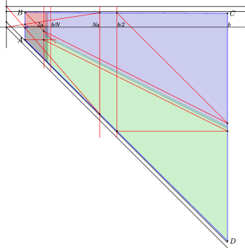
Figure 6. The open set $W_{1}$. The red lines show how to find the colored regions $P^{\prime}_{1},P^{\prime}_{2},P_{2},P_{1}$.

Proposition 7.2.

The open set $W_{1}\subset\operatorname{\rm{Aff}}(1,\mathbb{R})$ satisfies the covering condition with respect to the families $\{F_{1},F_{2},G_{j,1},G_{j,2}\}$ for $j\in\{1,2,3\}$. More precisely, there are polygons $P_{1},P_{2},P_{1}^{\prime},P_{2}^{\prime}\subset\mathbb{R}\times\mathbb{R}^{*}$ covering $\overline{W_{1}}$ such that for each $j\in\{1,2,3\}$,

(7.2) $$P_{1}\cup P_{2}\cup P_{1}^{\prime}\cup P_{2}^{\prime}\subset\bigcup_{i=1,2}F_{i}^{-1}(W_{1})\cup G_{j,i}^{-1}(W_{1}).$$

Proof.

We prove that for any $j\in\{1,2,3\}$ and $i\in\{1,2\}$,

(7.3) $$F_{i}(P_{i}^{\prime})\cup G_{j,i}(P_{i})\subset W_{1}.$$

Clearly, (7.3) implies (7.2). As illustrated in the Figure 6, $P_{i}$ and $P_{i}^{\prime}$ are all compact convex polygons for $i=1,2$ so we will define them with their vertices. We will use the notation $\overline{\operatorname{ch}}({\bf a},{\bf b},{\bf c},{\bf d})$ to describe the closed convex hull of ${\bf a},{\bf b},{\bf c},{\bf d}\subset\mathbb{R}\times\mathbb{R}^{*}$. For $i=1,2$ we shall describe coordinates of points ${\bf a}_{i},{\bf b}_{i},{\bf c}_{i},{\bf d}_{i}$ and ${\bf a}_{i}^{\prime},{\bf b}_{i}^{\prime},{\bf c}_{i}^{\prime},{\bf d}_{i}^{\prime}$ to define $P_{i}:=\overline{\operatorname{ch}}({\bf a}_{i},{\bf b}_{i},{\bf c}_{i},{\bf d}_{i})$ and $P_{i}^{\prime}:=\overline{\operatorname{ch}}({\bf a}_{i}^{\prime},{\bf b}_{i}^{\prime},{\bf c}_{i}^{\prime},{\bf d}_{i}^{\prime})$. Let $\gamma>0$ be sufficiently smaller than $\delta$ and define

$${\bf a}_{1}:=(a,\dfrac{2}{N-1}-a+\dfrac{\delta}{2}), {\bf b}_{1}:=\left(a,\dfrac{(N-4)}{N(N-1)}\right),$$

$${\bf c}_{1}:=\left(\dfrac{b}{N}-\gamma,\dfrac{(N-4)}{N(N-1)}\right), {\bf d}_{1}:=(\dfrac{b}{N}-\gamma,\dfrac{2}{N-1}+\dfrac{\delta}{2}-\dfrac{b}{N}+\gamma),$$

$${\bf a}_{2}:=\left(a,\dfrac{-(N-4)}{N(N-1)}\right), {\bf b}_{2}:=\left(a,\dfrac{N-3}{N-1}-\dfrac{\delta}{2}\right),$$

$${\bf c}_{2}:=\left(\dfrac{b}{N}-\gamma,\dfrac{N-3}{N-1}-\dfrac{\delta}{2}\right), {\bf d}_{2}:=\left(\dfrac{b}{N}-\gamma,\dfrac{-(N-4)}{N(N-1)}\right),$$

$${\bf a}_{1}^{\prime}:=\left(2a+\gamma,\dfrac{2}{N-1}-a+2\delta-\dfrac{\gamma}{2}\right), {\bf b}_{1}^{\prime}:=\left(2a+\gamma,\dfrac{N-3}{N-1}-\delta-\dfrac{\delta(a+\gamma)}{b-a}\right),$$

$${\bf c}_{1}^{\prime}:=\left(b,\dfrac{N-3}{N-1}-2\delta\right), {\bf d}_{1}^{\prime}:=\left(b,\dfrac{2}{N-1}-\dfrac{b}{2}+2\delta\right),$$

$${\bf c}_{2}^{\prime}:=\left(b,\dfrac{N-3}{N-1}-2\delta-\dfrac{b}{2}\right), {\bf d}_{2}^{\prime}:=\left(b,\dfrac{2}{N-1}-b+2\delta\right),$$

$${\bf a}_{2}^{\prime}:=\left(2a+\gamma,\dfrac{2}{N-1}-2a-\gamma+\delta+\dfrac{\delta(a+\gamma)}{b-a}\right),$$

$${\bf b}_{2}^{\prime}:=\left(2a+\gamma,\dfrac{N-3}{N-1}-2\delta-a-\dfrac{\gamma}{2}\right).$$

Given a polygon $P$ and a convex open set $Q$, to show that $\overline{P}\subset Q$ it suffices to prove that the vertices of $P$ lie inside the $Q$. Therefore, observing that $F_{i},G_{i,j}$ are all affine maps from $\mathbb{R}\times\mathbb{R}^{*}$ to $\mathbb{R}^{2}$, the relation (7.3) satisfies because by the definitions above for each $j\in\{1,2,3\}$ we have

$$F_{i}({\bf a}_{i}^{\prime}),F_{i}({\bf b}_{i}^{\prime}) ,F_{i}({\bf c}_{i}^{\prime}),F_{i}({\bf d}_{i}^{\prime})\subset W_{1},$$

$$G_{j,i}({\bf a}_{i}),G_{j,i}({\bf b}_{i}) ,G_{j,i}({\bf c}_{i}),G_{j,i}({\bf d}_{i})\subset W_{1},$$

for $i=1,2$. Note that $W_{1}$ is surrounded by 4 lines. We can describe $W_{1}$ by

$$W_{1}=\left\{(s,t):a<s<b,\;\;\dfrac{2}{N-1}-s+\delta+\dfrac{\delta(s-a)}{b-a}<t<\dfrac{N-3}{N-1}-\delta-\dfrac{\delta(s-a)}{b-a}\right\}.$$

This implies that $\overline{W_{1}}\subset P_{1}\cup P_{2}\cup P_{1}^{\prime}\cup P_{2}^{\prime}$. ∎

Remark 7.3.

Note that in (7.3) contracting maps $F_{i}$ are acting on the regions $P_{i}^{\prime}$, while expanding maps $G_{1,i},G_{2,i},G_{3,i}$ are acting on the regions $P_{i}$ for $i=1,2$. An important property of these regions is that any vertical line intersecting $\overline{W}_{1}$ either intersects $P_{1}\cup P_{2}$ or $P_{1}^{\prime}\cup P_{2}^{\prime}$. Thus, (7.3) implies that we can map all points on a vertical segment inside $\overline{W_{1}}$ into $W_{1}$ via only expanding maps or by only contracting maps. Indeed, all points on such a vertical segment returns back into $W_{1}$ by either the contracting map $F_{i}$ or each of the expanding maps $G_{1,i},G_{2,i},G_{3,i}$, for some $i=1,2$. This observation will play a crucial role in our construction of Cantor sets in higher dimensions.

It follows from Lemma 3.3 that for a relatively open compact set and a finite family of operators the covering condition (3.1) is equivalent to strong covering (3.2). Moreover, the strong covering (3.2) with respect to a finite family is stable under small perturbations (see Lemma 3.4). Hence, by Proposition 7.2, $W_{1}\subset\operatorname{\rm{Aff}}(1,\mathbb{R})$ satisfies strong covering condition with respect to the families of affine maps $\{f_{1},f_{2},g_{j,1}^{-1},g_{j,2}^{-1}\}$ for $j\in\{1,2,3\}$ when $\tau>0$ is small enough. Action of renormalizaion operators $\mathcal{R}_{1}^{*}$ on $\operatorname{\rm{Aff}}(1,\mathbb{R})\cong\mathbb{R}\times\mathbb{R}^{*}$ for the pair $(K_{1},K_{1}^{\prime})$ consists of two contracting maps $f_{1},f_{2}$ which are the generators of $K_{1}^{\prime}$ and six expanding maps $g_{1,1}^{-1},g_{1,2}^{-1},g_{2,1}^{-1},g_{2,2}^{-1},g_{3,1}^{-1},g_{3,2}^{-1}$ obtaining from $K_{1}$. Consider the partition of expanding renormalization operators of the pair $(K_{1},K_{1}^{\prime})$ into two families $\mathcal{A}_{i}:=\{g_{1,i}^{-1},g_{2,i}^{-1},g_{3,i}^{-1}\}$ for $i=1,2$. Consequently, fro sufficiently small enough $\tau$ we have the following.

Corollary 7.4.

$W_{1}$ has expanding $3$-cover with respect to the pair $(K_{1},K_{1}^{\prime})$. Indeed, any ${\bf x}\in\overline{W_{1}}$ returns back into $W_{1}$ by the contracting operator $F_{i}$ when ${\bf x}\in P_{i}^{\prime}$ or by each of the expanding operators in the family $\mathcal{A}_{i}$ whenever ${\bf x}\in P_{i}$, for $i\in\{1,2\}$.

7.2. Cantor sets in $\mathbb{R}^{d}$ with expanding $3^{d}$-cover on $\operatorname{\rm{Aff}}_{\mathrm{Id}}(d,\mathbb{R})$

It is a simple observation that if $K$ is a regular Cantor set in $\mathbb{F}$ generated by an IFS with full shift symbolic type consisting of $n$ contracting maps $f_{1},f_{2},\dots,f_{n}$, then $K^{d}:=K\times K\times\cdots\times K$ is a regular Cantor set in $\mathbb{F}^{d}$ generated by an IFS consisting of $n^{d}$ maps $f_{i_{1}}\times f_{i_{2}}\times\cdots\times f_{i_{d}}$. In the case that $K$ is an affine Cantor set, the map $f_{i_{1}}\times f_{i_{2}}\times\cdots\times f_{i_{d}}:\mathbb{F}^{d}\to\mathbb{F}^{d}$ is an affine map of the form $[x\mapsto Ax+v]$ where $A\in\operatorname{\rm{GL}}(d,\mathbb{F}),v\in\mathbb{F}^{d}$. Hence, $K^{d}$ is an affine Cantor set generated by an IFS consisting of $n^{d}$ affine maps with full shift symbolic type. Furthermore, $\operatorname{dim_{HD}}(K^{d})=d\cdot\operatorname{dim_{HD}}(K)$ (see [27], [9]).

Figure 7. Cantor sets $K_{1}^{d},K_{1}^{\prime d}$ in dimension $d=2$, first step approximation.

Each of the affine generators of the affine Cantor sets $K_{1}^{d},{K^{\prime}_{1}}^{d}$ is equal to composition of a homothety and a translation which is like $[x\mapsto s\cdot x+b]\subset\operatorname{\rm{Aff}}_{\mathrm{Id}}(d,\mathbb{R})$ (see Lemma C for the definition of $\operatorname{\rm{Aff}}_{\mathrm{Id}}(d,\mathbb{R})$). Because the generators $f_{i}$ of $K_{1}^{\prime}$ have same contraction rate $1/(2+\tau)$ which implies that the generators of ${K^{\prime}_{1}}^{d}$ are members of $\operatorname{\rm{Aff}}_{\mathrm{Id}}(d,\mathbb{R})$. Similarly, the generators of $K_{1}^{d}$ belong to $\operatorname{\rm{Aff}}_{\mathrm{Id}}(d,\mathbb{R})$. Thus, the renormalization operators of the pair $(K_{1}^{d},K_{1}^{\prime d})$ belong to $\operatorname{\rm{Aff}}_{\mathrm{Id}}(d,\mathbb{R})$. So, we can study their action on this subgroup.

Denote $W_{d}\subset\operatorname{\rm{Aff}}_{\mathrm{Id}}(d,\mathbb{R})$ as the fiber product of $d$ copies of $W_{1}$ over the base $\mathbb{R}^{*}$ (See Proposition 7.2). More precisely,

$$W_{d}:=\left\{(s,t_{1},t_{2},\dots,t_{d}):(s,t_{i})\in W_{1},\;\;\forall i=1,2,\dots,d\right\}\subset\mathbb{R}^{d}\rtimes\mathbb{R}^{*}\cong\operatorname{\rm{Aff}}_{\mathrm{Id}}(d,\mathbb{R}).$$

Lemma 7.5.

$W_{d}$ has expanding $3^{d}$-cover with respect to the family of renormalization operators of the pair $(K_{1}^{d},K_{1}^{\prime d})$. Moreover, there exists $\varepsilon_{1},\varepsilon_{2}>0$ such that for any $(w,u)\in B_{\varepsilon_{2}}(W_{d})\times\overline{B_{\varepsilon_{1}}(\mathrm{Id})}\subset\operatorname{\rm{Aff}}_{\mathrm{Id}}(d,\mathbb{R})\times\operatorname{\rm{SL}}(d,\mathbb{R})$ either there exists a contracting operator or at least $3^{d}$ expanding operators that maps $(w,u)$ to $(w^{\prime},u)\in(W_{d})_{(\varepsilon_{2})}\times\overline{B_{\varepsilon_{1}}(\mathrm{Id})}$.

Here, by $B_{\varepsilon_{1}}(\mathrm{Id})$ we mean the $\varepsilon_{1}$ neighborhood of $\mathrm{Id}\in\operatorname{\rm{SL}}(d,\mathbb{R})$. Also, $B_{\delta}(W_{d})$ and $(W_{d})_{(\delta)}$ are $\delta$-neighborhood and $\delta$-interior of $W_{d}$ in $\operatorname{\rm{Aff}}_{\mathrm{Id}}(d,\mathbb{R})$ which should not be confused with the ambient space $\operatorname{\rm{Aff}}(d,\mathbb{R})\supset W_{d}$.

Proof.

Let $w=(s,t_{1},\dots,t_{d})\in\overline{W_{d}}$. For each $j=1,2,\dots,d$ there is a renormalization operator $\Psi_{j}$ of the pair $(K_{1},K_{1}^{\prime})$ that maps each $(s,t_{j})$ to $(s_{j},t_{j}^{\prime})\in W_{1}$. Denote the vertical line $L_{s}$ inside $\overline{W_{1}}$ as

$$L_{s}:=\{(s,t):(s,t)\in\overline{W_{1}}\}\subset\overline{W_{1}}$$

By Remark 7.3, we have either $L_{s}\subset P^{\prime}_{1}\cup P^{\prime}_{2}$ or $L_{s}\subset P_{1}\cup P_{2}$. Subsequently, $\Psi_{j}$’s are either all contracting operators or all expanding operators. When $L_{s}\subset P^{\prime}_{1}\cup P^{\prime}_{2}$, $\hat{\Psi}:=\Psi_{1}\times\Psi_{2}\times\cdots\times\Psi_{d}\in\operatorname{\rm{Aff}}_{\mathrm{Id}}(d,\mathbb{R})$ will be a contracting renormalization operator of the pair $(K_{1}^{d},K_{1}^{\prime d})$ which maps $w$ into $W_{d}$. If $L_{s}\subset P_{1}\cup P_{2}$, then by Corollary 7.4 we conclude that there are least three options for each of $\Psi_{j}$, $j=1,\dots,d$. Therefore, there are at least $3^{d}$ expanding renormalization operators of the form $\hat{\Psi}=\Psi_{1}\times\Psi_{2}\times\cdots\times\Psi_{d}\in\operatorname{\rm{Aff}}_{\mathrm{Id}}(d,\mathbb{R})$ which map $w$ into $W_{d}$. This implies that $W_{d}$ has expanding $3^{d}$-cover with respect to the family of the renormalization operators of the pair $(K_{1}^{d},K_{1}^{\prime d})$. By Corollary 7.4, we can partition the family of expanding renormalization operators of the pair $(K_{1}^{d},K_{1}^{\prime d})$ which consists of $6^{d}$ elements as disjoint union $\bigsqcup_{\alpha\in\{1,2\}^{d}}\mathcal{H}_{\underline{\alpha}}$ of $2^{d}$ sets such that for $\underline{\alpha}=(\alpha_{1},\dots,\alpha_{d})$,

(7.4) $$\mathcal{H}_{\underline{\alpha}}:=\{\Psi_{1}\times\Psi_{2}\times\cdots\times\Psi_{d}~:~\Psi_{j}\in\mathcal{A}_{\alpha_{j}},\;1\leq j\leq d\}.$$

This partitioning is such that any $w\in\overline{W_{d}}$ maps into $W_{d}$ by either a contracting operator or any expanding operator in the set $\mathcal{H}_{\underline{\alpha}}$ for some $\underline{\alpha}\in\{1,2\}^{d}$. Lemma 3.3 implies that there is $\delta>0$ such that any $w\in B_{\delta}(W_{d})\subset\operatorname{\rm{Aff}}_{\mathrm{Id}}(d,\mathbb{R})$ maps to $(W_{d})_{(\delta)}$ via either a contracting operator or any expanding one from the set $\mathcal{H}_{\underline{\alpha}}$ for some $\underline{\alpha}\in\{1,2\}^{d}$. Corollary 5.5 helps us to study the action of renormalization operators of the pair $(K_{1}^{d},K_{1}^{\prime d})$ on $\overline{W_{d}}\times\overline{B_{\varepsilon}(\mathrm{Id})}$. Let $(w,u)\in B_{\delta}({W_{d}})\times\overline{B_{\varepsilon}(\mathrm{Id})}$. In the case that $w$ maps to $(W_{d})_{(\delta)}$ by an expanding operator $\Psi\in\mathcal{H}_{\underline{\alpha}}$ for some $\underline{\alpha}\in\{1,2\}^{d}$, because $\Psi\in\operatorname{\rm{Aff}}_{\mathrm{Id}}(d,\mathbb{R})$ and the family of expanding operators act on $\operatorname{\rm{Aff}}(d,\mathbb{R})$ as the product action on $\mathbb{R}^{d}\times(\mathbb{R}^{*}\times\operatorname{\rm{SL}}^{\star}(d,\mathbb{R}))$ then the image of $(w,u)$ is $(\Psi(w),u)\in(W_{d})_{(\delta)}\times\overline{B_{\varepsilon}(\mathrm{Id})}$. In the other case, when $w\in B_{\delta}({W_{d}})$ is mapped into $(W_{d})_{(\delta)}$ by a contracting operator $\Psi$, then the image of $(w,u)$ can be written as $(w^{\prime}_{u},u)$. Note that $w^{\prime}_{\mathrm{Id}}=\Psi(w)\in(W_{d})_{(\delta)}$. But for $u\neq\mathrm{Id}$, $w^{\prime}_{u}$ may differ from $\Psi(w)$, since the action of contracting operators on $\operatorname{\rm{Aff}}(d,\mathbb{R})$ is semidirect product of its action on $\mathbb{R}^{d}$ and $\operatorname{\rm{GL}}(d,\mathbb{R})$. However, $w^{\prime}_{u}$ varies continuously with respect to $u\in\operatorname{\rm{SL}}(d,\mathbb{R})$. Therefore, there exists $\varepsilon_{1}>0$ such that for any $u\in\overline{B_{\varepsilon_{1}}(\mathrm{Id})}\subset\operatorname{\rm{SL}}(d,\mathbb{R})$, $w^{\prime}_{u}\in(W_{d})_{(\delta/2)}$. It suffices to denote $\varepsilon_{2}:=\delta/2$ to yield the result. ∎

Remark 7.6.

Since $W_{d}\subset\mathbb{R}^{d}\times\mathbb{R}^{*}$ is a bounded set, a point cannot remain in $W_{d}$ solely by the action of contracting operators, nor solely by the action of expanding ones. In particular, there exists $T>0$ such that for any $w\in\overline{W_{d}}$ and any sequence $\Psi_{1},\Psi_{2},\dots,\Psi_{T}$ of the operators of the pair $(K_{1}^{d},{K_{1}^{\prime}}^{d})$ such that

$$\Psi_{j}\circ\Psi_{j-1}\circ\cdots\circ\Psi_{1}(w)\in W_{d}$$

for all $1\leq j\leq T$, then there are both expanding and contracting operators among $\Psi_{1},\dots,\Psi_{T}$.

7.3. Examples of stable intersection in any dimension

We are ready to construct a pair of bunched Cantor sets $(K_{d},K_{d}^{\prime})$ in $\mathbb{R}^{d}$ satisfying the covering criterion.

Theorem 7.7.

There exists a pair $(K_{d},K^{\prime}_{d})$ of bunched affine Cantor sets with full shift symbolic type in $\mathbb{R}^{d}$ arbitrarily close to the pair $(K_{1}^{d},K_{1}^{\prime d})$ and an open relatively compact set $\mathcal{U}\subset\operatorname{\rm{SL}}(d,\mathbb{R})$ such that $\mathcal{W}:=W_{d}\times\mathcal{U}\subset\operatorname{\rm{Aff}}(d,\mathbb{R})$ satisfies the strong covering condition with respect to the action of a finite family of renormalization operators of the pair $(K_{d},K^{\prime}_{d})$ on the group $\operatorname{\rm{Aff}}(d,\mathbb{R})$.

Proof of Theorem 7.7.

Let $\varepsilon<\varepsilon_{1}$ be a positive number where $\varepsilon_{1}$ is from Lemma 7.5 and $\delta>0$ be a small constant which will be determined later. According to Lemma 3.7 there exists an open relatively compact set $\mathcal{U}\subset B_{\varepsilon}(\mathrm{Id})\subset\operatorname{\rm{SL}}(d,\mathbb{R})$ and $d^{2}$ matrices $M_{1},\dots,M_{d^{2}}\in B_{\delta}(\mathrm{Id})\subset\operatorname{\rm{SL}}(d,\mathbb{R})$ such that $\mathcal{U}$ satisfies the (strong) covering condition with respect to action of the family $\{M_{1}^{-1},\dots,M_{d^{2}}^{-1}\}$ on $\operatorname{\rm{SL}}(d,\mathbb{R})$.

Consider the families of expanding renormalization operators $\{\mathcal{H}_{\underline{\alpha}}\}_{\underline{\alpha}\in\{1,2\}^{d}}$ of the pair $(K_{1}^{d},K_{1}^{\prime d})$ defined in (7.4). These are inverses of the generators of $K_{1}^{d}$ as has been shown in §5.4. Thus, their $\operatorname{\rm{SL}}$ parts are all $\mathrm{Id}\in\operatorname{\rm{SL}}(d,\mathbb{R})$. Now we perturb the affine generators of the Cantor set $K_{1}^{d}$ to obtain the Cantor set $K_{d}$. This perturbation is such that for each $\underline{\alpha}\in\{1,2\}^{d}$ the $\operatorname{\rm{SL}}$ part of $d^{2}$ generators among the generators corresponded to operators in the family $\mathcal{H}_{\underline{\alpha}}$ be equal to $\{M_{1},M_{2},\dots,M_{d^{2}}\}$. This perturbation can be done because $3^{d}>d^{2}$ and implies that for each $\underline{\alpha}\in\{1,2\}^{d}$ there are $d^{2}$ operators in $\mathcal{H}_{\underline{\alpha}}$ with $\operatorname{\rm{SL}}$ component equal to $M_{1}^{-1},M_{2}^{-1},\dots,M_{d^{2}}^{-1}$. It is important to observe that we do not change determinant or the translation component of the affine generators. The difference of the affine generators of $K_{d}$ and $K_{1}^{d}$ is just in their $\operatorname{\rm{SL}}$ component. Note that $K_{1}^{d}$ and $K_{1}^{\prime d}$ are both conformal Cantor sets. So, their sufficiently small perturbations will be bunched Cantor sets.

Figure 8. Cantor set $K_{d}$ for $d=2$ is illustrated in first step approximation.

Let $K_{d}^{\prime}:=K_{1}^{\prime d}$. The contracting operators of the pair $(K_{1}^{d},K_{1}^{\prime d})$ coincides with the ones of $(K_{d},K_{d}^{\prime})$, since they are the generators of $K_{1}^{\prime d}=K_{d}^{\prime}$. The expanding operators of the pairs $(K_{d},K_{d}^{\prime})$ and $(K_{1}^{d},K_{1}^{\prime d})$ belong to $(\mathbb{R}^{d}\times\mathbb{R}^{*})\times\operatorname{\rm{SL}}(d,\mathbb{R})$ which differ only on their $\operatorname{\rm{SL}}$ part. By (5.30), small changes on $\operatorname{\rm{SL}}$ part of expanding operators affect small changes on their action on the subgroup $\operatorname{\rm{Aff}}_{\mathrm{Id}}(d,\mathbb{R})\cong\mathbb{R}^{d}\times\mathbb{R}^{*}$. So, for small enough $\delta>0$ the action of expanding operators of the pairs $(K_{d},K^{\prime}_{d})$ and $(K_{1}^{d},{K^{\prime}_{1}}^{d})$ on $\operatorname{\rm{Aff}}_{\mathrm{Id}}(d,\mathbb{R})$ are $\varepsilon_{3}$-close where $\varepsilon_{3}:=\varepsilon_{2}/2$ and $\varepsilon_{2}$ is obtained from Lemma 7.5 for the pair $(K_{1}^{d},{K^{\prime}_{1}}^{d})$.

We claim that any $(w,u)\in\overline{W_{d}}\times\overline{\mathcal{U}}\subset B_{\varepsilon_{2}}(W_{d})\times\overline{B_{\varepsilon}(\mathrm{Id})}$ maps to $(W_{d})_{(\varepsilon_{3})}\times\mathcal{U}$ via some renormalization operator of the pair $(K_{d},K^{\prime}_{d})$. According to Lemma 7.5, there is either a contracting operator of the pair $(K_{1}^{d},K_{1}^{\prime d})$ that maps $(w,u)$ to some $(w^{\prime}_{u},u)\in(W_{d})_{(\varepsilon_{2})}\times\overline{\mathcal{U}}$ or an index $\underline{\alpha}\in\{1,2\}^{d}$ such that maps $(w,u)$ to $(w^{\prime},u)\in(W_{d})_{(\varepsilon_{2})}\times\overline{\mathcal{U}}$ via each of expanding operators of the pair $(K_{1}^{d},K_{1}^{\prime d})$ in $\mathcal{H}_{\underline{\alpha}}$. In the first case, since the contracting operators of the pairs $(K_{1}^{d},K_{1}^{\prime d})$ and $(K_{d},K_{d}^{\prime})$ coincide, one can map $(w,u)$ to some $(w^{\prime}_{u},u)\in(W_{d})_{(\varepsilon_{2})}\times\overline{\mathcal{U}}$ by operators of $(K_{d},K^{\prime}_{d})$. By Remark 7.6, after a finite number of iteration of contracting operators we reach to some pair $(w^{*}_{u},u)\in(W_{d})_{(\varepsilon_{2})}\times\overline{\mathcal{U}}$ such that we are able to map $w^{*}_{u}$ into $(W_{d})_{(\varepsilon_{3})}\supset(W_{d})_{(\varepsilon_{2})}$ by an expanding operator of the pair $(K_{1}^{d},{K_{1}^{\prime}}^{d})$. Thus, it only remains to resolve the second case. Since $\mathcal{U}$ satisfies covering condition with respect to the set $\{M_{1}^{-1},\dots,M_{d^{2}}^{-1}\}$, there is $1\leq j\leq d^{2}$ such that $M_{j}^{-1}u=u^{\prime}\in\mathcal{U}$. Thus, the expanding operator from the set $\mathcal{H}_{\underline{\alpha}}$ which is perturbed to have the $\operatorname{\rm{SL}}$ part equal to $M_{j}^{-1}$ maps $(w,u)$ to $(w^{\prime\prime},u^{\prime})$ where $w^{\prime\prime}$ is $\varepsilon_{3}$-close to $w^{\prime}$. Therefore, $(w^{\prime\prime},u^{\prime})\in(W_{d})_{(\varepsilon_{3})}\times\mathcal{U}$. This implies that $\mathcal{W}$ satisfies covering with respect to the finite family of renormalization operators with lengths of words less than $T$. The strong covering is concluded via Lemma 3.3. ∎

Proof of Theorem A.

According to Lemma 3.5, since $\mathcal{W}$ satisfies strong covering with respect to a finite subfamily of renormalization operators of the pair $(K_{d},K^{\prime}_{d})$, there exists a relatively compact $\mathcal{W}^{\prime}\supset\mathcal{W}$ that satisfies the strong covering condition with respect to the (finite) generating family $\mathcal{R}_{1}^{*}$ of renormalization operators of the pair $(K_{d},K_{d}^{\prime})$. Then, since $\mathrm{Id}\in\operatorname{\rm{Aff}}(d,\mathbb{R})$ lies in $\mathcal{W}$, stable intersection of $K_{d}$ and $K_{d}^{\prime}$ follows from Theorems 6.4 and 6.6.

To estimate the dimension of $K_{d}$, we use the system of covering $\{G({\underline{a}})\}_{{\underline{a}}\in X_{n}}$, where $X_{n}\subset\Sigma^{\rm fin}$ denotes the set of all elements of $\Sigma^{\rm fin}$ with length $n$. In particular, for each $n\in\mathbb{N}$, $K_{d}\subset\bigcup_{{\underline{a}}\in X_{n}}G({\underline{a}})$. Note that for all $a\in\mathfrak{A}$, $G(a)$ is contained in the unit square $B$ and $G({\underline{a}}):=f_{{\underline{a}}}(G(a_{n}))$ for each ${\underline{a}}\in X_{n}$. Recall that the construction of $K_{1}$ in §7.1 depends on two parameters $\tau$ and $N$. Now, let $\tau^{\prime}<\tau$ be positive. One can take $\delta>0$ in the proof of Theorem 7.7 in the construction of $K_{d}$ such that for any affine generator $f_{(a,b)}$ of $K_{d}$ we have that $\|Df_{(a,b)}\|_{\it op}\leq(N+\tau^{\prime})^{-1}$. Thus, $\operatorname{\rm{diam}}(G({\underline{a}}))\leq(N+\tau^{\prime})^{-n}$ for any ${\underline{a}}\in X_{n}$ and $n\in\mathbb{N}$. Therefore,

$$\sum_{{\underline{a}}\in X_{n}}\operatorname{\rm{diam}}(G({\underline{a}}))^{s}\leq 6^{nd}\cdot(N+\tau^{\prime})^{-sn}=(6^{d}/(N+\tau^{\prime})^{s})^{n}$$

tends to zero as $n\to\infty$ for any $s>{d\cdot\ln 6}/{\ln(N+\tau^{\prime})}$. This implies that

$$\operatorname{dim_{HD}}(K_{d})\leq\dfrac{d\cdot\ln 6}{\ln(N+\tau^{\prime})}.$$

In particular, given $\varepsilon>0$, if $N$ is taken large enough, then $\operatorname{dim_{HD}}(K_{d})<\varepsilon$. ∎

7.4. Affine bunched holomorphic Cantor sets: proof of Theorem B

To construct a pair of bunched holomorphic Cantor sets in $\mathbb{C}^{d}\cong\mathbb{R}^{2d}$ with an open relatively compact set satisfying the strong covering condition we follow the same argument of previous sections with a small change in the last steps. From Lemma C.1 we have that $\operatorname{\rm{Aff}}(d,\mathbb{C})\cong\mathbb{R}^{2d}\rtimes\left(\mathbb{R}^{*}\times\mathbb{T}^{1}\times\operatorname{\rm{SL}}^{*}(d,\mathbb{C})\right)$ where $\mathbb{T}^{1}$ is the one-dimensional torus. In addition, we have $\mathbb{R}^{2d}\rtimes\mathbb{R}^{*}$ is isomorphic to a subgroup of $\operatorname{\rm{Aff}}_{\mathrm{Id}}(d,\mathbb{C})$ under the injection map $(v,a)\hookrightarrow(v,a,0,\mathrm{Id})$. Therefore, renormalization operators of the pair $(K_{1}^{2d},K_{1}^{\prime 2d})$ are in the subgroup $\mathbb{R}^{2d}\rtimes\mathbb{R}^{*}$ of $\operatorname{\rm{Aff}}(d,\mathbb{C})$ and we have the following analog of the Lemma 7.5 with the same proof.

Lemma 7.8.

$W_{2d}$ has expanding $3^{d}$-cover with respect to renormalization operators of the pair $(K_{1}^{2d},K_{1}^{\prime 2d})$. Moreover, there exists $\varepsilon_{1}.\varepsilon_{2}>0$ such that if $B_{\varepsilon_{1}}(\mathrm{Id})$ and $I_{\varepsilon_{1}}$ are the $\varepsilon_{1}$-neighborhoods of $\mathrm{Id}$ and $0$ in $\operatorname{\rm{SL}}(d,\mathbb{C})$ and $\mathbb{T}^{1}$ respectively, then for any $(w,\theta,u)\in B_{\varepsilon_{2}}(W_{d})\times\overline{I_{\varepsilon_{1}}}\times\overline{B_{\varepsilon_{1}}(\mathrm{Id})}$ either there exists a contracting operator or at least $3^{d}$ expanding operators that maps $(w,\theta,u)$ to $(w^{\prime},\theta,u)\in(W_{d})_{(\varepsilon_{2})}\times\overline{I_{\varepsilon_{1}}}\times\overline{B_{\varepsilon_{1}}(\mathrm{Id})}$.

We have the following theorem, analogous to Theorem 7.7.

Theorem 7.9.

There exists a pair $(K^{\rm Hol}_{d},K^{\prime\rm Hol}_{d})$ of affine holomorphic Cantor sets with full shift symbolic type in $\mathbb{C}^{d}$ arbitrarily close to the pair $(K_{1}^{2d},K_{1}^{\prime 2d})$ and $I\times\mathcal{U}\subset\mathbb{T}^{1}\times\operatorname{\rm{SL}}(d,\mathbb{C})$ which is an open relatively compact set such that $\mathcal{W}:=W_{2d}\times I\times\mathcal{U}$ satisfies strong covering condition with respect to a finite family of renormalization operators of the pair $(K^{\rm Hol}_{d},K^{\prime\rm Hol}_{d})$.

Proof.

The argument is similar to the proof of Theorem 7.7. The only difference is that we use $3^{d}>2d^{2}$ to duplicate the set of matrices $\{M_{1},\dots,M_{d^{2}}\}\subset\operatorname{\rm{SL}}(d,\mathbb{R})$ into the set of matrices

$$\{e^{i\delta}M_{1},e^{-i\delta}M_{1},\dots,e^{i\delta}M_{d^{2}},e^{-i\delta}M_{d^{2}}\}\subset\mathbb{T}^{1}\times\operatorname{\rm{SL}}(d,\mathbb{C})$$

to obtain the covering condition on the set $I\times\mathcal{U}$, where $I:=I_{\varepsilon}$ is the $\varepsilon$-neighborhood of $0$ in $\mathbb{T}^{1}$. ∎

Proof of Theorem B.

The proof is identical to the proof of Theorem A except that here we use Theorem 7.9 and Lemma 7.8 in place of Theorem 7.7 and Lemma 7.5, respectively. The dimension estimate remains unchanged. ∎

Remark 7.10.

Similar arguments can be applied to other Lie groups. In the case of the group $O(d)$, this method yields pairs of stably intersecting Cantor sets within the space of conformal Cantor sets.

Appendix A A convergence lemma

In this appendix we prove a known convergence lemma which allowed us to study infinitesimal geometry of bunched Cantor sets.

Lemma A.1.

Let $\alpha>0$, $V,U\subset\mathbb{R}^{d}$ be bounded open sets that $\overline{V}\subset U$ and $\{g_{m}\}_{m\in\mathbb{N}}$ be a sequence in $\operatorname{\rm{Diff}}^{1+\alpha}_{\rm loc}(\mathbb{R}^{d})$ such that $\operatorname{Dom}(g_{m})\cap\operatorname{Im}(g_{m})\supset U$. If $\sum_{m=1}^{\infty}d_{\mathcal{C}^{1+\alpha}}(g_{m},\mathrm{Id})<\infty$, then the sequence $\{g_{m}\circ g_{m-1}\circ\cdots\circ g_{1}\}_{m\in\mathbb{N}}$ converges in $\operatorname{\rm{Diff}}^{1+\alpha}_{\rm loc}(\mathbb{R}^{d})$ on $\overline{V}$. Moreover, the limit varies $\mathcal{C}^{1}$-continuously with respect to the sequence $\{g_{m}\}_{m\in\mathbb{N}}$ in the following sense. For every $\varepsilon>0$ there exists $\delta>0$ such that if $\{\tilde{g}_{m}\}_{m\in\mathbb{N}}$ be a sequence in $\operatorname{\rm{Diff}}^{1+\alpha}_{\rm loc}(\mathbb{R}^{d})$ with $\sum_{m=1}^{\infty}d_{\mathcal{C}^{1+\alpha}}(g_{m},\tilde{g}_{m})<\delta$ then the resulting limits

$$G:=\lim_{m\rightarrow\infty}g_{m}\circ g_{m-1}\circ\cdots\circ g_{1},\quad\tilde{G}:=\lim_{m\rightarrow\infty}\tilde{g}_{m}\circ\tilde{g}_{m-1}\circ\cdots\circ\tilde{g}_{1}$$

restricted to $\overline{V}$ are $\varepsilon$-close in $\operatorname{\rm{Diff}}^{1}_{\rm loc}(\mathbb{R}^{d})$.

To prove this lemma we shall use the following Hölder estimates from [8, Theorem A.8]. For $U,V$ as in Lemma A.1, $\beta\geq 1$, $\varphi:U\to\mathbb{R}^{d}$ be a $\mathcal{C}^{\beta}$ map and $g,h\in\operatorname{\rm{Diff}}^{\beta}_{\rm loc}(\mathbb{R}^{d})$ whose domain and image both contain $U$, there is a constant $\lambda_{\beta}$ such that the following holds on $\overline{V}$

$$\|\varphi\circ g\|_{\mathcal{C}^{\beta}} \leq\lambda_{\beta}\left(\|\varphi\|_{\mathcal{C}^{1}}\|g\|_{\mathcal{C}^{\beta}}+\|\varphi\|_{\mathcal{C}^{\beta}}\|g\|_{\mathcal{C}^{1}}^{\beta}+\|\varphi\|_{\mathcal{C}^{0}}\right)$$

(A.1) $$\leq\lambda_{\beta}\cdot\|\varphi\|_{\mathcal{C}^{\beta}}\left(\|g\|_{\mathcal{C}^{\beta}}+\|g\|_{\mathcal{C}^{1}}^{\beta}+1\right).$$

Moreover, if $\beta>1$ on $\overline{V}$ we have

$$\|\varphi\circ g-\varphi\circ h\|_{\mathcal{C}^{1}} \leq 2\|\varphi\|_{\mathcal{C}^{1}}\cdot\|g-h\|_{\mathcal{C}^{1}}+\|h\|_{\mathcal{C}^{1}}\cdot\|g-h\|_{\mathcal{C}^{0}}^{\beta-1}\cdot\|\varphi\|_{\mathcal{C}^{\beta}}$$

$$\leq\|\varphi\|_{\mathcal{C}^{\beta}}\cdot\left(2\|g-h\|_{\mathcal{C}^{1}}+\|h\|_{\mathcal{C}^{1}}\cdot\|g-h\|_{\mathcal{C}^{0}}^{\beta-1}\right)$$

(A.2) $$\leq\|\varphi\|_{\mathcal{C}^{\beta}}\cdot\left(2+\|h\|_{\mathcal{C}^{1}}\right)\cdot\left(\|g-h\|_{\mathcal{C}^{1}}+\|g-h\|_{\mathcal{C}^{1}}^{\beta-1}\right).$$

Proof of Lemma A.1.

Denote

$$G_{m}:=g_{m}\circ g_{m-1}\circ\cdots\circ g_{1},\quad\phi_{m}:=g_{m}-\mathrm{Id},\quad\Phi_{m}:=G_{m}-\mathrm{Id}.$$

Note that $\operatorname{Dom}(\phi_{m})=\operatorname{Dom}(g_{m})\supset U$ and $\operatorname{Dom}(\Phi_{m})=\operatorname{Dom}(G_{m})\supset U$. We have

$$\mathrm{Id}+\Phi_{m}=G_{m}=g_{m}\circ G_{m-1}=\mathrm{Id}+\Phi_{m-1}+\phi_{m}\circ(\mathrm{Id}+\Phi_{m-1}),$$

so

(A.3) $$\Phi_{m}-\Phi_{m-1}=\phi_{m}\circ(\mathrm{Id}+\Phi_{m-1}).$$

In addition, the assumption $\sum_{m=1}^{\infty}d_{\mathcal{C}^{1+\alpha}}(g_{m},\mathrm{Id})<\infty$ implies that

(A.4) $$\sum_{m=1}^{\infty}\|\phi_{m}\|_{\mathcal{C}^{1+\alpha}}<\infty.$$

Since $\|\phi_{m}\circ(\mathrm{Id}+\Phi_{m-1})\|_{\mathcal{C}^{0}}\leq\|\phi_{m}\|_{\mathcal{C}^{0}}$, by (A.3) and (A.4) we get that $\{\Phi_{n}\}_{n\geq 1}$ is a Cauchy sequence in $\mathcal{C}^{0}$ topology which yields the $\mathcal{C}^{0}$ convergence.

Let $a_{n}:=\|\phi_{n}\|_{\mathcal{C}^{1+\alpha}}$, $b_{n}:=\|\Phi_{n}\|_{\mathcal{C}^{1}}$ and $c_{n}:=\|\Phi_{n}\|_{\mathcal{C}^{1+\alpha}}$. Then (A.3) and (A) for $\beta=1$ implies that

$$\|\Phi_{m}-\Phi_{m-1}\|_{\mathcal{C}^{1}} =\|\phi_{m}\circ(\mathrm{Id}+\Phi_{m-1})\|_{\mathcal{C}^{1}}$$

$$\leq\lambda_{1}\cdot\|\phi_{m}\|_{\mathcal{C}^{1}}\cdot\left(2\|\mathrm{Id}+\Phi_{m-1}\|_{\mathcal{C}^{1}}+1\right)$$

(A.5) $$\leq 2\lambda_{1}\cdot a_{m}\cdot\left(b_{m-1}+\ell_{0}\right),$$

where $\ell_{0}:=2+\operatorname{\rm{diam}}(U)$. Then, since $b_{m}-b_{m-1}\leq\|\Phi_{m}-\Phi_{m-1}\|_{\mathcal{C}^{1}}$ we have

$$b_{m}+\ell_{0}\leq(b_{m-1}+\ell_{0})(1+2\lambda_{1}\cdot a_{m}).$$

It follows that for $\ell_{1}:=(b_{1}+\ell_{0})/(1+2\lambda_{1}\cdot a_{1})$ and $m\in\mathbb{N}$,

$$b_{m}+\ell_{0} \leq\ell_{1}\cdot\prod_{j=1}^{m}(1+2\lambda_{1}\cdot a_{j}).$$

Since $\sum_{j=1}^{\infty}a_{j}<\infty$, the product $\prod_{j=1}^{\infty}(1+2\lambda_{1}\cdot a_{j})$ converges and the sequence $\{b_{n}\}_{n\in\mathbb{N}}$ is bounded by some $b>0$. In particular, $\|\mathrm{Id}+\Phi_{m-1}\|_{\mathcal{C}^{1}}$ is bounded by $b+\ell_{0}$. To prove $\mathcal{C}^{1+\alpha}$ convergence we proceed with similar calculations. We have

$$\|\Phi_{m}-\Phi_{m-1}\|_{\mathcal{C}^{1+\alpha}} =\|\phi_{m}\circ(\mathrm{Id}+\Phi_{m-1})\|_{\mathcal{C}^{1+\alpha}}$$

$$\leq\lambda_{1+\alpha}\cdot\|\phi_{m}\|_{\mathcal{C}^{1+\alpha}}\cdot\left(\|\mathrm{Id}+\Phi_{m-1}\|_{\mathcal{C}^{1+\alpha}}+\|\mathrm{Id}+\Phi_{m-1}\|_{\mathcal{C}^{1}}^{1+\alpha}+1\right)$$

$$\leq 2\lambda_{1+\alpha}\cdot\|\phi_{m}\|_{\mathcal{C}^{1+\alpha}}\cdot\left(\|\mathrm{Id}+\Phi_{m-1}\|_{\mathcal{C}^{1+\alpha}}+(b+\ell_{0})^{1+\alpha}+1\right)$$

(A.6) $$\leq 2\lambda_{1+\alpha}\cdot a_{m}\cdot\left(c_{m-1}+\ell_{2}\right),$$

where $\ell_{2}:=(b+\ell_{0})^{1+\alpha}+\ell_{0}+1$. Therefore, similar to the argument above there exists $\ell_{3}:=(c_{1}+\ell_{2})/(1+2\lambda_{1+\alpha}\cdot a_{1})$ such that for all $m\in\mathbb{N}$,

$$c_{m}+\ell_{2} \leq\ell_{3}\cdot\prod_{j=1}^{m}(1+2\lambda_{1+\alpha}\cdot a_{j})$$

which implies that the sequence $\{c_{m}\}_{m\in\mathbb{N}}$ is bounded by some $c>0$. So by (A)

(A.7) $$\|\Phi_{m}-\Phi_{m-1}\|_{\mathcal{C}^{1+\alpha}}\leq 2\lambda_{1+\alpha}(c+\ell_{2})\cdot\|\phi_{m}\|_{\mathcal{C}^{1+\alpha}}.$$

Hence, $\{\Phi_{m}\}_{m\in\mathbb{N}}$ is Cauchy by (A.4) and we obtain the $\mathcal{C}^{1+\alpha}$ convergence. The sequence $DG_{m}$ converges to a non-singular matrix $DG$ in the $\mathcal{C}^{1}$ norm which implies that $G$ has a $\mathcal{C}^{1}$ inverse equal to $\lim_{m\rightarrow\infty}G_{m}^{-1}$. Then using [8, Theorem A.9] with similar calculations as above it can be proved that $|DG_{m}^{-1}-DG^{-1}|_{\alpha}$ tends to zero as $m$ goes to infinity which implies that $\lim_{m\rightarrow\infty}G_{m}=G$ is in $\operatorname{\rm{Diff}}^{1+\alpha}_{\rm loc}(\mathbb{R}^{d})$. This completes the proof of first part of the lemma.

To prove the continuity of limit with respect to the sequence $\{g_{m}\}_{m\in\mathbb{N}}$, let

$$\tilde{G}_{m}:=\tilde{g}_{m}\circ\tilde{g}_{m-1}\circ\cdots\circ\tilde{g}_{1},\quad\tilde{\Phi}_{m}:=\tilde{G}_{m}-\mathrm{Id},\quad\tilde{\phi}_{m}:=\tilde{g}_{m}-\mathrm{Id}$$

with $\sum_{m\in\mathbb{N}}d_{\mathcal{C}^{1+\alpha}}(g_{m},\tilde{g}_{m})<\delta$ for some $\delta>0$ to be determined later. By (A)

$$\|\Phi_{m}-\tilde{\Phi}_{m}\|_{\mathcal{C}^{1}}= ~\|(\Phi_{m-1}-\tilde{\Phi}_{m-1})+(\phi_{m}-\tilde{\phi}_{m})\circ(\mathrm{Id}+\tilde{\Phi}_{m-1})$$

$$+\phi_{m}\circ(\mathrm{Id}+\Phi_{m-1})-\phi_{m}\circ(\mathrm{Id}+\tilde{\Phi}_{m-1})\|_{\mathcal{C}^{1}}$$

$$\leq ~\|\Phi_{m-1}-\tilde{\Phi}_{m-1}\|_{\mathcal{C}^{1}}$$

$$+\lambda_{1}\cdot\|\phi_{m}-\tilde{\phi}_{m}\|_{\mathcal{C}^{1}}\cdot\left(2\|\mathrm{Id}+\Phi_{m-1}\|_{\mathcal{C}^{1}}+1\right)$$

$$+\|\phi_{m}\circ(\mathrm{Id}+\Phi_{m-1})-\phi_{m}\circ(\mathrm{Id}+\tilde{\Phi}_{m-1})\|_{\mathcal{C}^{1}}$$

$$\leq ~\|\Phi_{m-1}-\tilde{\Phi}_{m-1}\|_{\mathcal{C}^{1}}+\lambda_{1}\cdot\ell_{4}\cdot\|\phi_{m}-\tilde{\phi}_{m}\|_{\mathcal{C}^{1}}$$

(A.8) $$+\|\phi_{m}\circ(\mathrm{Id}+\Phi_{m-1})-\phi_{m}\circ(\mathrm{Id}+\tilde{\Phi}_{m-1})\|_{\mathcal{C}^{1}},$$

where $\ell_{4}:=1+2(\ell_{0}+b)$. Using the estimate (A) one has

$$\|\phi_{m}\circ (\mathrm{Id}+\Phi_{m-1})-\phi_{m}\circ(\mathrm{Id}+\tilde{\Phi}_{m-1})\|_{\mathcal{C}^{1}}$$

(A.9) $$\leq\|\phi_{m}\|_{\mathcal{C}^{1+\alpha}}\cdot(2+\|\Phi_{m-1}\|_{\mathcal{C}^{1}})\cdot\left(\|\Phi_{m-1}-\tilde{\Phi}_{m-1}\|_{\mathcal{C}^{1}}+\|\Phi_{m-1}-\tilde{\Phi}_{m-1}\|_{\mathcal{C}^{1}}^{\alpha}\right).$$

Let $s_{m}:=\|\Phi_{m}-\tilde{\Phi}_{m}\|_{\mathcal{C}^{1+\alpha}}$ and $t_{m}:=\|\phi_{m}-\tilde{\phi}_{m}\|_{\mathcal{C}^{1+\alpha}}$. By (A) and (A.9) we have

$$s_{m} \leq s_{m-1}+\lambda_{1}\ell_{4}\cdot t_{m}+(2+b)\cdot a_{m}\cdot(s_{m-1}+s_{m-1}^{\alpha})$$

(A.10) $$\leq s_{m-1}(1+\ell_{4}\cdot a_{m})+s_{m-1}^{\alpha}\cdot\ell_{4}\cdot a_{m}+\lambda_{1}\ell_{4}\cdot t_{m},$$

Since $\sum_{m=1}^{\infty}a_{m}<\infty$, there exists $m_{0}\in\mathbb{N}$ such that $\sum_{j\geq m_{0}}a_{j}<(8\ell_{4})^{-1}$. Thus, by $\sum_{m\in\mathbb{N}}t_{m}<\delta$, if $\delta<(4\lambda_{1}\ell_{4})^{-1}$ we have $\sum_{j\geq m_{0}}(2\ell_{4}a_{j}+\lambda_{1}\ell_{4}t_{j})<1/2$. On the other hand, by continuity of finite composition $g_{m_{0}}\circ\cdots\circ g_{1}$ with respect to $g_{1},\dots,g_{m_{0}}$, there is a small $\delta_{0}>0$ such that for $\delta<\delta_{0}$ we have $s_{1},s_{2},\dots,s_{m_{0}}<1/2$. Arguing by induction we show that for $m\geq m_{0}$ one has

$$s_{m}\leq 1-\sum_{j\geq m+1}(2\ell_{4}a_{j}+\lambda_{1}\ell_{4}t_{j}).$$

Since $s_{m-1}<1$, we have $s_{m-1}^{\alpha}<1$. So by (A) we can write

$$s_{m} \leq s_{m-1}+(2\ell_{4}a_{m}+\lambda_{1}\ell_{4}t_{m})$$

$$\leq 1-\sum_{j\geq m}(2\ell_{4}a_{j}+\lambda_{1}\ell_{4}t_{j})+(2\ell_{4}a_{m}+\lambda_{1}\ell_{4}t_{m})$$

$$=1-\sum_{j\geq m+1}(2\ell_{4}a_{j}+\lambda_{1}\ell_{4}t_{j}),$$

and the induction step follows. Thus, $s_{m}<1$ for all $m\in\mathbb{N}$. So by (A) we have

$$s_{m} \leq s_{m-1}(1+\ell_{4}\cdot a_{m})+s_{m-1}^{\alpha}\cdot\ell_{4}\cdot a_{m}+\lambda_{1}\ell_{4}\cdot t_{m}$$

(A.11) $$\leq s_{m-1}+\ell_{5}\cdot u_{m},$$

where $\ell_{5}:=\ell_{4}(1+\lambda_{1})$ and $u_{m}:=2a_{m}+t_{m}$. Thus, for all $m,N\in\mathbb{N}$ we have

$$s_{m+N} \leq s_{m}+\ell_{5}\sum_{j=1}^{N}u_{m+j}$$

(A.12) $$\leq s_{m}+\ell_{5}\sum_{j>m}u_{j}.$$

So, given $\varepsilon>0$ there is a large enough $m_{1}$ such that $\sum_{j\geq m_{1}}a_{j}<\varepsilon(8\ell_{5})^{-1}$, which implies that for $\delta<\varepsilon(4\ell_{5})^{-1}$ and all $N\in\mathbb{N}$, $s_{m_{1}+N}<s_{m_{1}}+\varepsilon/2$. By continuity of the finite composition $g_{m_{1}}\circ\cdots\circ g_{1}$ with respect to $g_{1},\dots,g_{m_{1}}$, there is a small $\delta_{1}>0$ such that for $\delta<\delta_{1}$ we have $s_{m_{1}}<\varepsilon/2$. Therefore, for all $N\in\mathbb{N}$ when $\delta:=\min\{\delta_{0},\delta_{1},\varepsilon(4\ell_{5})^{-1},(4\lambda_{1}\ell_{4})^{-1}\}$ we have $s_{m_{1}+N}<\varepsilon$. Note that $m_{1},m_{0}$ are depended only on the sequence $\{g_{m}\}_{m\in\mathbb{N}}$. This yields the second part of the lemma. ∎

Remark A.2.

Continuity of the limit $G=\lim_{n\to\infty}G_{m}$ also holds in $\mathcal{C}^{1+\alpha^{\prime}}$ topology for any positive $\alpha^{\prime}<\alpha$ rather than $\mathcal{C}^{1}$ topology as stated in Lemma A.1. More generally, same calculations can be done to prove $\mathcal{C}^{\ell}$-convergence of maps $G_{m}$ for any $\ell\geq 1$ provided that $\{g_{m}\}_{m\in\mathbb{N}}$ are maps in $\operatorname{\rm{Diff}}^{\ell}_{\rm loc}(\mathbb{R}^{d})$. Moreover, when $\ell>1$ the limit is continuous in $\mathcal{C}^{\ell^{\prime}}$ topology for any $1\leq\ell^{\prime}<\ell$.

Remark A.3.

If we have $d_{\mathcal{C}^{1+\alpha}}(g_{m},\mathrm{Id})\leq C\cdot\gamma^{m}$ for some positive constants $C$ and $\gamma<1$ then the speed of convergence $G_{m}\rightarrow H$ is about $\gamma^{m}$. In fact there is a constant $C_{1}$ such that $d_{\mathcal{C}^{1+\alpha}}(G_{m},H)\leq C_{1}\cdot\gamma^{m}$.

From the triangle inequality

$$\big{|}d_{\mathcal{C}^{1+\alpha}}(g_{m},\tilde{g}_{m})-d_{\mathcal{C}^{1+\alpha}}(\tilde{g}_{m},\mathrm{Id})\big{|}<d_{\mathcal{C}^{1+\alpha}}(g_{m},\mathrm{Id}),$$

we conclude that whenever $\sum_{m}d_{\mathcal{C}^{1+\alpha}}(g_{m},\mathrm{Id})<\infty$, then $\sum_{m}d_{\mathcal{C}^{1+\alpha}}(\tilde{g}_{m},\mathrm{Id})<\infty$ is equivalent to $\sum_{m}d_{\mathcal{C}^{1+\alpha}}(\tilde{g}_{m},g_{m})<\infty$. Therefore, according to the proof of continuity of the limit $H=\lim_{m\to\infty}G_{m}$ with respect to the sequence $\{g_{m}\}_{m\in\mathbb{N}}$ in Lemma A.1, specifically the relation (A), we have the following continuity lemma which is a variant of the continuity part of Lemma A.1.

Lemma A.4.

Let $C,\epsilon>0$ and $0<\gamma<1$ and $\{g_{m}\}_{m\in\mathbb{N}}$ be a sequence of maps satisfying conditions in Lemma A.1 such that $d_{\mathcal{C}^{1+\alpha}}(g_{m},\mathrm{Id})<C\cdot\gamma^{m}$ for all $m\in\mathbb{N}$. Then there exists $\delta>0$ and an integer $m_{0}>0$ such that for any sequence of maps $\{\tilde{g}_{m}\}_{m=1}^{\infty}$ such that $d_{\mathcal{C}^{1+\alpha}}(\tilde{g}_{m},\mathrm{Id})<C\cdot\gamma^{m}$ for all $m\in\mathbb{N}$, $d_{\mathcal{C}^{1}}(H,\tilde{H})<\epsilon$ if $d_{\mathcal{C}^{1}}(g_{k},\tilde{g}_{k})<\delta$ for $k=1,2,\dots,m_{0}$.

Appendix B Affine estimation

Here we prove the following general linear estimation which is a generalization of [1, Claim 3.9] in arbitrary dimensions, with no conformality assumption.

Lemma B.1.

Let $U\subset\mathbb{R}^{d}$ an open set, $X\subset U$ a set such that it’s convex hull is also contained inside $U$, $p\in X$ a given point, $\phi:U\rightarrow\mathbb{R}^{d}$ be a $\mathcal{C}^{1+\alpha}$ map with $\mathcal{C}^{1+\alpha}$ norm $C_{\phi,X}$ on the domain $X$ and $B\in\operatorname{\rm{Aff}}(d,\mathbb{R})$ be an affine contracting map such that there are constants $C_{B,X}$ and $C_{\phi}$ where

$$C_{B,X}^{-1}\leq\dfrac{\|DB\|_{\it op}}{\operatorname{diam}(X)}\leq C_{B,X},\;\;C_{\phi}:=\sup_{x\in X}\|(D\phi_{x})^{-1}\|_{\it op}.$$

Denote $A_{\phi,p}$ as the affine estimation of $\phi$ which is an affine map with derivative equal to $D\phi_{p}$ and maps $p$ to $\phi(p)$. Then the following holds on the domain $B^{-1}(X)$

$$\|B^{-1}\circ A_{\phi,p}^{-1}\circ\phi\circ B-\mathrm{Id}\|_{\mathcal{C}^{1+\alpha}}<C^{\prime}\cdot\|DB^{-1}\|_{\textit{op}}\cdot\|DB\|_{\textit{op}}\cdot\operatorname{\rm{diam}}(X)^{\alpha},$$

where $C^{\prime}=C_{\phi,X}\cdot(1+2C_{B,X})\cdot C_{\phi}$.

Proof.

Denote $F:=B^{-1}\circ A_{\phi,p}^{-1}\circ\phi\circ B-\mathrm{Id}$. Given an affine map $H\in\operatorname{\rm{Aff}}(d,\mathbb{R})$ and $\psi$ a map on $\mathbb{R}^{d}$, then one has

(B.1) $$H\circ\psi-\mathrm{Id}=DH\circ(\psi-H^{-1}).$$

Taking $H=B^{-1}\circ A_{\phi,p}^{-1}$ and $\psi=\phi\circ B$ in (B.1) implies that

$$F=DB^{-1}\circ DA_{\phi,p}^{-1}\circ(\phi-A_{\phi,p})\circ B.$$

On the other hand, using the Hölder regularity of $\phi$ on domain $X$ we have

(B.2) $$\|\phi-A_{\phi,p}\|_{\mathcal{C}^{0}}\leq C_{\phi,X}\cdot\operatorname{diam}(X)^{1+\alpha},\;\;\|D\phi_{x}-D\phi_{p}\|_{\it op}\leq C_{\phi,X}\cdot\operatorname{diam}(X)^{\alpha}.$$

Then using above relations we have the following estimates on $\mathcal{C}^{1+\alpha}$ norm of $F$.

$$\|F\|_{\mathcal{C}^{0}} \leq\|DB^{-1}\|_{\it op}\cdot\|(D\phi_{p})^{-1}\|_{\it op}\cdot\|\phi-A_{\phi,p}\|_{\mathcal{C}^{0}}$$

$$\leq C_{\phi,X}\cdot C_{B,X}\cdot C_{\phi}\cdot\|DB^{-1}\|_{\it op}\cdot\|DB\|_{\it op}\cdot\operatorname{diam}(X)^{\alpha},$$

$$\|DF\|_{\mathcal{C}^{0}} \leq\|DB^{-1}\|_{\it op}\cdot\|(D\phi_{p})^{-1}\|_{\it op}\cdot\sup_{x\in X}\|D\phi_{x}-D\phi_{p}\|_{\it op}\cdot\|DB\|_{\it op}$$

$$\leq C_{\phi,X}\cdot C_{\phi}\cdot\|DB^{-1}\|_{\it op}\cdot\|DB\|_{\it op}\cdot\operatorname{diam}(X)^{\alpha},$$

$$|DF|_{\alpha} =\sup_{x,y\in B^{-1}(X)}\dfrac{\|DB^{-1}\circ(D\phi_{p})^{-1}\circ(D\phi_{B(x)}-D\phi_{B(y)})\circ DB\|_{\it op}}{|x-y|^{\alpha}}$$

$$\leq C_{\phi,X}\cdot C_{\phi}\cdot C_{B,X}\cdot\|DB^{-1}\|_{\it op}\cdot\|DB\|_{\it op}\cdot\operatorname{diam}(X)^{\alpha}.$$

Thus, since $\|F\|_{\mathcal{C}^{1+\alpha}}\leq\|F\|_{\mathcal{C}^{0}}+\|DF\|_{\mathcal{C}^{0}}+|DF|_{\alpha}$ we conclude the proof. ∎

Appendix C Operations on the space of affine maps

Here, we study the structure of left and right action of $\operatorname{\rm{Aff}}(d,\mathbb{F})$ on itself. Denote

$$\operatorname{\rm{SL}}^{\pm}(d,\mathbb{R}):=\{A\in\operatorname{\rm{SL}}(d,\mathbb{R})~|~\det(A)=\pm 1\}.$$

Let $\operatorname{\rm{SL}}^{\star}(d,\mathbb{F})$ be a notation for $\operatorname{\rm{SL}}(d,\mathbb{F})$ in the cases that $(d,\mathbb{F})=(2k+1,\mathbb{R})$ or $\mathbb{F}=\mathbb{C}$ and for $\operatorname{\rm{SL}}^{\pm}(d,\mathbb{R})$ in the case of $(d,\mathbb{F})=(2k,\mathbb{R})$. Then we have the correspondence $\operatorname{\rm{Aff}}(d,\mathbb{R})\cong\mathbb{R}^{d}\times\mathbb{R}^{*}\times\operatorname{\rm{SL}}^{\star}(d,\mathbb{R})$ via the homeomorphism

$$(v,\lambda,A)\mapsto[x\mapsto\lambda\cdot Ax+v]$$

with the inverse map

$$[x\mapsto Ax+v]\mapsto\left(v,s_{A},s_{A}^{-1}A\right)$$

where $s_{A}:=\frac{\operatorname{det}(A)}{|\operatorname{det}(A)|}\sqrt[d]{|\operatorname{det}(A)|}$. Similarly, $\operatorname{\rm{Aff}}(d,\mathbb{C})\cong\mathbb{C}^{d}\times\mathbb{C}^{*}\times\operatorname{\rm{SL}}^{\star}(d,\mathbb{C})$ via the homeomorphism

$$(v,\lambda e^{i\theta},A)\mapsto[z\mapsto\lambda e^{i\frac{\theta}{d}}\cdot Az+v]$$

where $\lambda>0$ is a real number, with the inverse map

$$[z\mapsto Az+v]\mapsto\left(v,s_{A},s_{A}^{-1}A\right),$$

where $s_{A}:=e^{i\operatorname{arg}(\operatorname{det}(A))}\sqrt[d]{|\operatorname{det}(A)|}$. Let $[x\mapsto Px+w]$ be an element of $\operatorname{\rm{Aff}}(d,\mathbb{F})$. Then for any affine map $[x\mapsto Ax+v]\in\operatorname{\rm{Aff}}(d,\mathbb{F})$ we have

$$[x\mapsto Px+w]\circ[x\mapsto Ax+v]=[x\mapsto PAx+(Pv+w)],$$

$$[x\mapsto Ax+v]\circ[x\mapsto Px+w]=[x\mapsto APx+(v+Aw)].$$

So, we have the following interpretation of the action of the group $\operatorname{\rm{Aff}}(d,\mathbb{F})$ on itself.

Lemma C.1.

The above correspondence is a group homomorphism with the following group operation on $\mathbb{F}^{d}\rtimes(\mathbb{F}^{*}\times\operatorname{\rm{SL}}^{\star}(d,\mathbb{F}))$,

$$(v,a,A)*(w,b,B)=(a\cdot Aw+v,ab,AB).$$

This implies that $\mathbb{F}^{d}\rtimes\mathbb{F}^{*}$ is a subgroup of $\operatorname{\rm{Aff}}(d,\mathbb{F})$ under the injection map $(v,a)\hookrightarrow(v,a,\mathrm{Id})$ with group operation

(C.1) $$(v,a)*(w,b)=(aw+v,ab).$$

We denote the subgroup $\mathbb{F}^{d}\rtimes\mathbb{F}^{*}$ in above definition as $\operatorname{\rm{Aff}}_{\mathrm{Id}}(d,\mathbb{F})$, i.e. subgroup of affine maps that are composition of a homothety and translation.

References

• AM [23] H. Araújo and C. G. Moreira, Stable intersections of conformal Cantor sets, Ergod. Theory Dyn. Syst. 43 (2023), no. 1, 1–49.
• [2] H. Araújo, C. G. Moreira, and A. Zamudio, Stable intersections of regular conformal cantor sets with large hausdorff dimensions, arXiv: 2102.07283.
• Asa [22] M. Asaoka, Stable intersection of Cantor sets in higher dimension and robust homoclinic tangency of the largest codimension, Trans. A. M. S. 375 (2022), no. 2, 873–908.
• BD [96] C. Bonatti and L. J. Díaz, Persistent nonhyperbolic transitive diffeomorphisms, Ann. Math. (2) 143 (1996), no. 2, 357–396.
• Bie [20] S. Biebler, A complex gap lemma, Proc. A. M. S. 148 (2020), no. 1, 351–364.
• Buz [97] G. T. Buzzard, Infinitely many periodic attractors for holomorphic maps of $2$ variables, Ann. Math. (2) 145 (1997), no. 2, 389–417.
• FNR [25] A. Fakhari, M. Nassiri, and H. Rajabzadeh, Stable local dynamics: Expansion, quasi-conformality and ergodicity, Adv. Math. 462 (2025), 110088.
• Hö [76] L. Hörmander, The boundary problems of physical geodesy, Arch. Rational Mech. Anal. 62 (1976), no. 1, 1–52.
• Mat [95] P. Mattila, Geometry of sets and measures in Euclidean spaces, Cambridge Studies in Advanced Mathematics, vol. 44, Cambridge Uni. Press, 1995.
• Mor [96] C. G. Moreira, Stable intersections of Cantor sets and homoclinic bifurcations, Ann. Inst. H. Poincaré C Anal. Non Linéaire 13 (1996), no. 6, 741–781.
• Mor [11] by same author, There are no $C^{1}$-stable intersections of regular Cantor sets, Acta Math. 206 (2011), no. 2, 311–323.
• MS [12] C. G. Moreira and W. L. Silva, On the geometry of horseshoes in higher dimensions, arXiv: 1210.2623 (2012).
• MY [01] C.G Moreira and J. C. Yoccoz, Stable intersections of regular Cantor sets with large Hausdorff dimensions, Ann. Math. (2) 154 (2001), no. 1, 45–96.
• MY [10] C. G. Moreira and J. C. Yoccoz, Tangences homoclines stables pour des ensembles hyperboliques de grande dimension fractale, Ann. Sci. Éc. Norm. Supér. (4) 43 (2010), no. 1, 1–68.
• New [70] S. Newhouse, Nondensity of axiom ${\rm A}({\rm a})$ on $\mathbb{S}^{2}$, Global Analysis (Proc. Sympos. Pure Math., Vol. XIV, Berkeley, Calif., 1968), A. M. S., Providence, R.I., 1970, pp. 191–202.
• New [74] by same author, Diffeomorphisms with infinitely many sinks, Topology 13 (1974), 9–18.
• New [79] by same author, The abundance of wild hyperbolic sets and nonsmooth stable sets for diffeomorphisms, Publ. Math. I. H. É. S. (1979), no. 50, 101–151.
• NP [12] M. Nassiri and E. R. Pujals, Robust transitivity in Hamiltonian dynamics, Ann. Sci. Éc. Norm. Supér. (4) 45 (2012), no. 2, 191–239.
• NPT [83] S. Newhouse, J. Palis, and F. Takens, Bifurcations and stability of families of diffeomorphisms, Publ. Math. I. H. É. S. (1983), no. 57, 5–71.
• [20] M. Nassiri and M. Zareh Bidaki, Cantor sets in higher dimensions II: absence of $\mathcal{C}^{1}$-stable intersection, In preparation.
• Pal [87] J. Palis, Homoclinic orbits, hyperbolic dynamics and dimension of Cantor sets, Contemp. Math. 58, III (1987), 203–216.
• Pal [05] by same author, A global perspective for non-conservative dynamics, Ann. Inst. H. Poincaré C Anal. Non Linéaire 22 (2005), no. 4, 485–507.
• Pou [15] M. Pourbarat, Stable intersection of middle-$\alpha$ Cantor sets, Commun. Contemp. Math. 17 (2015), no. 5, 1550030–19.
• Pou [19] by same author, Stable intersection of affine Cantor sets defined by two expanding maps, J. Differential Equations 266 (2019), no. 4, 2125–2141.
• PT [85] J. Palis and F. Takens, Cycles and measure of bifurcation sets for two-dimensional diffeomorphisms, Invent. Math. 82 (1985), no. 3, 397–422.
• PT [87] by same author, Hyperbolicity and the creation of homoclinic orbits, Ann. Math. (2) 125 (1987), no. 2, 337–374.
• PT [93] by same author, Hyperbolicity and sensitive chaotic dynamics at homoclinic bifurcations, Cambridge Studies in Advanced Mathematics, vol. 35, Cambridge University Press, Cambridge, 1993.
• PV [94] J. Palis and M. Viana, High dimension diffeomorphisms displaying infinitely many periodic attractors, Ann. Math. (2) 140 (1994), no. 1, 207–250.
• PY [09] J. Palis and J. C. Yoccoz, Non-uniformly hyperbolic horseshoes arising from bifurcations of Poincaré heteroclinic cycles, Publ. Math. I. H. É. S. (2009), no. 110, 1–217.
• Sul [88] D. Sullivan, Differentiable structures on fractal like sets, determined by intrinsic scaling functions on dual cantor sets, pp. 101–110, Springer US, 1988.
• Tak [19] Yuki Takahashi, Sums of two homogeneous cantor sets, Trans. A. M. S. 372 (2019), no. 3, 1817–1832.
• Yav [22] Alexia Yavicoli, Thickness and a gap lemma in $\mathbb{R}^{d}$, Int. Math. R. Not. 2023 (2022), no. 19, 16453–16477.