Uncertainty Quantification with the Empirical Neural Tangent Kernel

Abstract

While neural networks have demonstrated impressive performance across various tasks, accurately quantifying uncertainty in their predictions is essential to ensure their trustworthiness and enable widespread adoption in critical systems. Several Bayesian uncertainty quantification (UQ) methods exist that are either cheap or reliable, but not both. We propose a post-hoc, sampling-based uncertainty quantification (UQ) method for overparameterized networks at the end of training. Our approach constructs efficient and meaningful deep ensembles by employing a (stochastic) gradient-descent sampling process on appropriately linearized networks. We demonstrate that our method effectively approximates the posterior of a Gaussian Process using the empirical Neural Tangent Kernel. Through a series of numerical experiments, we show that our method not only outperforms competing approaches in computational efficiency–often reducing costs by multiple factors–but also maintains state-of-the-art performance across a variety of UQ metrics for both regression and classification tasks.

1 Introduction

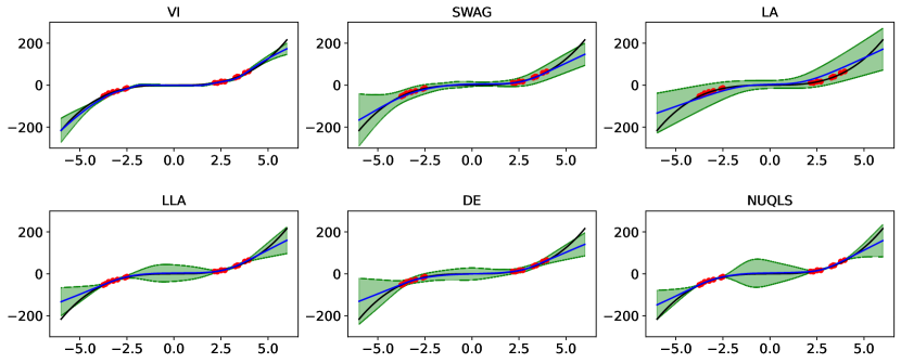
Figure 1: Comparison of various Bayesian UQ methods (see Section 2) on a 1-layer MLP, trained on the data (red) lying on $y=x^{3}$ (black), with Gaussian noise added. The methods’ mean predictors (blue) $\pm 3\sigma$ (green) are shown, where $\sigma^{2}$ is the variance estimated via each method. Clearly, VI, SWAG and LA all perform poorly on this task, while DE performs better, and LLA and NUQLS perform well.

Neural networks (NN) achieve impressive performance on a wide array of tasks, in areas such as speech recognition (Nassif et al., 2019; Abdel-Hamid et al., 2014; Deng et al., 2013), image classification (LeCun et al., 1998; Krizhevsky et al., 2012; He et al., 2016), computer vision (Redmon et al., 2016; Redmon & Farhadi, 2017), and language processing (Vaswani et al., 2017; Ray, 2023; Devlin et al., 2019), often significantly exceeding human performance. While the promising predictive and generative performance of modern NNs is evident, accurately quantifying uncertainty in their predictions remains an important and active research frontier (Abdar et al., 2021). Models are often over-confident in predictions on out-of-distribution (OoD) inputs (Guo et al., 2017), and sensitive to distribution-shift (Ford et al., 2019). By quantifying a model’s uncertainty, we can determine when it fails to provide well-calibrated predictions, indicating the need for additional training (possibly on more diverse data) or even human intervention. This is vital for deploying NNs in critical applications like diagnostic medicine and autonomous machine control (Nemani et al., 2023b).

An array of uncertainty quantification methods for NNs exist, each with benefits and drawbacks. Frequentist statistical methods, such as conformal prediction (Vovk et al., 2005; Papadopoulos et al., 2002; Lei & Wasserman, 2014), create prediction intervals through parameter estimation and probability distributions on the data. While currently considered state-of-the-art, the main drawback is that conformal prediction is data-hungry, requiring a large hold-out set. In contrast, parametric Bayesian methods model the uncertainty in the parameters, providing conditional predictive probabilities for each function output.

Unfortunately, largely due to the curse of dimensionality, existing Bayesian methods are very expensive to compute, and provide poor approximations to the predictive distribution (Folgoc et al., 2021). This results in a suite of methods that require excessive approximations to scale to large problems (Daxberger et al., 2021), often at the cost of theoretical underpinnings, or necessitating modifications to the network itself (He et al., 2020).

Several works (Altieri et al., 2024; Dadalto et al., 2023; Granese et al., 2021) employ the feature-space representations of the network to quantify the uncertainty of test predictions, through kernel densities (Kotelevskii et al., 2022), Gaussian Discriminant analysis (Mukhoti et al., 2023), non-constant mapping functions (Tagasovska & Lopez-Paz, 2019), etc. The interpretation of uncertainty in these works is related to risk of misclassification; these methods generally perform very well at detecting OoD points.While both conformal predictions and the feature-space works just mentioned are important, we limit our scope to Bayesian methods in this paper. Though Bayesian methods can suffer from prior misspecification (Masegosa, 2020) and computational burdens, the predictive and posterior distributions of a model are very natural frameworks for quantifying the uncertainty and spread of possible values of the model.

Gaussian Processes (GPs) (Rasmussen & Williams, 2005) are important tools in Bayesian machine learning (ML) that can directly capture the epistemic (model) uncertainty of predictions, and arise as large-width limits of NNs (Neal, 1996). However, naïve GP training scales cubically in the number of training datapoints, necessitating approximations for modern applications. Neural Tangent Kernels (NTKs) (Jacot et al., 2018) describe the functional evolution of a NN under gradient flow, and naturally arise in the analysis of model quality (Hodgkinson et al., 2023). Due to their deep connection to NNs, these covariance functions are enticing as potential tools for UQ of their corresponding NNs.

Motivated by this, we present a UQ method for a trained, over-parameterized NN model, wherein we approximate the predictive distribution through an ensemble of linearized models, trained using (stochastic) gradient-descent. For certain loss functions, this ensemble samples from the posterior of a GP with an empirical NTK.

Contributions. Our contributions are as follows:

1. We present a Monte-Carlo sampling based UQ method to approximate the predictive distribution of NNs, called Neural Uncertainty Quantification by Linearized Sampling (NUQLS). Our method is lightweight, post-hoc, numerically stable, and embarrassingly parallel.

2. Under certain assumptions, we show that NUQLS converges to the predictive distribution of a GP with an empirical NTK kernel, providing a novel perspective on the connection between NNs, GPs, and the NTK.

3. On various ML problems, we show that NUQLS performs as well as or better than leading UQ methods, is less computationally expensive than deep ensemsble, and scales to large image classification tasks.

Notation.

Throughout the paper, we denote scalars, vectors, and matrices as lower-case, bold lower-case, and bold upper-case letters, e.g., $c$, $\bm{\theta}$ and ${{\mathbf{K}}}$, respectively. For two vectors ${\bf v}\in^{p}$ and ${\bf w}\in^{p}$, their Euclidean inner product is denoted as $\left\langle{\bf v},{\bf w}\right\rangle={\bf v}^{{{\mathchoice{\raisebox{0.0pt}{$\displaystyle\intercal$}}{\raisebox{0.0pt}{$\textstyle\intercal$}}{\raisebox{0.0pt}{$\scriptstyle\intercal$}}{\raisebox{0.0pt}{$\scriptscriptstyle\intercal$}}}}}{\bf w}$. We primarily consider supervised learning, which involves a function ${\bf f}:^{d}\times^{p}\to^{c}$, assumed sufficiently smooth in its parameters $\bm{\theta}\in^{p}$, a training dataset $\mathcal{D}=\{\mathcal{X},\mathcal{Y}\}=\{{\bf x}_{i},{\bf y}_{i}\}_{i=1}^{n}\subset^{d}\times^{c}$, and a loss function $\ell:^{c}\times^{c}\to[0,\infty)$.

The process of training amounts to finding a solution, $\widehat{\bm{\theta}}$, to the optimization problem $\min_{\bm{\theta}}\sum_{i=1}^{n}\ell({\bf f}({\bf x}_{i},\bm{\theta}),{\bf y}_{i})+\mathcal{R}(\bm{\theta})$, where $\mathcal{R}(\bm{\theta})$ is a regulariser. For a kernel function ${{\mathbf{K}}}:^{d}\times^{d}\to^{c\times c}$, we define ${{\mathbf{K}}}_{\mathcal{X},\mathcal{X}}\in^{nc\times nc}$ where the $(i,j)^{\text{th}}$ (block) element is ${{\mathbf{K}}}({\bf x}_{i},{\bf x}_{j})\in^{c\times c}$. Additionally, we define ${{\mathbf{K}}}_{\mathcal{X},{\bf x}}\triangleq\begin{bmatrix}{{\mathbf{K}}}({\bf x}_{1},{\bf x})&\ldots&{{\mathbf{K}}}({\bf x}_{n},{\bf x})\end{bmatrix}^{{{\mathchoice{\raisebox{0.0pt}{$\displaystyle\intercal$}}{\raisebox{0.0pt}{$\textstyle\intercal$}}{\raisebox{0.0pt}{$\scriptstyle\intercal$}}{\raisebox{0.0pt}{$\scriptscriptstyle\intercal$}}}}}\in^{nc\times c}$ with ${{\mathbf{K}}}^{{{\mathchoice{\raisebox{0.0pt}{$\displaystyle\intercal$}}{\raisebox{0.0pt}{$\textstyle\intercal$}}{\raisebox{0.0pt}{$\scriptstyle\intercal$}}{\raisebox{0.0pt}{$\scriptscriptstyle\intercal$}}}}}_{\mathcal{X},{\bf x}}={{\mathbf{K}}}_{{\bf x},\mathcal{X}}$. For a matrix ${\mathbf{J}}$, its Moore-Penrose pseudo-inverse is denoted by ${\mathbf{J}}^{\dagger}$.

2 Background

Bayesian Framework.

Parametric Bayesian methods admit access to a distribution over predictions ${\bf f}(\bm{\theta},{\bf x}^{\star})$ for unseen test points ${\bf x}^{\star}$, through the posterior distribution $p(\bm{\theta}|\mathcal{D})\propto p(\bm{\theta})p(\mathcal{D}|\bm{\theta})$, where $p(\bm{\theta})$ is the prior, and $p(\mathcal{D}|\bm{\theta})$ is the likelihood function evaluated on the training data. By integrating these parameter values weighted by how well they explain the training data, a distribution over predictions $p({\bf y}^{\star}|{\bf x}^{\star},\mathcal{D})=\int p({\bf y}^{\star}|{\bf f}(\bm{\theta},{\bf x}^{\star}))p(\bm{\theta}|\mathcal{D})d\bm{\theta}$ is obtained. Both the posterior and the predictive distributions are computationally intractable in all but the simplest cases. In our setting, their calculation involves very high-dimensional integrals, which we can approximate through a Monte Carlo (MC) approximation $p({\bf y}^{\star}|{\bf x}^{\star},\mathcal{D})\approx 1/S\sum_{s}p({\bf y}^{\star}|{\bf f}(\bm{\theta}_{s},{\bf x}^{\star}))$ for $\bm{\theta}_{s}\sim q(\bm{\theta})$, where $q(\bm{\theta})$ is an approximation to the posterior distribution. The effectiveness of classical Markov Chain Monte Carlo (MCMC) methods in posterior sampling diminishes in this setting due to the curse of dimensionality, limiting the tractable techniques available with theoretical guarantees. This limitation necessitates coarser approximations for estimating the posterior $q(\bm{\theta})$, leading to the emergence of the following Bayesian methods for posterior approximation.

Proposed in (Gal & Ghahramani, 2016), Monte Carlo Dropout (MC-Dropout) takes a trained NN, and uses the dropout regularization technique at test time to sample $S$ sub-networks, $\left\{{\bf f}(\bm{\theta}_{s},{\bf x})\right\}_{s=1}^{S}$ as an MC approximation of the predictive distribution. MC-Dropout is an inexpensive method, yet it is unlikely to converge to the true posterior, and is erroneously multi-modal (Folgoc et al., 2021).

In Variational Inference (VI) (Hinton & Van Camp, 1993; Graves, 2011), a tractable family of approximating distributions for $p(\bm{\theta}|\mathcal{D})$ is chosen, denoted by $q_{\bm{\psi}}(\bm{\theta})$, and parameterized by $\bm{\psi}$. The optimal distribution in this family is obtained by finding $\bm{\psi}$ that minimizes the Kullback-Leibler divergence between $q_{\bm{\psi}}(\bm{\theta})$ and $p(\bm{\theta}|\mathcal{D})$. To be computationally viable, mean field and low-rank covariance structures are often required for $q_{\bm{\psi}}(\bm{\theta})$.

The Laplace Approximation (LA) (MacKay, 1992; Ritter et al., 2018) is a tool from classical statistics which approximates the posterior distribution by a Gaussian centered at the maximum a posteriori solution (MAP) with normalized inverse Fisher information covariance. This is justified by the Bernstein-von Mises Theorem (Van der Vaart, 2000, pp. 140–146), which guarantees that the posterior converges to this distribution in the large-data limit, for well-specified regular models. However, NNs are often over-parameterized, and the regime where $n\to\infty$ with fixed $p$ is no longer valid or a reasonable reflection of modern deep learning models (De Bortoli & Desolneux, 2022).

These limitations are acknowledged but seldom discussed by the Bayesian Deep Learning (BDL) community, which tends to view this as an additional layer of approximation rather than a modelling error, leading to the development of synonymous LA-inspired methods. However, we will show that such methods typically perform poorly compared to deep ensembles, which are often excluded from comparisons.

A generalized Gauss-Newton (GGN) approximation to the Hessian ensures a positive-definite Fisher approximation (Khan et al., 2019). Moreover, to scale, the LA requires reduction to a subset of parameters or further approximations of the covariance structure, such as only forming the posterior over parameters in the last dense layer of a NN (last-layer), or using Kronecker-Factored Approximate Curvature (KFAC) (Martens & Grosse, 2015).

We can evaluate the posterior and predictive distribution in the LA using the linearization of ${\bf f}({\bf x},\bm{\theta})$ around the MAP solution. This approach is known as the Linearized Laplace Approximation (LLA) and typically delivers better performance than LA (Immer et al., 2021). Recent work (Antorán et al., 2022; Ortega et al., 2023) has enabled LLA to become more scalable for larger models and datasets.

Deep Ensembles (DE) (Lakshminarayanan et al., 2017) are comprised of $S$ networks that are independently trained on the same training data, with different initializations, leading to a collection of parameters $\{\bm{\theta}_{s};s=1\ldots,S\}$. At test time, our predictive distribution becomes $p({\bf y}|{\bf x},\mathcal{D})\approx 1/S\sum_{s=1}^{S}p({\bf y}|{\bf f}(\bm{\theta}_{s},{\bf x}))$. Despite their simple construction, DEs are able to obtain samples from different modes of the posterior, and are often considered state-of-the-art for BDL (Hoffmann & Elster, 2021). However, due to the often large cost of training performant neural networks, deep ensembles of reasonable size can be undesirably expensive to obtain.

Stochastic Weight Averaging Gaussian (SWAG) (Maddox et al., 2019) takes a trained network and undergoes further epochs of SGD training to generate a collection of parameter samples. A Gaussian distribution with sample mean and a low-rank approximation of the sample covariance is then used to approximate a posterior mode.

Gaussian Processes.

A GP is a stochastic process that is defined by a mean and a kernel function. A GP models the output of a random function ${\bf f}:^{d}\to^{c}$, at a finite collection of points ${\bf x}$, as being jointly Gaussian distributed. Conditioning on training data $\mathcal{D}$, it generates a posterior predictive distribution $p({\bf f}({\bf x}_{\star})|\mathcal{D})$ at a test point ${\bf x}_{\star}$. For example, in regression settings where $c=1$, with the mean and kernel functions $\mu:^{d}\to$ and $\kappa:^{d}\times^{d}\to$, as well as the observations $y\sim\mathcal{N}(f({\bf x}),\sigma^{2})$, there is a closed form expression for the predictive distribution, $p(f({\bf x}_{\star})|\mathcal{D})\sim\mathcal{N}\big{(}\bm{\mu}({\bf x}_{\star}),\bm{\sigma}({\bf x}_{\star})\big{)}$, where

$$\bm{\mu}({\bf x}_{\star}) ={{\bf k}}_{{\bf x}_{\star},\mathcal{X}}\big{[}{{\mathbf{K}}}_{\mathcal{X},\mathcal{X}}+\sigma^{2}\mathbf{I}\big{]}^{-1}\big{(}{\bf y}-\bm{\mu}(\mathcal{X})\big{)}+\bm{\mu}({\bf x}_{\star})$$

$$\bm{\sigma}({\bf x}_{\star}) =\kappa({\bf x}_{\star},{\bf x}_{\star})-{{\bf k}}_{{\bf x}_{\star},\mathcal{X}}\big{[}{{\mathbf{K}}}_{\mathcal{X},\mathcal{X}}+\sigma^{2}\mathbf{I}\big{]}^{-1}{{\bf k}}_{\mathcal{X},{\bf x}_{\star}}$$

for ${\bf y}\triangleq[y_{1},\dots,y_{n}]^{{{\mathchoice{\raisebox{0.0pt}{$\displaystyle\intercal$}}{\raisebox{0.0pt}{$\textstyle\intercal$}}{\raisebox{0.0pt}{$\scriptstyle\intercal$}}{\raisebox{0.0pt}{$\scriptscriptstyle\intercal$}}}}}$ and $\bm{\mu}(\mathcal{X})\triangleq[\mu({\bf x}_{1}),\dots,\mu({\bf x}_{n})]^{{{\mathchoice{\raisebox{0.0pt}{$\displaystyle\intercal$}}{\raisebox{0.0pt}{$\textstyle\intercal$}}{\raisebox{0.0pt}{$\scriptstyle\intercal$}}{\raisebox{0.0pt}{$\scriptscriptstyle\intercal$}}}}}$.

GPs can yield impressive predictive results when a suitable kernel is chosen (Rasmussen, 1997). However, forming the kernel and solving linear systems makes GP computations intractable for large datasets. Approximations such as sparse variational inference (Titsias, 2009), Nyström methods (Martinsson & Tropp, 2020), and other subspace approximations (Gardner et al., 2018) can alleviate the computational burden; however, these approximations often result in a significant decline in predictive performance.

Neural Tangent Kernel.

Under continuous time gradient flow, it can be shown that a NN output ${\bf f}(\cdot,\bm{\theta}):^{d}\to^{c}$ undergoes kernel gradient descent, namely $\partial_{t}{\bf f}({\bf x},\bm{\theta}_{t})=-\sum_{i=1}^{n}{{\mathbf{K}}}_{\bm{\theta}_{t}}({\bf x},{\bf x}_{i})\nabla_{{\bf f}}\ell({\bf f}({\bf x}_{i},\bm{\theta}_{t}),{\bf y}_{i})$, where

$${{\mathbf{K}}}_{\bm{\theta}}({\bf x},{\bf y})\triangleq\left\langle\frac{\partial{\bf f}}{\partial\bm{\theta}}({\bf x},\bm{\theta}),\frac{\partial{\bf f}}{\partial\bm{\theta}}({\bf y},\bm{\theta})\right\rangle\in^{c\times c},$$ (1)

is the empirical NTK (Jacot et al., 2018). As the width of a network increases, the empirical NTK converges (in probability) to a deterministic limit, sometimes referred to as the analytic NTK, that is independent of the network’s parameters. Lee et al. (2019) showed that in this limit, the network acts according to its NTK linearization during gradient descent (GD) training. This parameter independence results in a loss of feature learning in the limiting regime (Yang & Hu, 2021). However, for finite-width NNs, Fort et al. (2020) empirically showed that the empirical NTK becomes “data-dependent” during training. Since we focus exclusively on the finite-width regime, we refer to the empirical NTK simply as the NTK.

3 NUQLS

We now present Neural Uncertainty Quantification by Linearized Sampling (NUQLS), our post-hoc sampling method for quantifying the uncertainty of a trained NN. We begin by presenting the motivation and a high-level overview of our method. Subsequently, we provide theoretical justification, demonstrating that, under specific conditions, the NUQLS samples represent draws from the approximate posterior of the neural network, which is equivalent to a Gaussian process defined by the NTK.

3.1 Motivation and High-level Overview

NNs are often over-parameterized, resulting in non-uniqueness of interpolating solutions, with sub-manifolds of parameter space able to perfectly predict the training data (Hodgkinson et al., 2023). To generate a distribution over predictions, we adopt a Bayesian framework, where the uncertainty in a neural network’s prediction can be interpreted as the spread of possible values the network might produce for a new test point, conditioned on the training data. To quantify this uncertainty, we can evaluate the test point on other “nearby” models with high posterior probability and analyze their range of predictions. To identify such models, we propose using the linearized approximation of the original network around its trained parameters as a simpler yet expressive surrogate. This approach can retain, to a great degree, the rich feature representation of the original network while enabling tractable exploration of the posterior distribution. In the same spirit as DE, in the overparameterized setting, we can fit this linear model to the original training data, using (stochastic) gradient descent with different initializations, resulting in an ensemble of linear predictors. Not only does this ensemble explain the training data well, but it also provides a practical way to estimate predictive uncertainty.

More precisely, let $\widehat{\bm{\theta}}$ be a set of parameters obtained after training the original NN. Linearizing ${\bf f}$ around $\widehat{\bm{\theta}}$ gives

$${\bf f}(\bm{\theta},{\bf x}) \approx\widetilde{{\bf f}}(\bm{\theta},{\bf x})\triangleq{\bf f}(\widehat{\bm{\theta}},{\bf x})+{\mathbf{J}}(\widehat{\bm{\theta}},{\bf x})(\bm{\theta}-\widehat{\bm{\theta}}),$$ (2)

where ${\mathbf{J}}(.,{\bf x})=[\partial{\bf f}(.,{\bf x})/\partial\bm{\theta}]^{{{\mathchoice{\raisebox{0.0pt}{$\displaystyle\intercal$}}{\raisebox{0.0pt}{$\textstyle\intercal$}}{\raisebox{0.0pt}{$\scriptstyle\intercal$}}{\raisebox{0.0pt}{$\scriptscriptstyle\intercal$}}}}}\in^{c\times p}$ is the Jacobian of ${\bf f}$. Using the linear approximation 2, we consider

$$\min_{\bm{\theta}}\; \sum_{i=1}^{n}\ell(\widetilde{{\bf f}}(\bm{\theta},{\bf x}_{i}),{\bf y}_{i}).$$ (3)

In overparameterized settings, 3 may have infinitely many solutions. To identify these solutions and create our ensemble of linear predictors, we employ (stochastic) gradient descent, initialized at zero-mean isotropic Gaussian perturbations of the trained parameter, $\widehat{\bm{\theta}}$. The pseudo-code for this algorithm is provided in Algorithm 1.

Note that while the training cost for a linearised network is only slightly higher per epoch compared to standard NN training, each network in the NUQLS ensemble is initialized in a neighborhood of a local minimum of the original NN. As a result, NUQLS often requires significantly fewer epochs to converge, leading to an order-of-magnitude computational speedup relative to DE (see Tables 1, 2 and 6 for wall-clock time comparisons.).

Algorithm 1 NUQLS

 Input: Number of realizations, $S$, NN weights, $\widehat{\bm{\theta}}$.

 for $s=1$ : $S$ do

  $\bm{\theta}_{0,s}\leftarrow\widehat{\bm{\theta}}+{\bf z}_{0}$, where ${\bf z}_{0}\sim\mathcal{N}({\bf 0},\gamma^{2}\mathbf{I})$

  $\bm{\theta}^{\star}_{s}\leftarrow$ Run (stochastic) gradient descent from $\bm{\theta}_{0,s}$ to (approximately) solve 3 and obtain $\bm{\theta}^{\star}_{s}$

 end for

 return  $\{\widetilde{{\bf f}}(\bm{\theta}^{\star}_{s},.)\}_{s=1}^{S}$

For a given test point ${{{\bf x}}^{\star}}$, the mean prediction and the associated uncertainty can be computed using $\{\widetilde{{\bf f}}(\bm{\theta}^{\star}_{s},{\bf x}^{\star})\}_{s=1}^{S}$.

3.2 Theoretical Analysis

We now establish the key property of Algorithm 1: under mild conditions, NUQLS generates samples from the approximate posterior of the neural network, which in many cases corresponds to a Gaussian process defined by the NTK. Proofs are provided in Appendix A.

Suppose $\bm{\theta}^{\ddagger}$ is any solution to 3. Using $\bm{\theta}^{\ddagger}$, one can construct a family of solutions to 3 as

$$\bm{\theta}^{\star}_{{\bf z}}=\bm{\theta}^{\ddagger}+\left(\mathbf{I}-{\mathbf{J}}_{\mathcal{X}}^{\dagger}{\mathbf{J}}_{\mathcal{X}}\right){\bf z},\quad\forall{\bf z}\in^{p},$$ (4)

where $\widehat{\bm{\theta}}$ is the parameters of the trained NN and ${\mathbf{J}}_{\mathcal{X}}=[{\mathbf{J}}^{{{\mathchoice{\raisebox{0.0pt}{$\displaystyle\intercal$}}{\raisebox{0.0pt}{$\textstyle\intercal$}}{\raisebox{0.0pt}{$\scriptstyle\intercal$}}{\raisebox{0.0pt}{$\scriptscriptstyle\intercal$}}}}}(\widehat{\bm{\theta}},{\bf x}_{1})\;\ldots\;{\mathbf{J}}^{{{\mathchoice{\raisebox{0.0pt}{$\displaystyle\intercal$}}{\raisebox{0.0pt}{$\textstyle\intercal$}}{\raisebox{0.0pt}{$\scriptstyle\intercal$}}{\raisebox{0.0pt}{$\scriptscriptstyle\intercal$}}}}}(\widehat{\bm{\theta}},{\bf x}_{n})]^{{{\mathchoice{\raisebox{0.0pt}{$\displaystyle\intercal$}}{\raisebox{0.0pt}{$\textstyle\intercal$}}{\raisebox{0.0pt}{$\scriptstyle\intercal$}}{\raisebox{0.0pt}{$\scriptscriptstyle\intercal$}}}}}\in^{nc\times p}$. Note that the second term in 4 consists of all vectors in the null space of ${\mathbf{J}}_{\mathcal{X}}$. Since any such $\bm{\theta}^{\ddagger}$ can be decomposed as the direct sum of components in the null space of ${\mathbf{J}}_{\mathcal{X}}$ and its orthogonal complement, the family of solutions in 4 depends on the choice of $\bm{\theta}^{\ddagger}$. However, under certain assumptions, we can ensure that the representation 4 is uniquely determined, i.e., $\bm{\theta}^{\ddagger}$ can be taken as the unique solution to 3 that is orthogonal to the null space of ${\mathbf{J}}_{\mathcal{X}}$. More precisely, we can show that, under these assumptions on the loss, $\bm{\theta}^{\ddagger}$ in 4 can be taken as the unique solution to

$$\min_{\bm{\theta}}\; \sum_{i=1}^{n}\ell(\widetilde{{\bf f}}(\bm{\theta},{\bf x}_{i}),{\bf y}_{i}),\;\;\text{s.t.}\;\;\bm{\theta}\in{\textnormal{Range}}\left({\mathbf{J}}_{\mathcal{X}}^{{{\mathchoice{\raisebox{0.0pt}{$\displaystyle\intercal$}}{\raisebox{0.0pt}{$\textstyle\intercal$}}{\raisebox{0.0pt}{$\scriptstyle\intercal$}}{\raisebox{0.0pt}{$\scriptscriptstyle\intercal$}}}}}\right).$$ (5)

Lemma 3.1.

Suppose the loss, $\ell(\,\cdot\,,{\bf y})$, is either:

• strongly convex in its first argument, or

• strictly convex in its first argument, and a solution to 3 exists.

The problem 5 admits a unique solution.

As it turns out, any solution of the form 4 can be efficiently obtained using (stochastic) gradient descent.

Theorem 3.2.

Consider the optimization problem 3 and assume ${\mathbf{J}}_{\mathcal{X}}$ is full row-rank.

• (Gradient Descent) Suppose $\ell({\bf f},{\bf y})$ is strictly convex with locally Lipschitz continuous gradient, both with respect to ${\bf f}$, and the problem 3 admits a solution. Gradient descent, initialized at ${\bf z}$ and with appropriate learning rate, converges to 4.

• (Stochastic Gradient Descent) Suppose $\ell({\bf f},{\bf y})$ is strongly convex with Lipschitz continuous gradient, both with respect to ${\bf f}$, and any solution to the problem 3 is interpolating. Stochastic gradient descent, initialized at ${\bf z}$ and with small enough learning rate, converges to 4 with probability one.

We note that the local smoothness requirement in the first part of Theorem 3.2 is a relatively mild assumption; for example, it holds if we simply assume that $\ell$ is twice continuously differentiable. Also, the full-row rank assumption on ${\mathbf{J}}_{\mathcal{X}}$ in the second part of Theorem 3.2 is reasonable for highly over-parameterized networks; e.g., see (Liu et al., 2022).

Now, suppose ${\mathbf{J}}_{\mathcal{X}}$ is full row-rank and the assumption of Lemma 3.1 holds, ensuring the existence of the unique solution $\bm{\theta}^{\ddagger}$ to 5. Noting ${\textnormal{Range}}\left({\mathbf{J}}_{\mathcal{X}}^{{{\mathchoice{\raisebox{0.0pt}{$\displaystyle\intercal$}}{\raisebox{0.0pt}{$\textstyle\intercal$}}{\raisebox{0.0pt}{$\scriptstyle\intercal$}}{\raisebox{0.0pt}{$\scriptscriptstyle\intercal$}}}}}\right)={\textnormal{Range}}\left({\mathbf{J}}_{\mathcal{X}}^{\dagger}\right)$, we can write 4 as

$$\bm{\theta}^{\star}_{{\bf z}}= {\mathbf{J}}_{\mathcal{X}}^{{{\mathchoice{\raisebox{0.0pt}{$\displaystyle\intercal$}}{\raisebox{0.0pt}{$\textstyle\intercal$}}{\raisebox{0.0pt}{$\scriptstyle\intercal$}}{\raisebox{0.0pt}{$\scriptscriptstyle\intercal$}}}}}{{\mathbf{K}}}_{\mathcal{X},\mathcal{X}}^{-1}{\bf w}+\left(\mathbf{I}-{\mathbf{J}}_{\mathcal{X}}^{{{\mathchoice{\raisebox{0.0pt}{$\displaystyle\intercal$}}{\raisebox{0.0pt}{$\textstyle\intercal$}}{\raisebox{0.0pt}{$\scriptstyle\intercal$}}{\raisebox{0.0pt}{$\scriptscriptstyle\intercal$}}}}}{{\mathbf{K}}}_{\mathcal{X},\mathcal{X}}^{-1}{\mathbf{J}}_{\mathcal{X}}\right){\bf z},\quad\forall{\bf z}\in^{p}$$

where ${\bf w}$ is some vector for which $\bm{\theta}^{\ddagger}={\mathbf{J}}_{\mathcal{X}}^{\dagger}{\bf w}$, and ${{\mathbf{K}}}_{\mathcal{X},\mathcal{X}}\triangleq{\mathbf{J}}_{\mathcal{X}}{\mathbf{J}}^{{{\mathchoice{\raisebox{0.0pt}{$\displaystyle\intercal$}}{\raisebox{0.0pt}{$\textstyle\intercal$}}{\raisebox{0.0pt}{$\scriptstyle\intercal$}}{\raisebox{0.0pt}{$\scriptscriptstyle\intercal$}}}}}_{\mathcal{X}}={{\mathbf{K}}}_{\widehat{\bm{\theta}}}(\mathcal{X},\mathcal{X})\in^{nc\times nc}$ is the Gram matrix of the empirical NTK 1 on the training data $\mathcal{X}$. Setting ${\bf z}=\widehat{\bm{\theta}}-{\bf z}_{0}$ for some ${\bf z}_{0}$, we get

$$\bm{\theta}^{\star} ={\mathbf{J}}_{\mathcal{X}}^{{{\mathchoice{\raisebox{0.0pt}{$\displaystyle\intercal$}}{\raisebox{0.0pt}{$\textstyle\intercal$}}{\raisebox{0.0pt}{$\scriptstyle\intercal$}}{\raisebox{0.0pt}{$\scriptscriptstyle\intercal$}}}}}{{\mathbf{K}}}_{\mathcal{X},\mathcal{X}}^{-1}{\bf w}+\left(\mathbf{I}-{\mathbf{J}}_{\mathcal{X}}^{{{\mathchoice{\raisebox{0.0pt}{$\displaystyle\intercal$}}{\raisebox{0.0pt}{$\textstyle\intercal$}}{\raisebox{0.0pt}{$\scriptstyle\intercal$}}{\raisebox{0.0pt}{$\scriptscriptstyle\intercal$}}}}}{{\mathbf{K}}}_{\mathcal{X},\mathcal{X}}^{-1}{\mathbf{J}}_{\mathcal{X}}\right)(\widehat{\bm{\theta}}-{\bf z}_{0}),$$

for which

$$\widetilde{{\bf f}}(\bm{\theta}^{\star},{\bf x})={\bf f}(\widehat{\bm{\theta}},{\bf x})+{{\mathbf{K}}}_{{\bf x},\mathcal{X}}{{\mathbf{K}}}_{\mathcal{X},\mathcal{X}}^{-1}\left({\bf w}-{\mathbf{J}}_{\mathcal{X}}\widehat{\bm{\theta}}\right)$$

$$+\left({{\mathbf{K}}}_{{\bf x},\mathcal{X}}{{\mathbf{K}}}_{\mathcal{X},\mathcal{X}}^{-1}{\mathbf{J}}_{\mathcal{X}}-{\mathbf{J}}(\widehat{\bm{\theta}},{\bf x})\right){\bf z}_{0},$$ (6)

where ${{\mathbf{K}}}_{{\bf x},\mathcal{X}}\triangleq{{\mathbf{K}}}_{\widehat{\bm{\theta}}}({\bf x},\mathcal{X})\in^{c\times nc}$. Taking ${\bf z}_{0}$ to be a random variable, we form an ensemble of predictors $\{\widetilde{{\bf f}}(\bm{\theta}^{\star},{\bf x})\}_{{\bf z}}$, where each $\bm{\theta}^{\star}$ is formed from the projection of a random ${\bf z}$ onto $\text{Null}({\mathbf{J}}_{\mathcal{X}})$. We require ${\bf z}$’s distribution to be symmetric, isotropic, and centered at $\widehat{\bm{\theta}}$, as we do not know a priori which directions contain more information. We choose the maximum entropy distribution for a given mean and variance, which is Gaussian. Hence, we let ${\bf z}_{0}\sim\mathcal{N}({\bf 0},\gamma^{2}\mathbf{I})$, for some hyper-parameter $\gamma\in$. The expectation and variance of Section 3.2 are ${\mathbb{E}}\big{(}\widetilde{{\bf f}}(\bm{\theta}^{\star},{\bf x})\big{)}=\bm{\mu}(\widehat{\bm{\theta}},{\bf x}),\text{Var}\big{(}\widetilde{{\bf f}}(\bm{\theta}^{\star},{\bf x})\big{)}=\bm{\sigma}^{2}(\widehat{\bm{\theta}},{\bf x})$, where

$$\mathbf{\bm{\mu}}(\widehat{\bm{\theta}},{\bf x}) ={{\mathbf{K}}}_{{\bf x},\mathcal{X}}^{{{\mathchoice{\raisebox{0.0pt}{$\displaystyle\intercal$}}{\raisebox{0.0pt}{$\textstyle\intercal$}}{\raisebox{0.0pt}{$\scriptstyle\intercal$}}{\raisebox{0.0pt}{$\scriptscriptstyle\intercal$}}}}}{{\mathbf{K}}}_{\mathcal{X},\mathcal{X}}^{-1}{\mathbf{J}}_{\mathcal{X}}(\bm{\theta}^{\ddagger}-\widehat{\bm{\theta}})+{\bf f}(\widehat{\bm{\theta}},{\bf x}),$$ (7)

$$\mathbf{\bm{\sigma}}^{2}(\widehat{\bm{\theta}},{\bf x}) =\big{(}{{\mathbf{K}}}_{{\bf x},{\bf x}}-{{\mathbf{K}}}_{{\bf x},\mathcal{X}}^{{{\mathchoice{\raisebox{0.0pt}{$\displaystyle\intercal$}}{\raisebox{0.0pt}{$\textstyle\intercal$}}{\raisebox{0.0pt}{$\scriptstyle\intercal$}}{\raisebox{0.0pt}{$\scriptscriptstyle\intercal$}}}}}{{\mathbf{K}}}_{\mathcal{X},\mathcal{X}}^{-1}{{\mathbf{K}}}_{{\bf x},\mathcal{X}}\big{)}\gamma^{2}.$$ (8)

The distribution of the predictor ${\bf f}(\bm{\theta}^{\star},{\bf x})$ is then

$${\bf f}(\bm{\theta}^{\star},{\bf x})\overset{\text{approx}}{\sim}\mathcal{N}\big{(}\bm{\mu}(\widehat{\bm{\theta}},{\bf x}),\bm{\sigma}^{2}(\widehat{\bm{\theta}},{\bf x})\big{)}.$$ (9)

Remark 3.3 (Connections to GP: Regression).

For scalar-valued $f:^{p}\times^{d}\to$ with quadratic loss $\ell(f(\bm{\theta},{\bf x}),y)=(f(\bm{\theta},{\bf x})-y)^{2}$, we can explicitly write $\bm{\theta}^{\ddagger}={\mathbf{J}}_{\mathcal{X}}^{\dagger}({\bf y}-{\bf f}(\widehat{\bm{\theta}},\mathcal{X})+{\mathbf{J}}_{\mathcal{X}}\widehat{\bm{\theta}})$, where ${\bf f}(\bm{\theta},\mathcal{X})\triangleq\big{[}f(\bm{\theta},{\bf x}_{1}),~f(\bm{\theta},{\bf x}_{2}),~\ldots,~f(\bm{\theta},{\bf x}_{n})\big{]}^{{{\mathchoice{\raisebox{0.0pt}{$\displaystyle\intercal$}}{\raisebox{0.0pt}{$\textstyle\intercal$}}{\raisebox{0.0pt}{$\scriptstyle\intercal$}}{\raisebox{0.0pt}{$\scriptscriptstyle\intercal$}}}}}$ and ${\bf y}\triangleq[y_{1},\dots,y_{n}]^{{{\mathchoice{\raisebox{0.0pt}{$\displaystyle\intercal$}}{\raisebox{0.0pt}{$\textstyle\intercal$}}{\raisebox{0.0pt}{$\scriptstyle\intercal$}}{\raisebox{0.0pt}{$\scriptscriptstyle\intercal$}}}}}$. For ${\bf z}_{0}\sim\mathcal{N}({\bf 0},\gamma^{2}\mathbf{I})$, we thus have $f(\bm{\theta}^{\star},{\bf x})\overset{\text{approx}}{\sim}\mathcal{N}\big{(}\mu(\widehat{\bm{\theta}},{\bf x}),\sigma^{2}(\widehat{\bm{\theta}},{\bf x})\big{)}$ with

$$\mu(\widehat{\bm{\theta}},{\bf x}) ={{\bf k}}_{{\bf x},\mathcal{X}}{{\mathbf{K}}}_{\mathcal{X},\mathcal{X}}^{-1}({\bf y}-{\bf f}(\widehat{\bm{\theta}},\mathcal{X}))+f(\widehat{\bm{\theta}},{\bf x}),$$

$$\sigma^{2}(\widehat{\bm{\theta}},{\bf x}) =\big{(}\kappa({\bf x},{\bf x})-{{\bf k}}_{{\bf x},\mathcal{X}}{{\mathbf{K}}}_{\mathcal{X},\mathcal{X}}^{-1}{{\bf k}}_{{\bf x},\mathcal{X}}\big{)}\gamma^{2}.$$

By the full-rank assumption on the Jacobian, this amounts to the conditional distribution of the following normal distribution, conditioned on interpolation ${\bf f}(\bm{\theta}^{\star},\mathcal{X})={\bf y}$,

$$\hskip-8.53581pt\begin{bmatrix}{\bf f}(\bm{\theta}^{\star},\mathcal{X})\\ f(\bm{\theta}^{\star},{\bf x})\end{bmatrix}\! \sim\mathcal{N}\Bigg{(}\!\!\begin{bmatrix}{\bf f}(\widehat{\bm{\theta}},\mathcal{X})\\ f(\widehat{\bm{\theta}},{\bf x})\end{bmatrix}\!,\gamma^{2}\!\begin{bmatrix}{{\mathbf{K}}}_{\mathcal{X},\mathcal{X}}&{{\bf k}}_{{\bf x},\mathcal{X}}\\ {{\bf k}}_{{\bf x},\mathcal{X}}^{{{\mathchoice{\raisebox{0.0pt}{$\displaystyle\intercal$}}{\raisebox{0.0pt}{$\textstyle\intercal$}}{\raisebox{0.0pt}{$\scriptstyle\intercal$}}{\raisebox{0.0pt}{$\scriptscriptstyle\intercal$}}}}}&\kappa_{{\bf x},{\bf x}}\end{bmatrix}\!\!\Bigg{)}.\!\!$$ (10)

Therefore, $f(\bm{\theta}^{\star},{\bf x})$ follows a GP with an NTK kernel. Conditioning on ${\bf f}(\bm{\theta}^{\star},\mathcal{X})={\bf y}$ is reasonable, since by construction ${\bf f}(\bm{\theta}^{\star},\mathcal{X})\approx\widetilde{{\bf f}}(\bm{\theta}^{\star},\mathcal{X})$, and under the full-rank assumption of ${\mathbf{J}}_{\mathcal{X}}$, we have $\widetilde{{\bf f}}(\bm{\theta}^{\star},\mathcal{X})={\bf y}$.

Remark 3.4 (Connections to GP: General Loss).

Beyond quadratic loss, for a general loss function satisfying the assumptions of Lemma 3.1, a clear GP posterior interpretation like that in 10 may not exist. Nevertheless, we can still derive related insights. If $\widehat{\bm{\theta}}$ is an interpolating solution from initial training, which is common for modern NNs, then as long as ${\mathbf{J}}_{\mathcal{X}}$ is full row-rank, solving 3 is equivalent to finding $\bm{\theta}\in^{p}$ such that $\widetilde{{\bf f}}(\bm{\theta},\mathcal{X})={\bf f}(\widehat{\bm{\theta}},\mathcal{X})$, i.e., find $\bm{\theta}\in^{p}$ such that ${\mathbf{J}}_{\mathcal{X}}(\bm{\theta}-\widehat{\bm{\theta}})={\bf 0}$. So we obtain (9) with $\bm{\mu}(\widehat{\bm{\theta}},{\bf x})={\bf f}(\widehat{\bm{\theta}},{\bf x})$ and $\bm{\sigma}^{2}(\widehat{\bm{\theta}},{\bf x})=\big{(}{{\mathbf{K}}}_{{\bf x},{\bf x}}-{{\mathbf{K}}}_{{\bf x},\mathcal{X}}^{{{\mathchoice{\raisebox{0.0pt}{$\displaystyle\intercal$}}{\raisebox{0.0pt}{$\textstyle\intercal$}}{\raisebox{0.0pt}{$\scriptstyle\intercal$}}{\raisebox{0.0pt}{$\scriptscriptstyle\intercal$}}}}}{{\mathbf{K}}}_{\mathcal{X},\mathcal{X}}^{-1}{{\mathbf{K}}}_{{\bf x},\mathcal{X}}\big{)}\gamma^{2}$ as the conditional distribution of 10, conditioned on the event ${\bf f}(\bm{\theta}^{\star},\mathcal{X})={\bf f}(\widehat{\bm{\theta}},\mathcal{X})$, i.e., interpolation with $\ell({\bf f}(\bm{\theta}^{\star},{\bf x}_{i}),{\bf y}_{i})=0$ for $i=1,\ldots,n$.

The Punchline.

Drawing samples from the posterior 9 by explicitly calculating 7 and 8 can be intractable in large-scale settings. Moreover, it can be numerically unstable due to the highly ill-conditioned nature of the NTK matrix. However, by combining the above derivations with Theorem 3.2, we arrive at the key property of Algorithm 1: it enables efficient sampling from the posterior 9.

Corollary 3.5 (Key Property of NUQLS).

With the assumptions of Theorem 3.2, the samples generated by Algorithm 1 represent draws from the predictive distribution in 9.

Hence, we approximate 7 and 8 by computing the sample mean and covariance of $\{\widetilde{{\bf f}}(\bm{\theta}^{\star}_{s},{\bf x})\}_{s=1}^{S}$ obtained from Algorithm 1. By the law of large numbers, the quality of these approximations improves as $S\to\infty$.

Remark 3.6.

Loss functions that do not satisfy the assumption of Lemma 3.1, such as the cross-entropy loss, may fail to yield a unique representation of 4, so the above posterior analysis does not apply. However, our experiments demonstrate that Algorithm 1 can still generate samples that effectively capture the posterior variance (see Section 5.3) and posterior mean (see Section 5.4). In cases where 3 lacks a solution, Algorithm 1 can still be executed by terminating the iterations of (stochastic) GD early. Investigating the distribution of the resulting ensemble and its connection to an explicit posterior remains a potential direction for future research.

4 Related Works

NUQLS shares notable similarities with, and exhibits key differences from, several prior works that we briefly allude to here; please see Appendix B for more discussions.

LLA Framework. Like the popular LLA framework (Khan et al., 2019; Foong et al., 2019; Immer et al., 2021; Daxberger et al., 2021), NUQLS relies on linearizing the network, but it diverges in its approach to posterior approximation. While LLA requires sampling from a parameter distribution and often imposes a prior to handle degeneracy in overparameterized settings, NUQLS directly approximates the predictive distribution without artificial priors, avoiding biases and additional hyperparameters. This results in a noise-free GP with an NTK kernel, making NUQLS more suitable for interpolating regimes (Hodgkinson et al., 2023). Additionally, NUQLS captures output covariances in classification tasks, offering a more comprehensive predictive distribution than LLA, which produces independent GPs for each output. NUQLS also provides flexibility in regression tasks by allowing post-hoc variance scaling (see $\gamma$ in 9), enabling efficient hyperparameter tuning without retraining (see Section C.1 for an explanation of this method).

Among the LLA-inspired methods, Sampling-LLA in Antorán et al. (2022) bears the closest resemblance to NUQLS. However, in addition to the fundamental differences between NUQLS and LLA-inspired methods mentioned above, Sampling-LLA has several distinctions from NUQLS. Above all, unlike Sampling-LLA, NUQLS avoids the need for regularization and random subproblems. Instead, NUQLS leverages the true training data and random initialization to naturally capture uncertainty in overparameterized settings. Another related approach is Variational LLA (Ortega et al., 2023), which uses a variational sparse GP with an NTK to approximate the LLA predictive distribution. Variational LLA has been shown to outperform Sampling-LLA in terms of both computational efficiency and uncertainty quantification performance.

Ensemble Framework. NUQLS also differs from ensemble-based methods. Unlike Bayesian Deep Ensembles (BDE) in (He et al., 2020), which modifies infinitely wide networks to derive a GP predictive distribution, NUQLS demonstrates that finite-width, unmodified linearized networks inherently sample from a GP with an NTK kernel. Similarly, the local ensembles method (Madras et al., 2019), which perturbs the NN along small-curvature directions to create nearly loss-invariant ensembles, differs from NUQLS in that it relies on second-order information and includes directions with small but non-zero curvature. NUQLS, by contrast, constructs ensembles with exactly the same loss level from using only first-order information, providing a more precise representation of uncertainty. Low-rank approximations used in local ensembles may also poorly capture the true curvature structure, further distinguishing the two approaches.

Table 1: Comparing performance of NUQLS, DE, LLA and SWAG on UCI regression tasks. NUQLS performs as well as or better than all other methods, while showing a speed up over other methods; this speed up increases with the size of the datasets. LLA-K denotes LLA with a KFAC covariance structure.

Dataset	Method	RMSE $\downarrow$	NLL $\downarrow$	ECE $\downarrow$	Time(s)
Energy	NUQLS	$\mathbf{0.047\pm}$$\mathbf{0.006}$	$\mathbf{-2.400\pm}$$\mathbf{0.209}$	$\mathbf{0.002\pm}$$\mathbf{0.002}$	$\mathbf{0.151}$
	DE	$0.218\pm$$0.032$	$\mathbf{-1.651\pm}$$\mathbf{0.783}$	$\mathbf{0.004\pm}$$\mathbf{0.002}$	$102.244$
	LLA	$\mathbf{0.048\pm}$$\mathbf{0.006}$	$\mathbf{-2.475\pm}$$\mathbf{0.128}$	$\mathbf{0.004\pm}$$\mathbf{0.004}$	$0.269$
	SWAG	$\mathbf{0.058\pm}$$\mathbf{0.015}$	$-1.950\pm$$0.158$	$0.080\pm$$0.011$	$37.084$
Kin8nm	NUQLS	$\mathbf{0.252\pm}$$\mathbf{0.005}$	$-0.796\pm$$0.025$	$\mathbf{0.000\pm}$$\mathbf{0.000}$	$\mathbf{0.264}$
	DE	$\mathbf{0.252\pm}$$\mathbf{0.006}$	$\mathbf{-0.914\pm}$$\mathbf{0.028}$	$0.002\pm$$0.001$	$73.967$
	LLA	$\mathbf{0.260\pm}$$\mathbf{0.010}$	$-0.783\pm$$0.054$	$\mathbf{0.001\pm}$$\mathbf{0.001}$	$11.966$
	SWAG	$0.457\pm$$0.149$	$-0.006\pm$$0.295$	$0.054\pm$$0.012$	$150.263$
Protein	NUQLS	$\mathbf{0.623\pm}$$\mathbf{0.005}$	$\mathbf{0.209\pm}$$\mathbf{0.047}$	$\mathbf{0.002\pm}$$\mathbf{0.000}$	$\mathbf{1.356}$
	DE	$0.741\pm$$0.052$	$\mathbf{0.203\pm}$$\mathbf{0.203}$	$\mathbf{0.011\pm}$$\mathbf{0.020}$	$1014.827$
	LLA-K	$0.640\pm$$0.007$	$0.458\pm$$0.071$	$\mathbf{0.002\pm}$$\mathbf{0.000}$	$9.506$
	SWAG	$0.730\pm$$0.044$	$\mathbf{0.187\pm}$$\mathbf{0.080}$	$\mathbf{0.002\pm}$$\mathbf{0.002}$	$468.972$

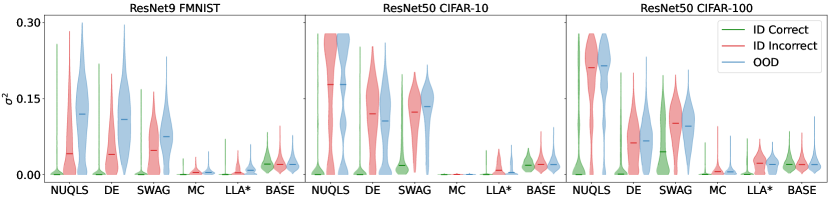
Figure 2: Violin plot of VMSP, for correctly predicted ID test points, incorrectly predicted ID test points, and OoD test points. Median is shown, with violin width depicting density. Low variance is expected for ID correct points, and large variance for ID incorrect and OoD points. Here FMNIST denotes FashionMNIST, MC denotes MC-Dropout, and BASE denotes Baseline.

Table 2: Image classification predictive performance, using LeNet5 on MNIST and FashionMNIST (FMNIST). Experiment was run $5$ times with different random MAP initialisations to get standard deviation on metrics.

Datasets	Method	NLL $\downarrow$	ACC $\uparrow$	ECE $\downarrow$	OOD-AUC $\uparrow$	AUC-ROC $\uparrow$	Time (s)
	MAP	$0.034\pm$$0.002$	$\mathbf{0.990\pm}$$\mathbf{0.001}$	$0.008\pm$$0.001$	$0.888\pm$$0.008$	$0.886\pm$$0.008$	$257$
	NUQLS	$0.035\pm$$0.002$	$0.989\pm$$0.001$	$\mathbf{0.003\pm}$$\mathbf{0.000}$	$\mathbf{0.930\pm}$$\mathbf{0.026}$	$\mathbf{0.928\pm}$$\mathbf{0.026}$	$106$
MNIST	DE	$0.034\pm$$0.004$	$\mathbf{0.991\pm}$$\mathbf{0.000}$	$0.011\pm$$0.004$	$\mathbf{0.932\pm}$$\mathbf{0.009}$	$\mathbf{0.928\pm}$$\mathbf{0.009}$	$2845$
	MC-Dropout	$0.044\pm$$0.002$	$0.989\pm$$0.000$	$0.017\pm$$0.01$	$0.873\pm$$0.032$	$0.871\pm$$0.031$	$533$
	SWAG	$\mathbf{0.029\pm}$$\mathbf{0.003}$	$\mathbf{0.991\pm}$$\mathbf{0.000}$	$\mathbf{0.004\pm}$$\mathbf{0.002}$	$0.902\pm$$0.008$	$0.900\pm$$0.008$	$489$
	LLA*	$0.034\pm$$0.002$	$\mathbf{0.990\pm}$$\mathbf{0.001}$	$0.008\pm$$0.001$	$0.888\pm$$0.008$	$0.886\pm$$0.008$	$45$
	VaLLA	$0.034\pm$$0.002$	$\mathbf{0.990\pm}$$\mathbf{0.001}$	$0.008\pm$$0.001$	$0.889\pm$$0.008$	$0.886\pm$$0.008$	$1583$
	MAP	$0.298\pm$$0.007$	$0.891\pm$$0.3$	$\mathbf{0.006\pm}$$\mathbf{0.001}$	$0.840\pm$$0.022$	$0.804\pm$$0.021$	$158$
	NUQLS	$0.302\pm$$0.006$	$0.891\pm$$0.002$	$\mathbf{0.005\pm}$$\mathbf{0.002}$	$\mathbf{0.904\pm}$$\mathbf{0.007}$	$\mathbf{0.870\pm}$$\mathbf{0.006}$	$89$
FMNIST	DE	$0.288\pm$$0.002$	$0.896\pm$$0.001$	$0.013\pm$$0.001$	$0.876\pm$$0.003$	$0.836\pm$$0.003$	$1587$
	MC-Dropout	$0.306\pm$$0.007$	$0.892\pm$$0.003$	$0.026\pm$$0.002$	$0.856\pm$$0.021$	$0.813\pm$$0.019$	$291$
	SWAG	$\mathbf{0.283\pm}$$\mathbf{0.005}$	$\mathbf{0.899\pm}$$\mathbf{0.003}$	$0.018\pm$$0.002$	$0.817\pm$$0.023$	$0.783\pm$$0.022$	$264$
	LLA*	$0.298\pm$$0.007$	$0.891\pm$$0.003$	$\mathbf{0.006\pm}$$\mathbf{0.001}$	$0.841\pm$$0.022$	$0.805\pm$$0.021$	$26$
	VaLLA	$0.298\pm$$0.007$	$0.891\pm$$0.003$	$0.007\pm$$0.001$	$0.841\pm$$0.022$	$0.805\pm$$0.021$	$1583$

5 Experiments

We now compare the performance of our method with alternatives on various regression and classification tasks. Implementation details are given in Appendix E. The PyTorch implementation of our experiments is available here.

5.1 Toy Regression

We compare the performance of our method on a toy regression problem, taken from (Hernández-Lobato & Adams, 2015) and extended in (Park & Blei, 2024). In Figure 1, we take $20$ uniformly sampled points in the domain $x\in[-4,-2]\cup[2,4]$, and let $y=x^{3}+\epsilon,~\epsilon\sim\mathcal{N}(0,3^{2})$. A small MLP was trained on these data and used for prediction. We apply VI, SWAG, LA, LLA, DE and NUQLS to the network to find a predictive mean and uncertainty. Close to the training data, i.e. in $[-4,-2]\cup[2,4]$ we expect low uncertainty; outside of this region, the uncertainty should grow with distance from the training points. VI underestimates, while SWAG and LA overestimate the uncertainty. DE grows more uncertain with distance from the training points, however both NUQLS and the LLA contain the underlying target curve within their confidence intervals. Note that deep ensembles output a heteroskedastic variance term, and were trained on a Gaussian likelihood; in comparison, the variances for LLA and NUQLS were computed post-hoc.

5.2 UCI Regression

In Tables 1 and 6, we compare NUQLS with DE, LLA and SWAG on a series of UCI regression problems. Mean squared error (MSE) and expected calibration error (ECE) respectively evaluate the predictive and UQ performance, with Gaussian negative log likelihood (NLL) evaluating both. See (Nemani et al., 2023a, $\S 4.11$) for an explanation of ECE. We see that NUQLS consistently has the (equal) best ECE (except for the Song dataset, where it falls short of the LLA ECE by $\mathit{0.1\%}$). It has comparable or better NLL than other methods on all datasets, and often gives an improvement on RMSE. Finally, it is the quickest method, often by a very significant margin, and it does not fail on any datasets, like the other methods do. Note that for the two largest datasets, Protein and Song, we required approximations on the covariance structure of LLA (see (Daxberger et al., 2021)). A detailed explanation of the hyper-parameter tuning method for NUQLS is given in Section C.1.

5.3 Image Classification - Uncertainty

In Figure 2, we compare the UQ performance of NUQLS, DE, SWAG, LLA* (LLA with a last-layer and KFAC approximation), and MC-Dropout, on larger image classification tasks. While previous works have measured the uncertainty quantification performance through entropy, ECE, and AUC-ROC, we propose a new metric. The previous measurements are all based on calibration of the softmax output for classification. However, the softmax probabilities are not a notion of uncertainty, but are instead a point prediction of class probability; uncertainty should accompany a point prediction, and quantify the spread of possible values. Instead, we propose to use the variance of the maximum predicted softmax probability (VMSP), for a given test point, as a better quantifier of uncertainty.

Figure 2 presents a violin plot of the VMSP for three test-groups: correctly predicted in-distribution (FashionMNIST, CIFAR-10) test points, incorrectly predicted in-distribution test points, and out-of distribution (MNIST, CIFAR-100) test points. We would expect that there should be smaller uncertainty for ID test points that have been correctly predicted, and larger uncertainty for incorrectly predicted ID and OoD test points. We compare against a completely randomized baseline method (BASE), where we sample $10$ standard normal realizations of logits, passed through a softmax. In Table 7 in Section D.6, we display the corresponding median values for each method in each test group. Ideally, a method should far outperform the baseline, so we can use the median difference between a method and the baseline as a way to compare different methods. We see that NUQLS performs as well as or better than all other methods, including the SOTA method DE. Furthermore, we would like the ID correct distribution to have a positive-skew, while ID incorrect and OoD distributions should have a negative-skew. We also display the sample skew values in Table 7. In this metric, our method again performs as well as or better than all other methods.

5.4 Image Classification - Predictive

We now evaluate the peformance of the novel predictive mean on image classification tasks. We compare NUQLS against the MAP NN, DE, MC-Dropout, SWAG, LLA* and VaLLA, on the MNIST and FashionMNIST datasets, using the LeNet5 network. We compare test cross-entropy (NLL), test accuracy (ACC), ECE, and the AUC-ROC measurement for maximum softmax probability (AUC-ROC) and entropy (OOD-AUC) as the detector. The last two metrics evaluate a methods ability to detect out-of distribution points. We display the results in Table 2. We see that NUQLS performs the best in ECE, AUC-ROC and OOD-AUC, and is competitive in the other metrics, while having the second fastest wall-time.

6 Conclusion

We have presented NUQLS, a Bayesian, post-hoc UQ method that approximates the predictive distribution of an over-parameterized NN through GD/SGD training of linear networks, allowing scalability without sacrificing performance. Under assumptions on the loss function, this predictive distribution reduces to a GP using the NTK. We find that our method is competitive with, and often far outperforms, existing UQ methods on regression and classification tasks, whilst providing a novel connection between NNs, GPs and the NTK. Potential future research could involve extending Theorem 3.2 to broader classes of loss functions and other deterministic and stochastic optimization algorithms.

Appendix A Proofs

Proof of Lemma 3.1.

First, we note that by the assumption on $\ell$, a solution to 5 always exists. Suppose to the contrary that 5 has two distinct solutions $\tilde{\bm{\theta}}$ and $\widehat{\bm{\theta}}$ such that $\tilde{\bm{\theta}}\neq\widehat{\bm{\theta}}$. Since $\tilde{\bm{\theta}}\in{\textnormal{Range}}([{\mathbf{J}}(\widehat{\bm{\theta}},\mathcal{X})]^{{{\mathchoice{\raisebox{0.0pt}{$\displaystyle\intercal$}}{\raisebox{0.0pt}{$\textstyle\intercal$}}{\raisebox{0.0pt}{$\scriptstyle\intercal$}}{\raisebox{0.0pt}{$\scriptscriptstyle\intercal$}}}}})$ and $\widehat{\bm{\theta}}\in{\textnormal{Range}}([{\mathbf{J}}(\widehat{\bm{\theta}},\mathcal{X})]^{{{\mathchoice{\raisebox{0.0pt}{$\displaystyle\intercal$}}{\raisebox{0.0pt}{$\textstyle\intercal$}}{\raisebox{0.0pt}{$\scriptstyle\intercal$}}{\raisebox{0.0pt}{$\scriptscriptstyle\intercal$}}}}})$, i.e., $(\tilde{\bm{\theta}}-\widehat{\bm{\theta}})\perp{\textnormal{Null}}([{\mathbf{J}}(\widehat{\bm{\theta}},\mathcal{X})])$, it follows that ${\mathbf{J}}(\widehat{\bm{\theta}},\mathcal{X})\tilde{\bm{\theta}}\neq{\mathbf{J}}(\widehat{\bm{\theta}},\mathcal{X})\widehat{\bm{\theta}}$, which in particular implies $\langle\nabla{\bf f}(\widehat{\bm{\theta}},{\bf x}_{i}),\tilde{\bm{\theta}}\rangle\neq\langle\nabla{\bf f}(\widehat{\bm{\theta}},{\bf x}_{i}),\widehat{\bm{\theta}}\rangle$ for all $i=1,\ldots,n$. Consider $\bar{\bm{\theta}}=(\tilde{\bm{\theta}}+\widehat{\bm{\theta}})/2$. By strict convexity on $\ell$, we have

$$\sum_{i=1}^{n}\ell(\widetilde{{\bf f}}(\bar{\bm{\theta}},{\bf x}_{i}),y_{i}) =\sum_{i=1}^{n}\ell\Bigg{(}{\bf f}(\widehat{\bm{\theta}},{\bf x}_{i})+\left\langle\nabla{\bf f}(\widehat{\bm{\theta}},{\bf x}_{i}),\frac{\tilde{\bm{\theta}}+\widehat{\bm{\theta}}}{2}-\widehat{\bm{\theta}}\right\rangle,y_{i}\Bigg{)}$$

$$=\sum_{i=1}^{n}\ell\Bigg{(}\frac{{\bf f}(\widehat{\bm{\theta}},{\bf x}_{i})+\left\langle\nabla{\bf f}(\widehat{\bm{\theta}},{\bf x}_{i}),\tilde{\bm{\theta}}-\widehat{\bm{\theta}}\right\rangle}{2}+\frac{{\bf f}(\widehat{\bm{\theta}},{\bf x}_{i})+\left\langle\nabla{\bf f}(\widehat{\bm{\theta}},{\bf x}_{i}),\widehat{\bm{\theta}}-\widehat{\bm{\theta}}\right\rangle}{2},y_{i}\Bigg{)}$$

$$<\frac{1}{2}\sum_{i=1}^{n}\ell\left(\widetilde{{\bf f}}(\tilde{\bm{\theta}},{\bf x}_{i}),y_{i}\right)+\frac{1}{2}\sum_{i=1}^{n}\ell\left(\widetilde{{\bf f}}(\widehat{\bm{\theta}},{\bf x}_{i}),y_{i}\right)$$

$$=\sum_{i=1}^{n}\ell\left(\widetilde{{\bf f}}(\tilde{\bm{\theta}},{\bf x}_{i}),y_{i}\right),$$

which is a contradiction. ∎

Proof of Theorem 3.2.

• (Gradient Descent) Denoting

  $${\mathbf{J}}(\widehat{\bm{\theta}},\mathcal{X})\triangleq\begin{bmatrix}{\mathbf{J}}^{{{\mathchoice{\raisebox{0.0pt}{$\displaystyle\intercal$}}{\raisebox{0.0pt}{$\textstyle\intercal$}}{\raisebox{0.0pt}{$\scriptstyle\intercal$}}{\raisebox{0.0pt}{$\scriptscriptstyle\intercal$}}}}}(\widehat{\bm{\theta}},{\bf x}_{1})\;\ldots\;{\mathbf{J}}^{{{\mathchoice{\raisebox{0.0pt}{$\displaystyle\intercal$}}{\raisebox{0.0pt}{$\textstyle\intercal$}}{\raisebox{0.0pt}{$\scriptstyle\intercal$}}{\raisebox{0.0pt}{$\scriptscriptstyle\intercal$}}}}}(\widehat{\bm{\theta}},{\bf x}_{n})\end{bmatrix}^{{{\mathchoice{\raisebox{0.0pt}{$\displaystyle\intercal$}}{\raisebox{0.0pt}{$\textstyle\intercal$}}{\raisebox{0.0pt}{$\scriptstyle\intercal$}}{\raisebox{0.0pt}{$\scriptscriptstyle\intercal$}}}}}\in^{nc\times p},$$

  we can write

  $${\bf z}={\mathbf{J}}^{\dagger}(\widehat{\bm{\theta}},\mathcal{X}){\mathbf{J}}(\widehat{\bm{\theta}},\mathcal{X}){\bf z}+\left(\mathbf{I}-{\mathbf{J}}^{\dagger}(\widehat{\bm{\theta}},\mathcal{X}){\mathbf{J}}(\widehat{\bm{\theta}},\mathcal{X})\right){\bf z},$$

  where $\widehat{\bm{\theta}}$ represents the parameters around which the linear model $\widetilde{{\bf f}}$ is defined in (2). The first iteration of gradient descent, initialized at $\bm{\theta}^{(0)}={\bf z}$, is given by

  $$\bm{\theta}^{(1)} ={\bf z}-\alpha\sum_{i=1}^{n}\frac{\partial\widetilde{{\bf f}}}{\partial\bm{\theta}}({\bf z},{\bf x}_{i})\nabla\ell(\widetilde{{\bf f}}({\bf z},{\bf x}_{i}),{\bf y}_{i})$$

  $$=\left(\mathbf{I}-{\mathbf{J}}^{\dagger}(\widehat{\bm{\theta}},\mathcal{X}){\mathbf{J}}(\widehat{\bm{\theta}},\mathcal{X})\right){\bf z}+{\mathbf{J}}^{\dagger}(\widehat{\bm{\theta}},\mathcal{X}){\mathbf{J}}(\widehat{\bm{\theta}},\mathcal{X}){\bf z}-\alpha\sum_{i=1}^{n}\frac{\partial\widetilde{{\bf f}}}{\partial\bm{\theta}}({\bf z},{\bf x}_{i})\nabla\ell(\widetilde{{\bf f}}({\bf z},{\bf x}_{i}),{\bf y}_{i})$$

  $$=\left(\mathbf{I}-{\mathbf{J}}^{\dagger}(\widehat{\bm{\theta}},\mathcal{X}){\mathbf{J}}(\widehat{\bm{\theta}},\mathcal{X})\right){\bf z}+{\mathbf{J}}^{\dagger}(\widehat{\bm{\theta}},\mathcal{X}){\mathbf{J}}(\widehat{\bm{\theta}},\mathcal{X}){\bf z}-\alpha\sum_{i=1}^{n}\left[{\mathbf{J}}(\widehat{\bm{\theta}},{\bf x}_{i})\right]^{{{\mathchoice{\raisebox{0.0pt}{$\displaystyle\intercal$}}{\raisebox{0.0pt}{$\textstyle\intercal$}}{\raisebox{0.0pt}{$\scriptstyle\intercal$}}{\raisebox{0.0pt}{$\scriptscriptstyle\intercal$}}}}}\nabla\ell(\widetilde{{\bf f}}({\bf z},{\bf x}_{i}),{\bf y}_{i})$$

  $$=\left(\mathbf{I}-{\mathbf{J}}^{\dagger}(\widehat{\bm{\theta}},\mathcal{X}){\mathbf{J}}(\widehat{\bm{\theta}},\mathcal{X})\right){\bf z}+{\bf v}^{(1)},$$

  where ${\bf v}^{(1)}\in{\textnormal{Range}}\left(\left[{\mathbf{J}}(\widehat{\bm{\theta}},\mathcal{X})\right]^{{{\mathchoice{\raisebox{0.0pt}{$\displaystyle\intercal$}}{\raisebox{0.0pt}{$\textstyle\intercal$}}{\raisebox{0.0pt}{$\scriptstyle\intercal$}}{\raisebox{0.0pt}{$\scriptscriptstyle\intercal$}}}}}\right)$. The next iteration is similarly given by

  $$\bm{\theta}^{(2)} =\bm{\theta}^{(1)}-\alpha\sum_{i=1}^{n}\frac{\partial\widetilde{{\bf f}}}{\partial\bm{\theta}}(\bm{\theta}^{(1)},{\bf x}_{i})\nabla\ell(\widetilde{{\bf f}}(\bm{\theta}^{(1)},{\bf x}_{i}),{\bf y}_{i})$$

  $$=\left(\mathbf{I}-{\mathbf{J}}^{\dagger}(\widehat{\bm{\theta}},\mathcal{X}){\mathbf{J}}(\widehat{\bm{\theta}},\mathcal{X})\right){\bf z}+{\bf v}^{(1)}-\alpha\sum_{i=1}^{n}\left[{\mathbf{J}}(\widehat{\bm{\theta}},{\bf x}_{i})\right]^{{{\mathchoice{\raisebox{0.0pt}{$\displaystyle\intercal$}}{\raisebox{0.0pt}{$\textstyle\intercal$}}{\raisebox{0.0pt}{$\scriptstyle\intercal$}}{\raisebox{0.0pt}{$\scriptscriptstyle\intercal$}}}}}\nabla\ell(\widetilde{{\bf f}}(\bm{\theta}^{(1)},{\bf x}_{i}),{\bf y}_{i})$$

  $$=\left(\mathbf{I}-{\mathbf{J}}^{\dagger}(\widehat{\bm{\theta}},\mathcal{X}){\mathbf{J}}(\widehat{\bm{\theta}},\mathcal{X})\right){\bf z}+{\bf v}^{(1)}+{\bf v}^{(2)},$$

  where again ${\bf v}^{(2)}\in{\textnormal{Range}}\left(\left[{\mathbf{J}}(\widehat{\bm{\theta}},\mathcal{X})\right]^{{{\mathchoice{\raisebox{0.0pt}{$\displaystyle\intercal$}}{\raisebox{0.0pt}{$\textstyle\intercal$}}{\raisebox{0.0pt}{$\scriptstyle\intercal$}}{\raisebox{0.0pt}{$\scriptscriptstyle\intercal$}}}}}\right)$. Generalizing to the $n$th iteration,

  $$\bm{\theta}^{(n)} =\left(\mathbf{I}-{\mathbf{J}}^{\dagger}(\widehat{\bm{\theta}},\mathcal{X}){\mathbf{J}}(\widehat{\bm{\theta}},\mathcal{X})\right){\bf z}+\sum_{i=1}^{n}{\bf v}^{(i)}.$$

  Hence, by the assumption on $\ell$, as long as an adaptive learning rate is chosen appropriately according to Malitsky & Mishchenko (2020), GD must converge to a solution of the form

  $$\bm{\theta}^{\star} =\left(\mathbf{I}-{\mathbf{J}}^{\dagger}(\widehat{\bm{\theta}},\mathcal{X}){\mathbf{J}}(\widehat{\bm{\theta}},\mathcal{X})\right){\bf z}+\sum_{i=1}^{\infty}{\bf v}^{(i)}$$

  $$=\left(\mathbf{I}-{\mathbf{J}}^{\dagger}(\widehat{\bm{\theta}},\mathcal{X}){\mathbf{J}}(\widehat{\bm{\theta}},\mathcal{X})\right){\bf z}+{\bf v},$$

  where ${\bf v}\in{\textnormal{Range}}\left(\left[{\mathbf{J}}(\widehat{\bm{\theta}},\mathcal{X})\right]^{{{\mathchoice{\raisebox{0.0pt}{$\displaystyle\intercal$}}{\raisebox{0.0pt}{$\textstyle\intercal$}}{\raisebox{0.0pt}{$\scriptstyle\intercal$}}{\raisebox{0.0pt}{$\scriptscriptstyle\intercal$}}}}}\right)$. In particular, for ${\bf z}={\bf 0}$, by Lemma 3.1, we must have that ${\bf v}=\bm{\theta}^{\ddagger}$, where $\bm{\theta}^{\ddagger}$ is the solution to 5. Therefore,

  $$\bm{\theta}^{\star} =\left(\mathbf{I}-{\mathbf{J}}^{\dagger}(\widehat{\bm{\theta}},\mathcal{X}){\mathbf{J}}(\widehat{\bm{\theta}},\mathcal{X})\right){\bf z}+\bm{\theta}^{\ddagger}.$$

• (Stochastic Gradient Descent) Using a similar argument as above, it is easy to show that each iteration of the mini-batch SGD is of the form

  $$\bm{\theta}^{(n)}\in\left(\mathbf{I}-{\mathbf{J}}^{\dagger}(\widehat{\bm{\theta}},\mathcal{X}){\mathbf{J}}(\widehat{\bm{\theta}},\mathcal{X})\right){\bf z}+{\textnormal{Range}}\left(\left[{\mathbf{J}}(\widehat{\bm{\theta}},\mathcal{X})\right]^{{{\mathchoice{\raisebox{0.0pt}{$\displaystyle\intercal$}}{\raisebox{0.0pt}{$\textstyle\intercal$}}{\raisebox{0.0pt}{$\scriptstyle\intercal$}}{\raisebox{0.0pt}{$\scriptscriptstyle\intercal$}}}}}\right).$$

  Hence, it suffices to show that SGD converges almost surely. Defining

  $$\mathcal{L}(\bm{\theta})\triangleq\sum_{i=1}^{n}\ell(\widetilde{{\bf f}}(\bm{\theta},{\bf x}_{i}),{\bf y}_{i}),\quad\text{and}\quad{\bf g}(\bm{\theta},\mathcal{X})\triangleq\begin{bmatrix}\nabla\ell(\widetilde{{\bf f}}(\bm{\theta},{\bf x}_{1}),{\bf y}_{1})\\ \vdots\\ \nabla\ell(\widetilde{{\bf f}}(\bm{\theta},{\bf x}_{n}),{\bf y}_{n})\end{bmatrix}\in^{nc},$$

  we write

  $$\nabla\mathcal{L}(\bm{\theta})=\sum_{i=1}^{n}\left[{\mathbf{J}}(\widehat{\bm{\theta}},{\bf x}_{1})\right]^{{{\mathchoice{\raisebox{0.0pt}{$\displaystyle\intercal$}}{\raisebox{0.0pt}{$\textstyle\intercal$}}{\raisebox{0.0pt}{$\scriptstyle\intercal$}}{\raisebox{0.0pt}{$\scriptscriptstyle\intercal$}}}}}\nabla\ell(\widetilde{{\bf f}}(\bm{\theta},{\bf x}_{i}),{\bf y}_{i})=\left[{\mathbf{J}}(\widehat{\bm{\theta}},\mathcal{X})\right]^{{{\mathchoice{\raisebox{0.0pt}{$\displaystyle\intercal$}}{\raisebox{0.0pt}{$\textstyle\intercal$}}{\raisebox{0.0pt}{$\scriptstyle\intercal$}}{\raisebox{0.0pt}{$\scriptscriptstyle\intercal$}}}}}{\bf g}(\bm{\theta},\mathcal{X}).$$

  Let $\bm{\theta}^{\star}$ be any solution to 3. The full row-rank assumption on ${\mathbf{J}}(\widehat{\bm{\theta}},\mathcal{X})$ implies that we must have ${\bf g}(\bm{\theta}^{\star},\mathcal{X})={\bf 0}$, i.e., $\nabla\ell(\widetilde{{\bf f}}(\bm{\theta}^{\star},{\bf x}_{i}),{\bf y}_{i})={\bf 0}$, $i=1,\ldots,n$. By the $\mu$-strong convexity assumption on $\ell(.,{\bf y})$ with respect to its first argument, it is easy to see that $\mathcal{L}(\bm{\theta})$ satisfies the Polyak-Łojasiewicz inequality (Karimi et al., 2016) with constant $2\mu\lambda$ where

  $$\lambda\triangleq\min_{i=1,\ldots,n}\sigma^{2}_{\min}({\mathbf{J}}(\widehat{\bm{\theta}},{\bf x}_{i})),$$

  and $\sigma_{\min}({\mathbf{J}}(\widehat{\bm{\theta}},{\bf x}_{i}))$ is the smallest non-zero singular value of ${\mathbf{J}}(\widehat{\bm{\theta}},{\bf x}_{i})$. Indeed, let $\bm{\theta}^{\star}$ be any solution to 3. From $\mu$-strong convexity of $\ell(.,{\bf y})$ with respect to its first argument, for any $\bm{\theta}$, we have

  $$\ell(\widetilde{{\bf f}}(\bm{\theta},{\bf x}_{i}),{\bf y}_{i})-\ell(\widetilde{{\bf f}}(\bm{\theta}^{\star},{\bf x}_{i}),{\bf y}_{i}) \leq\frac{1}{2\mu}\left\|\nabla\ell(\widetilde{{\bf f}}(\bm{\theta},{\bf x}_{i}),{\bf y}_{i})\right\|^{2}$$

  $$\leq\frac{1}{2\mu\sigma_{\min}({\mathbf{J}}(\widehat{\bm{\theta}},{\bf x}_{i}))}\left\|\left[{\mathbf{J}}(\widehat{\bm{\theta}},{\bf x}_{i})\right]^{{{\mathchoice{\raisebox{0.0pt}{$\displaystyle\intercal$}}{\raisebox{0.0pt}{$\textstyle\intercal$}}{\raisebox{0.0pt}{$\scriptstyle\intercal$}}{\raisebox{0.0pt}{$\scriptscriptstyle\intercal$}}}}}\nabla\ell(\widetilde{{\bf f}}(\bm{\theta},{\bf x}_{i}),{\bf y}_{i})\right\|^{2},$$

  which implies

  $$\mathcal{L}(\bm{\theta})-\mathcal{L}(\bm{\theta}^{\star}) \leq\frac{1}{2\mu\lambda}\left\|\left[{\mathbf{J}}(\widehat{\bm{\theta}},\mathcal{X})\right]^{{{\mathchoice{\raisebox{0.0pt}{$\displaystyle\intercal$}}{\raisebox{0.0pt}{$\textstyle\intercal$}}{\raisebox{0.0pt}{$\scriptstyle\intercal$}}{\raisebox{0.0pt}{$\scriptscriptstyle\intercal$}}}}}{\bf g}(\bm{\theta},\mathcal{X})\right\|^{2}=\frac{1}{2\mu\lambda}\left\|\nabla\mathcal{L}(\bm{\theta})\right\|^{2}.$$

  By the smoothness assumption on each $\ell(\widetilde{{\bf f}}(.,{\bf x}_{i}),{\bf y}_{i})$ as well as the interpolating property of $\bm{\theta}^{\star}$, Bassily et al. (2018, Theorem 1) implies that the mini-batch SGD with small enough step size $\eta$ has an exponential convergence rate as

  $${\mathbb{E}}\mathcal{L}(\bm{\theta}^{(k)}) \leq(1-\rho)^{k}\mathcal{L}(\bm{\theta}^{(0)}),$$

  for some contact $0<\rho<1$. This in particular implies that for any $\epsilon>0$,

  $$\sum_{k=1}^{\infty}{\mathbb{P}}(\mathcal{L}(\bm{\theta}^{(k)})>\epsilon)\leq\sum_{k=1}^{\infty}\frac{{\mathbb{E}}\mathcal{L}(\bm{\theta}^{(k)})}{\epsilon}\leq\frac{\mathcal{L}(\bm{\theta}^{(0)})}{\epsilon}\sum_{k=1}^{\infty}(1-\rho)^{k}=\frac{\mathcal{L}(\bm{\theta}^{(0)})}{\epsilon\rho}<\infty.$$

  Now, the Borel–Cantelli lemma gives $\mathcal{L}(\bm{\theta}^{(k)})\to 0$, almost surely.

∎

Appendix B Related Works: Further Details and Discussions

NUQLS shares notable similarities with, and exhibits distinct differences from, several prior works, which are briefly discussed below.

B.1 Linearized Laplace Approximation (LLA) Framework.

The popular LLA framework (Khan et al., 2019; Foong et al., 2019; Immer et al., 2021; Daxberger et al., 2021) shares a close connection with NUQLS, as both methods fundamentally rely on linearizing the network. However, a subtle yet significant distinction lies in their constructions: LLA begins by obtaining a proper distribution over the parameters and then draws parameter samples from it, while NUQLS bypasses this step and directly targets an approximation of the posterior distribution of the neural network.

As a direct consequence of this, in overparameterized settings, where the Hessian (or its Generalized Gauss-Newton approximation) is not positive definite, the LLA framework necessitates imposing an appropriate prior over the parameters to avoid degeneracy. In sharp contrast, NUQLS directly generates samples from the predictive distribution without introducing any artificial prior, thereby avoiding potential biases that such priors might impose on the covariance structure of the outputs and eliminating the need for additional hyperparameters. Consequently, as the LLA framework corresponds to a Bayesian generalized linear model (GLM), the weight-space vs. function-space duality in GLMs implies that its predictive distribution corresponds to a noisy GP with an NTK kernel. On the other hand, NUQLS leads to a noise-free GP. In interpolating regimes, where the model perfectly fits the data, the noise-free setting of NUQLS appears to be more suitable (Hodgkinson et al., 2023).

Another important consequence of this distinction arises in classification tasks. Due to the Laplace approximation, the LLA framework produces an independent GP for each output of the linearized model. In contrast, NUQLS captures the covariance between outputs, offering a more comprehensive representation of the predictive distribution.

Finally, for regression tasks, NUQLS offers additional flexibility by allowing the variance to be scaled post-hoc by a factor $\gamma$. This enables efficient hyperparameter tuning on a validation set without the need for retraining the model or optimizing a marginal likelihood–a level of flexibility not available in the LLA framework.

NUQLS can be seen as an extension of the “sample-then-optimize” framework for posterior sampling of large, finite-width NNs (Matthews et al., 2017). In this context, the work of Antorán et al. (2022), henceforth referred to as Sampling-LLA, enables drawing samples from the posterior distribution of the LLA in a manner analogous to Algorithm 1. In this approach, a series of regularized least-squares regression problems are constructed, and the collection of their solutions is shown to be distributed according to the LLA posterior. An EM algorithm is then employed for hyperparameter tuning. In addition to the fundamental differences between NUQLS and LLA-inspired methods mentioned earlier, Sampling-LLA has notable distinctions from Algorithm 1. First, the objective functions in Sampling-LLA have non-trivial minimum values. As a result, the convergence of SGD for such problems necessitates either a diminishing learning rate (Bubeck et al., 2015), which slows down convergence, or the adoption of variance reduction techniques (Roux et al., 2012; Shalev-Shwartz & Zhang, 2013; Johnson & Zhang, 2013), which can introduce additional computational and memory overhead. By contrast, in overparameterized settings and under the assumptions of Theorem 3.2, the optimization problem in 3 allows interpolation. Consequently, SGD can employ a constant step size for convergence, improving optimization efficiency (Garrigos & Gower, 2023). Second, the inherent properties of the LLA framework, which require a positive definite Hessian or its approximation, necessitate regularizing the least-squares term in the subproblem of Sampling-LLA. This results in a strongly convex problem with a unique solution. Consequently, to generate a collection of solutions, Sampling-LLA constructs a random set of such subproblems, each involving fitting the linearized network to random outputs. These random outputs are sampled from a zero-mean Gaussian, with covariance given by the Hessian of the loss function, evaluated on the data. In contrast, the subproblem of NUQLS, i.e., 3, involves directly fitting the training data, and the ensemble of solutions is constructed as a result of random initialization of the optimization algorithm. Hence, the uncertainty captured by NUQLS arises naturally from the variance of solutions in the overparameterized regime, without the need for additional regularization or artificially constructed subproblems.

While the Sampling-LLA method enhances the scalability of LLA, the competing method Variational LLA (VaLLA) (Ortega et al., 2023) offers comparable or superior UQ performance while significantly reducing computation time. VaLLA achieves this by computing the LLA predictive distribution using a variational sparse GP with an NTK. Another competing LLA extension is Accelerated LLA (ELLA), which uses a Nyström approximation of the functional LLA covariance matrix (Deng et al., 2022), and seems to attain similar performance to VaLLA, again at a reduced cost compared to Sampling-LLA. We compare the performance of NUQLS to Sampling-LLA, VaLLA and ELLA in Section D.2.

B.2 Ensemble Framework.

In Lee et al. (2019), infinitely wide neural networks were shown to follow a GP distribution; however, this GP did not correspond to a true predictive distribution. Building on this, He et al. (2020) introduced a random, untrainable function to an infinitely wide neural network, deriving a GP predictive distribution using the infinite-width NTK. An ensemble of these modified NNs was then interpreted as samples from the GP’s predictive posterior. In contrast, our method demonstrates that trained, finite-width, unmodified linearized networks are inherently samples from a GP with an NTK kernel. While their method, Bayesian Deep Ensembles (BDE), shares some conceptual similarities with ours, we omit it from our experiments for several reasons. Firstly, while it performed well in a toy regression problem in the original paper, it performed poorly on the alternate toy regression problem found in Figure 4 in Section D.3; this is likely due to the infinite-width NTK being a poor approximation in practice. Second, the method is computationally more expensive than DE, particularly for classification tasks, where it requires additional parameter tuning on a validation set. Since our goal is to provide a UQ method that is more computationally efficient than the state-of-the-art SOTA method DE while maintaining competitive performance, BDE is not considered a suitable candidate for comparison.

In Madras et al. (2019), the authors propose a method called “local ensembles”, which perturbs the parameters of a trained network along directions of small loss curvature to create an ensemble of nearly loss-invariant networks. The uncertainty of the original network is then quantified as the standard deviation across predictions in the ensemble. Building on this approach, Miani et al. (2024), in a method called Sketched Lanczos Uncertainty (SLU), use the GGN approximation of the Hessian of the loss to identify these directions and introduce a sketched Lanczos algorithm (Meurant, 2006) to efficiently compute them. We compare the performance of NUQLS to SLU in Section D.1.

While similar, there are key differences between local ensembles and NUQLS. Local ensembles form a subspace of networks that attain similar loss values, allowing for directions with small but non-zero curvature, potentially encompassing more directions than those with exactly zero curvature. In contrast, when a solution to the linear optimization problem exists, NUQLS creates an ensemble of networks that all attain exactly the same loss. Additionally, NUQLS relies on first-order information to construct this ensemble, whereas local ensembles depend on second-order information.

While the zero-curvature directions of the GGN approximation correspond to the Jacobian’s null space, the local ensembles method also includes directions with small but non-zero curvature. This inclusion introduces a notable distinction between the ensembles generated by local ensembles and those formed by NUQLS. Finally, while local ensembles employ low-rank approximations to compute directions efficiently, such approximations may inadequately represent the Hessian and fail to accurately capture the true curvature structure, as highlighted in Xie et al. (2022).

Appendix C Hyper-parameter Tuning

NUQLS contains several hyper-parameters: the number of linear networks to be trained, the number of epochs and learning rate of training, and the variance of initialisation, $\gamma$. In this section, we discuss strategies to select optimal hyper-parameters.

C.1 Regression

For regression, and with a sufficiently small learning rate, NUQLS samples from the distribution given in Remark 3.3. We can see that the variance of the predictions scales linearly with $\gamma^{2}$. Hence, we use the following framework to tune $\gamma$:

1. To obtain $\bm{\theta}_{s}$ in Algorithm 1, we initialise our parameters with a very small gamma, e.g. $\gamma=0.01$. This enables (stochastic) gradient descent to converge quickly with a small learning rate.

2. We compute $\{\widetilde{{\bf f}}(\bm{\theta}^{\star}_{s},\mathcal{X}_{\text{val}})\}_{s=1}^{S}$, where $\mathcal{X}_{\text{val}}$ is the inputs from a validation set. As per Remark 3.3, for each point ${\bf x}\in\mathcal{X}_{\text{val}}$, we compute the mean prediction as $\mu(x)=\text{SampleMean}\left(\{\widetilde{{\bf f}}(\bm{\theta}^{\star}_{s},{\bf x})\}_{s=1}^{S}\right)$ and the variance as $\sigma^{2}_{\gamma}(x)=\text{SampleVariance}\left(\{\gamma\widetilde{{\bf f}}(\bm{\theta}^{\star}_{s},\mathcal{X}_{\text{val}})\}_{s=1}^{S}\right)$ (note the scaling by $\gamma$ for only the variance). We then use these values to compute the ECE across the validation dataset $\mathcal{D}_{\text{val}}$.

3. As coverage of a confidence interval scales linearly with the size of the given standard deviation, and our computed standard deviation scales linearly with $\gamma$, we find that the ECE is convex in $\gamma$. Hence, we employ the Ternary search method (see Algorithm 2) to find the value $\hat{\gamma}$ that minimizes this validation ECE.

4. For a test point ${\bf x}^{\star}$, our mean prediction and variance is then $\mu({\bf x}^{\star})$ and $\sigma^{2}_{\hat{\gamma}}({\bf x}^{\star})$.

As can be seen in Table 1 and Table 6, this framework means that for regression our method is incredibly fast and computes well-calibrated variance values.

Algorithm 2 Ternary Search

 $f$: function to minimize, $l$: left boundary of search space, $r$: right boundary of search space, $\delta$: tolerance, iter: iterations.

 $i=0$

 while $|l-r|\geq\delta$ and $i<$iter do

  $l_{1/3}=l+(r-l)/3$

  $r_{1/3}=r-(r-l)/3$

  if $f(l_{1/3})<f(r_{1/3})$ then

   $l=l_{1/3}$

  else

   $r=r_{1/3}$

  end if

 end while

 return  $(l+r)/2$

C.2 Classification

For classification, with cross-entropy loss, there is no principled connection to a GP, nor a clean calibration method as in Section C.1. Instead, we propose some heuristics for how to choose the hyper-parameters of NUQLS. To accomplish this, we train a LeNet model on both MNIST and FashionMNIST, and run NUQLS on the trained model for a variety of learning rates, epochs and values of $\gamma$. We measure training loss of NUQLS, accuracy, ECE, AUC-ROC and OOD-AUC, as well as the training loss of the NN. We repeat this for $5$ random initialisations, and plot the average results in Figure 3.

Looking at Figure 3, we see that for loss values under the training loss of the original NN, performance is quite similar. Furthermore, for loss values over the training loss of the NN, a higher learning rate and number of epochs seems to equate to better performance. Finally, greater loss values, up to a threshold, seem to increase the OoD detection performance (measured by AUC-ROC and OOD-AUC). Greater loss values may equate to greater deviation in the row-space components of the ensemble solutions; this extra variance may help uncertainty quantification performance, though calibration for ID points seems to decrease (as measured by ECE).

We propose the following heuristic for hyper-parameter selection:

• For a set learning rate and number of epochs, choose the largest $\gamma$ such that the NUQLS training loss is less than the NN training loss.

• Parameter combinations such that the NUQLS training loss is moderately greater than the NN training loss may be better for uncertainty quantification purposes, thought the predictive calibration may be worse.

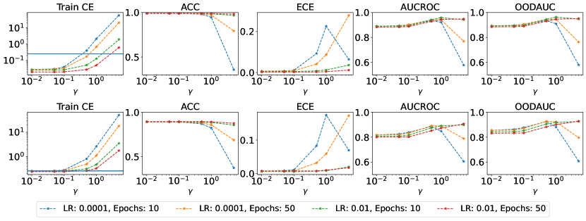
Figure 3: Comparison of NUQLS performance as a function of learning rate, epochs and standard deviation of initialisation $\gamma$. We train a LeNet model on (top) MNIST and (bottom) FashionMNIST, and compute a range of metrics. The results are averaged over $5$ random seeds. The blue horizontal line corresponds to the final training loss of the LeNet model.

Appendix D Further Experimental Results

D.1 Comparison to SLU

Here we compare the performance of our method against the competing SLU method. See Appendix B for a discussion of the differences between NUQLS and SLU. Due to the extensive experimental details given in (Miani et al., 2024), we run certain experiments from this work and report the performance of NUQLS against the SLU results found in (Miani et al., 2024). In Table 3, we compare NUQLS against SLU on OoD detection using the AUC-ROC metric, on a smaller single-layer MLP and a larger LeNet model. The MLP is trained on the MNIST dataset, while the LeNet model is trained on the FashionMNIST dataset. For MNIST, the OoD datasets are FashionMNIST, KMNIST, and a Rotated MNIST dataset, where for each experiment run, we compute the average AUC-ROC score over a range of rotation angles $(15,30,45,60,75,90,105,120,135,150,165,180)$. For FashionMNIST, the OoD datasets are MNIST, and the average Rotated FashionMNIST dataset. The AUC-ROC metric was calculated using the variance of the logits, summed over the classes for each test point, as a score. We observe that NUQLS has a better AUC-ROC value over all OoD datasets, often by a significant margin.

Table 3: Comparing performance of NUQLS against SLU method. Metric given is the AUC-ROC, computed using the variance of the logits, summed over the classes for each test point, as a score. AUC-ROC measures ability of a method to differentiate between ID and OoD points. We see that NUQLS out-performs SLU in these experiments.

Model	MLP $p=15k$			LeNet $p=40k$
ID Data	MNIST vs			FashionMNIST
OoD Data	FashionMNIST	KMNIST	Rotation (avg)	MNIST	Rotation (avg)
SLU	$0.26\pm$$0.02$	$0.42\pm$$0.04$	$0.59\pm$$0.02$	$\mathbf{0.94\pm}$$\mathbf{0.01}$	$0.74\pm$$0.03$
NUQLS	$\mathbf{0.67\pm}$$\mathbf{0.07}$	$\mathbf{0.79\pm}$$\mathbf{0.02}$	$\mathbf{0.74\pm}$$\mathbf{0.01}$	$\mathbf{0.95\pm}$$\mathbf{0.02}$	$\mathbf{0.91\pm}$$\mathbf{0.01}$

D.2 Comparison to Sampling-LLA, VaLLA and ELLA

We now compare NUQLS against Sampling-LLA, VaLLA and ELLA. Due to issues with convergence, performance, memory usage and package compatibility when either running source code or implementing methods from instructions given in (Antorán et al., 2022) and (Ortega et al., 2023), we instead compare NUQLS against the results for Sampling-LLA, VaLLA and ELLA taken verbatim from (Ortega et al., 2023, Figure 3). We train a $2$-layer MLP, with $200$ hidden-units in each layer, on the MNIST dataset, according to the experimental details given in (Ortega et al., 2023). We then compare the accuracy, NLL, ECE, Brier score and the OOD-AUC metric of NUQLS against those reported for Sampling-LLA, VaLLA and ELLA. The results are shown in Table 4. We display the mean and standard deviation for NUQLS; as is quoted in (Ortega et al., 2023), the standard deviation for the other methods was below $10^{-4}$ in magnitude, and was thus omitted. We see that NUQLS outperforms Sampling-LLA, VaLLA and ELLA in accuracy, NLL, ECE, and Brier score, and is within one-sixth of a standard deviation of the leading OOD-AUC value, attained by Sampling-LLA. While we cannot directly comment on differences in computation time between our method and these LLA extensions, we were able to run the source code for VaLLA for the experiments in Table 2, where NUQLS was an order-of-magnitude faster than VaLLA in wall-time. In (Ortega et al., 2023, Figure 3 (right)), we also observe that VaLLA is an order-of-magnitude faster than both Sampling-LLA and ELLA. We also compare with (Ortega et al., 2023, Table 1), where a ResNet20 model is trained on CIFAR-10. The results are displayed in Table 5. We see that NUQLS is competitive with all other methods in this setting.

Table 4: Comparing performance of NUQLS against Sampling-LLA, VaLLA and ELLA on MNIST, trained used a 2-layer MLP with $200$ hidden units in each layer, and $\tanh$ activation. Original results taken from (Ortega et al., 2023).

Model	ACC	NLL	ECE	BRIER	OOD-AUC
ELLA	$97.6$	$0.076$	$0.008$	$0.036$	$0.905$
Sampled LLA	$97.6$	$0.087$	$0.026$	$0.040$	$\mathbf{0.954}$
VaLLA 100	$97.7$	$0.076$	$0.010$	$0.036$	$0.916$
VaLLA 200	$97.7$	$0.075$	$0.010$	$0.035$	$0.921$
NUQLS	$\mathbf{98.0\pm}$$\mathbf{0.1}$	$\mathbf{0.065\pm}$$\mathbf{0.003}$	$\mathbf{0.005\pm}$$\mathbf{0.001}$	$\mathbf{0.031\pm}$$\mathbf{0.001}$	$\mathbf{0.953\pm}$$\mathbf{0.006}$

Table 5: Comparing performance of NUQLS against Sampling-LLA, VaLLA and ELLA on CIFAR-10, with ResNet20. Original results taken from (Ortega et al., 2023).

Model	ACC	NLL	ECE
ELLA	$92.5$	$0.233$	$0.009$
Sampled LLA	$92.5$	$0.231$	$\mathbf{0.006}$
VaLLA	$\mathbf{92.6}$	$\mathbf{0.228}$	$0.007$
NUQLS	$92.4\pm$$0.1$	$0.236\pm$$0.001$	$0.008\pm$$0.001$

D.3 Toy Regression BDE

Figure 4 displays the performance of BDE on the toy regression problem from Figure 1.

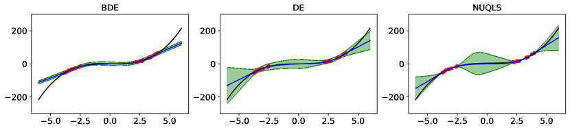
Figure 4: Comparison of BDE, DE and NUQLS on the toy regression problem from Figure 1. We can see that the uncertainty of the BDE method is quite small.

D.4 UCI Regression

We present the results for select UCI regression datasets in Table 1 in the main body; we present results for several more datasets in Table 6.

Table 6: Comparing performance of NUQLS, DE, LLA and SWAG on UCI regression tasks. NUQLS performs as well as or better than all other methods, while showing a speed up over other methods; this speed up increases with the size of the datasets. Note that for the Song dataset, the LLA method uses a diagonal covariance structure due to memory constraints: this is denoted as LLA-D.

Dataset	Method	RMSE $\downarrow$	NLL $\downarrow$	ECE $\downarrow$	Time(s)
Concrete	NUQLS	$\mathbf{0.330\pm}$$\mathbf{0.047}$	$\mathbf{-0.316\pm}$$\mathbf{0.501}$	$\mathbf{0.003\pm}$$\mathbf{0.001}$	$\mathbf{0.185}$
	DE	$0.379\pm$$0.019$	$\mathbf{-0.574\pm}$$\mathbf{0.098}$	$\mathbf{0.002\pm}$$\mathbf{0.002}$	$29.047$
	LLA	$\mathbf{0.333\pm}$$\mathbf{0.050}$	$\mathbf{-0.294\pm}$$\mathbf{0.479}$	$\mathbf{0.003\pm}$$\mathbf{0.002}$	$0.297$
	SWAG	$\mathbf{0.334\pm}$$\mathbf{0.050}$	$\mathbf{-0.562\pm}$$\mathbf{0.224}$	$0.009\pm$$0.006$	$36.262$
Naval	NUQLS	$\mathbf{0.049\pm}$$\mathbf{0.012}$	$\mathbf{-2.546\pm}$$\mathbf{0.134}$	$\mathbf{0.002\pm}$$\mathbf{0.002}$	$\mathbf{0.295}$
	DE	$0.076\pm$$0.006$	$-1.761\pm$$0.250$	$0.093\pm$$0.040$	$96.570$
	LLA	$0.070\pm$$0.022$	$25.292\pm$$17.570$	$0.192\pm$$0.029$	$129.659$
	SWAG	$1.130\pm$$1.500$	$0.303\pm$$1.091$	$0.084\pm$$0.022$	$92.662$
CCPP	NUQLS	$0.244\pm$$0.008$	$-0.885\pm$$0.020$	$\mathbf{0.000\pm}$$\mathbf{0.000}$	$\mathbf{0.174}$
	DE	$\mathbf{0.227\pm}$$\mathbf{0.006}$	$\mathbf{-1.009\pm}$$\mathbf{0.041}$	$\mathbf{0.002\pm}$$\mathbf{0.003}$	$79.791$
	LLA	$0.243\pm$$0.007$	$29.420\pm$$4.565$	$0.163\pm$$0.008$	$32.048$
	SWAG	$0.252\pm$$0.012$	$-0.849\pm$$0.038$	$\mathbf{0.001\pm}$$\mathbf{0.002}$	$66.833$
Wine	NUQLS	$\mathbf{0.789\pm}$$\mathbf{0.042}$	$\mathbf{0.284\pm}$$\mathbf{0.066}$	$\mathbf{0.001\pm}$$\mathbf{0.000}$	$\mathbf{0.115}$
	DE	$\mathbf{0.789\pm}$$\mathbf{0.041}$	$\mathbf{0.320\pm}$$\mathbf{0.109}$	$\mathbf{0.001\pm}$$\mathbf{0.001}$	$13.241$
	LLA	$\mathbf{0.792\pm}$$\mathbf{0.041}$	$1.012\pm$$0.182$	$0.009\pm$$0.004$	$0.340$
	SWAG	$\mathbf{0.798\pm}$$\mathbf{0.038}$	$\mathbf{0.367\pm}$$\mathbf{0.103}$	$0.005\pm$$0.003$	$11.807$
Yacht	NUQLS	$\mathbf{0.042\pm}$$\mathbf{0.013}$	$\mathbf{-1.561\pm}$$\mathbf{2.319}$	$\mathbf{0.012\pm}$$\mathbf{0.010}$	$\mathbf{0.164}$
	DE	$0.647\pm$$0.121$	$-2.032\pm$$0.349$	$\mathbf{0.016\pm}$$\mathbf{0.008}$	$40.132$
	LLA	$\mathbf{0.043\pm}$$\mathbf{0.014}$	$\mathbf{-2.733\pm}$$\mathbf{0.468}$	$\mathbf{0.011\pm}$$\mathbf{0.006}$	$0.177$
	SWAG	$\mathbf{0.044\pm}$$\mathbf{0.014}$	$-2.565\pm$$0.118$	$0.067\pm$$0.025$	$15.822$
Song	NUQLS	$\mathbf{0.839\pm}$$\mathbf{0.014}$	$0.646\pm$$0.056$	$0.001\pm$$0.000$	$\mathbf{91.673}$
	DE	$\mathbf{0.846\pm}$$\mathbf{0.006}$	$\mathbf{0.180\pm}$$\mathbf{0.013}$	$0.005\pm$$0.000$	$2562.789$
	LLA-D	$\mathbf{0.851\pm}$$\mathbf{0.029}$	$0.456\pm$$0.093$	$\mathbf{0.000\pm}$$\mathbf{0.000}$	$210.429$
	SWAG	$0.845\pm$$0.002$	$0.680\pm$$0.062$	$0.003\pm$$0.001$	$3274.440$

D.5 eNUQLS

In Figure 5 we demonstrate the performance of an ensembled version of NUQLS, eNUQLS. This method is similar to a Mixture of Laplace Approximations (Eschenhagen et al., 2021). We observe excellent separation of the variances between correct and incorrect/OoD test groups for eNUQLS, especially for CIFAR-10 on ResNet9. Note that there is significant cost to ensembling our method, and we provide this figure simply to illustrate performance capacity.

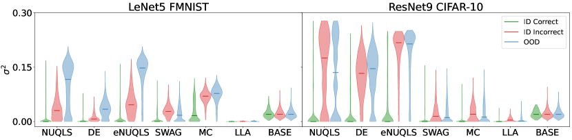
Figure 5: Violin plot of VMSP, with an ensembled version of NUQLS, eNUQLS, included.

D.6 Image Classification

The median and sample skew for the VMSP in Figure 2 is found in Table 7.

Table 7: Sample median and sample skew of variance from Figure 2. IDC = ID correct, IDIC = ID incorrect, FMNIST = FashionMNIST. The median and skew for a method is compared against a baseline method. We expect positive skew for the ID correct (IDC) variances, and a negative skew for the ID incorrect (IDIC) and OoD variances. If the median or skew for a method is worse than the corresponding baseline, then it is written in gray.

Median		NUQLS	DE	SWAG	MC	LLA	BASE
ResNet9	IDC $\downarrow$	$2.45\times 10^{-8}$	$1.31\times 10^{-5}$	$4.64\times 10^{-7}$	$5.05\times 10^{-7}$	$9.02\times 10^{-10}$	$0.020$
FMNIST	IDIC $\uparrow$	$0.041$	$0.040$	$0.048$	$\color[rgb]{.5,.5,.5}$	$\color[rgb]{.5,.5,.5}$	$0.020$
	OoD $\uparrow$	$0.119$	$0.109$	$0.075$	$\color[rgb]{.5,.5,.5}$	$\color[rgb]{.5,.5,.5}$	$0.020$
ResNet50	IDC $\downarrow$	$0.00$	$8.29\times 10^{-8}$	$0.018$	$1.49\times 10^{-9}$	$1.70\times 10^{-7}$	$0.019$
CIFAR-10	IDIC $\uparrow$	$0.178$	$0.120$	$0.123$	$\color[rgb]{.5,.5,.5}{1.32\times 10^{-4}}$	$\color[rgb]{.5,.5,.5}$	$0.020$
	OoD $\uparrow$	$0.178$	$0.106$	$0.134$	$\color[rgb]{.5,.5,.5}{6.74\times 10^{-5}}$	$\color[rgb]{.5,.5,.5}$	$0.020$
ResNet50	IDC $\downarrow$	$1.00\times 10^{-8}$	$8.73\times 10^{-4}$	$0.0449$	$1.12\times 10^{-4}$	$3.25\times 10^{-4}$	$0.020$
CIFAR-100	IDIC $\uparrow$	$0.211$	$0.0624$	$0.101$	$\color[rgb]{.5,.5,.5}{5.93\times 10^{-3}}$	$0.0225$	$0.020$
	OoD $\uparrow$	$0.214$	$0.0665$	$0.0956$	$\color[rgb]{.5,.5,.5}{5.46\times 10^{-3}}$	$\color[rgb]{.5,.5,.5}$	$0.020$
Sample Skew
ResNet9	IDC $\uparrow$	$4.35$	$3.51$	$3.72$	$4.92$	$6.46$	$1.01$
FMNIST	IDIC $\downarrow$	$0.935$	$0.928$	$0.378$	$\color[rgb]{.5,.5,.5}$	$\color[rgb]{.5,.5,.5}$	$1.11$
	OoD $\downarrow$	$0.048$	$0.321$	$0.076$	$\color[rgb]{.5,.5,.5}$	$0.926$	$1.11$
ResNet50	IDC $\uparrow$	$2.97$	$2.68$	$4.02$	$4.55$	$5.14$	$1.14$
CIFAR-10	IDIC $\downarrow$	$-0.15$	$-0.05$	$0.66$	$\color[rgb]{.5,.5,.5}$	$0.816$	$1.09$
	OoD $\downarrow$	$0.02$	$-0.01$	$0.77$	$\color[rgb]{.5,.5,.5}$	$0.96$	$1.05$
ResNet50	IDC $\uparrow$	$1.08$	$1.48$	$\color[rgb]{.5,.5,.5}$	$2.87$	$1.8$	$1.07$
CIFAR-100	IDIC $\downarrow$	$-1.15$	$0.241$	$-0.47$	$\color[rgb]{.5,.5,.5}$	$0.228$	$1.09$
	OoD $\downarrow$	$-1.37$	$0.269$	$-0.233$	$\color[rgb]{.5,.5,.5}$	$0.217$	$1.13$

Appendix E Experiment Details

All experiments were run either on an Intel i7-12700 CPU (toy regression), or on an H100 80GB GPU (UCI regression and image classification). Where multiple experiments were run, mean and standard deviation were presented.

E.1 Toy Regression

We use a 1-layer MLP, with a width of $50$ and SiLU activation. For the maximum a posteriori (MAP) network, we train for $10000$ epochs, with a learning rate of $0.001$, using the Adam optimizer and the PyTorch polynomial learning rate scheduler, with parameters total$\_$iters $=$ epochs, power $=~0.5$. For DE, each network in the ensemble outputs a heteroskedastic variance, and is trained using a Gaussian NLL, with $2000$ epochs and a learning rate of $0.05$. We combine the predictions of the ensembles as per (Lakshminarayanan et al., 2017). Both DE and NUQLS use $10$ realizations. The $\gamma$ hyper-parameter in NUQLS is set to $5$, and each linear realization is trained for $1000$ epochs with a learning rate of $0.001$, using SGD with a momentum parameter of $0.9$. In SWAG, the MAP network is trained for a further $10000$ epochs, using the same learning rate, and the covariance is formed with a rank-$10$ approximation. A prior precision of $0.1$ and $1$ is used for LLA and LA respectively, as well as the full covariance matrix. The variational inference method used is Bayes By Backprop (Blundell et al., 2015), as deployed in the Bayesian Torch package (Krishnan et al., 2022). The prior parameters are ($\mu=0,\sigma=1$), and the posterior is initialized at ($\mu=0,\rho=-3$). For SWAG, LLA, LA and VI, $1000$ MC sample were taken at test time. These design choices gave the best performance for this problem.

E.2 UCI Regression

Table 8: Training procedure for UCI regression results in Table 1 and Table 6.

NN	Energy	Concrete	Kin8nm	Naval	CCPP	Wine	Yacht	Protein	Song
Learning Rate	$1e-2$	$1e-2$	$1e-2$	$1e-2$	$1e-2$	$1e-2$	$1e-2$	$1e-2$	$1e-2$
Epochs	$1500$	$1000$	$500$	$150$	$100$	$100$	$1000$	$250$	$50$
Weight Decay	$1e-5$	$1e-5$	$1e-5$	$1e-4$	$1e-5$	$1e-4$	$1e-5$	$1e-4$	$0$
Optimizer	Adam	Adam	SGD	SGD	Adam	SGD	Adam	SGD	SGD
Scheduler	PolyLR	PolyLR	None	None	PolyLR	None	PolyLR	None	None
MLP Size	$[150]$	$[150]$	$[100,100]$	$[150,150]$	$[100,100]$	$[100]$	$[100]$	$[150,200,150]$	$[1000,1000$
									$,500,50]$
NUQLS
Learning Rate	$1e-2$	$1e-2$	$1e-2$	$1e-2$	$1e-2$	$1e-2$	$1e-2$	$1e-2$	$1e-3$
Epochs	$150$	$100$	$50$	$15$	$10$	$10$	$100$	$25$	$10$
DE
Learning Rate	$1e-3$	$1e-3$	$1e-2$	$1e-3$	$1e-2$	$1e-2$	$1e-2$	$1e-2$	$1e-2$
Epochs	$1500$	$300$	$100$	$100$	$100$	$100$	$1000$	$250$	$50$
Optimizer	Adam	Adam	Adam	Adam	Adam	Adam	Adam	Adam	Adam
Scheduler	None	None	Cosine	None	None	None	Cosine	None	None
Experiment
No. experiments	$10$	$10$	$10$	$10$	$10$	$10$	$10$	$10$	$3$

We now provide the experimental details for the UCI regression experiments (as seen in Table 1 and Table 6). For each dataset, we ran a number of experiments to get a mean and standard deviation for performance metrics. In each experiment, we took a random $70\%/15\%/15\%$ split of the dataset for training, testing, and validation. The training hyper-parameters for the MAP, DE and NUQLS networks, size of the MLP used, and the number of experiments conducted for each dataset can be found in Table 8.

• NN: For the PolyLR learning rate scheduler, a PyTorch polynomial learning rate scheduler was used, with parameters total$\_$iters=$10\times$epochs, power$=0.5$. The MLP used a $\tanh$ activation, so as to have smooth gradients. MLP weights were initialized as Xavier normal, and bias as standard normal. The dataset was normalized, so that the inputs and the outputs each had zero mean and unit standard deviation.

• NUQLS: The linear networks were trained using (S)GD with Nesterov momentum parameter $0.9$. For all datasets except for Song, the full training Jacobian could be stored in memory; this made training extremely fast. For the Song dataset, we trained all linear networks in parallel, by explicitly computing the gradient using JVPs and VJPs. The number of linear networks used was $10$ across all datasets, and the $\gamma$ hyper-parameter was kept at $0.01$.

• DE: Each member of the ensemble output a separate heteroskedastic variance, and was trained to minimise the Guassian negative log likelihood. The ensemble weights were also initialized as Xavier normal, and bias as standard normal. The number of ensemble members was kept at $10$.

• LLA: LLA requires two parameters for regression: a dataset noise parameter, and a prior variance on the parameters (Foong et al., 2019). To find the noise parameter, a grid search over $10$ values on a log-scale between $1e-2$ and $1e2$ was used to find the noise that minimized the Gaussian likelihood of the validation set, with the LLA mean predictor as the Gaussian mean. The same grid search was used to find the prior variance, in order to minimize the expected calibration error (ECE) of LLA on the validation set. For the Protein dataset, a Kronecker-Factored Curvature (KFAC) covariance structure was used (Immer et al., 2021), and for the Song dataset a diagonal covariance structure was used. For all other datasets, LLA used the full covariance structure. The predictive distribution was computed with $1000$ MC samples.

• SWAG: SGD was used, and the learning rate and number of epochs was kept the same as the NN. We used a grid-search for weight decay, over the values $[0,0.005,0.00005]$, to minimize the ECE on the validation set. The rank of the covariance matrix was $10$ for all datasets, and the predictive distribution used $1000$ MC samples.

E.3 Image Classification

We display the training procedure in Table 9 for both Figure 2 and Table 2. For MNIST and FashionMNIST, we took a $5:1$ training/validation split of the training data. For CIFAR-10, we simply used the test data as a validation set. For CIFAR-10, random horizontal crop and flip on the training images was used as regularization.

• NN: We chose the training procedures to provide the best MAP performance. All networks have weights initialized as Xavier uniform. For SGD, a momentum parameter of $0.9$ was used. For the Cosine Annealing learning rate scheduler, the maximum epochs was set to the training epochs.

• NUQLS: The number of samples was kept to $10$ for all datasets.

• DE: Similary, $10$ ensemble members were used for all datasets.

• MC-Dropout: Dropout was applied to the network before the last fully connected layer. The dropout probability was set to $0.1$ (a larger probability of $0.25$ was also used, but it did not change the result). At test time, $100$ MC-samples were taken.

• SWAG: The network was trained for a further $1\times$ training epochs, at $1e2\times$learning rate. The covariance rank was set at $10$. At test time, $100$ MC-samples were taken.

• LLA*: We used a last-layer KFAC approximation to the covariance. The prior precision was found through a grid search over $20$ values on a log scale from $1e-2$ to $1e2$, using the probit approximation to the predictive, and a validation set. This configuration for LLA is what is recommended in Daxberger et al. (2021). We used $1000$ samples, to remedy the large amount of approximations used.

• VaLLA: We used the implimentation found in (Ortega et al., 2023). We kept nearly all hyper-parameters the same as in the MNIST and FashionMNIST experiments in (Ortega et al., 2023); however, we reduced the number of iterations to $5000$, due to time constraints. We were unable to run this implimentation for ResNet9 or ResNet50, due to an out-of-memory error.

Table 9: Training procedure for image classification results in Table 2 and Figure 2.

MAP	LeNet5 MNIST	Lenet5 FMNIST	ResNet9 FMNIST	ResNet50 CIFAR10	ResNet50 CIFAR100
Learning Rate	$5e-3$	$5e-3$	$1e-3$	$1e-2$	$1e-1$
Epochs	$35$	$35$	$10$	$200$	$200$
Weight Decay	$1e-4$	$1e-4$	$1e-4$	$5e-4$	$5e-4$
Batch Size	$152$	$152$	$100$	$128$	$128$
Optimizer	Adam	Adam	Adam	SGD	SGD
Scheduler	Cosine	Cosine	Cosine	Cosine	Cosine
Accuracy	$99\%$	$90\%$	$92.5\%$	$92.5\%$	$75\%$
NUQLS
Learning Rate	$1e-2$	$1e-2$	$1e-1$	$1e-1$	$1e-2$
Epochs	$10$	$10$	$5$	$50$	$10$
Batch Size	$152$	$152$	$50$	$128$	$128$
$\gamma$	$1$	$0.7$	$0.6$	$0.01$	$0.05$

E.4 Comparison Experiments

E.4.1 SLU

For the results in Table 3, we copied the training details for (Miani et al., 2024, Table 3.); we point the reader to (Miani et al., 2024, Appendix D.1) for the exact details. For NUQLS, we used the following hyper-parameters for both MNIST and FashionMNIST: Epochs $10$, samples $10$, learning rate $0.01$, batch size $152$, $\bm{\gamma}$ $1$.

E.4.2 Sampling-LLA, VaLLA and ELLA

For the results in Table 4, we used the training details for (Antorán et al., 2022, Figure 3. (left)); again, we point the reader to the details given in (Antorán et al., 2022, Appendix F.1). For NUQLS, we used the following hyper-parameters for MNIST: Epochs $10$, samples $10$, learning rate $0.01$, batch size $152$, $\bm{\gamma}$ $0.25$. For ResNet20 the following hyper-parameters were used: Epochs $1$, samples $50$, learning rate $0.0001$, batch size $152$, $\bm{\gamma}$ $0.01$.

References

- Abdar et al. (2021) Abdar, M., Pourpanah, F., Hussain, S., Rezazadegan, D., Liu, L., Ghavamzadeh, M., Fieguth, P., Cao, X., Khosravi, A., Acharya, U. R., Makarenkov, V., and Nahavandi, S. A review of uncertainty quantification in deep learning: Techniques, applications and challenges. Information Fusion, 76:243–297, 2021. ISSN 1566-2535. doi: https://doi.org/10.1016/j.inffus.2021.05.008.
- Abdel-Hamid et al. (2014) Abdel-Hamid, O., Mohamed, A.-r., Jiang, H., Deng, L., Penn, G., and Yu, D. Convolutional neural networks for speech recognition. IEEE/ACM Transactions on audio, speech, and language processing, 22(10):1533–1545, 2014.
- Altieri et al. (2024) Altieri, A., Romanelli, M., Pichler, G., Alberge, F., and Piantanida, P. Beyond the norms: Detecting prediction errors in regression models. Forty-first International Conference on Machine Learning, 2024.
- Antorán et al. (2022) Antorán, J., Padhy, S., Barbano, R., Nalisnick, E., Janz, D., and Hernández-Lobato, J. M. Sampling-based inference for large linear models, with application to linearised laplace. arXiv preprint arXiv:2210.04994, 2022.
- Bassily et al. (2018) Bassily, R., Belkin, M., and Ma, S. On exponential convergence of SGD in non-convex over-parametrized learning. arXiv preprint arXiv:1811.02564, 2018.
- Blundell et al. (2015) Blundell, C., Cornebise, J., Kavukcuoglu, K., and Wierstra, D. Weight uncertainty in neural network. International Conference on Machine Learning, pp. 1613–1622, 2015.
- Bubeck et al. (2015) Bubeck, S. et al. Convex optimization: Algorithms and complexity. Foundations and Trends® in Machine Learning, 8(3-4):231–357, 2015.
- Dadalto et al. (2023) Dadalto, E., Romanelli, M., Pichler, G., and Piantanida, P. A data-driven measure of relative uncertainty for misclassification detection. arXiv preprint arXiv:2306.01710, 2023.
- Daxberger et al. (2021) Daxberger, E., Kristiadi, A., Immer, A., Eschenhagen, R., Bauer, M., and Hennig, P. Laplace redux – effortless bayesian deep learning. Advances in Neural Information Processing Systems, 34:20089–20103, 2021.
- De Bortoli & Desolneux (2022) De Bortoli, V. and Desolneux, A. On quantitative Laplace-type convergence results for some exponential probability measures with two applications. To appear in the Journal of Machine Learning Research, 2022.
- Deng et al. (2013) Deng, L., Hinton, G., and Kingsbury, B. New types of deep neural network learning for speech recognition and related applications: An overview. International Conference on Acoustics, Speech and Signal Processing, pp. 8599–8603, 2013.
- Deng et al. (2022) Deng, Z., Zhou, F., and Zhu, J. Accelerated linearized laplace approximation for bayesian deep learning. Advances in Neural Information Processing Systems, 35:2695–2708, 2022.
- Devlin et al. (2019) Devlin, J., Chang, M., Lee, K., and Toutanova, K. BERT: pre-training of deep bidirectional transformers for language understanding. pp. 4171–4186. Association for Computational Linguistics, 2019. doi: 10.18653/V1/N19-1423.
- Eschenhagen et al. (2021) Eschenhagen, R., Daxberger, E., Hennig, P., and Kristiadi, A. Mixtures of laplace approximations for improved post-hoc uncertainty in deep learning. arXiv preprint arXiv:2111.03577, 2021.
- Folgoc et al. (2021) Folgoc, L. L., Baltatzis, V., Desai, S., Devaraj, A., Ellis, S., Manzanera, O. E. M., Nair, A., Qiu, H., Schnabel, J., and Glocker, B. Is mc dropout bayesian? arXiv preprint arXiv:2110.04286, 2021.
- Foong et al. (2019) Foong, A. Y., Li, Y., Hernández-Lobato, J. M., and Turner, R. E. ’in-between’ uncertainty in bayesian neural networks. arXiv preprint arXiv:1906.11537, 2019.
- Ford et al. (2019) Ford, N., Gilmer, J., Carlini, N., and Cubuk, D. Adversarial examples are a natural consequence of test error in noise. International Conference on Machine Learning, 97, 2019.
- Fort et al. (2020) Fort, S., Dziugaite, G. K., Paul, M., Kharaghani, S., Roy, D. M., and Ganguli, S. Deep learning versus kernel learning: an empirical study of loss landscape geometry and the time evolution of the neural tangent kernel. Advances in Neural Information Processing Systems, 34, 2020.
- Gal & Ghahramani (2016) Gal, Y. and Ghahramani, Z. Dropout as a bayesian approximation: Representing model uncertainty in deep learning. In Balcan, M. F. and Weinberger, K. Q. (eds.), Proceedings of The 33rd International Conference on Machine Learning, volume 48 of Proceedings of Machine Learning Research, pp. 1050–1059, New York, New York, USA, 20–22 Jun 2016. PMLR. URL https://proceedings.mlr.press/v48/gal16.html.
- Gardner et al. (2018) Gardner, J. R., Pleiss, G., Bindel, D., Weinberger, K. Q., and Wilson, A. G. Gpytorch: Blackbox matrix-matrix gaussian process inference with gpu acceleration. In Advances in Neural Information Processing Systems, 2018.
- Garrigos & Gower (2023) Garrigos, G. and Gower, R. M. Handbook of convergence theorems for (stochastic) gradient methods. arXiv preprint arXiv:2301.11235, 2023.
- Granese et al. (2021) Granese, F., Romanelli, M., Gorla, D., Palamidessi, C., and Piantanida, P. Doctor: A simple method for detecting misclassification errors. Advances in Neural Information Processing Systems, 34:5669–5681, 2021.
- Graves (2011) Graves, A. Practical variational inference for neural networks. Advances in Neural Information Processing Systems, 24, 2011.
- Guo et al. (2017) Guo, C., Pleiss, G., Sun, Y., and Weinberger, K. Q. On calibration of modern neural networks. International Conference on Machine Learning, 70:1321–1330, 2017.
- He et al. (2020) He, B., Lakshminarayanan, B., and Teh, Y. W. Bayesian deep ensembles via the neural tangent kernel. Advances in Neural Information Processing Systems, 33:1010–1022, 2020.
- He et al. (2016) He, K., Zhang, X., Ren, S., and Sun, J. Deep residual learning for image recognition. Conference on Computer Vision and Pattern Recognition, pp. 770–778, 2016.
- Hernández-Lobato & Adams (2015) Hernández-Lobato, J. M. and Adams, R. Probabilistic backpropagation for scalable learning of bayesian neural networks. International Conference on Machine Learning, pp. 1861–1869, 2015.
- Hinton & Van Camp (1993) Hinton, G. E. and Van Camp, D. Keeping the neural networks simple by minimizing the description length of the weights. In Proceedings of the sixth annual conference on Computational learning theory, pp. 5–13, 1993.
- Hodgkinson et al. (2023) Hodgkinson, L., van der Heide, C., Salomone, R., Roosta, F., and Mahoney, M. W. The interpolating information criterion for overparameterized models. arXiv preprint arXiv:2307.07785v1, 2023.
- Hoffmann & Elster (2021) Hoffmann, L. and Elster, C. Deep ensembles from a bayesian perspective. arXiv preprint arXiv:2105.13283, 2021.
- Immer et al. (2021) Immer, A., Korzepa, M., and Bauer, M. Improving predictions of bayesian neural nets via local linearization. In International Conference on Artificial Intelligence and Statistics, pp. 703–711. PMLR, 2021.
- Jacot et al. (2018) Jacot, A., Gabriel, F., and Hongler, C. Neural tangent kernel: Convergence and generalization in neural networks. Advances in Neural Information Processing Systems, 31, 2018.
- Johnson & Zhang (2013) Johnson, R. and Zhang, T. Accelerating stochastic gradient descent using predictive variance reduction. Advances in neural information processing systems, 26, 2013.
- Karimi et al. (2016) Karimi, H., Nutini, J., and Schmidt, M. Linear convergence of gradient and proximal-gradient methods under the Polyak-Łojasiewicz condition. In Machine Learning and Knowledge Discovery in Databases: European Conference, ECML PKDD 2016, Riva del Garda, Italy, September 19-23, 2016, Proceedings, Part I 16, pp. 795–811. Springer, 2016.
- Khan et al. (2019) Khan, M. E. E., Immer, A., Abedi, E., and Korzepa, M. Approximate inference turns deep networks into gaussian processes. Advances in Neural Information Processing Systems, 33, 2019.
- Kotelevskii et al. (2022) Kotelevskii, N., Artemenkov, A., Fedyanin, K., Noskov, F., Fishkov, A., Shelmanov, A., Vazhentsev, A., Petiushko, A., and Panov, M. Nonparametric uncertainty quantification for single deterministic neural network. Advances in Neural Information Processing Systems, 35:36308–36323, 2022.
- Krishnan et al. (2022) Krishnan, R., Esposito, P., and Subedar, M. Bayesian-torch: Bayesian neural network layers for uncertainty estimation, January 2022. URL https://github.com/IntelLabs/bayesian-torch.
- Krizhevsky et al. (2012) Krizhevsky, A., Sutskever, I., and Hinton, G. E. Imagenet classification with deep convolutional neural networks. Advances in Neural Information Processing Systems, 25, 2012.
- Lakshminarayanan et al. (2017) Lakshminarayanan, B., Pritzel, A., and Blundell, C. Simple and scalable predictive uncertainty estimation using deep ensembles. Advances in Neural Information Processing Systems, 30, 2017.
- LeCun et al. (1998) LeCun, Y., Bottou, L., Bengio, Y., and Haffner, P. Gradient-based learning applied to document recognition. Proceedings of the IEEE, 86(11):2278–2324, 1998.
- Lee et al. (2019) Lee, J., Xiao, L., Schoenholz, S., Bahri, Y., Novak, R., Sohl-Dickstein, J., and Pennington, J. Wide neural networks of any depth evolve as linear models under gradient descent. Advances in Neural Information Processing Systems, 32, 2019.
- Lei & Wasserman (2014) Lei, J. and Wasserman, L. Distribution-free prediction bands for non-parametric regression. Journal of the Royal Statistical Society Series B: Statistical Methodology, 76(1):71–96, 2014.
- Liu et al. (2022) Liu, C., Zhu, L., and Belkin, M. Loss landscapes and optimization in over-parameterized non-linear systems and neural networks. Applied and Computational Harmonic Analysis, 59:85–116, 2022.
- MacKay (1992) MacKay, D. J. Bayesian interpolation. Neural Computation, 4(3):415–447, 1992.
- Maddox et al. (2019) Maddox, W., Garipov, T., Izmailov, P., Vetrov, D., and Wilson, A. G. A simple baseline for bayesian uncertainty in deep learning, 2019.
- Madras et al. (2019) Madras, D., Atwood, J., and D’Amour, A. Detecting underspecification with local ensembles. arXiv preprint arXiv:1910.09573, 2019.
- Malitsky & Mishchenko (2020) Malitsky, Y. and Mishchenko, K. Adaptive gradient descent without descent. In International Conference on Machine Learning, pp. 6702–6712. PMLR, 2020.
- Martens & Grosse (2015) Martens, J. and Grosse, R. Optimizing neural networks with kronecker-factored approximate curvature. In International conference on machine learning, pp. 2408–2417. PMLR, 2015.
- Martinsson & Tropp (2020) Martinsson, P.-G. and Tropp, J. A. Randomized numerical linear algebra: Foundations and algorithms. Acta Numerica, 29:403–572, 2020.
- Masegosa (2020) Masegosa, A. Learning under model misspecification: Applications to variational and ensemble methods. Advances in Neural Information Processing Systems, 33:5479–5491, 2020.
- Matthews et al. (2017) Matthews, A. G. d. G., Hron, J., Turner, R. E., and Ghahramani, Z. Sample-then-optimize posterior sampling for bayesian linear models. NeurIPS Workshop on Advances in Approximate Bayesian Inference, 2017.
- Meurant (2006) Meurant, G. The Lanczos and Conjugate Gradient Algorithms: From Theory to Finite Precision Computations. SIAM, 2006.
- Miani et al. (2024) Miani, M., Beretta, L., and Hauberg, S. Sketched lanczos uncertainty score: a low-memory summary of the fisher information. arXiv preprint arXiv:2409.15008, 2024.
- Mukhoti et al. (2023) Mukhoti, J., Kirsch, A., van Amersfoort, J., Torr, P. H., and Gal, Y. Deep seterministic uncertainty: A new simple baseline. In Proceedings of the IEEE/CVF Conference on Computer Vision and Pattern Recognition, pp. 24384–24394, 2023.
- Nassif et al. (2019) Nassif, A. B., Shahin, I., Attili, I., Azzeh, M., and Shaalan, K. Speech recognition using deep neural networks. IEEE access, 7:19143–19165, 2019.
- Neal (1996) Neal, R. M. Bayesian Learning for Neural Networks, Vol. 118 of Lecture Notes in Statistics. Springer-Verlag, 1996.
- Nemani et al. (2023a) Nemani, V., Biggio, L., Huan, X., Hu, Z., Fink, O., Tran, A., Wang, Y., Zhang, X., and Hu, C. Uncertainty quantification in machine learning for engineering design and health prognostics: A tutorial. Mechanical Systems and Signal Processing, 205:110796, 2023a.
- Nemani et al. (2023b) Nemani, V., Biggio, L., Huan, X., Hu, Z., Fink, O., Tran, A., Wang, Y., Zhang, X., and Hu, C. Uncertainty quantification in machine learning for engineering design and health prognostics: A tutorial. Mechanical Systems and Signal Processing, 205:110796, 2023b.
- Ortega et al. (2023) Ortega, L. A., Santana, S. R., and Hernández-Lobato, D. Variational linearized laplace approximation for bayesian deep learning. arXiv preprint arXiv:2302.12565, 2023.
- Papadopoulos et al. (2002) Papadopoulos, H., Proedrou, K., Vovk, V., and Gammerman, A. Inductive confidence machines for regression. In 13th European Conference on Machine Learning, pp. 345–356. Springer, 2002.
- Park & Blei (2024) Park, Y. and Blei, D. Density uncertainty layers for reliable uncertainty estimation. International Conference on Artificial Intelligence and Statistics, 238:163–171, 2024.
- Rasmussen (1997) Rasmussen, C. E. Evaluation of Gaussian processes and other methods for non-linear regression. PhD thesis, University of Toronto Toronto, Canada, 1997.
- Rasmussen & Williams (2005) Rasmussen, C. E. and Williams, C. K. I. Gaussian Processes for Machine Learning. The MIT Press, 11 2005. ISBN 9780262256834. doi: 10.7551/mitpress/3206.001.0001. URL https://doi.org/10.7551/mitpress/3206.001.0001.
- Ray (2023) Ray, P. P. Chatgpt: A comprehensive review on background, applications, key challenges, bias, ethics, limitations and future scope. Internet of Things and Cyber-Physical Systems, 2023.
- Redmon & Farhadi (2017) Redmon, J. and Farhadi, A. Yolo9000: Better, faster, stronger. Conference on Computer Vision and Pattern Recognition, pp. 7263–7271, 2017.
- Redmon et al. (2016) Redmon, J., Divvala, S., Girshick, R., and Farhadi, A. You only look once: Unified, real-time object detection. Conference on Computer Vision and Pattern Recognition, pp. 779–788, 2016.
- Ritter et al. (2018) Ritter, H., Botev, A., and Barber, D. A scalable Laplace approximation for neural networks. International Conference on Learning Representations, 6, 2018.
- Roux et al. (2012) Roux, N., Schmidt, M., and Bach, F. A stochastic gradient method with an exponential convergence _rate for finite training sets. Advances in neural information processing systems, 25, 2012.
- Shalev-Shwartz & Zhang (2013) Shalev-Shwartz, S. and Zhang, T. Stochastic dual coordinate ascent methods for regularized loss minimization. Journal of Machine Learning Research, 14(1), 2013.
- Tagasovska & Lopez-Paz (2019) Tagasovska, N. and Lopez-Paz, D. Single-model uncertainties for deep learning. Advances in neural information processing systems, 32, 2019.
- Titsias (2009) Titsias, M. Variational learning of inducing variables in sparse gaussian processes. In Artificial Intelligence and Statistics, pp. 567–574. PMLR, 2009.
- Van der Vaart (2000) Van der Vaart, A. W. Asymptotic Statistics, volume 3. Cambridge University Press, 2000.
- Vaswani et al. (2017) Vaswani, A., Shazeer, N., Parmar, N., Uszkoreit, J., Jones, L., Gomez, A. N., Kaiser, L. u., and Polosukhin, I. Attention is all you need. Advances in Neural Information Processing Systems, 30, 2017. URL https://proceedings.neurips.cc/paper_files/paper/2017/file/3f5ee243547dee91fbd053c1c4a845aa-Paper.pdf.
- Vovk et al. (2005) Vovk, V., Gammerman, A., and Shafer, G. Algorithmic Learning in a Random World, volume 29. Springer, 2005.
- Xie et al. (2022) Xie, Z., Tang, Q.-Y., Cai, Y., Sun, M., and Li, P. On the power-law hessian spectrums in deep learning. arXiv preprint arXiv:2201.13011, 2022.
- Yang & Hu (2021) Yang, G. and Hu, E. J. Feature learning in infinite-width neural networks. International Conference on Machine Learning, 139, 2021.