Homogenization of the stochastic double-porosity model

Abstract.

This work is devoted to the homogenization of elliptic equations in high-contrast media in the so-called ‘double-porosity’ resonant regime, for which we solve two open problems of the literature in the random setting. First, we prove qualitative homogenization under very weak conditions, that cover the case of inclusions that are not uniformly bounded or separated. Second, under stronger assumptions, we provide sharp error estimates for the two-scale expansion.

1. Introduction

This paper is concerned with the homogenization of the so-called “double-porosity” problem, which is a standard averaged mesoscopic model used in engineering to describe flows in fractured porous media (see e.g. [22]). The model takes the form of a parabolic problem in a medium described by a connected matrix punctured by a dense array of small soft inclusions — in the specific resonant regime when the conductivity inside inclusions scales like the square of the typical size of the inclusions. This specific high-contrast regime leads to resonant phenomena with unusual micro-macro scale interactions and memory effects, which have served as a basis in the design of various metamaterials (see e.g. [5] and references therein). Upon Laplace transform, the parabolic equation reduces to the corresponding massive elliptic problem: in a given domain $D\subset\mathbb{R}^{d}$, given a forcing $f\in{L}^{2}(\mathbb{R}^{d})$, denoting by $F_{\varepsilon}(D)$ the set of inclusions of size $\varepsilon$ in $D$, we consider in this article the solution $u_{\varepsilon}$ of the problem

$$\left\{\begin{array}[]{ll}u_{\varepsilon}-\nabla\cdot(\mathds{1}_{D\setminus F_{\varepsilon}(D)}+\varepsilon^{2}\mathds{1}_{F_{\varepsilon}(D)})\nabla u_{\varepsilon}=f,&\qquad\text{in $D$},\\[2.84526pt] u_{\varepsilon}=0.&\qquad\text{on $\partial D$}.\end{array}\right.$$ (1.1)

Qualitative homogenization of this high-contrast model was first established by Arbogast, Douglas, and Hornung [2] in the periodic setting using an approach that is the precursor of the periodic unfolding method. It was soon after reproved by Allaire [1] using two-scale convergence, and the corresponding stochastic setting was first treated by Bourgeat, Mikelić, and Piatnitski [6] using stochastic two-scale convergence (see also some refinements in [10]). An alternative variational approach by $\Gamma$-convergence in the periodic setting was developed by Braides, Chiadò Piat, and Piatnitski [7]. We also refer to [8, 9] for recent work on the spectral behavior of high-contrast elliptic operators. In the periodic setting, error bounds in ${L}^{2}$ are implicitly contained in the work of Zhikov [31], which were more recently improved in the form of sharp resolvent estimates in [11, 12] (as resolvent estimates, however, they do not allow to quantify homogenization errors for fields and fluxes). In all the previous works on the topic, the inclusions are assumed to be both uniformly bounded and uniformly separated from one another: this allows to construct extension operators that are bounded in $H^{1}$, and, as a consequence, this ensures stochastic two-scale compactness for functions with bounded energy [1, 6, 10]. However, this geometric assumption is very restrictive and is in stark contrast with the much weaker assumptions that are known to be sufficient for the classical problem of homogenization of “soft” inclusions (that is, for (1.1) with conductivity $\varepsilon^{2}$ replaced by $0$ inside the inclusions), see e.g. [25, Chapter 8] (and Appendix A.1 where these results are gathered, proved, and refined). Another drawback of the existing literature is that no quantitative error bounds are known in the random setting (quantitative estimates are proved using Floquet theory and are thus restricted to the periodic setting). In the present article, we improve homogenization of the double-porosity problem in those two directions:

1. Qualitative homogenization under weak geometric assumptions:
   We prove stochastic homogenization of the double-porosity problem under (almost) the same assumptions as those needed for the homogenization of soft inclusions. Following Zhikov [29], the standard theory for the latter makes use of nontrivial extension operators that are unbounded in $H^{1}$, cf. Assumption Assumption H${}_{1}(p)$ — Extension below. With such extensions, however, for the double-porosity problem, we cannot rely on two-scale convergence in the energy space as in [6, 10]: instead, we use a more direct approach based on Tartar’s method of oscillating test functions combined with truncation ideas, elliptic regularity, and with a subtle use of the subadditive ergodic theorem (and hidden monotonicity) on top of the standard ergodic theorem. This direct approach is new and fruitful even in the periodic setting.

2. Quantitative error estimates:
   We establish optimal error estimates for the two-scale expansion of the double-porosity problem (both for the periodic and random settings). This result describes accurately the oscillations of gradients (which is new even in the periodic setting and completes the resolvent estimates of [31, 11, 12]). While quantitative homogenization usually relies on the identification of oscillations of the flux, we have to further take into account the resonating behavior of the field inside the weak inclusions. Error estimates are then obtained by a buckling argument.

Although we focus on the scalar case for notational simplicity, all our results hold for systems (truncation arguments that we use in the proof then need to be performed componentwise).

1.1. Qualitative homogenization

Let $F=\cup_{n}I_{n}\subset\mathbb{R}^{d}$ be a random ensemble of inclusions, which we assume throughout this work to satisfy the following general assumption.

Assumption H₀.

The random set $F=\cup_{n}I_{n}\subset\mathbb{R}^{d}$ is a stationary ergodic random inclusion process, and it satisfies the following:

1. The inclusions $I_{n}$’s are almost surely disjoint, open, connected, bounded sets, with Lipschitz boundary, and the complement $\mathbb{R}^{d}\setminus F$ is almost surely connected.

2. The random set $F$ is nontrivial in the sense that $\mathbb{E}[\mathds{1}_{F}]<1$.

For the homogenization problem for soft inclusions, as it is well known, one needs a way to extend functions defined on $\mathbb{R}^{d}\setminus F$ into functions defined on $\mathbb{R}^{d}$. Except under very restrictive assumptions on the inclusion process, the extension operator cannot be bounded in $H^{1}$ in general, and we need to cope with a possible loss of integrability, see e.g. [28, 29] or [25, Lemma 8.22]. For the double-porosity problem, on top of this extension property, one further needs to solve resonant cell problems inside the inclusions. If there is a loss in the integrability exponent in the extension property, energy estimates are not enough to control the solutions of such cell problems: instead, suitable ${L}^{q}$ regularity estimates are needed, which are only known to hold under suitable regularity assumptions on the inclusions. In brief, we need the following two properties to hold:

1. extension property for functions defined outside the inclusions, with a possible loss in the integrability exponent;

2. suitable $L^{q}$ elliptic regularity estimates in each inclusion, for some exponent $q$ depending on the loss of integrability in H₁.

Instead of making specific geometric assumptions that ensure the validity of both properties, we take a more abstract point of view and formulate the exact properties that are needed for our homogenization result to hold. Their validities are separate probability and PDE questions that are discussed in detail in Section 1.3 below. Given some $1<p\leq 2\leq q<\infty$, we consider the following two assumptions:

Assumption H${}_{1}(p)$ — Extension.

For all balls $B\subset\mathbb{R}^{d}$ and all $\varepsilon>0$ small enough (only depending on $B$), there exists an extension operator $P_{B,\varepsilon}:H^{1}_{0}(B)\to W^{1,p}_{0}(2B)$ such that for all $u\in H^{1}_{0}(B)$ the extension $P_{B,\varepsilon}u\in W^{1,p}_{0}(2B)$ satisfies $P_{B,\varepsilon}u=u$ in $B\setminus\varepsilon F$ and

$$\|\nabla P_{B,\varepsilon}u\|_{{L}^{p}(2B)}\,\leq\,C_{B}\|\nabla u\|_{{L}^{2}(B\setminus\varepsilon F)},$$ (1.2)

for some constant $C_{B}$ only depending on $d,B$. In addition, there exists an extension operator $P:H^{1}_{\operatorname{loc}}(\mathbb{R}^{d})\to W^{1,p}_{\operatorname{loc}}(\mathbb{R}^{d})$ such that for all $u\in H^{1}_{\operatorname{loc}}(\mathbb{R}^{d})$ the extension $Pu\in W^{1,p}_{\operatorname{loc}}(\mathbb{R}^{d})$ satisfies $Pu=u$ in $\mathbb{R}^{d}\setminus F$ and such that, for any random field $u\in L^{2}(\Omega;H^{1}_{\operatorname{loc}}(\mathbb{R}^{d}))$ with $(u,\{I_{n}\}_{n})$ jointly stationary, the extension $Pu$ is also stationary and satisfies

$$\|\nabla Pu\|_{{L}^{p}(\Omega)}\,\leq\,C\|\mathds{1}_{\mathbb{R}^{d}\setminus F}\nabla u\|_{{L}^{2}(\Omega)},$$ (1.3)

for some constant $C$ only depending on $d$.

Assumption H${}_{2}(q)$ — Elliptic regularity.

There exists a constant $C_{0}$ such that the following holds: for all $n$, for all unit balls $B$, if $g\in L^{q}(I_{n}\cap 2B)^{d}$ and $u\in H^{1}_{0}(I_{n})$ satisfy the following relation in the weak sense,

$$u-\triangle u={\operatorname{div}}(g),\qquad\text{in $I_{n}\cap 2B$},$$

then we have the local estimate

$$\|\nabla u\|_{{L}^{q}(I_{n}\cap B)}\leq C_{0}\Big{(}\|g\|_{{L}^{q}(I_{n}\cap 2B)}+\|\nabla u\|_{{L}^{2}(I_{n}\cap 2B)}\Big{)}.$$

As elliptic regularity inside inclusions is only needed to compensate for the loss in the integrability exponent in the extension property, we need Assumption Assumption H${}_{2}(q)$ — Elliptic regularity with $q=p^{\prime}$ if Assumption Assumption H${}_{1}(p)$ — Extension holds. Our main qualitative result now reads as follows.

Theorem 1.1.

Let the random inclusion process $F=\cup_{n}I_{n}\subset\mathbb{R}^{d}$ satisfy Assumptions Assumption H₀, Assumption H${}_{1}(p)$ — Extension, and Assumption H${}_{2}(q)$ — Elliptic regularity for some $1<p\leq 2$ and $q=p^{\prime}$. Given a bounded Lipschitz domain $D\subset\mathbb{R}^{d}$, for all $\varepsilon>0$, let $F_{\varepsilon}(D):=\cup\{\varepsilon I_{n}:\varepsilon I_{n}\subset D\}$, let $\chi_{\varepsilon}:=\mathds{1}_{F_{\varepsilon}(D)}$, let $f\in{L}^{2}(D)$, and consider the solution $u_{\varepsilon}\in H^{1}_{0}(D)$ of the double-porosity problem

$$u_{\varepsilon}-\nabla\cdot(1-\chi_{\varepsilon}+\varepsilon^{2}\chi_{\varepsilon})\nabla u_{\varepsilon}=f,\qquad\text{in $D$}.$$ (1.4)

Then we have almost surely

$$u_{\varepsilon}\rightharpoonup{}\bar{u}+\mathbb{E}[v](f-\bar{u}),\qquad(1-\chi_{\varepsilon})\nabla u_{\varepsilon}\rightharpoonup{}\bar{a}\nabla\bar{u},\qquad\text{in ${L}^{2}(D)$},$$

where:

1. $v\in H^{1}_{0}(F)$ is the unique almost sure weak solution of

   $$v-\triangle v=1,\qquad\text{in $F$},$$ (1.5)

   which is a stationary random field and satisfies $0<\mathbb{E}[v]<1$;

2. $\bar{u}\in H^{1}_{0}(D)$ is the unique solution of the homogenized problem

   $$(1-\mathbb{E}[v])\bar{u}-\nabla\cdot\bar{a}\nabla\bar{u}=(1-\mathbb{E}[v])f,\qquad\text{in $D$},$$ (1.6)

   where the homogenized matrix $\bar{a}$ is the symmetric positive-definite matrix that is given, for all $\xi\in\mathbb{R}^{d}$, by the cell formula

   $$\xi\cdot\bar{a}\xi\,:=\,\inf\Big{\{}\mathbb{E}[\mathds{1}_{\mathbb{R}^{d}\setminus F}|\nabla\gamma+\xi|^{2}]\,:\,\gamma\in H^{1}_{\operatorname{loc}}(\mathbb{R}^{d};{L}^{2}(\Omega)),\,\text{$\nabla\gamma$ stationary},\,\mathbb{E}[\nabla\gamma]=0\Big{\}}.$$ (1.7)

1.2. Quantitative error estimates

For quantitative error estimates, we need to strengthen our assumptions a little: we need to assume that the extension property Assumption H${}_{1}(p)$ — Extension holds without loss of integrability, that is, with $p=2$, and we add to this a uniform boundedness requirement.

Assumption H₃.

The random inclusion process $F=\cup_{n}I_{n}\subset\mathbb{R}^{d}$ satisfies Assumption H₀ as well as the following:

1. Extension property: Assumption H${}_{1}(p)$ — Extension holds with $p=2$, and for all balls $B$ and all $\varepsilon>0$ the extension operator $P_{B,\varepsilon}$ further satisfies the $L^{2}$ bound $\|P_{B,\varepsilon}u\|_{L^{2}(2B)}\leq C_{B}\|u\|_{L^{2}(B)}$.

2. Uniform boundedness: $\sup_{n}\operatorname{diam}(I_{n})<\infty$ almost surely.

As usual in homogenization theory, in order to obtain quantitative estimates and describe oscillations, we need to introduce a suitable correctors. Here, the relevant correctors are those associated with the corresponding soft-inclusion problem, and we refer to [25, Chapter 8] for their existence and uniqueness under Assumption H${}_{1}(p)$ — Extension with $p=2$. We further introduce the associated flux correctors, as well as new ‘inclusion correctors’ similar to [4], for which existence and uniqueness are standard, see e.g. [17, 4]. Henceforth, we use Einstein’s summation convention on repeated indices.

Lemma 1.2 (Correctors; e.g. [25, 17, 4]).

Let the random inclusion process $F=\cup_{n}I_{n}\subset\mathbb{R}^{d}$ satisfy Assumptions Assumption H₀ and Assumption H${}_{1}(p)$ — Extension with $p=2$ (say). We may then define the corrector $\varphi=\{\varphi_{i}\}_{1\leq i\leq d}$, the flux corrector $\sigma=\{\sigma_{ijk}\}_{1\leq i,j,k\leq d}$, and the so-called inclusion corrector $\theta=\{\theta_{i}\}_{1\leq i\leq d}$ as follows:

1. For $1\leq i\leq d$, there exists a random field $\varphi_{i}\in H^{1}_{\operatorname{loc}}(\mathbb{R}^{d};{L}^{2}(\Omega))$ that solves the variational problem (1.7) in the direction $\xi=e_{i}$, with $\nabla\varphi_{i}$ stationary, $\mathbb{E}[\nabla\varphi_{i}]=0$, $\mathbb{E}[|\nabla\varphi_{i}|^{2}]<\infty$, and $\int_{B(0,1)}\varphi_{i}=0$ (say, to fix the additive constant), and such that $\mathds{1}_{\mathbb{R}^{d}\setminus F}\nabla\varphi_{i}$ is uniquely defined. In particular, it satisfies almost surely in the weak sense the corrector equation

   $$-\nabla\cdot(\mathds{1}_{\mathbb{R}^{d}\setminus F}(e_{i}+\nabla\varphi_{i}))=0,\qquad\text{in $\mathbb{R}^{d}$}.$$ (1.8)

   In addition, for all $\xi\in\mathbb{R}^{d}$, setting $\varphi_{\xi}:=\xi_{i}\varphi_{i}$, the homogenized matrix (1.7) satisfies

   $$\xi\cdot\bar{a}\xi\,=\,\mathbb{E}[\mathds{1}_{\mathbb{R}^{d}\setminus F}|\xi+\nabla\varphi_{\xi}|^{2}]\,=\,\xi\cdot\mathbb{E}[\mathds{1}_{\mathbb{R}^{d}\setminus F}(\xi+\nabla\varphi_{\xi})].$$ (1.9)

2. For $1\leq i,j,k\leq d$, we define the flux corrector $\sigma_{ijk}\in H^{1}_{\operatorname{loc}}(\mathbb{R}^{d};{L}^{2}(\Omega))$ as the unique almost sure weak solution of

   $$-\triangle\sigma_{ijk}=\nabla_{j}(q_{i})_{k}-\nabla_{k}(q_{i})_{j},$$

   in terms of $q_{i}:=\mathds{1}_{\mathbb{R}^{d}\setminus F}(e_{i}+\nabla\varphi_{i})-\bar{a}e_{i}$, such that $\nabla\sigma_{ijk}$ is stationary, $\mathbb{E}[\nabla\sigma_{ijk}]=0$, $\mathbb{E}[|\nabla\sigma_{ijk}|^{2}]<\infty$, and $\int_{B(0,1)}\sigma_{ijk}=0$ (say). Note that the definition of $\bar{a}$ ensures $\mathbb{E}[q_{i}]=0$ and that the flux corrector $\sigma_{ijk}$ satisfies

   $$\sigma_{ijk}=-\sigma_{ikj},\qquad\nabla_{k}\sigma_{ijk}=(q_{i})_{j}.$$

3. For $1\leq i\leq d$, we define the inclusion corrector $\theta_{i}\in H^{1}_{\operatorname{loc}}(\mathbb{R}^{d};{L}^{2}(\Omega))$ as the unique almost sure weak solution of

   $$\triangle\theta_{i}\,=\,\nabla_{i}v,$$

   where we recall that $v$ is defined in (1.5), such that $\nabla\theta_{i}$ is stationary, $\mathbb{E}[\nabla\theta_{i}]=0$, $\mathbb{E}[|\nabla\theta_{i}|^{2}]<\infty$, and $\int_{B(0,1)}\theta_{i}=0$ (say). Note that it satisfies

   $$\nabla\cdot\theta\,=\,v-\mathbb{E}[v].$$

We show that the quantitative homogenization of the double-porosity problem depends on the quantitative sublinearity of these correctors. For shortness, in the statement below, we focus on the typical setting when those correctors have bounded moments: this is always the case in the periodic setting by Poincaré’s inequality, whereas in the random setting we refer e.g. to [18, 19, 3, 13, 4] for similar corrector bounds under suitable mixing assumptions (see [4] for the inclusion corrector $\theta$).

Theorem 1.3.

Let the random inclusion process $F=\cup_{n}I_{n}\subset\mathbb{R}^{d}$ satisfy Assumption Assumption H₃, and further assume that the correctors $\varphi,\sigma,\theta$ satisfy

$$\textstyle\sup_{x}\mathbb{E}\big{[}|\varphi(x)|^{2}+|\sigma(x)|^{2}+|\theta(x)|^{2}\big{]}\,<\,\infty.$$ (1.10)

Given a bounded Lipschitz domain $D\subset\mathbb{R}^{d}$ and $f\in H^{1}(D)$, for all $\varepsilon>0$, let $u_{\varepsilon}\in H^{1}_{0}(D)$ be the solution of the double-porosity problem (1.4), and let $\bar{u}\in H^{1}_{0}(D)$ be the solution of the corresponding homogenized problem (1.6). If the latter satisfies

$$\nabla^{2}\bar{u}\in L^{2}(D)\quad\text{and}\quad\nabla\bar{u}\in L^{\infty}(D),$$ (1.11)

then we have

$$\mathbb{E}\Big{[}\|u_{\varepsilon}-\bar{u}-\varepsilon\varphi_{i}(\tfrac{\cdot}{\varepsilon})\nabla_{i}\bar{u}\|_{H^{1}(D\setminus F_{\varepsilon}(D))}^{2}\Big{]}^{\frac{1}{2}}+\mathbb{E}\Big{[}\|u_{\varepsilon}-\bar{u}-\chi_{\varepsilon}v_{\varepsilon}\|_{{L}^{2}(D)}^{2}\Big{]}^{\frac{1}{2}}\,\lesssim_{f,\bar{u}}\,\sqrt{\varepsilon},$$ (1.12)

where we use the same notation for $F_{\varepsilon}(D)$ and $\chi_{\varepsilon}$ as in the statement of Theorem 1.1, and where $v_{\varepsilon}\in W^{1,p}_{0}(F_{\varepsilon}(D))$ is the solution of the auxiliary equation

$$v_{\varepsilon}-\varepsilon^{2}\triangle v_{\varepsilon}=f-\bar{u},\qquad\text{in $F_{\varepsilon}(D)$}.$$

Remarks 1.4.

1. The regularity condition (1.11) is satisfied if $f$ and the domain $D$ are smooth enough. In particular, in dimension $1\leq d\leq 3$, it is enough to consider $f\in H^{1}(D)$ and a domain $D$ of class $C^{1}$: indeed, we then find $\nabla\bar{u}\in H^{2}(D)$, hence $\nabla\bar{u}\in L^{\infty}(D)$ by Sobolev embedding.

2. In (1.12), the error bound is $O(\sqrt{\varepsilon})$ instead of $O(\varepsilon)$ due to boundary layers in the bounded domain $D$. If $D$ is replaced by $\mathbb{R}^{d}$ (or if $\bar{u}$ is compactly supported in $D$), then there is no boundary layer and the error bound can be strengthened into

   $$\mathbb{E}\Big{[}\|u_{\varepsilon}-\bar{u}-\varepsilon\varphi_{i}(\tfrac{\cdot}{\varepsilon})\nabla_{i}\bar{u}\|_{H^{1}(\mathbb{R}^{d}\setminus\varepsilon F)}^{2}\Big{]}+\mathbb{E}\Big{[}\|u_{\varepsilon}-\bar{u}-\mathds{1}_{\varepsilon F}v_{\varepsilon}\|_{{L}^{2}(\mathbb{R}^{d})}^{2}\Big{]}^{\frac{1}{2}}\,\lesssim\,\varepsilon\|f\|_{H^{1}(\mathbb{R}^{d})}.$$

1.3. Discussion of the assumptions

We turn to a detailed discussion of the validity of our two main assumptions Assumption H${}_{1}(p)$ — Extension and Assumption H${}_{2}(q)$ — Elliptic regularity. These have been largely discussed in the literature, in particular in the context of homogenization of the soft-inclusion problem. Here, we review previous results, adapt them to the present setting, and include some extensions and new cases. They illustrate the much wider applicability of Theorem 1.1 with respect to previous results of the literature.

We start with the extension assumption Assumption H${}_{1}(p)$ — Extension, for which we mainly build upon previous work of Zhikov [28, 29, 30] (see also more recently [9, 21]). Several sufficient conditions are listed in the following lemma, for which proofs and detailed references are postponed to Appendix A. As this lemma shows, the validity of Assumption H${}_{1}(p)$ — Extension depends in a subtle way on the geometric properties of the inclusions. First, as stated in item (i), we note that the separation distance between the inclusions needs in general to be large enough depending on their diameters: large empty space is needed around large inclusions. Up to losing some integrability, this can be relaxed into a moment condition, cf. (ii). Measuring the size of the inclusions in terms of their diameters, however, is not optimal: in case of strongly anisotropic inclusions such as cylinders, we show in (iii) that the suitable notion of size is given by the radii instead of the diameters — thus strongly weakening the separation condition. We stick to cylindrical inclusions for shortness and leave easy generalizations of this result to the reader. In (iv), we state that no separation is actually required at all in the special case of uniformly convex inclusions (provided they are of comparable sizes, say). Finally, in a different perspective, we include as is in (v) a result due to Zhikov [29] on percolation clusters in random chess structure.

Lemma 1.5 (Validity of Assumption H${}_{1}(p)$ — Extension).

Let the random inclusion process $F=\cup_{n}I_{n}\subset\mathbb{R}^{d}$ satisfy Assumption H₀.

1. General inclusions with uniform separation:
   Assume that there is a constant $C_{0}$ such that for all $n$ we have

   $$\min_{m:m\neq n}\operatorname{dist}(I_{n},I_{m})\geq\tfrac{1}{C_{0}}\operatorname{diam}(I_{n}),\qquad\text{almost surely}.$$ (1.13)

   In addition, assume that the rescaled inclusions $I_{n}^{\prime}=\operatorname{diam}(I_{n})^{-1}I_{n}$ are uniformly Lipschitz in the following sense: there is a constant $C_{0}$ and for all $n$ there is almost surely a collection of balls $\{D_{i}^{n}\}_{i}$ covering $\partial I_{n}^{\prime}$ such that

   1. for all $i$, in some orthonormal frame, $D_{i}^{n}\cap\partial I_{n}^{\prime}$ is the graph of a Lipschitz function with Lipschitz constant bounded by $C_{0}$;

   2. for all $x\in\partial I_{n}^{\prime}$ we have $B(x,\frac{1}{C_{0}})\subset D_{i}^{n}$ for some $i$;

   3. $\sup_{i}\sharp\{j:D_{i}^{n}\cap D_{j}^{n}\neq\varnothing\}\leq C_{0}$.

   Then Assumption H${}_{1}(p)$ — Extension holds for all $1\leq p\leq 2$.

2. General inclusions with moment condition on separation:
   For all $n$, consider the characteristic separation length

   $$\nu_{n}\,:=\,\tfrac{\rho_{n}}{D_{n}}\wedge 1,\qquad\text{in terms of}\quad\rho_{n}\,:=\,\min_{m:m\neq n}\operatorname{dist}(I_{n},I_{m}),\quad D_{n}\,:=\,\operatorname{diam}(I_{n}),$$ (1.14)

   and assume that the following moment bound holds, for some $\alpha\geq 1$,

   $$\limsup_{R\uparrow\infty}\frac{1}{|B(0,R)|}\sum_{n:I_{n}\cap B(0,R)\neq\varnothing}\nu_{n}^{-\alpha}\,<\,\infty,\qquad\text{almost surely}.$$ (1.15)

   In addition, assume for convenience the following strengthened form of uniform Lipschitz condition for the rescaled inclusions $I_{n}^{\prime}=\operatorname{diam}(I_{n})^{-1}I_{n}$: there is a constant $C_{0}$ and for all $n$ there is a Lipschitz homeomorphism $\phi_{n}:B(0,2)\to\mathbb{R}^{d}$ (onto its image) such that $\phi_{n}(B(0,1))=I_{n}^{\prime}$ and $\tfrac{1}{C_{0}}\leq\|\nabla\phi_{n}\|_{L^{\infty}}\leq C_{0}$. Then Assumption H${}_{1}(p)$ — Extension holds for all $1\leq p\leq\frac{2\alpha}{1+\alpha}$.

3. Anisotropic inclusions with weaker moment condition on separation:
   Assume that each inclusion $I_{n}$ is the isometric image of a cylinder $B^{\prime}(0,\delta_{n})\times(-L_{n},L_{n})$, with random width $\delta_{n}$ and random length $L_{n}$, where $B^{\prime}(0,\delta_{n}):=\{x^{\prime}\in\mathbb{R}^{d-1}:|x^{\prime}|<\delta_{n}\}$. In this anisotropic setting, for all $n$, consider the modified characteristic separation length

   $$\mu_{n}\,:=\,\tfrac{\rho_{n}}{\delta_{n}}\wedge 1,\qquad\text{in terms of $\rho_{n}:=\min_{m:m\neq n}\operatorname{dist}(I_{n},I_{m})$,}$$

   and, instead of (1.15), assume that the following moment bound holds, for some $\beta\geq 1$,

   $$\limsup_{R\uparrow\infty}\frac{1}{|B(0,R)|}\sum_{n:I_{n}\cap B(0,R)\neq\varnothing}\mu_{n}^{-\beta}\,<\,\infty,\qquad\text{almost surely}.$$ (1.16)

   Then Assumption H${}_{1}(p)$ — Extension holds for all $1\leq p\leq\frac{2\beta}{1+\beta}$ (without any assumption on the random lengths!).

4. Strictly convex inclusions without separation condition:
   Assume that each inclusion $I_{n}$ is strictly convex and of class $C^{2}$, and assume that they satisfy the following uniform condition on the ratio of principal curvatures: there is a constant $C_{0}$ and for all $n$ there are radii $0<r_{1}^{n}<r_{2}^{n}<\infty$ such that ${r_{2}^{n}}/{r_{1}^{n}}\leq C_{0}$ and such that for any boundary point $x\in\partial I_{n}$ there exist two balls $B_{1}^{n}$ and $B_{2}^{n}$, with radii $r_{1}^{n}$ and $r_{2}^{n}$ respectively, so that

   $$B_{1}^{n}\subset I_{n}\subset B_{2}^{n},\qquad\partial B_{1}^{n}\cap\partial I_{n}=\{x\}=\partial B_{2}^{n}\cap\partial I_{n}.$$

   Further assume that no inclusion is surrounded by much smaller ones: for all $n$,

   $$\operatorname{dist}(I_{n},I_{m})\leq\tfrac{1}{C_{0}}r^{n}_{1}\leavevmode\nobreak\ \leavevmode\nobreak\ \leavevmode\nobreak\ \Longrightarrow\leavevmode\nobreak\ \leavevmode\nobreak\ \leavevmode\nobreak\ r^{m}_{1}\geq\tfrac{1}{C_{0}}r^{n}_{1}.$$ (1.17)

   Then Assumption H${}_{1}(p)$ — Extension holds for all $1\leq p<2\frac{d+1}{d+3}$ (without any separation condition!).

5. Subcritical percolation clusters in random chess structure:
   Let the plane $\mathbb{R}^{2}$ be splitted into unit squares painted independently in black or white, with probability $\mu\in(0,1)$ and $1-\mu$, respectively, and consider clusters of black squares having an edge in common. Assume that the probability $\mu$ is subcritical, that is, $0<\mu<\mu_{c}\sim 0.41$, so that all black clusters are bounded almost surely. Now define $F=\cup_{n}I_{n}$ as the complement of the infinite white cluster. Then Assumption H${}_{1}(p)$ — Extension holds for all $1\leq p<2$.

Next, we turn to the question of the validity of the elliptic regularity assumption Assumption H${}_{2}(q)$ — Elliptic regularity, which takes the form of a localized Calderón–Zygmund estimate in the inclusions. As it is well known, such estimates require suitable regularity of the inclusions’ boundaries, and $C^{1}$ regularity is critical [24]. Sufficient conditions are listed in the following lemma, for which further explanations and detailed references are postponed to Appendix A.

Lemma 1.6 (Validity of Assumption H${}_{2}(q)$ — Elliptic regularity).

Let $\{I_{n}\}_{n}$ be a collection of disjoint, open, connected, bounded subsets of $\mathbb{R}^{d}$ with Lipschitz boundary.

1. Uniformly $C^{1}$ inclusions:
   Assume that rescaled inclusions $I_{n}^{\prime}=\operatorname{diam}(I_{n})^{-1}I_{n}$ are uniformly of class $C^{1}$ in the following sense (which is the $C^{1}$ version of the uniform Lipschitz condition in Lemma 1.5(i)): there is a constant $C_{0}$ and a continuous map $\omega:[0,\infty]\to[0,\infty]$ with $\omega(0)=0$, and for all $n$ there is a collection of balls $\{D_{i}^{n}\}_{i}$ covering $\partial I_{n}^{\prime}$ such that

   1. for all $i$, in some orthonormal frame, $D_{i}^{n}\cap\partial I_{n}^{\prime}$ is the graph of a $C^{1}$ function the gradient of which is bounded pointwise by $C_{0}$ and admits $\omega$ as a modulus of continuity;

   2. for all $x\in\partial I_{n}^{\prime}$ we have $B(x,\tfrac{1}{C_{0}})\subset D_{i}^{n}$ for some $i$;

   3. $\sup_{i}\sharp\{j:D_{i}^{n}\cap D_{j}^{n}\neq\varnothing\}\leq C_{0}$.

   Then Assumption H${}_{2}(q)$ — Elliptic regularity holds for all $2\leq q<\infty$.

2. Uniformly Lipschitz inclusions:
   Assume that the rescaled inclusions $I_{n}^{\prime}=\operatorname{diam}(I_{n})^{-1}I_{n}$ satisfy the uniform Lipschitz regularity condition in Lemma 1.5(i), for some constant $C_{0}$. Then there exists $q_{0}>3$ (or $q_{0}>4$ if $d=2$), only depending on $d,C_{0}$, such that Assumption H${}_{2}(q)$ — Elliptic regularity holds for all $2\leq q\leq q_{0}$.

3. Uniformly $C^{1}$ deformations of convex polygonal domains:
   Assume that there is a finite collection of convex polytopes $\{J_{i}\}_{i}$ such that rescaled inclusions $I_{n}^{\prime}=\operatorname{diam}(I_{n})^{-1}I_{n}$ are uniformly $C^{1}$ deformations of the $J_{i}$’s in the following sense: there is a constant $C_{0}$ and a continuous map $\omega:[0,\infty]\to[0,\infty]$ with $\omega(0)=0$, such that for all $n$ there is a $C^{1}$ diffeomorphism $\psi_{n}:J_{i}\to I_{n}^{\prime}$, for some $i$, with $\frac{1}{C_{0}}\leq\|\nabla\psi_{n}\|_{L^{\infty}}\leq C_{0}$ and with $\omega$ being a modulus of continuity for both $\nabla\psi_{n}$ and $\nabla\psi_{n}^{-1}$. Then Assumption H${}_{2}(q)$ — Elliptic regularity holds for all $2\leq q<\infty$.

Examples 1.7.

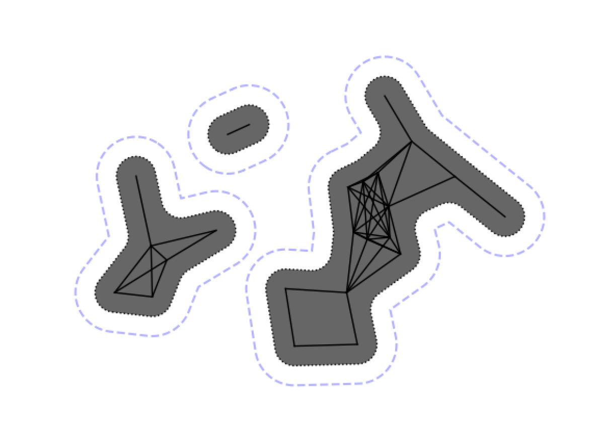
(c.2) model $F_{4}$

(d) model $F_{5}$

Figure 1. This illustrates typical realizations for the different models constructed in Examples 1.7, for which the assumptions of the qualitative homogenization result hold.

The combination of the above two lemmas shows to what extent Theorem 1.1 extends the previous literature on homogenization of the double-porosity model. In [6, 10], inclusions are indeed assumed to be both uniformly bounded and uniformly separated from one another. Many new models can now be covered, such as the following examples illustrated in Figure 1.

1. Random spherical inclusions with random radii:
   Consider a stationary ergodic random inclusion process $F_{1}=\cup_{n}I_{n}$ where the inclusions $I_{n}$’s are pairwise disjoint and where each $I_{n}$ is a ball with a random radius denoted by $r_{n}$. Consider the associated characteristic separation lengths

   $$\nu_{n}\,:=\,\tfrac{\rho_{n}}{r_{n}},\qquad\text{in terms of}\quad\rho_{n}\,:=\,\min_{m:m\neq n}\operatorname{dist}(I_{n},I_{m}),$$

   and assume that they satisfy the following moment bound, for some $\alpha>1$,

   $$\limsup_{R\uparrow\infty}\frac{1}{|B_{R}|}\sum_{n:I_{n}\cap B_{R}\neq\varnothing}\nu_{n}^{-\alpha}<\infty,\qquad\text{almost surely}.$$ (1.18)

   Qualitatively, this requires having on average more empty space around larger inclusions. By Lemmas 1.5(ii) and 1.6(i), we find that Assumption H${}_{1}(p)$ — Extension and Assumption H${}_{2}(q)$ — Elliptic regularity hold for all $p=q^{\prime}\in(1,\frac{2\alpha}{1+\alpha}]$, so Theorem 1.1 applies. For $\alpha=\infty$, the above moment bound (1.18) reduces to the uniform separation condition $\rho_{n}\geq\frac{1}{C_{0}}r_{n}$, and we then find that Assumption H${}_{1}(p)$ — Extension holds for $p=2$ without loss of integrability.

   In the special case when random radii are bounded from above and below, that is, $\inf_{n}r_{n}>0$ and $\sup_{n}r_{n}<\infty$ almost surely, then we can rather appeal to Lemma 1.5(iv): by convexity, no condition is then required on separation and we find that Assumption H${}_{1}(p)$ — Extension and Assumption H${}_{2}(q)$ — Elliptic regularity hold automatically for all $p=q^{\prime}\in(1,2\frac{d+1}{d+3})$.

2. Random cylindrical inclusions with random lengths:
   Consider a stationary ergodic random inclusion process $F_{2}=\cup_{n}I_{n}$ where the inclusions $I_{n}$’s are pairwise disjoint and where each $I_{n}$ is the isometric image of a cylinder $B^{\prime}(0,1)\times(-L_{n},L_{n})$ with unit width and random length $L_{n}\geq 1$. In this anisotropic setting, assume that the separation distances between inclusions satisfy the following moment bound, for some $\beta>1$,

   $$\limsup_{R\uparrow\infty}\frac{1}{|B_{R}|}\sum_{n:I_{n}\cap B_{R}\neq\varnothing}\Big{(}\min_{m:m\neq n}\operatorname{dist}(I_{n},I_{m})\Big{)}^{-\beta}\,<\,\infty,\qquad\text{almost surely}.$$ (1.19)

   Note that this condition is independent of the random lengths $\{L_{n}\}_{n}$, hence is much weaker than (1.18). By Lemmas 1.5(ii) and 1.6(i), we find that Assumption H${}_{1}(p)$ — Extension and Assumption H${}_{2}(q)$ — Elliptic regularity hold for all $p=q^{\prime}\in(1,\frac{2\beta}{1+\beta}]$, so Theorem 1.1 applies.

   Notably, for $\beta=\infty$, the condition (1.19) reduces to $\inf_{n\neq m}\operatorname{dist}(I_{n},I_{m})>0$ almost surely, and we then find that Assumption H${}_{1}(p)$ — Extension holds for $p=2$ without loss of integrability — which is a first to our knowledge for an inclusion process that does not satisfy the uniform separation condition (1.13).

3. Poisson inclusion processes:
   Various interesting inclusion processes can be constructed from a Poisson process $\{x_{n}\}_{n}$ on $\mathbb{R}^{d}$ and can be checked to satisfy our assumptions:

   1. Given an arbitrary stationary ergodic point process $\{x_{n}\}_{n}$ on $\mathbb{R}^{d}$, we can consider the associated inclusion process $F_{3}:=\cup_{n}I_{n}$ given by

      $$I_{n}\,:=\,B(x_{n},r_{n}),\qquad\text{with}\quad r_{n}:=\tfrac{1}{2}\min_{m:m\neq n}\operatorname{dist}(x_{n},x_{m}).$$

      By Lemmas 1.5(iv) and 1.6(i), we find that Assumption H${}_{1}(p)$ — Extension and Assumption H${}_{2}(q)$ — Elliptic regularity hold at least for all $p=q^{\prime}\in(1,2\frac{d+1}{d+3})$. Note that by definition we have $\inf_{n\neq m}\operatorname{dist}(I_{n},I_{m})=0$ almost surely and that the inclusions can be arbitrarily large or small with positive probability if $\{x_{n}\}_{n}$ is for instance a Poisson process.

   2. Given a Poisson process $\{x_{n}\}_{n}$ on $\mathbb{R}^{d}$ with intensity $\lambda$, consider the regularized clusters of unit balls around points of the process, as given e.g. by

      $$F_{4}\,:=\,\mathcal{O}\big{(}\big{\{}x\in C+2B^{\circ}\,:\,\operatorname{dist}\big{(}x,C+2B^{\circ}\big{)}>1\big{\}}\big{)},$$

      $$\text{in terms of}\quad C\,:=\,\bigcup_{n,m\atop 0<|x_{n}-x_{m}|\leq 4}[x_{n},x_{m}],$$

      where $B^{\circ}:=B(0,1)$ stands for the unit ball at the origin and where for a set $S$ we define $\mathcal{O}(S)$ to be the complement of the infinite connected component of the complement of $S$. This is well-defined and nontrivial almost surely in the subcritical Poisson percolation regime, that is, provided that the intensity of the Poisson process is small enough, $0<\lambda<\lambda_{c}$. By definition, the random set $F_{4}$ is uniformly of class $C^{2}$ and the distance between connected components is always $\geq 2$. In addition, diameters of connected components are known to have some finite exponential moments (see e.g. [15, Theorem 2]). By Lemmas 1.5(ii) and 1.6(i), we find that Assumption H${}_{1}(p)$ — Extension and Assumption H${}_{2}(q)$ — Elliptic regularity hold for all $p=q^{\prime}\in(1,2)$.

4. Subcritical percolation clusters:
   For the inclusion process $F_{5}$ in the plane $\mathbb{R}^{2}$ given by subcritical percolation clusters in random chess structure as described in Lemma 1.5(v), further applying Lemma 1.6(ii), we find that Assumption H${}_{1}(p)$ — Extension and Assumption H${}_{2}(q)$ — Elliptic regularity hold at least for all $p=q^{\prime}\in[\frac{4}{3},2)$. Note that in this setting the set $F_{5}$ is almost surely not Lipschitz due to black squares possibly touching only at a vertex. This model could be extended to higher dimensions, but we skip the details.

(a) model $F_{1}$

(b) model $F_{2}$

2. Proof of qualitative homogenization

This section is devoted to the proof of Theorem 1.1. The main technical ingredient is the following compactness result for the solution $u_{\varepsilon}$ of the double-porosity problem (1.4), which follows by combining the extension operator of Assumption Assumption H${}_{1}(p)$ — Extension together with suitable ‘resonant’ auxiliary problems inside the inclusions.

Lemma 2.1.

Let the random inclusion process $F=\cup_{n}I_{n}\subset\mathbb{R}^{d}$ satisfy Assumptions Assumption H₀, Assumption H${}_{1}(p)$ — Extension, and Assumption H${}_{2}(q)$ — Elliptic regularity for some $1<p\leq 2$ and $q=p^{\prime}$. Given a bounded Lipschitz domain $D\subset\mathbb{R}^{d}$ and $f\in{L}^{2}(D)$, for all $\varepsilon>0$, let $u_{\varepsilon}\in H^{1}_{0}(D)$ be the solution of the double-porosity problem (1.4). Then, almost surely, there exists $\bar{u}\in W^{1,p}_{0}(D)$ such that, along a subsequence, we have

$$\lim_{\varepsilon\downarrow 0}\|u_{\varepsilon}-\bar{u}\|_{{L}^{p}(D\setminus F_{\varepsilon}(D))}\,=\,0,\qquad\lim_{\varepsilon\downarrow 0}\|u_{\varepsilon}-\bar{u}-v_{\varepsilon}\|_{{L}^{p}(F_{\varepsilon}(D))}\,=\,0,$$ (2.1)

that is, in a more compact form, $\lim_{\varepsilon}\|u_{\varepsilon}-\bar{u}-\chi_{\varepsilon}v_{\varepsilon}\|_{{L}^{p}(D)}=0$, where $v_{\varepsilon}\in W^{1,p}_{0}(F_{\varepsilon}(D))$ is the solution of the auxiliary equation

$$v_{\varepsilon}-\varepsilon^{2}\triangle v_{\varepsilon}=f-\bar{u},\qquad\text{in $F_{\varepsilon}(D)$},$$ (2.2)

and where we use the same notation for $F_{\varepsilon}(D)$ and $\chi_{\varepsilon}$ as in the statement of Theorem 1.1.

Before moving on to the proof of this result, let us first note the following consequence of Assumption Assumption H${}_{2}(q)$ — Elliptic regularity. Recall that we use the short-hand notation $B^{\circ}=B(0,1)$ for the unit ball centered at the origin in $\mathbb{R}^{d}$.

Lemma 2.2.

Let the random inclusion process $F=\cup_{n}I_{n}\subset\mathbb{R}^{d}$ satisfy Assumptions Assumption H₀ and Assumption H${}_{2}(q)$ — Elliptic regularity with $q=p^{\prime}$ for some $1<p\leq 2$. Then, for all $n$ and all $f_{1}\in{L}^{p}(I_{n})$, $f_{2}\in{L}^{p}(I_{n})^{d}$, there is a unique weak solution $u\in W^{1,p}_{0}(I_{n})$ of

$$u-\triangle u=f_{1}+{\operatorname{div}}(f_{2}),\qquad\text{in $I_{n}$},$$ (2.3)

and it satisfies

$$\|u\|_{{L}^{p}(I_{n})}\,\lesssim_{\delta}\,\|f_{1}\|_{{L}^{p}(I_{n})}+\|f_{2}\|_{{L}^{p}(I_{n})},$$ (2.4)

where the multiplicative constant does not depend on $n$.

Proof of Lemma 2.2.

We focus on the proof of the estimate (2.4) in case $f_{1}\in L^{2}(I_{n})$, $f_{2}\in L^{2}(I_{n})^{d}$, while the existence part of the statement and the corresponding general estimate follow by an approximation argument. By linearity, it is enough to consider separately the cases $f_{2}=0$ and $f_{1}=0$. We split the proof into two steps accordingly.

Step 1. Case $f_{2}=0$.
Let $f_{1}\in L^{2}(I_{n})$. For any $M,\epsilon>0$, testing equation (2.3) with

$$u_{\varepsilon,M}\,:=\,\Big{(}(|u|\wedge M)^{2}+\varepsilon^{2}\Big{)}^{\frac{p-2}{2}}\Big{(}(u\wedge M)\vee(-M)\Big{)}\leavevmode\nobreak\ \in\leavevmode\nobreak\ H^{1}_{0}(I_{n}),$$

we find

$$\int_{I_{n}}\Big{(}\big{(}(|u|\wedge M)^{2}+\varepsilon^{2}\big{)}^{\frac{p-2}{2}}+(p-2)(|u|\wedge M)^{2}\big{(}(|u|\wedge M)^{2}+\varepsilon^{2}\big{)}^{\frac{p-4}{2}}\Big{)}|\nabla u|^{2}\mathds{1}_{|u|<M}\\ +\int_{I_{n}}\big{(}(|u|\wedge M)^{2}+\varepsilon^{2}\big{)}^{\frac{p-2}{2}}(|u|\wedge M)|u|\,=\,\int_{I_{n}}f_{1}u_{\varepsilon,M}.$$

Taking the limits $\varepsilon\downarrow 0$ then $M\uparrow\infty$, this entails by Hölder’s inequality

$$(p-1)\int_{I_{n}}|\nabla u|^{2}|u|^{p-2}+\int_{I_{n}}|u|^{p}=\int_{I_{n}}f_{1}u|u|^{p-2}\leq\|f_{1}\|_{{L}^{p}(I_{n})}\|{u}\|_{{L}^{p}(I_{n})}^{p-1},$$

and therefore

$$\|{u}\|_{{L}^{p}(I_{n})}\leq\|{f_{1}}\|_{{L}^{p}(I_{n})},$$

that is, (2.4).

Step 2. Case $f_{1}=0$.
We further distinguish between two cases, depending on the size of the diameter of $I_{n}$.

Substep 2.1. Case $\operatorname{diam}(I_{n})\leq 1$.
Given $h\in C^{\infty}_{c}(I_{n})^{d}$, let us consider the unique solution $z_{h}\in H^{1}_{0}(I_{n})$ of

$$z_{h}-\triangle z_{h}={\operatorname{div}}(h),\qquad\text{in $I_{n}$}.$$ (2.5)

As $\operatorname{diam}(I_{n})\leq 1$, we can choose a unit ball $B$ such that $I_{n}\subset B$. By Assumption Assumption H${}_{2}(q)$ — Elliptic regularity with $q=p^{\prime}\geq 2$, we then get

$$\|\nabla z_{h}\|_{{L}^{p^{\prime}}(I_{n})}\,\lesssim\,\|h\|_{{L}^{p^{\prime}}(I_{n})}+\|\nabla z_{h}\|_{{L}^{2}(I_{n})}.$$

By the energy estimate for $z_{h}$ and Jensen’s inequality, with $\operatorname{diam}(I_{n})\leq 1$, we can deduce

$$\|\nabla z_{h}\|_{{L}^{p^{\prime}}(I_{n})}\,\lesssim\,\|h\|_{{L}^{p^{\prime}}(I_{n})}+\|h\|_{{L}^{2}(I_{n})}\,\lesssim\,\|h\|_{{L}^{p^{\prime}}(I_{n})}.$$ (2.6)

Now for the solution $u$ of (2.3) with $f_{1}=0$, we have the duality identity

$$\int_{I_{n}}h\cdot\nabla u\,\stackrel{{\scriptstyle\eqref{e.regp66}}}{{=}}\,-\int_{I_{n}}uz_{h}-\int_{I_{n}}\nabla u\cdot\nabla z_{h}\,\stackrel{{\scriptstyle\eqref{e.regp0}}}{{=}}\,\int_{I_{n}}f_{2}\cdot\nabla z_{h},$$

which entails

$$\|\nabla u\|_{{L}^{p}(I_{n})}\,=\,\sup\Big{\{}\int_{I_{n}}h\cdot\nabla u\,:\,\|h\|_{{L}^{p^{\prime}}(I_{n})}=1\Big{\}}\,\leq\,\|f_{2}\|_{{L}^{p}(I_{n})}\sup\Big{\{}\|\nabla z_{h}\|_{{L}^{p^{\prime}}(I_{n})}\,:\,\|h\|_{{L}^{p^{\prime}}(I_{n})}=1\Big{\}},$$

and thus, by (2.6),

$$\|\nabla u\|_{{L}^{p}(I_{n})}\,\lesssim\,\|f_{2}\|_{{L}^{p}(I_{n})}.$$

By Poincaré’s inequality with $\operatorname{diam}(I_{n})\leq 1$, we may then conclude

$$\|u\|_{{L}^{p}(I_{n})}\,\lesssim\,\|\nabla u\|_{{L}^{p}(I_{n})}\,\lesssim\,\|f_{2}\|_{{L}^{p}(I_{n})},$$

that is, (2.4).

Substep 2.2. Case $\operatorname{diam}(I_{n})\geq 1$.
In this case, we need to further rely on the zeroth-order term in equation (2.3), which sets a scale in the problem. Arguing again by duality, we first claim that (2.4) is a consequence of the following: For all $f\in{L}^{p^{\prime}}(I_{n})$ with $2\leq p^{\prime}<\infty$, the solution $v_{f}\in H^{1}_{0}(I_{n})$ of

$$v_{f}-\triangle v_{f}=f,\qquad\text{in $I_{n}$},$$ (2.7)

satisfies

$$\|\nabla v_{f}\|_{{L}^{p^{\prime}}(I_{n})}\,\lesssim\,\|f\|_{{L}^{p^{\prime}}(I_{n})}.$$ (2.8)

This implication indeed follows from the duality identity

$$\int_{I_{n}}fu\,\stackrel{{\scriptstyle\eqref{e.regp4}}}{{=}}\,\int_{I_{n}}uv_{f}+\nabla u\cdot\nabla v_{f}\,\stackrel{{\scriptstyle\eqref{e.regp0}}}{{=}}\,-\int_{I_{n}}f_{2}\cdot\nabla v_{f},$$

which yields

$$\|u\|_{{L}^{p}(I_{n})}\,=\,\sup\Big{\{}\int_{I_{n}}fu\,:\,\|f\|_{{L}^{p^{\prime}}(I_{n})}=1\Big{\}}\,\leq\,\|f_{2}\|_{{L}^{p}(I_{n})}\sup\Big{\{}\|\nabla v_{f}\|_{{L}^{p^{\prime}}(I_{n})}\,:\,\|f\|_{{L}^{p^{\prime}}(I_{n})}=1\Big{\}}.$$

We now turn to the proof of (2.8), for which we proceed locally. Since ${L}^{p^{\prime}}(I_{n})\subset{L}^{2}(I_{n})$, for any unit ball $B$ with $I_{n}\cap B\neq\varnothing$, we may consider the solution $\phi_{f}\in H^{1}_{0}(2B)$ of

$$\triangle\phi_{f}=\mathds{1}_{I_{n}\cap 2B}f,\qquad\text{in $\mathbb{R}^{d}$}.$$ (2.9)

In these terms, we find $v_{f}-\triangle v_{f}={\operatorname{div}}(\nabla\phi_{f})$ in $I_{n}\cap 2B$, and Assumption Assumption H${}_{2}(q)$ — Elliptic regularity for $q=p^{\prime}$ entails

$$\|\nabla v_{f}\|_{{L}^{p^{\prime}}(I_{n}\cap B)}\,\lesssim\,\|\nabla\phi_{f}\|_{{L}^{p^{\prime}}(I_{n}\cap 2B)}+\|\nabla v_{f}\|_{{L}^{2}(I_{n}\cap 2B)}.$$

By Poincaré’s inequality in $2B$ for $\nabla\phi_{f}$, followed by the ${L}^{2}$ energy estimate for (2.9), by Calderón-Zygmund estimates in $2B$, and by Hölder’s inequality (recall $p^{\prime}\geq 2$), we get

$$\|\nabla\phi_{f}\|_{{L}^{p^{\prime}}(2B)}\,\lesssim\,\|\nabla\phi_{f}\|_{{L}^{2}(2B)}+\|\nabla^{2}\phi_{f}\|_{{L}^{p^{\prime}}(2B)}\,\lesssim\,\|f\|_{{L}^{2}(I_{n}\cap 2B)}+\|f\|_{{L}^{p^{\prime}}(I_{n}\cap 2B)}\,\lesssim\,\|f\|_{{L}^{p^{\prime}}(I_{n}\cap 2B)},$$

hence

$$\|\nabla v_{f}\|_{{L}^{p^{\prime}}(I_{n}\cap B)}\lesssim\|f\|_{{L}^{p^{\prime}}(I_{n}\cap 2B)}+\|\nabla v_{f}\|_{{L}^{2}(I_{n}\cap 2B)}.$$ (2.10)

It remains to control the second right-hand side term, and we claim that for some $M\lesssim 1$ large enough (not depending on $I_{n}$) we have the Caccioppoli-type estimate

$$\|\nabla v_{f}\|_{{L}^{2}(I_{n}\cap 2B)}\lesssim\Big{\|}e^{-\frac{|\cdot-x_{B}|}{M}}f\Big{\|}_{{L}^{p^{\prime}}(I_{n})},$$ (2.11)

where $x_{B}$ stands for the center of $B$. Before concluding the argument, let us prove this estimate. Setting $\eta:=e^{-\frac{|\cdot-x_{B}|}{M}}$, and testing (2.7) with $\eta^{2}v_{f}\in H^{1}_{0}(I_{n})$, we find

$$\int_{I_{n}}\eta^{2}v_{f}^{2}+\int_{I_{n}}\eta^{2}|\nabla v_{f}|^{2}\lesssim\int_{I_{n}}\eta^{2}|v_{f}||f|+\int_{I_{n}}\eta|v_{f}||\nabla\eta||\nabla v_{f}|,$$

which entails, for $M\lesssim 1$ large enough, by Young’s inequality and by the property $|\nabla\eta|\leq\frac{1}{M}\eta$ for the exponential,

$$\int_{I_{n}}\eta^{2}v_{f}^{2}+\int_{I_{n}}\eta^{2}|\nabla v_{f}|^{2}\lesssim\int_{I_{n}}\eta^{2}f^{2}.$$

Since $\eta\gtrsim 1$ on $I_{n}\cap 2B$, the left-hand side controls in particular $\int_{I_{n}\cap 2B}|\nabla v_{f}|^{2}$. Using Hölder’s inequality to control the right-hand side, we then get

$$\int_{I_{n}\cap 2B}|\nabla v_{f}|^{2}\,\lesssim\,\int_{I_{n}}\eta^{2}f^{2}\lesssim\,\Big{(}\int_{I_{n}}\eta^{2}\Big{)}^{1-\frac{2}{p^{\prime}}}\Big{(}\int_{I_{n}}\eta^{2}|f|^{p^{\prime}}\Big{)}^{\frac{2}{p^{\prime}}},$$

which proves (2.11).

With (2.10) and (2.11) at hand, we are now in position to conclude. For that purpose, let us cover $I_{n}$ with a finite union of unit balls $B_{i}:=B(x_{i},1)$ such that

$$\sup_{i}\sharp\left\{j\,:\,B_{i}\cap B_{j}\neq\varnothing\right\}\,\lesssim\,1.$$

Summing the contributions of the norm of $v_{f}$ in each $B_{i}$, and combining (2.10) and (2.11), we find

$$\|\nabla v_{f}\|^{p^{\prime}}_{{L}^{p^{\prime}}(I_{n})}\,\lesssim\,\sum_{i}\Big{(}\|f\|^{p^{\prime}}_{{L}^{p^{\prime}}(I_{n}\cap 2B_{i})}+\left\|e^{-\frac{|\cdot-x_{i}|}{M}}f\right\|^{p^{\prime}}_{{L}^{p^{\prime}}(I_{n})}\Big{)}\,\lesssim\,\|f\|^{p^{\prime}}_{{L}^{p^{\prime}}(I_{n})},$$

where we used that $\sum_{i}(e^{-\frac{\lvert x_{i}-\cdot\rvert}{M}}+\mathds{1}_{I_{n}\cap 2B_{i}})\lesssim 1$. This proves (2.8), hence (2.4). ∎

With the above elliptic regularity result at hand, we are now in position to prove the key compactness result of Lemma 2.1.

Proof of Lemma 2.1.

Given a ball $B$ that contains the domain $D$, and extending $u_{\varepsilon}$ by $0$ on $B\setminus D$, the extension property of Assumption Assumption H${}_{1}(p)$ — Extension allows to consider

$$\hat{u}_{\varepsilon}\,:=\,P_{B,\varepsilon}(u_{\varepsilon}\mathds{1}_{D\setminus F_{\varepsilon}(D)})|_{D}\,\in\,W^{1,p}_{0}(D),$$

which satisfies $\hat{u}_{\varepsilon}|_{D\setminus F_{\varepsilon}(D)}=u_{\varepsilon}|_{D\setminus F_{\varepsilon}(D)}$ and

$$\|\nabla\hat{u}_{\varepsilon}\|_{L^{p}(D)}\lesssim\|\nabla u_{\varepsilon}\|_{L^{2}(D\setminus F_{\varepsilon}(D))}.$$ (2.12)

By the a priori estimate for $u_{\varepsilon}$ and by Poincaré’s inequality, this entails that $\hat{u}_{\varepsilon}$ is bounded in $W^{1,p}_{0}(D)$, uniformly on the probability space. Almost surely, by Rellich’s theorem, there exists $\bar{u}\in W^{1,p}_{0}(D)$ such that $\hat{u}_{\varepsilon}\to\bar{u}$ in ${L}^{p}(D)$ along a subsequence (not relabeled). Hence, by the extension property, along this subsequence,

$$\|u_{\varepsilon}-\bar{u}\|_{{L}^{p}(D\setminus F_{\varepsilon}(D))}\,\leq\,\|\hat{u}_{\varepsilon}-\bar{u}\|_{{L}^{p}(D)}\,\xrightarrow{\varepsilon\downarrow 0}\,0.$$ (2.13)

It remains to estimate $u_{\varepsilon}-\bar{u}-v_{\varepsilon}\in W^{1,p}(F_{\varepsilon}(D))$, where $v_{\varepsilon}$ is the solution of the auxiliary problem (2.2). By the triangle inequality,

$$\|u_{\varepsilon}-\bar{u}-v_{\varepsilon}\|_{{L}^{p}(F_{\varepsilon}(D))}\leq\|u_{\varepsilon}-\hat{u}_{\varepsilon}-v_{\varepsilon}\|_{{L}^{p}(F_{\varepsilon}(D))}+\|\hat{u}_{\varepsilon}-\bar{u}\|_{{L}^{p}(D)}.$$

Since $r_{\varepsilon}:=u_{\varepsilon}-\hat{u}_{\varepsilon}-v_{\varepsilon}$ belongs to $W^{1,p}_{0}(F_{\varepsilon}(D))$ and satisfies

$$r_{\varepsilon}-\varepsilon^{2}\triangle r_{\varepsilon}=\bar{u}-\hat{u}_{\varepsilon}+\varepsilon^{2}\triangle\hat{u}_{\varepsilon},\qquad\text{in $F_{\varepsilon}(D)$},$$

Lemma 2.2 together with a rescaling argument yields

$$\|r_{\varepsilon}\|_{{L}^{p}(F_{\varepsilon}(D))}\,\lesssim\,\|\hat{u}_{\varepsilon}-\bar{u}\|_{{L}^{p}(D)}+\varepsilon\|\nabla\hat{u}_{\varepsilon}\|_{{L}^{p}(D)}.$$

Combined with (2.12) and (2.13), this concludes the proof. ∎

Combining the extension property of Assumption Assumption H${}_{1}(p)$ — Extension together with the compactness result of Lemma 2.1, we can control the solution inside inclusions by its value outside, and we may then proceed to the proof of Theorem 1.1 with Tartar’s method of oscillating test functions. In order to accommodate the mere ${L}^{p}$ control inside inclusions given by Lemma 2.1, we use approximate correctors in Tartar’s argument, as well as a truncation argument. The use of approximate correctors raises some interesting subtleties, and we have to unravel some hidden monotonicity to conclude.

Proof of Theorem 1.1.

Recall the a priori estimates for $u_{\varepsilon}$,

$$\|u_{\varepsilon}\|_{{L}^{2}(D)}\lesssim 1,\qquad\|(1-\chi_{\varepsilon}+\varepsilon\chi_{\varepsilon})\nabla u_{\varepsilon}\|_{{L}^{2}(D)}\lesssim 1.$$

Appealing to Lemma 2.1, for a given typical realization, there exists $\bar{u}\in W^{1,p}_{0}(D)$ such that, along a subsequence (not relabeled), we have

$$\|u_{\varepsilon}-\bar{u}\|_{{L}^{p}(D\setminus F_{\varepsilon}(D))}\to 0,\qquad\|u_{\varepsilon}-\bar{u}-v_{\varepsilon}\|_{{L}^{p}(F_{\varepsilon}(D))}\to 0,$$ (2.14)

where $v_{\varepsilon}$ is defined in Lemma 2.1. Note that at this stage we do not know yet that $\bar{u}$ satisfies an equation, nor even that $\bar{u}\in H^{1}_{0}(D)$ since $1<p\leq 2$. This will only be deduced at the end of the proof. We split the proof into four main steps.

Step 1. Approximate corrector.
For $\varepsilon>0$ and $1\leq i\leq d$, we define $\varphi_{\varepsilon i}\in H^{1}_{\operatorname{loc}}(\mathbb{R}^{d};{L}^{2}(\Omega))$ as the unique stationary weak solution of

$$\varepsilon\varphi_{\varepsilon i}-\nabla\cdot(\mathds{1}_{\mathbb{R}^{d}\setminus F}+\varepsilon^{2}\mathds{1}_{F})(e_{i}+\nabla\varphi_{\varepsilon i})=0,\qquad\text{in $\mathbb{R}^{d}$},$$ (2.15)

and we then set $\varphi_{\varepsilon}:=\{\varphi_{\varepsilon i}\}_{1\leq i\leq d}$. We emphasize that the existence of a stationary solution $\varphi_{\varepsilon i}$ to the above equation is ensured by uniqueness thanks to the massive term. We show that this approximate corrector $\varphi_{\varepsilon}$ satisfies the following five properties:

1. $\mathbb{E}[\mathds{1}_{\mathbb{R}^{d}\setminus F}|\nabla\varphi_{\varepsilon}-\nabla\varphi|^{2}]\to 0$ as $\varepsilon\downarrow 0$;

2. $\varepsilon\mathbb{E}[|\varphi_{\varepsilon}|^{2}]\to 0$ as $\varepsilon\downarrow 0$;

3. $\varepsilon^{2}\mathbb{E}[\mathds{1}_{F}|\nabla\varphi_{\varepsilon}|^{2}]\to 0$ as $\varepsilon\downarrow 0$;

4. $\sup_{x\in\mathbb{R}^{d}}\fint_{B(x,\varepsilon^{-1/2})}\varepsilon|\varphi_{\varepsilon}|^{2}\lesssim 1$;

5. $\sup_{x\in\mathbb{R}^{d}}\fint_{B(x,\varepsilon^{-1/2})}(\mathds{1}_{\mathbb{R}^{d}\setminus F}+\varepsilon^{2}\mathds{1}_{F})|\nabla\varphi_{\varepsilon}|^{2}\lesssim 1$.

We split the proof of (i)–(v) into three further substeps.

Substep 1.1. Proof of a weak version of (i): for all $1\leq i\leq d$, we have the weak convergence

$$\mathds{1}_{\mathbb{R}^{d}\setminus F}\nabla\varphi_{\varepsilon}\rightharpoonup\mathds{1}_{\mathbb{R}^{d}\setminus F}\nabla\varphi,\qquad\text{in ${L}^{2}(\Omega)$.}$$ (2.16)

Let $1\leq i\leq d$ be fixed. First note the following a priori estimate for $\varphi_{\varepsilon i}$,

$$\varepsilon\mathbb{E}[|\varphi_{\varepsilon i}|^{2}]+\varepsilon^{2}\mathbb{E}[\mathds{1}_{F}|\nabla\varphi_{\varepsilon i}|^{2}]+\mathbb{E}[\mathds{1}_{\mathbb{R}^{d}\setminus F}|\nabla\varphi_{\varepsilon i}|^{2}]\,\lesssim\,1.$$ (2.17)

By Assumption Assumption H${}_{1}(p)$ — Extension, as $\mathds{1}_{\mathbb{R}^{d}\setminus F}\nabla\varphi_{\varepsilon i}$ is bounded in ${L}^{2}(\Omega)$, we can construct a stationary field $\hat{\varphi}_{\varepsilon i}:=P\varphi_{\varepsilon i}\in W^{1,p}_{\operatorname{loc}}(\mathbb{R}^{d};{L}^{p}(\Omega))$ such that $\hat{\varphi}_{\varepsilon i}=\varphi_{\varepsilon i}$ in $\mathbb{R}^{d}\setminus F$ and such that $\nabla\hat{\varphi}_{\varepsilon i}$ is bounded in ${L}^{p}(\Omega)$. Hence, by weak compactness, there is a stationary potential random field $\Phi_{i}\in{L}^{p}(\Omega)$ with $\mathbb{E}[\Phi_{i}]=0$ such that $\nabla\hat{\varphi}_{\varepsilon i}\rightharpoonup\Phi_{i}$ in ${L}^{p}(\Omega)$. By the definition of the extension, this implies $\mathds{1}_{\mathbb{R}^{d}\setminus F}\nabla\varphi_{\varepsilon i}=\mathds{1}_{\mathbb{R}^{d}\setminus F}\nabla\hat{\varphi}_{\varepsilon i}\rightharpoonup\mathds{1}_{\mathbb{R}^{d}\setminus F}\Phi_{i}$ in ${L}^{p}(\Omega)$. By the boundedness of $\mathds{1}_{\mathbb{R}^{d}\setminus F}\nabla\varphi_{\varepsilon i}$ in ${L}^{2}(\Omega)$, this weak convergence must actually hold in ${L}^{2}(\Omega)$. Testing the corrector equation (2.15) for $\varphi_{\varepsilon i}$ with some stationary field $\psi\in{L}^{2}(\Omega;H^{1}_{\operatorname{loc}}(\mathbb{R}^{d}))$, passing to the limit $\varepsilon\downarrow 0$, and using the a priori estimates (2.17), we get

$$\mathbb{E}\left[\nabla\psi\cdot(\Phi_{i}+e_{i})\mathds{1}_{\mathbb{R}^{d}\setminus F}\right]=0,$$

and therefore, by density, for all stationary potential random fields $\Psi\in{L}^{2}(\Omega)$ with $\mathbb{E}[\Psi]=0$,

$$\mathbb{E}\left[\Psi\cdot(\Phi_{i}+e_{i})\mathds{1}_{\mathbb{R}^{d}\setminus F}\right]=0.$$

As this is the weak formulation of equation (1.8) in the probability space, we conclude $\mathds{1}_{\mathbb{R}^{d}\setminus F}\Phi_{i}=\mathds{1}_{\mathbb{R}^{d}\setminus F}\nabla\varphi_{i}$, and this proves the claimed weak convergence (2.16).

Substep 1.2. Proof of (i)–(iii).
We appeal to an energy argument. From the equations for $\varphi_{\varepsilon i}$ and $\varphi_{i}$, we find respectively

$$\varepsilon\mathbb{E}[|\varphi_{\varepsilon i}|^{2}]+\varepsilon^{2}\mathbb{E}[\mathds{1}_{F}|\nabla\varphi_{\varepsilon i}|^{2}]+\mathbb{E}[\mathds{1}_{\mathbb{R}^{d}\setminus F}|\nabla\varphi_{\varepsilon i}|^{2}] = -e_{i}\cdot\mathbb{E}[\mathds{1}_{\mathbb{R}^{d}\setminus F}\nabla\varphi_{\varepsilon i}]-\varepsilon^{2}e_{i}\cdot\mathbb{E}[\mathds{1}_{F}\nabla\varphi_{\varepsilon i}],$$

$$\mathbb{E}[\mathds{1}_{\mathbb{R}^{d}\setminus F}|\nabla\varphi_{i}|^{2}] = -e_{i}\cdot\mathbb{E}[\mathds{1}_{\mathbb{R}^{d}\setminus F}\nabla\varphi_{i}],$$

and thus,

$$\varepsilon\mathbb{E}[|\varphi_{\varepsilon i}|^{2}]+\varepsilon^{2}\mathbb{E}[\mathds{1}_{F}|\nabla\varphi_{\varepsilon i}|^{2}]+\mathbb{E}[\mathds{1}_{\mathbb{R}^{d}\setminus F}|\nabla\varphi_{\varepsilon i}-\nabla\varphi_{i}|^{2}]\\ \,=\,-\mathbb{E}[\mathds{1}_{\mathbb{R}^{d}\setminus F}(2\nabla\varphi_{i}+e_{i})\cdot(\nabla\varphi_{\varepsilon i}-\nabla\varphi_{i})]-\varepsilon^{2}e_{i}\cdot\mathbb{E}[\mathds{1}_{F}\nabla\varphi_{\varepsilon i}].$$

From the weak convergence established in Step 1.1, we can pass to the limit in the right-hand side and conclude

$$\lim_{\varepsilon\downarrow 0}\Big{(}\varepsilon\mathbb{E}[|\varphi_{\varepsilon}|^{2}]+\varepsilon^{2}\mathbb{E}[\mathds{1}_{F}|\nabla\varphi_{\varepsilon}|^{2}]+\mathbb{E}[\mathds{1}_{\mathbb{R}^{d}\setminus F}|\nabla\varphi_{\varepsilon}-\nabla\varphi|^{2}]\Big{)}\,=\,0,$$

which proves items (i)–(iii).

Substep 1.3. Proof of (iv)–(v).
We appeal to Caccioppoli’s inequality. In terms of the exponential cutoff $\eta_{x}(y):=\exp(-\frac{1}{2}\sqrt{\varepsilon}|y-x|)$, let us test the approximate corrector equation (2.15) with $\eta_{x}^{2}\varphi_{\varepsilon i}$. With the short-hand notation $\alpha_{\varepsilon}:=\mathds{1}_{\mathbb{R}^{d}\setminus F}+\varepsilon^{2}\mathds{1}_{F}$, this yields

$$\int_{\mathbb{R}^{d}}\eta_{x}^{2}\varepsilon\varphi_{\varepsilon i}^{2}+\int_{\mathbb{R}^{d}}\alpha_{\varepsilon}\eta_{x}^{2}|\nabla\varphi_{\varepsilon i}|^{2}\,=\,-2e_{i}\cdot\int_{\mathbb{R}^{d}}\alpha_{\varepsilon}\varphi_{\varepsilon i}\eta_{x}\nabla\eta_{x}-e_{i}\cdot\int_{\mathbb{R}^{d}}\alpha_{\varepsilon}\eta_{x}^{2}\nabla\varphi_{\varepsilon i}-2\int_{\mathbb{R}^{d}}\alpha_{\varepsilon}\eta_{x}\varphi_{\varepsilon i}\nabla\eta_{x}\cdot\nabla\varphi_{\varepsilon i}.$$

Using $|\nabla\eta_{x}|\leq\frac{1}{2}\sqrt{\varepsilon}\eta_{x}$ and Young’s inequality to absorb the last right-hand side term, we are led to

$$\int_{\mathbb{R}^{d}}\eta_{x}^{2}\varepsilon\varphi_{\varepsilon i}^{2}+\int_{\mathbb{R}^{d}}\alpha_{\varepsilon}\eta_{x}^{2}|\nabla\varphi_{\varepsilon i}|^{2}\,\lesssim\,\int_{\mathbb{R}^{d}}\eta_{x}^{2}(\sqrt{\varepsilon}|\varphi_{\varepsilon i}|+\alpha_{\varepsilon}|\nabla\varphi_{\varepsilon i}|),$$

and thus, by the Cauchy–Schwarz inequality,

$$\int_{\mathbb{R}^{d}}\eta_{x}^{2}\varepsilon\varphi_{\varepsilon i}^{2}+\int_{\mathbb{R}^{d}}\alpha_{\varepsilon}\eta_{x}^{2}|\nabla\varphi_{\varepsilon i}|^{2}\,\lesssim\,\int_{\mathbb{R}^{d}}\eta_{x}^{2}\,\lesssim\,\varepsilon^{-\frac{d}{2}}.$$

As $\eta_{x}^{2}|_{B(x,\varepsilon^{-1/2})}\gtrsim 1$, this concludes the proof of items (iv) and (v).

Step 2. Oscillating test-functions.
Given $\psi\in C^{\infty}_{c}(D)$, testing the equation for $u_{\varepsilon}$ with $\psi+\varepsilon\varphi_{\varepsilon i}(\tfrac{\cdot}{\varepsilon})\nabla_{i}\psi$, we obtain

$$\int_{D}u_{\varepsilon}(\psi+\varepsilon\varphi_{\varepsilon i}(\tfrac{\cdot}{\varepsilon})\nabla_{i}\psi)+\int_{D}(\nabla_{i}\psi)(e_{i}+\nabla\varphi_{\varepsilon i}(\tfrac{\cdot}{\varepsilon}))\cdot(1-\chi_{\varepsilon}+\varepsilon^{2}\chi_{\varepsilon})\nabla u_{\varepsilon}\\ +\int_{D}\varepsilon\varphi_{\varepsilon i}(\tfrac{\cdot}{\varepsilon})(\nabla\nabla_{i}\psi)\cdot(1-\chi_{\varepsilon}+\varepsilon^{2}\chi_{\varepsilon})\nabla u_{\varepsilon}=\int_{D}f(\psi+\varepsilon\varphi_{\varepsilon i}(\tfrac{\cdot}{\varepsilon})\nabla_{i}\psi).$$

Integrating by parts in the second term, using the corrector equation, and noting that $\chi_{\varepsilon}=\mathds{1}_{\varepsilon F}$ on the support of $\psi$ for $\varepsilon$ small enough, this entails

$$\int_{D}u_{\varepsilon}\psi-\int_{D}u_{\varepsilon}(1-\chi_{\varepsilon}+\varepsilon^{2}\chi_{\varepsilon})(e_{i}+\nabla\varphi_{\varepsilon i}(\tfrac{\cdot}{\varepsilon}))\cdot(\nabla\nabla_{i}\psi)\\ +\int_{D}\varepsilon\varphi_{\varepsilon i}(\tfrac{\cdot}{\varepsilon})(\nabla\nabla_{i}\psi)\cdot(1-\chi_{\varepsilon}+\varepsilon^{2}\chi_{\varepsilon})\nabla u_{\varepsilon}=\int_{D}f(\psi+\varepsilon\varphi_{\varepsilon i}(\tfrac{\cdot}{\varepsilon})\nabla_{i}\psi).$$

By the Cauchy–Schwarz inequality and by the uniform bounds (iv)–(v) of Step 1 on $\varphi_{\varepsilon}$ and $\nabla\varphi_{\varepsilon}$ averaged over balls of radius $\varepsilon^{-1/2}$, this yields in the limit $\varepsilon\downarrow 0$,

$$\lim_{\varepsilon\downarrow 0}\Big{(}\int_{D}u_{\varepsilon}\psi-\int_{D}u_{\varepsilon}(1-\chi_{\varepsilon})(e_{i}+\nabla\varphi_{\varepsilon i}(\tfrac{\cdot}{\varepsilon}))\cdot(\nabla\nabla_{i}\psi)\Big{)}=\int_{D}f\psi,$$ (2.18)

and it remains to pass to the limit in both left-hand side terms.

Step 3. Conclusion.
By (2.14) in form of $\|u_{\varepsilon}-\bar{u}-\chi_{\varepsilon}v_{\varepsilon}\|_{L^{p}(D)}\to 0$ and by the ergodic theorem on $v_{\varepsilon}$, we find for the first summand in (2.18),

$$\lim_{\varepsilon\downarrow 0}\int_{D}u_{\varepsilon}\psi\,=\,\mathbb{E}[v]\int_{D}(f-\bar{u})\psi+\int_{D}\bar{u}\psi.$$

Let us now turn to the second summand in (2.18) and assume for now that one can replace $\nabla\varphi_{\varepsilon i}$ by $\nabla\varphi_{i}$ in that term — which we shall indeed prove in Step 4 below. We appeal to a truncation argument and set $u_{\varepsilon,N}:=(u_{\varepsilon}\vee(-N))\wedge N$ for $N\geq 1$. The strong convergence (2.14) in ${L}^{p}(D)$ entails that, along a subsequence (not relabeled), there exists a Lebesgue-negligible set $Z\subset D$ such that

$$|u_{\varepsilon}(x)-\bar{u}(x)-\chi_{\varepsilon}(x)v_{\varepsilon}(x)|\xrightarrow{\varepsilon\downarrow 0}0,\qquad\text{for all }x\in D\setminus Z.$$

Egorov’s theorem entails in turn that, for fixed $N\geq 1$, there exists $Z\subset Z_{N}\subset D$ such that $\left\lvert Z_{N}\right\rvert\leq 2^{-N}$ and there exists $\varepsilon(N)>0$ such that

$$|u_{\varepsilon}(x)-\bar{u}(x)-\chi_{\varepsilon}(x)v_{\varepsilon}(x)|\,\leq\,\tfrac{N}{2},\qquad\text{for all $x\in D\setminus Z_{N}$ and all $0<\varepsilon<\varepsilon(N)$.}$$

Hence, by the triangle inequality, for all $x\in D\setminus Z_{N}$ and all $0<\varepsilon<\varepsilon(N)$,

$$(1-\chi_{\varepsilon}(x))\mathds{1}_{|u_{\varepsilon}(x)|\geq N}\,\leq\,\mathds{1}_{|\bar{u}(x)|\geq\frac{N}{2}}.$$ (2.19)

In particular, by the Cauchy–Schwarz inequality, by (2.19), and by the a priori estimate for $u_{\varepsilon}$ in $L^{2}(D)$,

$$\bigg{|}\int_{D}u_{\varepsilon}(1-\chi_{\varepsilon})(e_{i}+\nabla\varphi_{i}(\tfrac{\cdot}{\varepsilon}))\cdot(\nabla\nabla_{i}\psi)-\int_{D}u_{\varepsilon,N}(1-\chi_{\varepsilon})(e_{i}+\nabla\varphi_{i}(\tfrac{\cdot}{\varepsilon}))\cdot(\nabla\nabla_{i}\psi)\bigg{|}\\ \,\lesssim\,\Big{(}\int_{D}|u_{\varepsilon}|^{2}\Big{)}^{\frac{1}{2}}\Big{(}\int_{D}(1-\chi_{\varepsilon})\mathds{1}_{|u_{\varepsilon}|\geq N}|e_{i}+\nabla\varphi_{i}(\tfrac{\cdot}{\varepsilon})|^{2}\Big{)}^{\frac{1}{2}}\,\lesssim\,\Big{(}\int_{D}\big{(}\mathds{1}_{Z_{N}}+\mathds{1}_{|\bar{u}|\geq\frac{N}{2}}\big{)}|e_{i}+\nabla\varphi_{i}(\tfrac{\cdot}{\varepsilon})|^{2}\Big{)}^{\frac{1}{2}}.$$

Now using the ergodic theorem to pass to the limit $\varepsilon\downarrow 0$ and then using the monotone convergence theorem to pass to the limit $N\uparrow\infty$, we find

$$\limsup_{N\uparrow\infty}\limsup_{\varepsilon\downarrow 0}\bigg{|}\int_{D}u_{\varepsilon}(1-\chi_{\varepsilon})(e_{i}+\nabla\varphi_{i}(\tfrac{\cdot}{\varepsilon}))\cdot(\nabla\nabla_{i}\psi)-\int_{D}u_{\varepsilon,N}(1-\chi_{\varepsilon})(e_{i}+\nabla\varphi_{i}(\tfrac{\cdot}{\varepsilon}))\cdot(\nabla\nabla_{i}\psi)\bigg{|}\\ \,\lesssim\,\mathbb{E}\big{[}|e_{i}+\nabla\varphi_{i}|^{2}\big{]}^{\frac{1}{2}}\lim_{N\uparrow\infty}\Big{(}2^{-N}+\int_{D}\mathds{1}_{|\bar{u}|\geq\frac{N}{2}}\Big{)}^{\frac{1}{2}}\,=\,0.$$

Note that for fixed $N$ it follows from (2.14) that $(1-\chi_{\varepsilon})(u_{\varepsilon,N}-\bar{u}_{N})\to 0$ in ${L}^{2}(D)$ as $\varepsilon\downarrow 0$, where we have similarly defined $\bar{u}_{N}:=(\bar{u}\vee(-N))\wedge N$. Further using the ergodic theorem and the definition of $\bar{a}$, cf. (1.9), we may then infer

$$\lim_{N\uparrow\infty}\limsup_{\varepsilon\downarrow 0}\bigg{|}\int_{D}u_{\varepsilon}(1-\chi_{\varepsilon})(e_{i}+\nabla\varphi_{i}(\tfrac{\cdot}{\varepsilon}))\cdot(\nabla\nabla_{i}\psi)-\int_{D}\bar{u}_{N}e_{i}\cdot\bar{a}(\nabla\nabla_{i}\psi)\bigg{|}\,=\,0.$$

Passing to the limit $N\uparrow\infty$ in $\bar{u}_{N}$ and integrating by parts, we conclude

$$\lim_{\varepsilon\downarrow 0}\int_{D}u_{\varepsilon}(1-\chi_{\varepsilon})(e_{i}+\nabla\varphi_{i}(\tfrac{\cdot}{\varepsilon}))\cdot(\nabla\nabla_{i}\psi)\,=\,-\int_{D}\nabla\bar{u}\cdot\bar{a}\nabla\psi.$$

Inserting these different limits into (2.18), and assuming that the approximate corrector $\nabla\varphi_{\varepsilon i}$ could be replaced by $\nabla\varphi_{i}$ in (2.18), we would conclude

$$(1-\mathbb{E}[v])\int_{D}\bar{u}\psi+\int_{D}\nabla\bar{u}\cdot\bar{a}\nabla\psi=(1-\mathbb{E}[v])\int_{D}f\psi,$$

meaning that $\bar{u}$ satisfies the claimed homogenized problem (1.6). By [25, Lemma 8.8], the extension property of Assumption Assumption H${}_{1}(p)$ — Extension together with the assumption $\mathbb{E}[\mathds{1}_{F}]<1$ implies that $\bar{a}$ is positive definite, so that $\bar{u}$ is uniquely defined as the solution of the homogenized problem and belongs to $H^{1}_{0}(D)$. This allows to get rid of the extractions, which concludes the proof.

Step 4. Replacing $\nabla\varphi_{\varepsilon}$ by $\nabla\varphi$ in (2.18).
Since $\psi$ is compactly supported in $D$ and since we have $\chi_{\varepsilon}=\mathds{1}_{\varepsilon F}$ in the support of $\psi$ for $\varepsilon$ small enough, it suffices to prove that on any ball $B\subset\mathbb{R}^{d}$ we have almost surely

$$\lim_{\varepsilon\downarrow 0}\int_{B}\mathds{1}_{\mathbb{R}^{d}\setminus\varepsilon F}|\nabla\varphi_{\varepsilon}(\tfrac{\cdot}{\varepsilon})-\nabla\varphi(\tfrac{\cdot}{\varepsilon})|^{2}\,=\,0.$$ (2.20)

This convergence is not a simple consequence of Step 1. Indeed, in Step 1, we only showed the convergence of the expectation $\mathbb{E}[\mathds{1}_{\mathbb{R}^{d}\setminus F}|\nabla\varphi_{\varepsilon}-\nabla\varphi|^{2}]\to 0$ as $\varepsilon\downarrow 0$. In order to actually go from the almost sure quantity to its expectation, one would first need to appeal to the ergodic theorem for large-scale averages as $\varepsilon\downarrow 0$. This amounts to considering a diagonal limit in both convergences, which is especially delicate since we are deprived of any quantitative statement. Instead we shall use some hidden monotonicity.

Without loss of generality, let us focus on correctors in the direction $e_{1}$. In order to prove (2.20), we then claim that it is enough to show that for all radially-symmetric smooth compactly supported functions $\eta:\mathbb{R}^{d}\to[0,1]$ we have almost surely

$$\lim_{\varepsilon\downarrow 0}\int_{\mathbb{R}^{d}}\eta\mathds{1}_{\mathbb{R}^{d}\setminus\varepsilon F}|e_{1}+\nabla\varphi_{\varepsilon 1}(\tfrac{\cdot}{\varepsilon})|^{2}\,=\,\Big{(}\int_{\mathbb{R}^{d}}\eta\Big{)}\,\mathbb{E}\left[\mathds{1}_{\mathbb{R}^{d}\setminus F}|e_{1}+\nabla\varphi_{1}|^{2}\right].$$ (2.21)

Indeed, setting for abbreviation $\eta_{\varepsilon}:=\eta(\varepsilon\cdot)$, and rescaling and expanding the square, we find

$$\int_{\mathbb{R}^{d}}\eta\mathds{1}_{\mathbb{R}^{d}\setminus\varepsilon F}|\nabla\varphi_{\varepsilon 1}(\tfrac{\cdot}{\varepsilon})-\nabla\varphi_{1}(\tfrac{\cdot}{\varepsilon})|^{2}$$

$$= \varepsilon^{d}\int_{\mathbb{R}^{d}}\eta_{\varepsilon}\mathds{1}_{\mathbb{R}^{d}\setminus F}(|e_{1}+\nabla\varphi_{1}|^{2}+|e_{1}+\nabla\varphi_{\varepsilon 1}|^{2})-2\varepsilon^{d}\int_{\mathbb{R}^{d}}\eta_{\varepsilon}\mathds{1}_{\mathbb{R}^{d}\setminus F}(e_{1}+\nabla\varphi_{\varepsilon 1})\cdot(e_{1}+\nabla\varphi_{1})$$

$$= \varepsilon^{d}\int_{\mathbb{R}^{d}}\eta_{\varepsilon}\mathds{1}_{\mathbb{R}^{d}\setminus F}(|e_{1}+\nabla\varphi_{1}|^{2}+|e_{1}+\nabla\varphi_{\varepsilon 1}|^{2})-2\varepsilon^{d}\int_{\mathbb{R}^{d}}\eta_{\varepsilon}\mathds{1}_{\mathbb{R}^{d}\setminus F}e_{1}\cdot(e_{1}+\nabla\varphi_{1})$$

$$\hskip 28.45274pt-2\varepsilon^{d}\int_{\mathbb{R}^{d}}\eta_{\varepsilon}\mathds{1}_{\mathbb{R}^{d}\setminus F}\nabla\varphi_{\varepsilon 1}\cdot(e_{1}+\nabla\varphi_{1}).$$

First, note that the last right-hand side term vanishes as $\varepsilon\downarrow 0$. Indeed, integrating by parts and using the corrector equation (1.8), it can be written as

$$\varepsilon^{d}\int_{\mathbb{R}^{d}}\eta_{\varepsilon}\mathds{1}_{\mathbb{R}^{d}\setminus F}\nabla\varphi_{\varepsilon 1}\cdot(e_{1}+\nabla\varphi_{1})\,=\,-\varepsilon^{d}\int_{\mathbb{R}^{d}}\varepsilon\varphi_{\varepsilon 1}\mathds{1}_{\mathbb{R}^{d}\setminus F}(\nabla\eta)(\varepsilon\cdot)\cdot(e_{1}+\nabla\varphi_{1}).$$

By the ergodic theorem in form of $\varepsilon^{d}\int_{K}\mathds{1}_{\mathbb{R}^{d}\setminus F}|e_{1}+\nabla\varphi_{1}|^{2}\to|K|\,\mathbb{E}[\mathds{1}_{\mathbb{R}^{d}\setminus F}|e_{1}+\nabla\varphi_{1}|^{2}]<\infty$ on any compact set $K\subset\mathbb{R}^{d}$, together with the bounds on averages of $\varphi_{\varepsilon 1}$ in Step 1, we deduce

$$\lim_{\varepsilon\downarrow 0}\varepsilon^{d}\int_{\mathbb{R}^{d}}\eta_{\varepsilon}\mathds{1}_{\mathbb{R}^{d}\setminus F}\nabla\varphi_{\varepsilon 1}\cdot(e_{1}+\nabla\varphi_{1})\,=\,0.$$

Further noting that the ergodic theorem and the corrector equation (1.8) yield

$$\lim_{\varepsilon\downarrow 0}\bigg{(}\varepsilon^{d}\int_{\mathbb{R}^{d}}\eta_{\varepsilon}\mathds{1}_{\mathbb{R}^{d}\setminus F}|e_{1}+\nabla\varphi_{1}|^{2}-2\varepsilon^{d}\int_{\mathbb{R}^{d}}\eta_{\varepsilon}\mathds{1}_{\mathbb{R}^{d}\setminus F}e_{1}\cdot(e_{1}+\nabla\varphi_{1})\bigg{)}\\ \,=\,\Big{(}\int_{\mathbb{R}^{d}}\eta\Big{)}\mathbb{E}\Big{[}\mathds{1}_{\mathbb{R}^{d}\setminus F}|e_{1}+\nabla\varphi_{1}|^{2}-2\mathds{1}_{\mathbb{R}^{d}\setminus F}e_{1}\cdot(e_{1}+\nabla\varphi_{1})\Big{]}\,=\,-\Big{(}\int_{\mathbb{R}^{d}}\eta\Big{)}\mathbb{E}\Big{[}\mathds{1}_{\mathbb{R}^{d}\setminus F}|e_{1}+\nabla\varphi_{1}|^{2}\Big{]},$$

the above becomes

$$\lim_{\varepsilon\downarrow 0}\bigg{(}\int_{\mathbb{R}^{d}}\eta\mathds{1}_{\mathbb{R}^{d}\setminus\varepsilon F}|\nabla\varphi_{1}(\tfrac{\cdot}{\varepsilon})-\nabla\varphi_{\varepsilon 1}(\tfrac{\cdot}{\varepsilon})|^{2}-\varepsilon^{d}\int_{\mathbb{R}^{d}}\eta_{\varepsilon}\mathds{1}_{\mathbb{R}^{d}\setminus F}|e_{1}+\nabla\varphi_{\varepsilon 1}|^{2}+\Big{(}\int_{\mathbb{R}^{d}}\eta\Big{)}\mathbb{E}\Big{[}\mathds{1}_{\mathbb{R}^{d}\setminus F}|e_{1}+\nabla\varphi_{1}|^{2}\Big{]}\bigg{)}=0,$$

meaning that (2.20) for correctors in the direction $e_{1}$ is indeed equivalent to (2.21).

It remains to prove (2.21), which we shall actually establish in the following slightly modified form: For all balls $B$, we have almost surely

$$\lim_{\varepsilon\downarrow 0}\fint_{B}\mathds{1}_{\mathbb{R}^{d}\setminus\varepsilon F}|e_{1}+\nabla\varphi_{\varepsilon 1}(\tfrac{\cdot}{\varepsilon})|^{2}\,=\,\mathbb{E}\left[\mathds{1}_{\mathbb{R}^{d}\setminus F}|e_{1}+\nabla\varphi_{1}|^{2}\right].$$ (2.22)

Let us briefly argue that this indeed implies (2.21). Let $\eta:\mathbb{R}^{d}\to[0,1]$ be a radially-symmetric smooth function supported in a ball $B(0,R)$. Since for any integrable function $g$ we have

$$\int_{B(0,R)}\eta g\,=\,\int_{0}^{R}\eta(r)\Big{(}\int_{\partial B(0,r)}g\Big{)}dr\,=\,-\int_{0}^{R}\eta^{\prime}(r)\Big{(}\int_{B(0,r)}g\Big{)}dr,$$

the claim (2.21) follows from integrating (2.22) for $B=B(0,r)$ over $r\in(0,R)$, and appealing to dominated convergence together with the uniform bound (v) of Step 1 on averages of $\nabla\varphi_{\varepsilon 1}$.

We are left with proving (2.22), and we split the argument into four further substeps, relying on the subadditive ergodic theorem.

Substep 4.1. Application of the subadditive ergodic theorem.
Consider the random set function $\mathcal{F}$ given for all bounded open sets $O\subset\mathbb{R}^{d}$ by

$$\mathcal{F}(O)\,:=\,\inf_{\psi\in H^{1}_{0}(O)}\int_{O}\Big{(}\tfrac{2}{d_{O}}\psi^{2}+(\mathds{1}_{\mathbb{R}^{d}\setminus F}+\tfrac{4}{d_{O}^{2}}\mathds{1}_{F})|e_{1}+\nabla\psi|^{2}\Big{)},$$

where $d_{O}:=\operatorname{diam}(O)$. This is a rather unusual form for an integral functional since the integrand depends itself on the set. Since $F$ is stationary, $\mathcal{F}$ is also stationary. So defined, the set function $\mathcal{F}$ is subadditive in the sense that for all disjoint bounded open sets $O_{1},\dots,O_{N}$ we have

$$\mathcal{F}(\cup_{i=1}^{N}O_{i})\leq\sum_{i=1}^{N}\mathcal{F}(O_{i}),$$

which indeed follows from the gluing properties of Dirichlet conditions and from $d_{\cup_{i=1}^{N}O_{i}}\geq\max_{1\leq i\leq N}d_{O_{i}}$. In addition, note that

$$\mathcal{F}(O)\leq|O|(1\vee\tfrac{1}{d_{0}^{2}}).$$

In this setting, the subadditive ergodic theorem entails that there exists some $\bar{\mathcal{F}}\geq 0$ such that almost surely we have for all bounded open sets $O\subset\mathbb{R}^{d}$,

$$\lim_{R\uparrow\infty}|RO|^{-1}\mathcal{F}(RO)\,=\,\lim_{R\uparrow\infty}\mathbb{E}\left[|RO|^{-1}\mathcal{F}(RO)\right]\,=\,\bar{\mathcal{F}}.$$ (2.23)

Substep 4.2. Link to approximate corrector: for any unit ball $B\subset\mathbb{R}^{d}$ and any $\varepsilon>0$ we have almost surely

$$|B/\varepsilon|^{-1}\mathcal{F}(B/\varepsilon)-C\varepsilon^{\frac{1}{2}}\,\leq\,\fint_{B/\varepsilon}\Big{(}\varepsilon\varphi_{\varepsilon 1}^{2}+(\mathds{1}_{\mathbb{R}^{d}\setminus F}+\varepsilon^{2}\mathds{1}_{F})|e_{1}+\nabla\varphi_{\varepsilon 1}|^{2}\Big{)}\,\leq\,|B/\varepsilon|^{-1}\mathcal{F}(B/\varepsilon)+C\varepsilon^{\frac{1}{2}},$$ (2.24)

from which we shall deduce in particular that the limit $\bar{\mathcal{F}}$ in (2.23) is equal to

$$\bar{\mathcal{F}}\,=\,\mathbb{E}\left[\mathds{1}_{\mathbb{R}^{d}\setminus F}|e_{1}+\nabla\varphi_{1}|^{2}\right]\,=\,e_{1}\cdot\bar{a}e_{1}.$$ (2.25)

We start with the proof of (2.24). Let $B\subset\mathbb{R}^{d}$ be a unit ball and let $\varepsilon>0$. As $\operatorname{diam}(B/\varepsilon)=\frac{2}{\varepsilon}$, the definition of $\mathcal{F}$ reads

$$\mathcal{F}(B/\varepsilon)\,=\,\inf_{\psi\in H^{1}_{0}(B/\varepsilon)}G_{\varepsilon}(\psi),\qquad G_{\varepsilon}(\psi)\,:=\,\int_{B/\varepsilon}\Big{(}\varepsilon\psi^{2}+(\mathds{1}_{\mathbb{R}^{d}\setminus F}+\varepsilon^{2}\mathds{1}_{F})|e_{1}+\nabla\psi|^{2}\Big{)}.$$

Let $\psi_{\varepsilon}\in H^{1}_{0}(B/\varepsilon)$ be the solution of this minimization problem, that is, $\mathcal{F}(B/\varepsilon)=G_{\varepsilon}(\psi_{\varepsilon})$. Choose a smooth cutoff function $\zeta_{\varepsilon}$ supported in $B/\varepsilon$ such that $\zeta_{\varepsilon}(x)=1$ for all $x\in B/\varepsilon$ with $\operatorname{dist}(x,\partial B/\varepsilon)>\varepsilon^{-1/2}$ and such that $0\leq\zeta_{\varepsilon}\leq 1$ and $|\nabla\zeta_{\varepsilon}|\lesssim\varepsilon^{1/2}$. In these terms, by minimality of $\psi_{\varepsilon}$, we can bound

$$\mathcal{F}(B/\varepsilon)\,=\,G_{\varepsilon}(\psi_{\varepsilon})\,\leq\,G_{\varepsilon}(\zeta_{\varepsilon}\varphi_{\varepsilon 1}).$$

On the other hand, by definition of the approximate corrector $\varphi_{\varepsilon}$, cf. (2.15), we note that the restriction $\varphi_{\varepsilon 1}|_{B/\varepsilon}$ is the minimizer of $G_{\varepsilon}$ on $\varphi_{\varepsilon 1}|_{B/\varepsilon}+H^{1}_{0}(B/\varepsilon)$, hence we find

$$G_{\varepsilon}(\varphi_{\varepsilon 1})\,\leq\,G_{\varepsilon}((1-\zeta_{\varepsilon})\varphi_{\varepsilon 1}+\psi_{\varepsilon}).$$

In order to prove (2.24), based on these two inequalities, it remains to show that $G_{\varepsilon}(\zeta_{\varepsilon}\varphi_{\varepsilon 1})$ can be estimated by $G_{\varepsilon}(\varphi_{\varepsilon 1})$, and similarly $G_{\varepsilon}((1-\zeta_{\varepsilon})\varphi_{\varepsilon 1}+\psi_{\varepsilon})$ by $G_{\varepsilon}(\psi_{\varepsilon})$, up to $O(\varepsilon^{1/2})$. Recalling the short-hand notation $\alpha_{\varepsilon}=\mathds{1}_{\mathbb{R}^{d}\setminus F}+\varepsilon^{2}\mathds{1}_{F}$, using the uniform estimates (iv)–(v) of Step 1, we can bound

$$G_{\varepsilon}(\zeta_{\varepsilon}\varphi_{\varepsilon 1})-G_{\varepsilon}(\varphi_{\varepsilon 1})$$ (2.26)

$$= \int_{B/\varepsilon}(\zeta_{\varepsilon}^{2}-1)\varepsilon\varphi_{\varepsilon 1}^{2}+\alpha_{\varepsilon}\big{(}(\zeta_{\varepsilon}-1)\nabla\varphi_{\varepsilon 1}+\varphi_{\varepsilon 1}\nabla\zeta_{\varepsilon}\big{)}\cdot\big{(}(\zeta_{\varepsilon}+1)\nabla\varphi_{\varepsilon 1}+2e_{1}+\varphi_{\varepsilon 1}\nabla\zeta_{\varepsilon}\big{)}$$

$$\lesssim \int_{x\in B/\varepsilon\,:\,\operatorname{dist}(x,\partial B/\varepsilon)<\varepsilon^{-1/2}}\Big{(}\varepsilon\varphi_{\varepsilon 1}^{2}+\alpha_{\varepsilon}(1+|\nabla\varphi_{\varepsilon 1}|^{2})\Big{)}$$

$$\lesssim \varepsilon^{-d+\frac{1}{2}}.$$

Similarly,

$$G_{\varepsilon}((1-\zeta_{\varepsilon})\varphi_{\varepsilon 1}+\psi_{\varepsilon})-G_{\varepsilon}(\psi_{\varepsilon})$$

$$= \int_{B/\varepsilon}(1-\zeta_{\varepsilon})^{2}\varepsilon\varphi_{\varepsilon 1}^{2}+2(1-\zeta_{\varepsilon})\varepsilon\varphi_{\varepsilon 1}\psi_{\varepsilon}$$

$$\hskip 56.9055pt+\alpha_{\varepsilon}\big{(}(1-\zeta_{\varepsilon})\nabla\varphi_{\varepsilon 1}-\varphi_{\varepsilon 1}\nabla\zeta_{\varepsilon}\big{)}\cdot\big{(}(1-\zeta_{\varepsilon})\nabla\varphi_{\varepsilon 1}+2e_{1}+2\nabla\psi_{\varepsilon}-\varphi_{\varepsilon 1}\nabla\zeta_{\varepsilon}\big{)}$$

$$\lesssim \int_{x\in B/\varepsilon\,:\,\operatorname{dist}(x,\partial B/\varepsilon)<\varepsilon^{-1/2}}\Big{(}\varepsilon(\varphi_{\varepsilon 1}^{2}+\psi_{\varepsilon}^{2})+\alpha_{\varepsilon}(1+|\nabla\varphi_{\varepsilon 1}|^{2}+|\nabla\psi_{\varepsilon}|^{2})\Big{)}$$

$$\lesssim \varepsilon^{-d+\frac{1}{2}},$$

since the uniform estimates (iv)–(v) of Step 1 hold for $\psi_{\varepsilon}$ exactly as for $\varphi_{\varepsilon 1}$. The combination of the last four estimates precisely yields (2.24).

It remains to deduce (2.25). For that purpose, we take the expectation of (2.24) and use the stationarity of $\varphi_{\varepsilon 1}$ to the effect that

$$\Big{|}\mathbb{E}\left[|B/\varepsilon|^{-1}\mathcal{F}(B/\varepsilon)\right]-\mathbb{E}\left[\varepsilon\varphi_{\varepsilon 1}^{2}+(\mathds{1}_{\mathbb{R}^{d}\setminus F}+\varepsilon^{2}\mathds{1}_{F})|e_{1}+\nabla\varphi_{\varepsilon 1}|^{2}\right]\Big{|}\,\lesssim\,\varepsilon^{\frac{1}{2}}.$$

By (2.23), by the convergence properties (i)–(iii) of Step 1, and recalling the definition (1.9) of $\bar{a}$, this yields (2.25) after passing to the limit $\varepsilon\downarrow 0$.

Substep 4.3. Comparison with homogenization for soft inclusions.
We compare the double-porosity model with the corresponding soft-inclusion model. More precisely, next to $\mathcal{F}$, we consider the (more standard) set function $\tilde{\mathcal{F}}$ given for all bounded open sets $O\subset\mathbb{R}^{d}$ by

$$\tilde{\mathcal{F}}(O)\,:=\,\inf_{\psi\in H^{1}_{0}(O)}\int_{O}\mathds{1}_{\mathbb{R}^{d}\setminus F}|e_{1}+\nabla\psi|^{2}.$$

By the homogenization result for the soft-inclusion problem under Assumption Assumption H${}_{1}(p)$ — Extension (see [25, Theorem 8.1 and Lemma 8.8]) applied on a ball $B$ with linear Dirichlet boundary conditions $x\mapsto x_{1}$ on $\partial B$, we obtain the almost sure convergence of energies

$$\lim_{\varepsilon\downarrow 0}|B/\varepsilon|^{-1}\tilde{\mathcal{F}}(B/\varepsilon)\,=\,e_{1}\cdot\bar{a}e_{1},$$ (2.27)

where we recall that $\bar{a}$ is the homogenized matrix defined in (1.7). In addition, by minimality for $\tilde{F}$, using the same cutoff function $\zeta_{\varepsilon}$ as above, we can bound

$$|B/\varepsilon|^{-1}\tilde{\mathcal{F}}(B/\varepsilon)\,\leq\,\fint_{B/\varepsilon}\mathds{1}_{\mathbb{R}^{d}\setminus F}|e_{1}+\nabla(\zeta_{\varepsilon}\varphi_{\varepsilon 1})|^{2},$$

and thus, by a similar computation as in (2.26),

$$|B/\varepsilon|^{-1}\tilde{\mathcal{F}}(B/\varepsilon)\,\leq\,\fint_{B/\varepsilon}\mathds{1}_{\mathbb{R}^{d}\setminus F}|e_{1}+\nabla\varphi_{\varepsilon 1}|^{2}+C\varepsilon^{d}\int_{B/\varepsilon\,:\,d(\cdot,\partial B/\varepsilon)<\varepsilon^{-1/2}}\Big{(}\varepsilon\varphi_{\varepsilon 1}^{2}+1+\mathds{1}_{\mathbb{R}^{d}\setminus F}|\nabla\varphi_{\varepsilon 1}|^{2}\Big{)}\\ \,\leq\,\fint_{B/\varepsilon}\mathds{1}_{\mathbb{R}^{d}\setminus F}|e_{1}+\nabla\varphi_{\varepsilon 1}|^{2}+C\varepsilon^{\frac{1}{2}}.$$ (2.28)

Substep 4.4. Conclusion.
By (2.24) and (2.28), we can estimate

$$|B/\varepsilon|^{-1}\tilde{\mathcal{F}}(B/\varepsilon)-C\varepsilon^{\frac{1}{2}}\,\leq\,\fint_{B}\mathds{1}_{\mathbb{R}^{d}\setminus\varepsilon F}|e_{1}+\nabla\varphi_{\varepsilon 1}(\tfrac{\cdot}{\varepsilon})|^{2}\,\leq\,|B/\varepsilon|^{-1}\mathcal{F}(B/\varepsilon)+C\varepsilon^{\frac{1}{2}}.$$

By (2.23), (2.25), and (2.27), the left- and right-hand sides both converge almost surely to the same value $e_{1}\cdot\bar{a}e_{1}$. Recalling (1.9), this concludes the proof of the desired almost sure convergence (2.22). ∎

3. Proof of quantitative error estimates

This section is devoted to the proof of Theorem 1.3, which we split into two main steps.

Step 1. Estimates inside inclusions: we prove the following post-processing of Lemma 2.1,

$$\|u_{\varepsilon}-\bar{u}-v_{\varepsilon}\|_{{L}^{2}(F_{\varepsilon}(D))} \lesssim \|u_{\varepsilon}-\bar{u}\|_{{L}^{2}(D\setminus F_{\varepsilon}(D))}+\varepsilon\|f\|_{{L}^{2}(D)},$$ (3.1)

$$\|\mathds{1}_{F_{\varepsilon}(D)}(u_{\varepsilon}-\bar{u}-v_{\varepsilon})\|_{\dot{H}^{-1}(D)} \lesssim \varepsilon\|f\|_{{L}^{2}(D)},$$ (3.2)

where we recall that $v_{\varepsilon}$ stands for the solution of the auxiliary problem (2.2).

We start with the proof of the ${L}^{2}$ estimate (3.1). By Assumption Assumption H₃, the extension condition Assumption H${}_{1}(p)$ — Extension holds with $p=2$: given a ball $B$ that contains the domain $D$, extending $u_{\varepsilon}-\bar{u}$ by $0$ on $B\setminus D$, we may thus define

$$w_{\varepsilon}\,:=\,P_{B,\varepsilon}((u_{\varepsilon}-\bar{u})\mathds{1}_{D\setminus F_{\varepsilon}(D)})|_{D}\leavevmode\nobreak\ \in\leavevmode\nobreak\ H^{1}_{0}(D),$$

which satisfies $w_{\varepsilon}=u_{\varepsilon}-\bar{u}$ in $D\setminus F_{\varepsilon}(D)$ and

$$\|w_{\varepsilon}\|_{L^{2}(D)}\lesssim\|u_{\varepsilon}-\bar{u}\|_{L^{2}(D\setminus F_{\varepsilon}(D))},\qquad\|\nabla w_{\varepsilon}\|_{L^{2}(D)}\lesssim\|\nabla(u_{\varepsilon}-\bar{u})\|_{L^{2}(D\setminus F_{\varepsilon}(D))}.$$

In terms of the solution $v_{\varepsilon}$ of (2.2), note that we have

$$u_{\varepsilon}-\bar{u}-v_{\varepsilon}-\varepsilon^{2}\triangle(u_{\varepsilon}-v_{\varepsilon})=0,\qquad\text{in $F_{\varepsilon}(D)$}.$$ (3.3)

Now subtracting $w_{\varepsilon}$, we find that $u_{\varepsilon}-\bar{u}-w_{\varepsilon}-v_{\varepsilon}$ belongs to $H^{1}_{0}(F_{\varepsilon}(D))$ and satisfies

$$(u_{\varepsilon}-\bar{u}-w_{\varepsilon}-v_{\varepsilon})-\varepsilon^{2}\triangle(u_{\varepsilon}-\bar{u}-w_{\varepsilon}-v_{\varepsilon})=-w_{\varepsilon}+\varepsilon^{2}\triangle(\bar{u}+w_{\varepsilon}),\qquad\text{in $F_{\varepsilon}(D)$}.$$

By Lemma 2.2 with $p=2$, we deduce after rescaling

$$\|u_{\varepsilon}-\bar{u}-w_{\varepsilon}-v_{\varepsilon}\|_{{L}^{2}(F_{\varepsilon}(D))}\,\lesssim\,\|w_{\varepsilon}\|_{{L}^{2}(F_{\varepsilon}(D))}+\varepsilon\|\nabla w_{\varepsilon}\|_{{L}^{2}(F_{\varepsilon}(D))}+\varepsilon\|\nabla\bar{u}\|_{{L}^{2}(F_{\varepsilon}(D))}.$$

Hence, by the triangle inequality, by the properties of $w_{\varepsilon}$, and by the a priori estimates for $u_{\varepsilon}$ and $\bar{u}$, we get

$$\|u_{\varepsilon}-\bar{u}-v_{\varepsilon}\|_{{L}^{2}(F_{\varepsilon}(D))} \leq \|w_{\varepsilon}\|_{{L}^{2}(F_{\varepsilon}(D))}+\varepsilon\|\nabla w_{\varepsilon}\|_{{L}^{2}(F_{\varepsilon}(D))}+\varepsilon\|\nabla\bar{u}\|_{{L}^{2}(F_{\varepsilon}(D))}$$

$$\lesssim \|u_{\varepsilon}-\bar{u}\|_{{L}^{2}(D\setminus F_{\varepsilon}(D))}+\varepsilon\|\nabla u_{\varepsilon}\|_{{L}^{2}(D\setminus F_{\varepsilon}(D))}+\varepsilon\|\nabla\bar{u}\|_{{L}^{2}(D)}$$

$$\lesssim \|u_{\varepsilon}-\bar{u}\|_{{L}^{2}(D\setminus F_{\varepsilon}(D))}+\varepsilon\|f\|_{{L}^{2}(D)},$$

that is, (3.1).

We turn to the proof of the $H^{-1}$ estimate (3.2). Consider the solution $r_{\varepsilon}\in H^{1}(F_{\varepsilon}(D))$ of the auxiliary problem

$$\left\{\begin{array}[]{ll}-\triangle r_{\varepsilon}=0,&\text{in $F_{\varepsilon}(D)$},\\ \partial_{\nu}r_{\varepsilon}=\partial_{\nu}(u_{\varepsilon}-v_{\varepsilon}),&\text{on $\partial F_{\varepsilon}(D)$},\\ \fint_{\varepsilon I_{n}}r_{\varepsilon}=0,&\forall n.\end{array}\right.$$ (3.4)

Using (3.3), the energy identity for (3.4) yields

$$\varepsilon^{2}\int_{F_{\varepsilon}(D)}|\nabla r_{\varepsilon}|^{2} = \varepsilon^{2}\int_{\partial F_{\varepsilon}(D)}r_{\varepsilon}\partial_{\nu}(u_{\varepsilon}-v_{\varepsilon})$$

$$= \int_{F_{\varepsilon}(D)}r_{\varepsilon}(u_{\varepsilon}-\bar{u}-v_{\varepsilon})+\varepsilon^{2}\int_{F_{\varepsilon}(D)}\nabla r_{\varepsilon}\cdot\nabla(u_{\varepsilon}-v_{\varepsilon}).$$

By the Poincaré–Wirtinger inequality in each inclusion $\varepsilon I_{n}\subset F_{\varepsilon}(D)$, recalling $\sup_{n}\operatorname{diam}(I_{n})\lesssim 1$ by assumption, we deduce

$$\varepsilon\|\nabla r_{\varepsilon}\|_{{L}^{2}(F_{\varepsilon}(D))}\,\lesssim\,\|u_{\varepsilon}-\bar{u}-v_{\varepsilon}\|_{{L}^{2}(F_{\varepsilon}(D))}+\varepsilon\|\nabla(u_{\varepsilon}-v_{\varepsilon})\|_{{L}^{2}(F_{\varepsilon}(D))}.$$

Given $h\in C^{\infty}_{c}(D)$, using the equation (3.4) for $r_{\varepsilon}$ together with (3.3), we get

$$\int_{F_{\varepsilon}(D)}h(u_{\varepsilon}-\bar{u}-v_{\varepsilon}) = \varepsilon^{2}\int_{\partial F_{\varepsilon}(D)}h\partial_{\nu}(u_{\varepsilon}-v_{\varepsilon})-\varepsilon^{2}\int_{F_{\varepsilon}(D)}\nabla h\cdot\nabla(u_{\varepsilon}-v_{\varepsilon})$$

$$= \varepsilon^{2}\int_{F_{\varepsilon}(D)}\nabla h\cdot\nabla r_{\varepsilon}-\varepsilon^{2}\int_{F_{\varepsilon}(D)}\nabla h\cdot\nabla(u_{\varepsilon}-v_{\varepsilon}),$$

and thus, by the above a priori bound on $\nabla r_{\varepsilon}$, combined with the a priori estimates on $u_{\varepsilon}$ and $v_{\varepsilon}$,

$$\Big{|}\int_{F_{\varepsilon}(D)}h(u_{\varepsilon}-\bar{u}-v_{\varepsilon})\Big{|} \lesssim \|\nabla h\|_{{L}^{2}(F_{\varepsilon}(D))}\Big{(}\varepsilon\|u_{\varepsilon}-\bar{u}-v_{\varepsilon}\|_{{L}^{2}(F_{\varepsilon}(D))}+\varepsilon^{2}\|\nabla(u_{\varepsilon}-v_{\varepsilon})\|_{{L}^{2}(F_{\varepsilon}(D))}\Big{)}$$

$$\lesssim \|\nabla h\|_{{L}^{2}(F_{\varepsilon}(D))}\Big{(}\varepsilon\|u_{\varepsilon}-\bar{u}-v_{\varepsilon}\|_{{L}^{2}(F_{\varepsilon}(D))}+\varepsilon\|f\|_{{L}^{2}(D)}\Big{)}.$$

Combined with the ${L}^{2}$ estimate (3.1) on $u_{\varepsilon}-\bar{u}-v_{\varepsilon}$, this proves (3.2).

Step 2. Conclusion: two-scale expansion error.
Given a cutoff parameter $\eta\in[\varepsilon,1]$ to be chosen later on, let $\rho:=\rho_{\eta}\in C^{\infty}_{c}(D)$ be a boundary cutoff with $\rho\equiv 1$ in $D_{\eta}:=\{x\in D\,:\,\operatorname{dist}(x,\partial D)>\eta\}$ and $|\nabla\rho|\lesssim\eta^{-1}$. Using the extension $P_{B,\varepsilon}$ on a ball $B$ that contains the domain $D$ and extending $u_{\varepsilon}$ and $\bar{u}$ by $0$ on $B\setminus D$, we can consider the modified two-scale expansion error

$$w_{\eta,\varepsilon}\,:=\,P_{B,\varepsilon}\Big{(}\big{(}u_{\varepsilon}-\bar{u}-\varepsilon\rho\varphi_{i}(\tfrac{\cdot}{\varepsilon})\nabla_{i}\bar{u}\big{)}\mathds{1}_{D\setminus F_{\varepsilon}(D)}\Big{)}\Big{|}_{D}\quad\in\leavevmode\nobreak\ H^{1}_{0}(D),$$

where we recall that $\varphi_{i}$ is the corrector for the soft-inclusion problem, cf. (1.8), and where $\bar{u}$ is the solution of the homogenized problem (1.6). First, using the double-porosity equation (1.1), we find that $w_{\eta,\varepsilon}$ satisfies

$$(1-\chi_{\varepsilon})w_{\eta,\varepsilon}-\nabla\cdot(1-\chi_{\varepsilon})\nabla w_{\eta,\varepsilon}\,=\,f-\chi_{\varepsilon}u_{\varepsilon}+\varepsilon^{2}\nabla\cdot\chi_{\varepsilon}\nabla u_{\varepsilon}\\ -(1-\chi_{\varepsilon})(\bar{u}+\varepsilon\rho\varphi_{i}(\tfrac{\cdot}{\varepsilon})\nabla_{i}\bar{u})+\nabla\cdot(1-\chi_{\varepsilon})\nabla(\bar{u}+\varepsilon\rho\varphi_{i}(\tfrac{\cdot}{\varepsilon})\nabla_{i}\bar{u}).$$

Next, noting that the corrector equation and the definition of the flux corrector in Lemma 1.2 yield

$$\nabla\cdot\Big{(}(1-\chi_{\varepsilon})(e_{i}+\nabla\varphi_{i}(\tfrac{\cdot}{\varepsilon}))\nabla_{i}\bar{u}\Big{)}-\nabla\cdot\bar{a}\nabla\bar{u} = \Big{(}(1-\chi_{\varepsilon})(e_{i}+\nabla\varphi_{i}(\tfrac{\cdot}{\varepsilon}))-\bar{a}e_{i}\Big{)}\cdot\nabla\nabla_{i}\bar{u}$$

$$= (\nabla_{k}\sigma_{ijk})(\tfrac{\cdot}{\varepsilon})\nabla^{2}_{ij}\bar{u}$$

$$= -\nabla\cdot\big{(}\varepsilon\sigma_{i}(\tfrac{\cdot}{\varepsilon})\nabla\nabla_{i}\bar{u}\big{)}$$

and further using the homogenized equation (1.6) for $\bar{u}$, we infer

$$\nabla\cdot(1-\chi_{\varepsilon})\nabla(\bar{u}+\varepsilon\rho\varphi_{i}(\tfrac{\cdot}{\varepsilon})\nabla_{i}\bar{u})\,=\,-(1-\mathbb{E}[v])(f-\bar{u})-\nabla\cdot\Big{(}(1-\chi_{\varepsilon})(1-\rho)\nabla\varphi_{i}(\tfrac{\cdot}{\varepsilon})\nabla_{i}\bar{u}\Big{)}\\ +\varepsilon\nabla\cdot\Big{(}(1-\chi_{\varepsilon})\varphi_{i}(\tfrac{\cdot}{\varepsilon})\nabla(\rho\nabla_{i}\bar{u})-\sigma_{i}(\tfrac{\cdot}{\varepsilon})\nabla\nabla_{i}\bar{u}\Big{)}.$$

Inserting this into the above, and smuggling in $v_{\varepsilon}$, we deduce that $w_{\eta,\varepsilon}$ satisfies

$$(1-\chi_{\varepsilon})w_{\eta,\varepsilon}-\nabla\cdot(1-\chi_{\varepsilon})\nabla w_{\eta,\varepsilon}\,=\,\big{(}\mathbb{E}[v](f-\bar{u})-v_{\varepsilon}\big{)}-\chi_{\varepsilon}(u_{\varepsilon}-\bar{u}-v_{\varepsilon})\\ -\nabla\cdot\Big{(}(1-\chi_{\varepsilon})(1-\rho)\nabla\varphi_{i}(\tfrac{\cdot}{\varepsilon})\nabla_{i}\bar{u}\Big{)}+\varepsilon\nabla\cdot\Big{(}(1-\chi_{\varepsilon})\varphi_{i}(\tfrac{\cdot}{\varepsilon})\nabla(\rho\nabla_{i}\bar{u})-\sigma_{i}(\tfrac{\cdot}{\varepsilon})\nabla\nabla_{i}\bar{u}\Big{)}\\ -\varepsilon(1-\chi_{\varepsilon})\rho\varphi_{i}(\tfrac{\cdot}{\varepsilon})\nabla_{i}\bar{u}+\varepsilon^{2}\nabla\cdot\chi_{\varepsilon}\nabla u_{\varepsilon}.$$

We now appeal to the energy estimate for this equation. In order to absorb the right-hand term involving the flux corrector $\sigma$ (which appears without a factor $1-\chi_{\varepsilon}$), we use Young’s inequality together with the fact that

$$\|\nabla w_{\eta,\varepsilon}\|_{{L}^{2}(D)}\,\lesssim\,\|\nabla w_{\eta,\varepsilon}\|_{{L}^{2}(D\setminus F_{\varepsilon}(D))},$$ (3.5)

and we are then led to

$$\int_{D}(1-\chi_{\varepsilon})(|w_{\eta,\varepsilon}|^{2}+|\nabla w_{\eta,\varepsilon}|^{2})\,\lesssim\,\Big{|}\int_{D}\big{(}\mathbb{E}[v](f-\bar{u})-v_{\varepsilon}\big{)}\,w_{\eta,\varepsilon}\Big{|}+\Big{|}\int_{F_{\varepsilon}(D)}(u_{\varepsilon}-\bar{u}-v_{\varepsilon})w_{\eta,\varepsilon}\Big{|}\\ +\int_{D\setminus D_{\eta}}\Big{(}|\nabla\varphi(\tfrac{\cdot}{\varepsilon})|^{2}+(\tfrac{\varepsilon}{\eta})^{2}|\varphi(\tfrac{\cdot}{\varepsilon})|^{2}\Big{)}|\nabla\bar{u}|^{2}+\varepsilon^{2}\int_{D}\big{(}|\varphi(\tfrac{\cdot}{\varepsilon})|^{2}+|\sigma(\tfrac{\cdot}{\varepsilon})|^{2}\big{)}|\nabla^{2}\bar{u}|^{2}+\varepsilon^{2}\int_{D}\lvert f\rvert^{2},$$ (3.6)

where we also used the energy estimates on $u_{\varepsilon}$ for the last right-hand term. Note that the third right-hand term corresponds to the boundary layer, for which one will only get a bound $O(\varepsilon)$ after optimizing the choice of $\eta$. It remains to estimate the first two right-hand side terms.

We start by examining the first right-hand side term in (3.6). On the one hand, in terms of the inclusion corrector in Lemma 1.2, we can write

$$v(\tfrac{\cdot}{\varepsilon})(f-\bar{u})-\mathbb{E}\left[v\right](f-\bar{u})=\nabla\cdot\big{(}\varepsilon\theta(\tfrac{\cdot}{\varepsilon})(f-\bar{u})\big{)}-\varepsilon\theta(\tfrac{\cdot}{\varepsilon})\cdot\nabla(f-\bar{u}).$$

On the other hand, by definition of $v$, for all $n$, we find that $\bar{v}_{\varepsilon,n}:=v(\tfrac{\cdot}{\varepsilon})\fint_{\varepsilon I_{n}}(f-\bar{u})\in H^{1}_{0}(\varepsilon I_{n})$ satisfies

$$v_{\varepsilon}-\bar{v}_{\varepsilon,n}-\varepsilon^{2}\triangle(v_{\varepsilon}-\bar{v}_{\varepsilon,n})=f-\bar{u}-\fint_{\varepsilon I_{n}}(f-\bar{u}),\qquad\text{in $\varepsilon I_{n}$},$$

hence, by the Poincaré–Wirtinger inequality, recalling $\sup_{n}\operatorname{diam}(I_{n})\lesssim 1$ by assumption,

$$\|v_{\varepsilon}-\bar{v}_{\varepsilon,n}\|_{L^{2}(\varepsilon I_{n})}\,\lesssim\,\varepsilon\|\nabla(f-\bar{u})\|_{L^{2}(\varepsilon I_{n})}.$$

Combining these two observations together with the Cauchy–Schwarz inequality, we deduce

$$\int_{D}\big{(}\mathbb{E}[v](f-\bar{u})-v_{\varepsilon}\big{)}\,w_{\eta,\varepsilon}\,=\,\varepsilon\int_{D}\Big{(}(f-\bar{u})\,\theta(\tfrac{\cdot}{\varepsilon})\cdot\nabla w_{\eta,\varepsilon}+w_{\eta,\varepsilon}\theta(\tfrac{\cdot}{\varepsilon})\cdot\nabla(f-\bar{u})\Big{)}\\ +\sum_{n}\int_{\varepsilon I_{n}}\bigg{(}(\bar{v}_{\varepsilon,n}-v_{\varepsilon})w_{\eta,\varepsilon}+v(\tfrac{\cdot}{\varepsilon})w_{\eta,\varepsilon}\Big{(}(f-\bar{u})-\fint_{\varepsilon I_{n}}(f-\bar{u})\Big{)}\bigg{)}\\ \,\lesssim\,\varepsilon\int_{D}|\theta(\tfrac{\cdot}{\varepsilon})|\big{(}|f-\bar{u}|+|\nabla(f-\bar{u})|\big{)}\big{(}|\nabla w_{\eta,\varepsilon}|+|w_{\eta,\varepsilon}|\big{)}+\varepsilon\sum_{n}\|\nabla(f-\bar{u})\|_{L^{2}(\varepsilon I_{n})}\|w_{\eta,\varepsilon}\|_{L^{2}(\varepsilon I_{n})}$$

where we also used the fact that $0\leq v\leq 1$ almost surely. Recalling (3.5) and further using the Poincaré inequality for $w_{\eta,\varepsilon}$ in $D$, we conclude

$$\Big{|}\int_{D}\big{(}\mathbb{E}[v](f-\bar{u})-v_{\varepsilon}\big{)}\,w_{\eta,\varepsilon}\Big{|}\\ \,\lesssim\,\varepsilon\Big{(}\|\theta(\tfrac{\cdot}{\varepsilon})(f-\bar{u})\|_{L^{2}(D)}+\|\theta(\tfrac{\cdot}{\varepsilon})\nabla(f-\bar{u})\|_{L^{2}(D)}+\|\nabla(f-\bar{u})\|_{L^{2}(D)}\Big{)}\|\nabla w_{\eta,\varepsilon}\|_{L^{2}(D\setminus F_{\varepsilon}(D))}.$$ (3.7)

It remains to examine the second right-hand side term in (3.6). Using the result (3.2) of Step 1, together with (3.5) once again, we find

$$\Big{|}\int_{F_{\varepsilon}(D)}(u_{\varepsilon}-\bar{u}-v_{\varepsilon})w_{\eta,\varepsilon}\Big{|}\,\lesssim\,\varepsilon\|f\|_{{L}^{2}(D)}\|\nabla w_{\eta,\varepsilon}\|_{{L}^{2}(D)}\,\lesssim\,\varepsilon\|f\|_{{L}^{2}(D)}\|\nabla w_{\eta,\varepsilon}\|_{{L}^{2}(D\setminus F_{\varepsilon}(D))}.$$ (3.8)

Finally, inserting (3.7) and (3.8) into (3.6), and appealing to Young’s inequality, we are led to

$$\int_{D}(1-\chi_{\varepsilon})(|w_{\eta,\varepsilon}|^{2}+|\nabla w_{\eta,\varepsilon}|^{2})\,\lesssim\,\int_{D\setminus D_{\eta}}\Big{(}|\nabla\varphi(\tfrac{\cdot}{\varepsilon})|^{2}+(\tfrac{\varepsilon}{\eta})^{2}|\varphi(\tfrac{\cdot}{\varepsilon})|^{2}\Big{)}|\nabla\bar{u}|^{2}\\ +\varepsilon^{2}\int_{D}\Big{(}1+|\theta(\tfrac{\cdot}{\varepsilon})|^{2}+|\varphi(\tfrac{\cdot}{\varepsilon})|^{2}+|\sigma(\tfrac{\cdot}{\varepsilon})|^{2}\Big{)}\Big{(}|f|^{2}+|\bar{u}|^{2}+|\nabla f|^{2}+|\nabla\bar{u}|^{2}+|\nabla^{2}\bar{u}|^{2}\Big{)}.$$

Taking the expectation, recalling assumption (1.11) and the bounds on correctors (1.10), and using the energy estimate for $\bar{u}$, we infer

$$\mathbb{E}\bigg{[}\int_{D}(1-\chi_{\varepsilon})(|w_{\eta,\varepsilon}|^{2}+|\nabla w_{\eta,\varepsilon}|^{2})\bigg{]}\,\lesssim\,\varepsilon^{2}\Big{(}\|f\|^{2}_{H^{1}(D)}+\|\nabla^{2}\bar{u}\|_{L^{2}(D)}^{2}\Big{)}+(1+\tfrac{\varepsilon}{\eta})^{2}|D\setminus D_{\eta}|\|\nabla\bar{u}\|_{L^{\infty}(D)}^{2}.$$

Noting that $|D\setminus D_{\eta}|\lesssim\eta$, the choice $\eta=\varepsilon$ allows to bound the right-hand side by $O(\varepsilon)$. Recalling the definition of $w_{\eta,\varepsilon}$, this means

$$\mathbb{E}\Big{[}\|u_{\varepsilon}-\bar{u}-\varepsilon\rho\varphi_{i}(\tfrac{\cdot}{\varepsilon})\nabla_{i}\bar{u}\|^{2}_{H^{1}(D\setminus F_{\varepsilon}(D))}\Big{]}\,\ \lesssim\,\ \varepsilon\Big{(}\|f\|^{2}_{H^{1}(D)}+\|\nabla^{2}\bar{u}\|_{L^{2}(D)}^{2}+\|\nabla\bar{u}\|_{L^{\infty}(D)}^{2}\Big{)}.$$

Finally, noting similarly that

$$\mathbb{E}\Big{[}\|\varepsilon(1-\rho)\varphi_{i}(\tfrac{\cdot}{\varepsilon})\nabla_{i}\bar{u}\|_{H^{1}(D\setminus F_{\varepsilon}(D)}^{2}\Big{]}\,\lesssim\,\varepsilon,$$

and further recalling the result (3.1) of Step 1, the conclusion follows. ∎

Appendix A Discussion of the assumptions

This appendix is devoted to the proofs of Lemmas 1.5 and 1.6 on the validity of our two main assumptions Assumption H${}_{1}(p)$ — Extension and Assumption H${}_{2}(q)$ — Elliptic regularity.

A.1. Proof of Lemma 1.5

We split the proof into five subsections, and consider items (i)–(v) separately. In each case, the proof proceeds by first constructing the extension operator locally on suitable neighborhoods of the inclusions.

A.1.1. Proof of (i)

This is a consequence of the well-known extension procedure in [27, Chapter VI]. As the formulation of Assumption H${}_{1}(p)$ — Extension is not standard, we include full details for convenience. For all $n$, consider the neighborhood of inclusion $I_{n}$ given by

$$T_{n}\,:=\,\Big{\{}x\in I_{n}+\tfrac{1}{2C_{0}}\operatorname{diam}(I_{n})B^{\circ}\,:\,\operatorname{dist}\big{(}x,\partial(I_{n}+\tfrac{1}{2C_{0}}\operatorname{diam}(I_{n})B^{\circ})\big{)}>\tfrac{1}{4C_{0}}\operatorname{diam}(I_{n})\Big{\}},$$ (A.1)

where we recall the short-hand notation $B^{\circ}=B(0,1)$ for the unit ball at the origin. By definition, $T_{n}$ has a $C^{2}$ boundary and satisfies

$$I_{n}\leavevmode\nobreak\ \subset\leavevmode\nobreak\ T_{n}\leavevmode\nobreak\ \subset\leavevmode\nobreak\ I_{n}+\tfrac{1}{2C_{0}}\operatorname{diam}(I_{n})B^{\circ},$$

hence, by assumption,

$$T_{n}\cap T_{m}=\varnothing,\qquad\text{for all $n\neq m$.}$$ (A.2)

From here, we split the proof into three steps: First, we appeal to a result of Stein [27] for the construction of an extension $H^{1}(T_{n}\setminus I_{n})\to H^{1}(T_{n})$ around each inclusion. Next, the two parts of Assumption Assumption H${}_{1}(p)$ — Extension are deduced by applying this extension locally around all inclusions.

Step 1. Construction of local extension operators $H^{1}(T_{n}\setminus I_{n})\to H^{1}(T_{n})$.
Recall that for all $n$ the rescaled inclusion $I_{n}^{\prime}:=\operatorname{diam}(I_{n})^{-1}I_{n}$ is assumed to satisfy the uniform Lipschitz condition in the statement, and note that $\operatorname{diam}(I_{n}^{\prime})=1$. Similarly, the rescaled neighborhood $T_{n}^{\prime}:=\operatorname{diam}(I_{n})^{-1}T_{n}$ and the ‘annulus’ $T_{n}^{\prime}\setminus I_{n}^{\prime}$ both satisfy the same condition (up to possibly increasing the constant $C_{0}$). Then appealing to [27, Chapter VI, Theorem 5], there is a linear extension operator $P_{n}^{\prime}:H^{1}(T_{n}^{\prime}\setminus I_{n}^{\prime})\to H^{1}(T_{n}^{\prime})$ such that $P_{n}^{\prime}u=u$ in $T_{n}^{\prime}\setminus I_{n}^{\prime}$ and

$$\|P_{n}^{\prime}u\|_{H^{1}(T_{n}^{\prime})}\,\lesssim\,\|u\|_{H^{1}(T_{n}^{\prime}\setminus I_{n}^{\prime})},$$

for some multiplicative constant only depending on $d,C_{0}$ (see indeed [9, Theorem 3.8] for the dependence of the constant). Now defining

$$P_{n}^{\prime\prime}u:=P_{n}^{\prime}(u-\textstyle\fint_{T_{n}^{\prime}\setminus I_{n}^{\prime}}u)+\textstyle\fint_{T_{n}^{\prime}\setminus I_{n}^{\prime}}u\quad\in\leavevmode\nobreak\ H^{1}(T_{n}^{\prime}),$$

we find $P_{n}^{\prime\prime}u=u$ in $T_{n}^{\prime}\setminus I_{n}^{\prime}$ and, using the Poincaré–Wirtinger inequality in $T_{n}^{\prime}\setminus I_{n}^{\prime}$,

$$\|\nabla P_{n}^{\prime\prime}u\|_{L^{2}(T_{n}^{\prime})}\,\lesssim\,\|u-\textstyle\fint_{T_{n}^{\prime}\setminus I_{n}^{\prime}}u\|_{H^{1}(T_{n}^{\prime}\setminus I_{n}^{\prime})}\,\lesssim\,\|\nabla u\|_{L^{2}(T_{n}^{\prime}\setminus I_{n}^{\prime})},$$

where the multiplicative constants still only depend on $d,C_{0}$. Next, by homogeneity, we can rescale this estimate by $\operatorname{diam}(I_{n})$: for $u\in H^{1}(T_{n}\setminus I_{n})$, we define

$$P_{n}u\,:=\,P_{n}^{\prime\prime}\big{(}u(\operatorname{diam}(I_{n})\cdot)\big{)}(\operatorname{diam}(I_{n})^{-1}\cdot)\leavevmode\nobreak\ \in\leavevmode\nobreak\ H^{1}(T_{n}),$$

which then satisfies $P_{n}u=u$ in $T_{n}\setminus I_{n}$ and

$$\|\nabla P_{n}u\|_{L^{2}(T_{n})}\,\lesssim\,\|\nabla u\|_{L^{2}(T_{n}\setminus I_{n})},$$ (A.3)

where the multiplicative constant only depends on $d,C_{0}$.

Step 2. Conclusion — part 1.
We show the validity of the first part (1.2) of Assumption H${}_{1}(p)$ — Extension with $p=2$ (hence, with any $1\leq p\leq 2$). Let $B\subset\mathbb{R}^{d}$ be a ball and let $0<\varepsilon<\operatorname{diam}(B)$ be fixed. In view of the assumptions on the inclusions $\{I_{n}\}_{n}$, we can construct modified inclusions $\{\tilde{I}_{n}\}_{n}$ that satisfy the same assumptions (up to possibly increasing $C_{0}$), such that $(\bigcup_{n}\tilde{I}_{n})\cap\frac{1}{\varepsilon}B=(\bigcup_{n}I_{n})\cap\frac{1}{\varepsilon}B$ and such that the corresponding neighborhoods $\{\tilde{T}_{n}\}_{n}$ constructed in (A.1) are all included in $\frac{2}{\varepsilon}B$. By Step 1, for all $n$, we can construct an extension operator $\tilde{P}_{n}:H^{1}(\tilde{T}_{n}\setminus\tilde{I}_{n})\to H^{1}(\tilde{T}_{n})$ such that $\tilde{P}_{n}u=u$ in $\tilde{T}_{n}\setminus\tilde{I}_{n}$ and

$$\|\nabla\tilde{P}_{n}u\|_{L^{2}(\tilde{T}_{n})}\,\lesssim\,\|\nabla u\|_{L^{2}(\tilde{T}_{n}\setminus\tilde{I}_{n})}.$$

Given $u\in H^{1}_{0}(B)$, extending it by $0$ on $2B\setminus B$, and recalling that the neighborhoods $\{\tilde{T}_{n}\}_{n}$ are pairwise disjoint, cf. (A.2), we may then define

$$P_{B,\varepsilon}u\,:=\,u\mathds{1}_{B\setminus\varepsilon\cup_{n}\tilde{T}_{n}}+\sum_{n}\tilde{P}_{n}(u(\varepsilon\cdot))(\tfrac{1}{\varepsilon}\cdot)\mathds{1}_{\varepsilon\tilde{T}_{n}}\leavevmode\nobreak\ \in\leavevmode\nobreak\ H^{1}_{0}(2B).$$

By definition, it satisfies $P_{B,\varepsilon}u=u$ in $B\setminus\varepsilon(\cup_{n}\tilde{I}_{n})=B\setminus\varepsilon(\cup_{n}I_{n})$ and, by homogeneity,

$$\|\nabla P_{B,\varepsilon}u\|_{L^{2}(2B)}\,\lesssim\,\|\nabla u\|_{L^{2}(B\setminus\varepsilon(\cup_{n}I_{n}))},$$

where the multiplicative constant only depends on $d,C_{0}$.

Step 3. Conclusion — part 2.
We turn to the validity of the second part (1.3) of Assumption H${}_{1}(p)$ — Extension with $p=2$. In terms of the local extension operators $\{P_{n}\}_{n}$ constructed in Step 1, we define $P:H^{1}_{\operatorname{loc}}(\mathbb{R}^{d})\to H^{1}_{\operatorname{loc}}(\mathbb{R}^{d})$ as follows,

$$Pu\,:=\,u\mathds{1}_{\mathbb{R}^{d}\setminus\cup_{n}T_{n}}+\sum_{n}P_{n}(u|_{T_{n}\setminus I_{n}})\mathds{1}_{T_{n}}\leavevmode\nobreak\ \in\leavevmode\nobreak\ H^{1}_{\operatorname{loc}}(\mathbb{R}^{d}).$$

By definition, $Pu=u$ in $\mathbb{R}^{d}\setminus\cup_{n}I_{n}$. Up to using an arbitrary criterion to ensure uniqueness of local extensions (e.g. using a minimality argument), we find that $Pu$ is a stationary random field whenever the pair $(u,\{I_{n}\}_{n})$ is jointly stationary. It remains to check that it satisfies the desired estimate (1.3) with $p=2$. For that purpose, in the spirit of [14, Lemma 2.5], as a consequence of the ergodic theorem together with a simple approximation argument, we first note that expectations can be expanded as follows: if $\zeta$ is a nonnegative random field such that the pair $(\zeta,\{I_{n}\}_{n})$ is jointly stationary, then

$$\mathbb{E}[\zeta\mathds{1}_{\cup_{n}T_{n}}]\,=\,\mathbb{E}\bigg{[}\sum_{n}\frac{\mathds{1}_{0\in I_{n}}}{|I_{n}|}\int_{T_{n}}\zeta\bigg{]}.$$ (A.4)

In particular, given $u\in L^{2}(\Omega;H^{1}_{\operatorname{loc}}(\mathbb{R}^{d}))$ such that $(u,\{I_{n}\}_{n})$ is jointly stationary, we can decompose

$$\mathbb{E}[|\nabla Pu|^{2}]\,=\,\mathbb{E}[|\nabla Pu|^{2}\mathds{1}_{\mathbb{R}^{d}\setminus\cup_{n}T_{n}}]+\mathbb{E}\bigg{[}\sum_{n}\frac{\mathds{1}_{0\in I_{n}}}{|I_{n}|}\int_{T_{n}}|\nabla Pu|^{2}\bigg{]}.$$

By definition of $Pu$ together with the properties of the local extensions $\{P_{n}\}_{n}$, cf. (A.3), we get

$$\mathbb{E}[|\nabla Pu|^{2}]\,\lesssim\,\mathbb{E}[|\nabla u|^{2}\mathds{1}_{\mathbb{R}^{d}\setminus\cup_{n}T_{n}}]+\mathbb{E}\bigg{[}\sum_{n}\frac{\mathds{1}_{0\in I_{n}}}{|I_{n}|}\int_{T_{n}}|\nabla u|^{2}\bigg{]}.$$

Appealing again to (A.4), this means

$$\mathbb{E}[|\nabla Pu|^{2}]\,\lesssim\,\mathbb{E}[|\nabla u|^{2}],$$

which is the desired estimate (1.3) with $p=2$.∎

A.1.2. Proof of (ii)

This is the generalization of a result due to Zhikov [28, Lemma 8] for spherical structures (see also [25, Section 8.4]). We briefly sketch the needed adaptations for completeness. The main question is to determine how the norm of the local extension operators constructed in the proof of (i) depends on particle separation, that is, determine the best scaling in (A.3) with respect to the separation distance. For abbreviation, let $B_{r}:=B(0,r)$ stand here for the ball of radius $r>0$ centered at $0$. First, similarly as in the proof of (i), consider a Stein linear extension operator $P:H^{1}(B_{2}\setminus B_{1})\to H^{1}(B_{2})$ such that $Pw=w$ on $B_{2}\setminus B_{1}$ and

$$\|\nabla Pw\|_{L^{2}(B_{2})}\lesssim\|\nabla w\|_{{L}^{2}(B_{2}\setminus B_{1})}.$$

For later purposes, note that we can also ensure the $L^{2}$-control

$$\|Pw\|_{L^{2}(B_{2})}\lesssim\|w\|_{{L}^{2}(B_{2}\setminus B_{1})}.$$

Let $\{\phi_{n}\}_{n}$ be the sequence of homeomorphisms $\phi_{n}:B_{2}\to\mathbb{R}^{d}$ defined in the statement, and consider the rescaled maps $\phi_{n}^{\prime}:=\operatorname{diam}(I_{n})\phi_{n}$ such that $\phi_{n}^{\prime}(B_{1})=\operatorname{diam}(I_{n})\,\phi_{n}(B_{1})=I_{n}$. Also consider the Lipschitz homeomorphisms $\theta_{n}:\mathbb{R}^{d}\to\mathbb{R}^{d}$ given by

$$\theta_{n}(y)\,:=\,\left\{\begin{array}[]{lll}y&:&|y|<1,\\ \frac{y}{|y|}\big{(}1+\frac{1}{C_{0}^{2}}\nu_{n}(|y|-1)\big{)}&:&|y|>1,\end{array}\right.$$

where we recall that the constant $C_{0}$ is such that $C_{0}^{-1}\leq\|\nabla\phi_{n}\|_{L^{\infty}}\leq C_{0}$ for all $n$. In these terms, we consider the neighborhood of inclusion $I_{n}$ given by

$$T_{n}\,:=\,\phi_{n}^{\prime}(B_{1+\frac{\nu_{n}}{C_{0}^{2}}})\,=\,(\phi_{n}^{\prime}\circ\theta_{n})(B_{2})\leavevmode\nobreak\ \leavevmode\nobreak\ \supset\leavevmode\nobreak\ \leavevmode\nobreak\ I_{n}=\phi_{n}^{\prime}(B_{1})=(\phi_{n}^{\prime}\circ\theta_{n})(B_{1}).$$

and we define, for $u\in H^{1}(T_{n}\setminus I_{n})$,

$$P_{n}u\,:=\,(P(u\circ\phi_{n}^{\prime}\circ\theta_{n}|_{B_{2}\setminus B_{1}}))\circ(\phi_{n}^{\prime}\circ\theta_{n})^{-1}\quad\in\leavevmode\nobreak\ H^{1}(T_{n}).$$

By definition, this satisfies $P_{n}u=u$ in $T_{n}\setminus I_{n}$ and

$$\int_{T_{n}}|P_{n}u|^{2}\,\lesssim\,\nu_{n}^{-1}\int_{T_{n}\setminus I_{n}}|u|^{2},\qquad\int_{T_{n}}|\nabla P_{n}u|^{2}\,\lesssim\,\nu_{n}^{-1}\int_{T_{n}\setminus I_{n}}|\nabla u|^{2},$$ (A.5)

where the multiplicative constant only depends on $d,C_{0}$. In addition, note that

$$T_{n}\,=\,\phi_{n}^{\prime}(B_{1+\frac{\nu_{n}}{C_{0}^{2}}})\leavevmode\nobreak\ \subset\leavevmode\nobreak\ I_{n}+\|\nabla\phi_{n}^{\prime}\|_{L^{\infty}}\tfrac{\nu_{n}}{C_{0}^{2}}B_{1}\leavevmode\nobreak\ \subset\leavevmode\nobreak\ I_{n}+\tfrac{1}{2}\rho_{n}B_{1},$$

where in the last inclusion we have recalled $\nu_{n}=\rho_{n}/D_{n}$ and $C_{0}^{2}\geq\|\nabla\phi_{n}^{\prime}\|_{L^{\infty}}\|\nabla(\phi_{n}^{\prime})^{-1}\|_{L^{\infty}}$, and where we have noted that $D_{n}=\operatorname{diam}(I_{n})\geq 2\|\nabla(\phi_{n}^{\prime})^{-1}\|_{L^{\infty}}^{-1}$. By definition of the $\rho_{n}$’s, this entails

$$T_{n}\cap T_{m}=\varnothing\quad\text{for all $n\neq m$}.$$

Therefore, we can apply this extension procedure locally around each inclusion and, combining this with the moment condition on the $\nu_{n}$’s as in [28, Lemma 8], the conclusion follows similarly as in the proof of item (i); we skip the details for shortness.∎

A.1.3. Proof of (iii)

This result for anisotropic inclusions is completely new to our knowledge. As before, we start by constructing local extension operators. For fixed $n$, in a suitable orthonormal frame, we can assume $I_{n}=B^{\prime}_{\delta_{n}}\times(-L_{n},L_{n})$ for some $\delta_{n},L_{n}>0$, and we then consider the following neighborhood of $I_{n}$,

$$T_{n}\,:=\,T_{n}^{\prime}\times(-L_{n}-\tfrac{1}{2}\delta_{n}\mu_{n},L_{n}+\tfrac{1}{2}\delta_{n}\mu_{n}),\qquad T_{n}^{\prime}\,:=\,B^{\prime}_{\delta_{n}(1+\frac{1}{2}\mu_{n})},$$

where we recall the notation $\mu_{n}=1\wedge\frac{\rho_{n}}{\delta_{n}}$ and $\rho_{n}=\min_{m:m\neq n}\operatorname{dist}(I_{n},I_{m})$. Note that by definition we have

$$T_{n}\cap T_{m}=\varnothing,\quad\text{for all $n\neq m$}.$$

In this setting, we shall construct an extension operator $P_{n}:H^{1}(T_{n}\setminus I_{n})\to H^{1}(T_{n})$ such that $P_{n}u=u$ in $T_{n}\setminus I_{n}$ and

$$\|\nabla P_{n}u\|_{L^{2}(T_{n})}\,\lesssim\,\mu_{n}^{-1}\|\nabla u\|_{L^{2}(T_{n}\setminus I_{n})},$$ (A.6)

thus improving on the construction of the previous section (indeed replacing the factor $\nu_{n}^{-1}$ by $\mu_{n}^{-1}$). Next, applying this extension locally around each inclusion and combining with the moment condition on the $\mu_{n}$’s as in [28, Lemma 8], the conclusion follows similarly as in the proof of item (i); we skip the details for shortness.

Figure 2.

We turn to the construction of the local extension operator $P_{n}$ around $I_{n}$. In case $\delta_{n}\geq L_{n}$, we find $\operatorname{diam}(I_{n})\simeq\delta_{n}$ and thus $\mu_{n}\simeq\nu_{n}$, so that the construction of the desired extension operator already follows from (A.5) in the proof of (ii). Henceforth, we may thus assume

$$\delta_{n}\leq L_{n}.$$

In addition, by homogeneity, up to a dilation, we can assume without loss of generality

$$\delta_{n}=1.$$

Let us decompose the neighborhood $T_{n}$ of $I_{n}$ into three overlapping pieces, $T_{n}=T_{n,+}\cup T_{n,-}\cup T_{n,\circ}$,

$$T_{n,+}\,:=\,T_{n}^{\prime}\times(L_{n}-1,L_{n}),\quad T_{n,-}\,:=\,T_{n}^{\prime}\times(-L_{n},-L_{n}+1),\quad T_{n,\circ}\,:=\,T_{n}^{\prime}\times(-L_{n}+\tfrac{1}{2},L_{n}-\tfrac{1}{2}),$$

where we recall $T_{n}^{\prime}=B^{\prime}_{1+\mu_{n}/2}$; see Figure 2. We start by constructing an extension operator on the middle piece in the decomposition and argue by dimension reduction. By the construction (A.5) in the proof of (ii) (now applied to $B_{1}^{\prime}\subset T_{n}^{\prime}\subset\mathbb{R}^{d-1}$), we get a linear extension operator $P_{n,\circ}^{\prime}:H^{1}(T_{n}^{\prime}\setminus B_{1}^{\prime})\to H^{1}(T_{n}^{\prime})$ such that $P^{\prime}_{n,\circ}u=u$ in $T_{n}^{\prime}\setminus B_{1}^{\prime}$ and

$$\int_{T_{n}^{\prime}}|P_{n,\circ}^{\prime}u|^{2}\,\lesssim\,\mu_{n}^{-1}\int_{T_{n}^{\prime}\setminus B_{1}^{\prime}}|u|^{2},\qquad\int_{T_{n}^{\prime}}|\nabla P_{n,\circ}^{\prime}u|^{2}\,\lesssim\,\mu_{n}^{-1}\int_{T_{n}^{\prime}\setminus B_{1}^{\prime}}|\nabla u|^{2}.$$

For $u\in H^{1}(T_{n,\circ}\setminus I_{n})$, we then define

$$(P_{n,\circ}u)(x^{\prime},x_{d})\,:=\,P_{n,\circ}^{\prime}(u(\cdot,x_{d}))(x^{\prime})\leavevmode\nobreak\ \in\leavevmode\nobreak\ H^{1}(T_{n,\circ}),$$

By the properties of $P_{n,\circ}^{\prime}$ (including the $L^{2}$-control), it satisfies $P_{n,\circ}u=u$ in $T_{n,\circ}\setminus I_{n}$ and

$$\int_{T_{n,\circ}}|\nabla P_{n,\circ}u|^{2}\,\lesssim\,\mu_{n}^{-1}\int_{T_{n,\circ}\setminus I_{n}}|\nabla u|^{2}.$$

Next, we turn to extension operators around both ends of the cylinder. By a straightforward adaptation of the same construction in the proof of (ii), we can find extension operators $P_{n,\pm}:H^{1}(T_{n,\pm}\setminus I_{n})\to H^{1}(T_{n,\pm})$ such that $P_{n,\pm}u=u$ in $T_{n,\pm}\setminus I_{n}$ and

$$\int_{T_{n,\pm}}|\nabla P_{n,\pm}u|^{2}\,\lesssim\,\mu_{n}^{-1}\int_{T_{n,\pm}\setminus I_{n}}|\nabla u|^{2};$$

we skip the details for shortness. Let us now glue together these different extensions. For that purpose, we choose a partition of unity $\chi_{n,\pm},\chi_{n,\circ}\in C^{\infty}_{b}(T_{n};[0,1])$ such that $\chi_{n,+}+\chi_{n,-}+\chi_{n,\circ}=1$ in $T_{n}$, $\chi_{n,\pm}=0$ outside $T_{n,\pm}$, $\chi_{n,\circ}=0$ outside $T_{n,\circ}$, and $\|\nabla\chi_{n,\pm}\|_{L^{\infty}},\|\nabla\chi_{n,\circ}\|_{L^{\infty}}\lesssim 1$ (see Figure 2). We then consider the extension operator $P_{n}:H^{1}(T_{n}\setminus I_{n})\to H^{1}(T_{n})$ given by

$$P_{n}u\,:=\,\chi_{n,+}P_{n,+}(u|_{T_{n,+}\setminus I_{n}})+\chi_{n,-}P_{n,-}(u|_{T_{n,-}\setminus I_{n}})+\chi_{n,\circ}P_{n,\circ}(u|_{T_{n,\circ}\setminus I_{n}}),$$

which satisfies by construction $P_{n}u=u$ in $T_{n}\setminus I_{n}$. In addition, by the properties of the partition of unity, we can estimate

$$\int_{T_{n}}|\nabla P_{n}u|^{2}\,\lesssim\,\int_{T_{n,+}}|\nabla P_{n,+}u|^{2}+\int_{T_{n,-}}|\nabla P_{n,-}u|^{2}+\int_{T_{n,\circ}}|\nabla P_{n,\circ}u|^{2}\\ +\int_{T_{n}^{\prime}\times(L-1,L-\frac{1}{2})}|P_{n,+}u-P_{n,\circ}u|^{2}+\int_{T_{n}^{\prime}\times(-L+\frac{1}{2},-L+1)}|P_{n,-}u-P_{n,\circ}u|^{2}.$$

Recalling that $P_{n,+}u=u=P_{n,\circ}u$ on $(\partial B^{\prime}_{1})\times(L-1,L-\frac{1}{2})$, and similarly $P_{n,-}u=u=P_{n,\circ}u$ on $(\partial B^{\prime}_{1})\times(-L+\tfrac{1}{2},-L+1)$, Poincaré’s inequality allows to smuggle gradients into the last two terms. Together with the properties of $P_{n,\pm}$ and $P_{n,\circ}$, this leads us to

$$\int_{T_{n}}|\nabla P_{n}u|^{2}\,\lesssim\,\int_{T_{n,+}}|\nabla P_{n,+}u|^{2}+\int_{T_{n,-}}|\nabla P_{n,-}u|^{2}+\int_{T_{n,\circ}}|\nabla P_{n,\circ}u|^{2}\,\lesssim\,\mu_{n}^{-1}\int_{T_{n}\setminus I_{n}}|\nabla u|^{2},$$

that is, (A.6).∎

A.1.4. Proof of (iv)

This is the generalization of a result due to Zhikov [30] for dense cubic packings of unit balls (see also [25, Lemma 3.14]). Some work is needed to adapt it the more general setting of (iv). We split the proof into four steps.

Figure 3. This illustrates the construction of local neighborhoods at a boundary point, say $x_{*}=0\in\partial I_{n}^{\prime}$.

Step 1. Construction of polygonal neighborhoods.
For all $n$, consider the rescaled inclusion $I_{n}^{\prime}:=(r_{1}^{n})^{-1}I_{n}$ and set $r_{0}^{n}:={r_{2}^{n}}/{r_{1}^{n}}\in[1,C_{0}]$. As displayed in Figure 3, the geometric assumptions on the inclusions imply that for all $n$ and any boundary point $x_{*}\in\partial I_{n}$, there is an orthonormal system of coordinates $(x^{\prime},x_{d})\in\mathbb{R}^{d-1}\times\mathbb{R}$ and a strictly convex $C^{2}$ function

$$\phi_{n}:B^{\prime}(0,\tfrac{1}{2}):=\{x^{\prime}\in\mathbb{R}^{d-1}:|x^{\prime}|<\tfrac{1}{2}\}\to\mathbb{R}$$

such that

$$r_{0}^{n}-\sqrt{(r_{0}^{n})^{2}-\lvert x^{\prime}\rvert^{2}}\,\leq\,\phi_{n}(x^{\prime})\,\leq\,1-\sqrt{1-\lvert x^{\prime}\rvert^{2}},\qquad\text{for all }x^{\prime}\in B^{\prime}(0,\tfrac{1}{2}),$$

$$I_{n}^{\prime}\cap\big{(}x_{*}+B^{\prime}(0,\tfrac{1}{2})\times(-\tfrac{1}{2},\tfrac{1}{2})\big{)}\,=\,x_{*}+\big{\{}(x^{\prime},x_{d})\,:\,\phi_{n}(x^{\prime})<x_{d}<\tfrac{1}{2},\,\lvert x^{\prime}\rvert<\tfrac{1}{2}\big{\}},$$ (A.7)

$$\partial I_{n}^{\prime}\cap\big{(}x_{*}+B^{\prime}(0,\tfrac{1}{2})\times(-\tfrac{1}{2},\tfrac{1}{2})\big{)}\,=\,x_{*}+\big{\{}(x^{\prime},\phi_{n}(x^{\prime}))\,:\,\lvert x^{\prime}\rvert<\tfrac{1}{2}\big{\}}.$$

Note that $\phi_{n}(0)=0$, $\nabla\phi_{n}(0)=0$, and

$$\tfrac{1}{2r_{0}^{n}}\lvert x^{\prime}\rvert^{2}\leq\phi_{n}(x^{\prime})\leq\lvert x^{\prime}\rvert^{2},\qquad\text{for all $x^{\prime}\in B^{\prime}(0,\tfrac{1}{2})$}.$$ (A.8)

In addition, note that assumption (1.17) entails

$$\sup_{n}\sharp\big{\{}m\,:\,\operatorname{dist}(I_{n},I_{m})\leq\tfrac{1}{C_{0}}r_{1}^{n}\big{\}}\,\lesssim_{C_{0}}\,1.$$

Considering the set $S_{n}^{\prime}\subset\partial I_{n}^{\prime}$ of “almost contact points” of the inclusion $I^{\prime}_{n}$, which we define as

$$S_{n}^{\prime}:=(r_{1}^{n})^{-1}S_{n},\qquad S_{n}\,:=\,\big{\{}x\in\partial I_{n}\,:\,\exists m\neq n,\,\operatorname{dist}(I_{n},I_{m})=\operatorname{dist}(x,I_{m})\leq\tfrac{1}{C_{0}}r_{1}^{n}\big{\}},$$

we find

$$\sup_{n}\sharp S_{n}^{\prime}\,\lesssim_{C_{0}}\,1,\qquad\inf_{n}\inf_{x,y\in S_{n}^{\prime}\atop x\neq y}|x-y|\,\gtrsim_{C_{0}}\,1.$$

For all $x_{*}\in S_{n}^{\prime}$, consider the open half-plane $\Pi^{+}_{n}(x_{*})\subset\mathbb{R}^{d}$ tangent to $I_{n}^{\prime}$ at $x_{*}$ and containing $I_{n}^{\prime}$. By construction and convexity, the set

$$T_{n}^{\prime}\,:=\,\bigcap_{x_{*}\in S^{\prime}_{n}}\Pi^{+}_{n}(x_{*})$$

is a convex polytope with $\sharp S^{\prime}_{n}$ facets such that

$$I_{n}^{\prime}\subset T_{n}^{\prime}\qquad\text{and}\qquad\partial T_{n}^{\prime}\cap\partial I_{n}^{\prime}=S^{\prime}_{n}.$$

Note that these neighborhoods $\{T_{n}^{\prime}\}_{n}$ have a priori no reason to be pairwise disjoint and may have sharp angles (thus threatening their uniform Lipschitz regularity). However, up to adding a finite number of additional boundary points to the set $S_{n}^{\prime}$ (only depending on $d,C_{0}$), we can further assume that the following properties hold:

1. for all $n\neq m$ we have $T_{n}\cap T_{m}=\varnothing$;

2. for all $n$, angles between neighboring facets of $T_{n}$ are $\geq\frac{\pi}{2}$ (say);

3. $5r_{*}:=\inf_{n}\inf_{x,y\in S_{n}^{\prime},x\neq y}|x-y|\gtrsim_{C_{0}}1$.

In terms of the length $r_{*}$ defined in this last item, let us now introduce suitable neighborhoods of almost contact points: for all $x_{*}\in S^{\prime}_{n}$, we set

$$\tilde{Q}_{*}(x_{*})\,:=\,x_{*}+B^{\prime}(0,r_{*})\times(0,\tfrac{r_{*}^{2}}{2r_{0}^{n}})\leavevmode\nobreak\ \leavevmode\nobreak\ \subset\leavevmode\nobreak\ \leavevmode\nobreak\ Q_{*}(x_{*})\,:=\,x_{*}+B^{\prime}(0,r_{*})\times(0,r_{*}^{2}),$$

and we then define the reduced inclusions

$$\tilde{I}_{n}^{\prime}\,:=\,I_{n}^{\prime}\setminus\bigcup_{x_{*}\in S^{\prime}_{n}}\tilde{Q}_{*}(x_{*}).$$

For all $x_{*},y_{*}\in S^{\prime}_{n}$ with $x_{*}\neq y_{*}$, the condition $|x_{*}-y_{*}|\geq 5r_{*}$ entails $\operatorname{dist}(Q_{*}(x_{*}),Q_{*}(y_{*}))\geq r_{*}$. By construction, reduced inclusions $\{\tilde{I}_{n}^{\prime}\}_{n}$ are thus uniformly separated and satisfy the different assumptions of item (i) for some constant only depending on $d,C_{0}$.

Step 2. Local extensions around rescaled inclusions.
In order to construct a linear extension operator $H^{1}(T_{n}^{\prime}\setminus I_{n}^{\prime})\to W^{1,1}(T_{n}^{\prime})$ around each rescaled inclusion, we start by constructing corresponding extension operators $H^{1}(Q_{*}(x_{*})\setminus I_{n}^{\prime})\to W^{1,1}(\tilde{Q}_{*}(x_{*}))$ around each almost contact point $x_{*}\in S^{\prime}_{n}$. Let $x_{*}\in S^{\prime}_{n}$ be fixed, and recall (A.7) and the orthonormal coordinates $(x^{\prime},x_{d})\in\mathbb{R}^{d-1}\times\mathbb{R}$ associated with $\phi_{n}$. Up to a translation, we can assume $x_{*}=0$ and then set $\tilde{Q}_{*}:=\tilde{Q}_{*}(0)$, $Q_{*}:=Q_{*}(0)$. In this setting, consider the $C^{2}$ diffeomorphism $\psi_{n}:B^{\prime}(0,r_{*})\times\mathbb{R}\to\mathbb{R}^{d}$ (onto its image) given by

$$\psi_{n}(x^{\prime},x_{d}):=\Big{(}\tfrac{1}{r_{*}}x^{\prime},\tfrac{2r_{0}^{n}}{r_{*}^{2}}\big{(}x_{d}-\phi_{n}(x^{\prime})+\tfrac{1}{2r_{0}^{n}}|x^{\prime}|^{2}\big{)}\Big{)}.$$

In terms of the ‘model’ sets

$$K\leavevmode\nobreak\ :=\leavevmode\nobreak\ \{(y^{\prime},y_{d}):|y^{\prime}|^{2}<y_{d}<1\}\quad\subset\quad\{(y^{\prime},y_{d}):|y^{\prime}|<1,\,0<y_{d}<1\}\leavevmode\nobreak\ =:\leavevmode\nobreak\ Q,$$

the properties in (A.7) and (A.8), together with the definition of $\tilde{Q}_{*},Q_{*}$, entail

$$\psi_{n}(I_{n}^{\prime}\cap\tilde{Q}_{*})\,\subset\,K\,\subset\,\psi_{n}(I_{n}^{\prime}\cap Q_{*}),\qquad Q\setminus K\,\subset\,\psi_{n}(Q_{*}\setminus I_{n}^{\prime}).$$

By a trivial generalization of [25, Lemma 3.14] to the vectorial setting $d\geq 2$, one can construct a linear extension operator $P_{0}:H^{1}(Q\setminus K)\to W^{1,1}(Q)$ such that $P_{0}u=u$ in $Q\setminus K$ and for all $1\leq p<2\tfrac{d+1}{d+3}$,

$$\|\nabla P_{0}u\|_{L^{p}(K)}\,\lesssim_{p}\,\|\nabla u\|_{L^{2}(Q\setminus K)}.$$

Hence, for $u\in H^{1}(Q_{*}\setminus I_{n}^{\prime})$, we have $u\circ\psi_{n}^{-1}|_{Q\setminus K}\in H^{1}(Q\setminus K)$ and we can define

$$P_{n,0}u\,:=\,P_{0}(u\circ\psi_{n}^{-1}|_{Q\setminus K})\circ\psi_{n}|_{I_{n}^{\prime}\cap\tilde{Q}_{*}}\,\in\,W^{1,1}(I_{n}^{\prime}\cap\tilde{Q}_{*}).$$

As by definition $P_{n,0}u=u$ on $\tilde{Q}_{*}\cap\partial I_{n}^{\prime}$, we can extend $P_{n,0}u$ by $u$ on $\tilde{Q}_{*}\setminus I_{n}^{\prime}$, thus defining an element $P_{n,0}u\in W^{1,1}(\tilde{Q}_{*})$. This defines a linear extension operator $P_{n,0}:H^{1}(Q_{*}\setminus I_{n}^{\prime})\to W^{1,1}(\tilde{Q}_{*})$ such that $P_{n,0}u=u$ in $\tilde{Q}_{*}\setminus I_{n}^{\prime}$ and for all $1\leq p<2\frac{d+1}{d+3}$,

$$\|\nabla P_{n,0}w\|_{{L}^{p}(I_{n}^{\prime}\cap\tilde{Q}_{*})}\,\lesssim_{C_{0}}\,\|\nabla P_{0}(w\circ\psi_{n}^{-1}|_{Q\setminus K})\|_{{L}^{p}(K)}\,\lesssim_{p}\,\|w\circ\psi_{n}^{-1}\|_{{L}^{2}(Q\setminus K)}\,\lesssim_{C_{0}}\,\|w\|_{{L}^{2}(Q_{*}\setminus I_{n}^{\prime})},$$

where we note that the Lipschitz norms of $\psi_{n}$ and $\psi_{n}^{-1}$ are bounded only depending on $d,C_{0}$. Combining this construction around every almost contact point $x_{*}\in S^{\prime}_{n}$, we are led to a linear extension operator $P_{n}^{\prime}:H^{1}(T_{n}^{\prime}\setminus I_{n}^{\prime})\to W^{1,1}(T_{n}^{\prime}\setminus\tilde{I}_{n}^{\prime})$ such that $P_{n}^{\prime}u=u$ in $T_{n}^{\prime}\setminus I_{n}^{\prime}$ and for all $1\leq p<2\frac{d+1}{d+3}$,

$$\|\nabla P_{n}^{\prime}u\|_{L^{p}(T_{n}^{\prime}\setminus\tilde{I}_{n}^{\prime})}\,\lesssim_{C_{0},p}\,\|\nabla u\|_{L^{2}(T_{n}^{\prime}\setminus I_{n}^{\prime})}.$$ (A.9)

Next, given that the reduced inclusions $\{\tilde{I}_{n}^{\prime}\}_{n}$ satisfy the uniform separation and regularity requirements of item (i) for some constant only depending only on $d,C_{0}$, we can apply the result of Step 1 of the proof of item (i), which actually also holds on $L^{p}$ instead of $L^{2}$ for any $1\leq p\leq 2$ (see [27, Chapter VI, Theorem 5]): there exists a linear extension operator $P_{n}^{\prime\prime}:W^{1,1}(T_{n}^{\prime}\setminus\tilde{I}_{n}^{\prime})\to W^{1,1}(T_{n}^{\prime})$ such that $P_{n}^{\prime\prime}u=u$ in $T_{n}^{\prime}\setminus\tilde{I}_{n}^{\prime}$ and for all $1\leq p\leq 2$,

$$\|\nabla P_{n}^{\prime\prime}u\|_{L^{p}(T_{n}^{\prime})}\,\lesssim_{C_{0}}\,\|\nabla u\|_{L^{p}(T_{n}^{\prime}\setminus\tilde{I}_{n}^{\prime})}.$$

Hence, combining this with (A.9), the composition $P_{n}:=P_{n}^{\prime\prime}\circ P_{n}^{\prime}$ defines a linear extension operator $H^{1}(T_{n}^{\prime}\setminus I_{n}^{\prime})\to W^{1,1}(T_{n}^{\prime})$ such that $P_{n}u=u$ in $T_{n}^{\prime}\setminus I_{n}^{\prime}$ and, for all $1\leq p<2\frac{d+1}{d+3}$,

$$\|\nabla P_{n}u\|_{L^{p}(T_{n}^{\prime})}\,\lesssim_{C_{0}}\,\|\nabla u\|_{L^{2}(T_{n}^{\prime}\setminus I_{n}^{\prime})}.$$

Step 3. Conclusion — part 1.
We show the validity of the first part (1.2) of Assumption Assumption H${}_{1}(p)$ — Extension for all $1\leq p<2\frac{d+1}{d+3}$. For all $n$, consider the rescaled operator $P_{n}^{\varepsilon}:H^{1}(\varepsilon(T_{n}\setminus I_{n}))\to W^{1,1}(\varepsilon T_{n}):u\mapsto P_{n}(u(\varepsilon r_{1}^{n}\cdot))(\frac{\cdot}{\varepsilon r_{1}^{n}})$, which satisfies $P_{n}^{\varepsilon}u=u$ in $\varepsilon(T_{n}\setminus I_{n})$ and, by homogeneity,

$$\|\nabla P_{n}^{\varepsilon}u\|_{L^{p}(\varepsilon T_{n})}\,\lesssim_{C_{0},p}\,(\varepsilon r_{1}^{n})^{d(\frac{1}{p}-\frac{1}{2})}\|\nabla u\|_{L^{2}(\varepsilon(T_{n}\setminus I_{n}))}\,\lesssim_{C_{0}}\,|\varepsilon I_{n}|^{\frac{1}{p}-\frac{1}{2}}\|\nabla u\|_{L^{2}(\varepsilon(T_{n}\setminus I_{n}))}.$$

Given some ball $B\subset\mathbb{R}^{d}$, we apply this local extension around each inclusion $\varepsilon I_{n}$ intersecting $B$. Provided $0<\varepsilon<\operatorname{diam}(B)$, arguing similarly as in Step 2 of the proof of item (i), we can pretend that for each inclusion $\varepsilon I_{n}$ intersecting $B$ the neighborhood $\varepsilon T_{n}$ is included in $2B$. Given $u\in H^{1}_{0}(B)$, extending it by $0$ on $2B\setminus B$, recalling that the neighborhoods $\{T_{n}\}_{n}$ are pairwise disjoint, and setting for abbreviation

$$F_{\varepsilon}(B)\leavevmode\nobreak\ :=\leavevmode\nobreak\ \bigcup_{n:\varepsilon I_{n}\cap B\neq\varnothing}\varepsilon I_{n}\leavevmode\nobreak\ \leavevmode\nobreak\ \subset\leavevmode\nobreak\ \leavevmode\nobreak\ \bigcup_{n:\varepsilon I_{n}\cap B\neq\varnothing}\varepsilon T_{n}\leavevmode\nobreak\ =:\leavevmode\nobreak\ T_{\varepsilon}(B)\leavevmode\nobreak\ \leavevmode\nobreak\ \subset\leavevmode\nobreak\ \leavevmode\nobreak\ 2B,$$

we may then define

$$P_{B,\varepsilon}u\,:=\,u\mathds{1}_{B\setminus T_{\varepsilon}(B)}+\sum_{n:\varepsilon I_{n}\cap B\neq\varnothing}(P_{n}^{\varepsilon}u)\mathds{1}_{\varepsilon T_{n}}\leavevmode\nobreak\ \in\leavevmode\nobreak\ W^{1,1}_{0}(2B).$$

By definition, this satisfies $P_{B,\varepsilon}u=u$ in $B\setminus F_{\varepsilon}(B)$ and for all $1\leq p<2\frac{d+1}{d+3}$,

$$\begin{array}[]{lll}\|\nabla P_{B,\varepsilon}u\|_{L^{p}(2B)}^{p}&\leq&\displaystyle\|\nabla u\|_{L^{p}(B\setminus T_{\varepsilon}(B))}^{p}+\sum_{n:\varepsilon I_{n}\cap B\neq\varnothing}\|\nabla P_{n}^{\varepsilon}u\|_{L^{p}(\varepsilon T_{n})}^{p}\\[17.07164pt] &\lesssim_{C_{0},p}&\displaystyle\|\nabla u\|_{L^{p}(B\setminus T_{\varepsilon}(B))}^{p}+\sum_{n:\varepsilon I_{n}\cap B\neq\varnothing}|\varepsilon I_{n}|^{1-\frac{p}{2}}\|\nabla u\|_{L^{2}(\varepsilon(T_{n}\setminus I_{n}))}^{p}\\[17.07164pt] &\lesssim&\displaystyle|B|^{1-\frac{p}{2}}\|\nabla u\|_{L^{2}(B\setminus F_{\varepsilon}(B))}^{p},\end{array}$$

which is the desired estimate (1.2).

Step 4. Conclusion — part 2.
We turn to the validity of the second part (1.3) of Assumption Assumption H${}_{1}(p)$ — Extension for all $1\leq p<2\frac{d+1}{d+3}$. In terms of the extension operators $\{P_{n}\}_{n}$ constructed in Step 2, we define $P:H^{1}_{\operatorname{loc}}(\mathbb{R}^{d})\to W^{1,1}_{\operatorname{loc}}(\mathbb{R}^{d})$ as follows,

$$Pu\,:=\,u\mathds{1}_{\mathbb{R}^{d}\setminus\cup_{n}T_{n}}+\sum_{n}P_{n}\big{(}u(r_{1}^{n}\cdot)|_{T_{n}^{\prime}\setminus I_{n}^{\prime}}\big{)}(\tfrac{\cdot}{r_{1}^{n}})\,\mathds{1}_{T_{n}}\leavevmode\nobreak\ \in\leavevmode\nobreak\ W^{1,1}_{\operatorname{loc}}(\mathbb{R}^{d}).$$

By definition, $Pu=u$ in $\mathbb{R}^{d}\setminus\cup_{n}I_{n}$. As in the proof of item (i), we can ensure that $Pu$ is a stationary field whenever the pair $(u,\{I_{n}\}_{n})$ is jointly stationary, and it remains to check that it satisfies the desired estimate (1.3). Given $u\in L^{2}(\Omega;H^{1}_{\operatorname{loc}}(\mathbb{R}^{d}))$ such that $(u,\{I_{n}\}_{n})$ is jointly stationary, using (A.4), we can decompose

$$\mathbb{E}[|\nabla Pu|^{p}]\,=\,\mathbb{E}[|\nabla Pu|^{p}\mathds{1}_{\mathbb{R}^{d}\setminus\cup_{n}T_{n}}]+\mathbb{E}\bigg{[}\sum_{n}\frac{\mathds{1}_{0\in I_{n}}}{|I_{n}|}\int_{T_{n}}|\nabla Pu|^{p}\bigg{]}.$$

By definition of $Pu$ together with the properties of the local extensions $\{P_{n}\}_{n}$, we get for $1\leq p<2\frac{d+1}{d+3}$,

$$\mathbb{E}[|\nabla Pu|^{p}]\,\lesssim_{C_{0},p}\,\mathbb{E}[|\nabla u|^{p}\mathds{1}_{\mathbb{R}^{d}\setminus\cup_{n}T_{n}}]+\mathbb{E}\bigg{[}\sum_{n}\frac{\mathds{1}_{0\in I_{n}}}{|I_{n}|}|T_{n}|^{1-\frac{p}{2}}\Big{(}\int_{T_{n}\setminus I_{n}}|\nabla u|^{2}\Big{)}^{\frac{p}{2}}\bigg{]},$$

hence, by Jensen’s and Hölder’s inequalities,

$$\mathbb{E}[|\nabla Pu|^{p}]\,\lesssim_{C_{0},p}\,\mathbb{E}[|\nabla u|^{2}\mathds{1}_{\mathbb{R}^{d}\setminus\cup_{n}T_{n}}]^{\frac{p}{2}}+\mathbb{E}\bigg{[}\sum_{n}\frac{\mathds{1}_{0\in I_{n}}}{|I_{n}|}|T_{n}|\bigg{]}^{1-\frac{p}{2}}\mathbb{E}\bigg{[}\sum_{n}\frac{\mathds{1}_{0\in I_{n}}}{|I_{n}|}\int_{T_{n}\setminus I_{n}}|\nabla u|^{2}\bigg{]}^{\frac{p}{2}}.$$

Using (A.4) again, this yields for all $1\leq p<2\frac{d+1}{d+3}$,

$$\|\nabla Pu\|_{L^{p}(\Omega)}\,\lesssim\,\|\mathds{1}_{\mathbb{R}^{d}\setminus\cup_{n}I_{n}}\nabla u\|_{L^{2}(\Omega)},$$

which is the desired estimate (1.3). ∎

A.1.5. Proof of (v)

The validity of the first part of Assumption H${}_{1}(p)$ — Extension is due to Zhikov [29, Appendix], and it can be combined with similar arguments as above to deduce the second part of Assumption H${}_{1}(p)$ — Extension. We skip the details for shortness.∎

A.2. Proof of Lemma 1.6

We split the discussion into two parts, considering items (i) and (ii) separately. While $L^{p}$ regularity questions are classical, some care is needed here to check the precise dependence on the regularity of the inclusions, so as to ensure a uniform statement on the whole collection $\{I_{n}\}_{n}$ of inclusions.

A.2.1. Proof of (i)

We split the proof into two steps, and consider the cases $\operatorname{diam}(I_{n})\geq 1$ and $\operatorname{diam}(I_{n})\leq 1$ separately.

Step 1. Case $\operatorname{diam}(I_{n})\geq 1$.
Given some unit ball $B$ with $I_{n}\cap B\neq\varnothing$ and given $g\in L^{\infty}(I_{n}\cap 2B)^{d}$, consider some $u\in H^{1}_{0}(I_{n})$ satisfying

$$u-\triangle u={\operatorname{div}}(g),\qquad\text{in $I_{n}\cap 2B$}.$$ (A.10)

As $\operatorname{diam}(I_{n})\geq 1$, we note that the uniform $C^{1}$ condition for $I_{n}^{\prime}=\operatorname{diam}(I_{n})^{-1}I_{n}$ necessarily holds a fortiori for $I_{n}$ itself (with the same constant $C_{0}$ and modulus of continuity $\omega$). Let then $\{D_{i}^{n}\}_{i}$ be a collection of balls covering $\partial I_{n}$ satisfying the properties of the uniform $C^{1}$ condition in the statement, and note that without loss of generality we may further assume $\operatorname{diam}(D_{i}^{n})\leq\frac{2}{3}$ (say). Also note that the geometric assumptions ensure that for all $i$ we have

$$|I_{n}\cap D_{i}^{n}|\,\gtrsim_{C_{0}}\,|D_{i}^{n}|.$$ (A.11)

For some constant $C_{1}\geq C_{0}$ only depending on $d,C_{0}$, we can complement this collection with a collection of balls $\{B_{i}^{n}\}_{i}$ covering $(I_{n}\cap B)\setminus\cup_{i}D_{i}^{n}$ such that, for all $i$,

$$\tfrac{3}{2}B_{i}^{n}\,\subset\,I_{n},\qquad\operatorname{diam}(B_{i}^{n})\,\in\,[C_{1}^{-1},\tfrac{2}{3}],\qquad\sup_{i}\sharp\{j:B_{i}^{n}\cap B_{j}^{n}\neq\varnothing\}\,\leq\,C_{1}.$$

Note that the upper bound on diameters ensures that for any $D_{i}^{n}$ (resp. $B_{i}^{n}$) with $D_{i}^{n}\cap B\neq\varnothing$ (resp. $B_{i}^{n}\cap B\neq\varnothing$) we have $\frac{3}{2}D_{i}^{n}\subset 2B$ (resp. $\frac{3}{2}B_{i}^{n}\subset 2B$). By our geometric assumptions, applying standard $L^{p}$ regularity theory to the solution $u$ of (A.10), we get the following estimates (see e.g. [16]): for all $2\leq q<\infty$, we have on each ‘boundary’ ball $D_{i}^{n}$ with $D_{i}^{n}\cap B\neq\varnothing$,

$$\|\nabla u\|_{L^{q}(I_{n}\cap D_{i}^{n})}\,\lesssim_{q,C_{0}}\,\|g\|_{L^{q}(I_{n}\cap\frac{3}{2}D_{i}^{n})}+|D_{i}^{n}|^{\frac{1}{q}-\frac{1}{2}}\|\nabla u\|_{L^{2}(I_{n}\cap\frac{3}{2}D_{i}^{n})},$$ (A.12)

and similarly, on each ‘interior’ ball $B_{i}^{n}$ with $B_{i}^{n}\cap B\neq\varnothing$,

$$\|\nabla u\|_{L^{q}(I_{n}\cap B_{i}^{n})}\,\lesssim_{q,C_{0}}\,\|g\|_{L^{q}(I_{n}\cap\frac{3}{2}B_{i}^{n})}+|B_{i}^{n}|^{\frac{1}{q}-\frac{1}{2}}\|\nabla u\|_{L^{2}(I_{n}\cap\frac{3}{2}B_{i}^{n})},$$ (A.13)

where the multiplicative constants only depend on $d,q,C_{0},\omega$. Summing the above estimates, recalling that the balls $\{D_{i}^{n}\}_{i}$ and $\{B_{i}^{n}\}_{i}$ have diameters $\geq C_{1}^{-1}$, and using the $\ell^{q}-\ell^{2}$ inequality, we can deduce

$$\|\nabla u\|_{L^{q}(I_{n}\cap B)}\,\lesssim_{q,C_{0}}\,\|g\|_{L^{q}(I_{n}\cap 2B)}+\|\nabla u\|_{L^{2}(I_{n}\cap 2B)},$$ (A.14)

thus proving the validity of Assumption Assumption H${}_{2}(q)$ — Elliptic regularity for all $2\leq q<\infty$.

Step 2. Case $\operatorname{diam}(I_{n})\leq 1$.
In this case, we note that for a unit ball $B$ with $I_{n}\cap B\neq\varnothing$ we necessarily have $I_{n}\subset 2B$. Hence, Assumption Assumption H${}_{2}(q)$ — Elliptic regularity amounts to the following: given $g\in L^{q}(I_{n})^{d}$, if $u\in H^{1}_{0}(I_{n})$ is the weak solution of

$$u-\triangle u={\operatorname{div}}(g),\qquad\text{in $I_{n}$},$$ (A.15)

then we have

$$\|\nabla u\|_{L^{q}(I_{n})}\,\lesssim_{q}\,\|g\|_{L^{q}(I_{n})}.$$ (A.16)

For that purpose, let us first consider the rescaled inclusion $I_{n}^{\prime}:=D_{n}^{-1}I_{n}$ with $D_{n}:=\operatorname{diam}(I_{n})\leq 1$. Given $g\in L^{\infty}(I_{n})^{d}$, let $g^{\prime}:=g(D_{n}\cdot)\in L^{\infty}(I_{n}^{\prime})^{d}$ and consider the weak solution $u^{\prime}\in H^{1}_{0}(I_{n}^{\prime})$ of the rescaled equation

$$D_{n}^{2}u^{\prime}-\triangle u^{\prime}={\operatorname{div}}(g^{\prime}),\qquad\text{in $I_{n}^{\prime}$}.$$ (A.17)

Repeating the argument of Step 1 for this rescaled equation, and noting that it holds independently of the size of the zeroth-order term, we find for all $2\leq q<\infty$, for any unit ball $B$ with $I_{n}^{\prime}\cap B\neq\varnothing$,

$$\|\nabla u^{\prime}\|_{L^{q}(I_{n}^{\prime}\cap B)}\,\lesssim_{q}\,\|g^{\prime}\|_{L^{q}(I_{n}^{\prime}\cap 2B)}+\|\nabla u^{\prime}\|_{L^{2}(I_{n}^{\prime}\cap 2B)}.$$

As the rescaled inclusion satisfies $\operatorname{diam}(I_{n}^{\prime})=1$, the condition $I_{n}^{\prime}\cap B\neq\varnothing$ implies $I_{n}^{\prime}\subset 2B$. Hence, the above yields for all $2\leq q<\infty$,

$$\|\nabla u^{\prime}\|_{L^{q}(I_{n}^{\prime})}\,\lesssim_{q}\,\|g^{\prime}\|_{L^{q}(I_{n}^{\prime})}+\|\nabla u^{\prime}\|_{L^{2}(I_{n}^{\prime})}.$$

Now note that the energy estimate for (A.17), together with Jensen’s inequality, yields for any $q\geq 2$,

$$\|\nabla u^{\prime}\|_{L^{2}(I_{n}^{\prime})}\,\leq\,\|g^{\prime}\|_{L^{2}(I_{n}^{\prime})}\,\leq\,|I_{n}^{\prime}|^{\frac{1}{2}-\frac{1}{q}}\|g^{\prime}\|_{L^{q}(I_{n}^{\prime})}\,\lesssim\,\|g^{\prime}\|_{L^{q}(I_{n}^{\prime})}.$$

Combined with the above, this entails for all $2\leq q<\infty$,

$$\|\nabla u^{\prime}\|_{L^{q}(I_{n}^{\prime})}\,\lesssim\,\|g^{\prime}\|_{L^{q}(I_{n}^{\prime})},$$

and the conclusion (A.16) then follows by scaling.

A.2.2. Proof of (ii)

If the inclusions $I_{n}$’s only have Lipschitz boundary, it is well known that Calderón–Zygmund estimates might in general fail to hold in $L^{q}$ for some $2\leq q<\infty$. Yet, it has been shown by Jerison and Kenig [24, Theorem 1.1] that there exists some $q_{0}>3$ (or $q_{0}>4$ if $d=2$), only depending on the Lipschitz constant of the domain, such that Calderón–Zygmund estimates hold in $L^{q}$ for all $2\leq q\leq q_{0}$. Although only stated in a global form in [24], such estimates can be checked to hold in the localized form that we need in (A.12)–(A.13), cf. [23]. In the special case of a convex polygonal domain (or of $C^{1}$ deformations thereof), the estimates are actually known to hold in $L^{q}$ for all $2\leq q<\infty$ (see e.g. [20] and [26, Section 4.3.1]). Then proceeding as for item (i), the conclusion follows. ∎

References

- [1] G. Allaire. Homogenization and two-scale convergence. SIAM J. Math. Anal., 23(6):1482–1518, 1992.
- [2] T. Arbogast, J. Douglas, Jr., and U. Hornung. Derivation of the double porosity model of single phase flow via homogenization theory. SIAM J. Math. Anal., 21(4):823–836, 1990.
- [3] S. Armstrong, T. Kuusi, and J.-C. Mourrat. Quantitative stochastic homogenization and large-scale regularity, volume 352 of Grundlehren der Mathematischen Wissenschaften. Springer, Cham, 2019.
- [4] A. Bernou, M. Duerinckx, and A. Gloria. Homogenization of active suspensions and reduction of effective viscosity. Preprint, arXiv:2301.00166.
- [5] G. Bouchitté, C. Bourel, and L. Manca. Resonant effects in random dielectric structures. ESAIM Control Optim. Calc. Var., 21(1):217–246, 2015.
- [6] A. Bourgeat, A. Mikelić, and A. Piatnitski. On the double porosity model of a single phase flow in random media. Asymptot. Anal., 34(3-4):311–332, 2003.
- [7] A. Braides, V. Chiadò Piat, and A. Piatnitski. A variational approach to double-porosity problems. Asymptot. Anal., 39(3-4):281–308, 2004.
- [8] M. Capoferri, M. Cherdantsev, and I. Velčić. Eigenfunctions localised on a defect in high-contrast random media. SIAM J. Math. Anal., 55(6):7449–7489, 2023.
- [9] M. Cherdantsev, K. Cherednichenko, and I. Velčić. High-contrast random composites: homogenisation framework and new spectral phenomena. Preprint, arXiv:2110.00395.
- [10] M. Cherdantsev, K. Cherednichenko, and I. Velčić. Stochastic homogenisation of high-contrast media. Appl. Anal., 98(1-2):91–117, 2019.
- [11] K. D. Cherednichenko and S. Cooper. Resolvent estimates for high-contrast elliptic problems with periodic coefficients. Arch. Ration. Mech. Anal., 219(3):1061–1086, 2016.
- [12] K. D. Cherednichenko, Y. Y. Ershova, and A. V. Kiselev. Effective behaviour of critical-contrast PDEs: micro-resonances, frequency conversion, and time dispersive properties. I. Comm. Math. Phys., 375(3):1833–1884, 2020.
- [13] M. Duerinckx and A. Gloria. Quantitative homogenization theory for random suspensions in steady Stokes flow. J. Éc. polytech. Math., 9:1183–1244, 2022.
- [14] M. Duerinckx and A. Gloria. On Einstein’s effective viscosity formula, volume 7 of Memoirs of the European Mathematical Society. EMS Press, Berlin, 2023.
- [15] H. Duminil-Copin, A. Raoufi, and V. Tassion. Subcritical phase of -dimensional Poisson-Boolean percolation and its vacant set. Ann. H. Lebesgue, 3:677–700, 2020.
- [16] D. Gilbarg and N. S. Trudinger. Elliptic partial differential equations of second order. Classics in Mathematics. Springer-Verlag, Berlin, 2001. Reprint of the 1998 edition.
- [17] A. Gloria, S. Neukamm, and F. Otto. A regularity theory for random elliptic operators. Milan J. Math., 88(1):99–170, 2020.
- [18] A. Gloria, S. Neukamm, and F. Otto. Quantitative estimates in stochastic homogenization for correlated fields. Anal. PDE, 14(8):2497–2537, 2021.
- [19] A. Gloria and F. Otto. The corrector in stochastic homogenization: optimal rates, stochastic integrability, and fluctuations. Preprint, arXiv:1510.08290.
- [20] P. Grisvard. Le problème de Dirichlet dans l’espace . Portugal. Math., 43(4):393–398, 1985/86.
- [21] M. Heida. Stochastic homogenization on perforated domains? - Extension operators. Networks and Heterogeneous Media, 18:1820–1897, 01 2023.
- [22] U. Hornung, editor. Homogenization and porous media, volume 6 of Interdisciplinary Applied Mathematics. Springer-Verlag, New York, 1997.
- [23] D. Jerison. Personal communication, 2024.
- [24] D. Jerison and C. E. Kenig. The inhomogeneous Dirichlet problem in Lipschitz domains. J. Funct. Anal., 130(1):161–219, 1995.
- [25] V. V. Jikov, S. M. Kozlov, and O. A. Oleĭnik. Homogenization of differential operators and integral functionals. Springer-Verlag, Berlin, 1994. Traduit du russe par G. A. Iosif′yan.
- [26] V. Maz’ya and J. Rossmann. Elliptic equations in polyhedral domains, volume 162 of Mathematical Surveys and Monographs. American Mathematical Society, Providence, RI, 2010.
- [27] E. M. Stein. Singular integrals and differentiability properties of functions. Princeton Mathematical Series, No. 30. Princeton University Press, Princeton, N.J., 1970.
- [28] V. V. Zhikov. Averaging of functionals of the calculus of variations and elasticity theory. Izv. Akad. Nauk SSSR Ser. Mat., 50(4):675–710, 877, 1986.
- [29] V. V. Zhikov. Asymptotic problems connected with the heat equation in perforated domains. Mat. Sb., 181(10):1283–1305, 1990.
- [30] V. V. Zhikov. Problems of the continuation of functions in connection with averaging theory. Differentsial′nye Uravneniya, 26(1):39–50, 181, 1990.
- [31] V. V. Zhikov. On an extension and an application of the two-scale convergence method. Mat. Sb., 191(7):31–72, 2000.