Novel method for determining the light quark mass ratio using $\eta^{\prime}\to\eta\pi\pi$ decays

Abstract

We propose a novel approach for extracting symmetry breaking effects from symmetry conserved three-body decays. The method is based on mapping the Dalitz plot to a unit disk, and the difference of the disk distributions of two related decays isolates purely symmetry breaking effects. We demonstrate this method by extracting the fundamental parameter $Q$, an isospin breaking ratio of light quark masses defined as $Q^{2}\equiv(m_{s}^{2}-\hat{m}^{2})/(m_{d}^{2}-m_{u}^{2})$ with $\hat{m}$ the average of up and down quark masses, from the decays $\eta^{\prime}\to\eta\pi^{+}\pi^{-}$ and $\eta^{\prime}\to\eta\pi^{0}\pi^{0}$. With the Dalitz plot distributions for these two decays reported by BESIII, we obtain $Q=22.3\pm 0.7$, which is consistent with previous determinations and has a comparable uncertainty. With the full BESIII data set, which is eight times larger than the one used here, a significantly more precise determination of $Q$ will be achievable. This promising and novel method can be generalized to other three-body decays to extract symmetry breaking effects.

I Introduction

As experimental particle physics advances towards increasingly precise measurements, further phenomenological developments are essential to interpret the results accurately. It is in this context that the Dalitz plot method [1, 2] was developed, and it has since become a widely used tool to for analyzing three-body decays in modern particle physics. While this method has proven valuable for visualizing various phenomena, its utility can be further enhanced through targeted improvements. One notable feature of the Dalitz plot is that its area and shape depend on the masses of the particles involved. Here, we propose a novel approach: by applying a suitable change of variables, the Dalitz plot can be mapped onto a unit disk. This unit disk can then be discretized into bins. For two three-body decays related by a symmetry, their normalized Dalitz plot distributions can both be mapped onto unit disks. By taking the bin-by-bin difference between these distributions, a new unit disk distribution is obtained, which isolates symmetry-breaking effects. Then symmetry breaking parameters can be extracted from such a distribution.

As an example, we apply this method to the $\eta^{\prime}\to\eta\pi\pi$ decays to extract one important parameter of the Standard Model, the double ratio $Q^{2}\equiv(m_{s}^{2}-\hat{m}^{2})/(m_{d}^{2}-m_{u}^{2})$ [3] (corresponding to $1/\kappa$ in Ref. [4]) of light quark masses, where $\hat{m}\equiv(m_{u}+m_{d})/2$ is the averaged up and down quark masses. In this way, one can make use of the whole Dalitz plot information to extract the symmetry breaking effects, well beyond using only the branching fractions, $\mathcal{B}(\eta^{\prime}\to\eta\pi^{+}\pi^{-})=(42.5\pm 0.5)\%$ and $\mathcal{B}(\eta^{\prime}\to\eta\pi^{0}\pi^{0})=(22.4\pm 0.5)\%$ [5]. As will be demonstrated, applying this method to the published BESIII data on the decays $\eta^{\prime}\to\eta\pi^{+}\pi^{-}$ and $\eta^{\prime}\to\eta\pi^{0}\pi^{0}$ reported in Ref. [6] allows for a determination of $Q^{2}$ with a 3% uncertainty. A significantly more precise determination will be achievable once the full BESIII $\eta^{\prime}$ data set [7], which is eight times larger than that used in Ref. [6], is released. Thus, the unit disk mapping proposed in this Letter represents a promising and novel approach for precisely extracting the quark mass ratio. For a comprehensive review of precision tests of fundamental physics using $\eta$ and $\eta^{\prime}$ decays, we refer to Ref. [8].

II Isospin breaking in $\eta^{\prime}\to\eta\pi\pi$ decays

Isospin symmetry requires that the $u$ and $d$ quarks are identical. Nevertheless, their electric charges and masses differ, leading to two sources of isospin-breaking effects: electromagnetic interactions and the mass difference between the up and down quarks. Both contributions can be systematically studied using chiral perturbation theory (ChPT) [9, 10, 11] with virtual photons [12]. It has been shown that electromagnetic corrections to the extraction of the $Q$ parameter from isospin breaking (IB) $\eta\to 3\pi$ decays are negligibly small, at the percent level of the isospin-breaking effects stemming from the quark mass difference [13]. Analogously, we can assume that electromagnetic effects in $\eta^{\prime}\to\eta\pi\pi$ decays will also be negligible and therefore will not be considered in the following. The isospin-breaking-induced threshold cusp at the $\pi^{+}\pi^{-}$ threshold in the $\pi^{0}\pi^{0}$ invariant mass distribution of the $\eta^{\prime}\to\eta\pi^{0}\pi^{0}$ has been studied in Ref. [14] using a nonrelativistic effective field theory framework.

Since the reactions under study involve the $\eta^{\prime}$ meson, a suitable framework to describe the decay amplitudes is ChPT with large $N_{c}$ [3, 15], with $N_{c}$ the number of quark colors. This framework employs a triple expansion in powers of light quark masses, powers of momentum, and powers of $1/N_{c}$ with the power counting $\partial_{\mu}=\mathcal{O}(\sqrt{\delta})$, $m_{q}=\mathcal{O}(\delta)$, $1/N_{c}=\mathcal{O}(\delta)$. However, it has been found that the chiral perturbative amplitude alone up to the next-to-leading order (NLO) does not yield the correct values for the Dalitz plot parameters [16]. Given that the $\pi\pi$ invariant mass for the $\eta^{\prime}\to\eta\pi\pi$ decays can reach up to 0.41 GeV, it is essential to account for the $S$-wave $\pi\pi$ final state interaction in a nonperturbative manner to incorporate the $f_{0}(500)$ contributions, as demonstrated for $\eta\to 3\pi$ decays [17]. This has been done in Refs. [18, 19, 20, 21] using unitarized ChPT and in Refs. [22, 23] using dispersion relations. Here we follow the description outlined in Ref. [20], where an NLO analysis within large $N_{c}$ ChPT was performed including $\pi\pi$ rescattering effects via the $N/D$ unitarization method [24, 25].

Because the $\eta^{\prime}\to\eta\pi^{+}\pi^{-}$ and $\eta^{\prime}\to\eta\pi^{0}\pi^{0}$ decay processes are allowed by isospin symmetry (the isospin conserving amplitudes as given in Ref. [20] are quoted in Appendix A), the IB effects in the decay amplitudes must involve at least two IB vertices in the corresponding Feynman diagram. Since each IB vertex is suppressed, we will only retain diagrams with the minimal number of IB insertions needed, namely two.

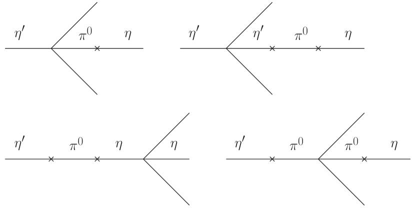
Figure 1: Feynman diagrams of the contributions with two $\Delta I=1$ insertions. The lines that are not tagged correspond to either charged or neutral pions, depending on the decay channel.

The LO ($\mathcal{O}\left(\delta^{0}\right)$) Lagrangian and relevant terms in the NLO ($\mathcal{O}\left(\delta\right)$) Lagrangian of the large $N_{c}$ ChPT contributing to IB effects in the reactions under study read [15, 20]

$$\mathcal{L}_{(0)}= \,\frac{F^{2}}{4}\left(\langle\partial_{\mu}U^{\dagger}\partial^{\mu}U\rangle+\langle U^{\dagger}\chi+\chi^{\dagger}U\rangle\right)-\frac{1}{2}M_{0}^{2}\eta_{1}^{2},$$

$$\mathcal{L}^{\rm IB}_{\text{(1)}}= \,L_{5}\langle\partial_{\mu}U^{\dagger}\partial^{\mu}U(U^{\dagger}\chi+\chi^{\dagger}U)\rangle$$

$$+L_{8}\langle U^{\dagger}\chi U^{\dagger}\chi+\chi^{\dagger}U\chi^{\dagger}U\rangle-i\frac{F\Lambda_{2}}{2\sqrt{6}}\eta_{1}\langle U^{\dagger}\chi-\chi^{\dagger}U\rangle,$$ (1)

where $U$ contains the pseudo-Nambu-Goldstone bosons, $F$ is the pion decay constant in the chiral limit, the singlet $\eta_{1}=\left(C_{0}\eta+C_{0}^{\prime}\eta^{\prime}\right)$ is a mixture of $\eta$ and $\eta^{\prime}$, $M_{0}$ is the U(1)_A anomaly contribution to the $\eta_{1}$ mass, $L_{5}$, $L_{8}$ and $\Lambda_{2}$ are low-energy constants (LECs), $\chi=2B_{0}\mathcal{M}$, $B_{0}$ is related to the quark condensate, and $\mathcal{M}$ is the light quark mass matrix, $\mathcal{M}=\text{diag}(m_{u},m_{d},m_{s})=\mathds{1}(m_{u}+m_{d}+m_{s})/3+\lambda_{3}(m_{u}-m_{d})/{2}+\lambda_{8}(\hat{m}-m_{s})/{\sqrt{3}}$, with $\lambda_{3,8}$ the Gell-Mann matrices. As shown in Ref. [26], the IB effects come from operators with $I=1$, which is the $\lambda_{3}$ term of the quark-mass matrix. This implies that all isospin-breaking insertions (vertices) considered here will change isospin by one unit.

Contributions with two IB insertions to the $\eta^{\prime}$ decays are depicted in Fig. 1. These contributions read

$$\mathcal{M}^{\rm IB}_{\pi^{0}}= \left[B_{0}(m_{u}-m_{d})\right]^{2}\left\{\left[\left(\frac{\kappa C_{\eta}C^{\prime}_{\eta}}{\Delta_{\eta^{\prime}\pi}}-\frac{C_{\eta^{\prime}}C^{\prime}_{\eta^{\prime}}}{\kappa\Delta_{\eta\pi}}\right)\frac{1}{\Delta_{\eta^{\prime}\eta}}\right.\right.$$

$$\left.-2\frac{C_{\eta}}{\Delta_{\eta\pi}}\left(\frac{C_{\pi}}{\Delta_{\eta\pi}}+\frac{C^{\prime}_{\pi}}{\kappa\Delta_{\eta^{\prime}\pi}}\right)+3\frac{C^{\prime}_{\eta^{\prime}}C_{\eta}}{C_{q}C_{q}^{\prime}\Delta_{\eta^{\prime}\pi}\Delta_{\eta\pi}}\right]$$

$$\left.\frac{}{}\mathcal{M}_{\eta^{\prime}\to\eta\pi\pi}^{\rm ChPT}+3\frac{C_{0}C_{\eta}}{F^{2}\Delta_{\eta\pi}}\right\},$$ (2)

$$\mathcal{M}^{\rm IB}_{\pi^{\pm}}= \,\left[B_{0}(m_{u}-m_{d})\right]^{2}\left[\left(\frac{\kappa C_{\eta}C^{\prime}_{\eta}}{\Delta_{\eta^{\prime}\pi}}-\frac{C_{\eta^{\prime}}C^{\prime}_{\eta^{\prime}}}{\kappa\Delta_{\eta\pi}}\right)\right.$$

$$\left.\frac{\mathcal{M}_{\eta^{\prime}\to\eta\pi\pi}^{\rm IC}}{\Delta_{\eta^{\prime}\eta}}+\frac{C^{\prime}_{\eta^{\prime}}C_{\eta}\mathcal{M}_{\pi^{0}\to\pi^{+}\pi^{-}\pi^{0}}^{\rm IC}}{\Delta_{\eta^{\prime}\pi}\Delta_{\eta\pi}}+\frac{C_{\pm}C_{\eta}}{3F^{2}\Delta_{\eta\pi}}\right],$$

where the subscript $\pi^{0}$ ($\pi^{\pm}$) in the amplitude refers to the decay channel with two neutral (charged) pions, $\mathcal{M}_{\eta^{\prime}\to\eta\pi\pi}^{\rm IC}$ and $\mathcal{M}_{\pi^{0}\to\pi^{+}\pi^{-}\pi^{0}}^{\rm IC}$ are the isospin conserving amplitudes (given in Appendix A), $\Delta_{\varphi_{1}\varphi_{2}}\equiv M_{\varphi_{1}}^{2}-M_{\varphi_{2}}^{2}$, and

$$C^{(\prime)}_{\phi} =-C_{q}^{(\prime)}-\frac{\sqrt{2}\Lambda_{2}}{3}C_{1}^{(\prime)}+\frac{4L_{5}}{F^{2}}C_{q}^{(\prime)}M^{2}_{\phi}-16\frac{L_{8}C_{q}^{(\prime)}}{F^{2}},$$

$$C_{\pm} =C_{q}^{\prime}+\frac{\sqrt{2}\Lambda_{2}}{3}C_{1}^{\prime}+12\frac{L_{5}}{F^{2}}C_{q}^{\prime}\Delta_{\eta\pi}+32\frac{L_{8}C_{q}^{\prime}}{F^{2}},$$

$$C_{0} =C_{q}^{\prime}+\frac{\sqrt{2}\Lambda_{2}}{3}C_{1}^{\prime}+32\frac{L_{8}C_{q}^{\prime}}{F^{2}},$$

$$C_{1}^{(\prime)} =\sqrt{2}C_{q}^{(\prime)}\mp C_{s}^{(\prime)}\ \quad\kappa=\frac{C_{q}}{C^{\prime}_{q}},$$ (3)

with $C_{q}^{(\prime)}$ and $C_{s}^{(\prime)}$ related to the $\eta$-$\eta^{\prime}$ mixing angles in the two mixing-angle scheme [15, 27, 28] (see Appendix A or Ref. [29] for explicit expressions).

The $Q$ parameter will be extracted from the IB unit disk distribution using the following relation [4, 8],

$$B_{0}(m_{d}-m_{u})=\frac{M_{K}^{2}}{M_{\pi}^{2}}\frac{M_{K}^{2}-M_{\pi}^{2}}{Q^{2}}+\mathcal{O}\left(m_{q}^{3}\right).$$ (4)

We account for $\pi\pi$ final state interactions with the $N/D$ unitarization method [24, 25] as of Ref. [20], and the $\eta\pi$ rescattering ($t$- and $u$-channels) in these decays is negligible [30, 31]. Details of these partial-wave amplitudes can be found in Ref. [20].

III Unit disk mapping

Consider a three-body decay with an initial particle of mass $m$ and final-state particles of masses $m_{1}$, $m_{2}$ and $m_{3}$. Let $m_{12}$ and $m_{23}$ denote the invariant masses of particles 1 and 2, and particles 2 and 3, respectively. The Dalitz plot boundary is determined by solving the equation $B\left(m_{12}^{2},m_{23}^{2}\right)=\pm 1$ with $B\left(m_{12}^{2},m_{23}^{2}\right)$ given by [32]

$$B\left(m_{12}^{2},m_{23}^{2}\right)\equiv\frac{2E_{2}^{*}E_{3}^{*}+m_{2}^{2}+m_{3}^{2}-m_{23}^{2}}{2q_{2}^{*}q_{3}^{*}},$$ (5)

where $E_{2(3)}^{*}$ and $q_{2(3)}^{*}$ represent the energy and the magnitude of the three-momentum of particle $2(3)$ in the center-of-mass (c.m.) frame of particles 1 and 2.

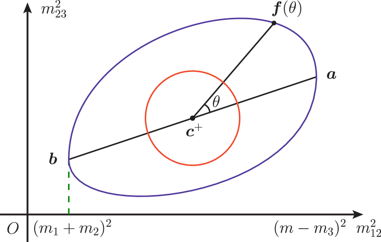
Figure 2: Illustration of the mapping from a unit disk $D$ to a Dalitz plot $B$, where $m$ is the mass of initial state particle, and $m_{i}~(i=1,2,3)$ are masses of final state particles.

A one-to-one mapping from a unit circle $D$ to the boundary of the Dalitz plot $B$, denoted as $\bm{f}:D\rightarrow B$, can be constructed as illustrated in Fig. 2. The mapping is defined by

$$\bm{f}:\theta\mapsto\left(m_{12}^{2},m_{23}^{2}\right)=\left(L(\theta),R(\theta)\right),$$ (6)

where $L(\theta)$ is the solution to the equation

$$B\big{(}m_{12}^{2},S\left(m_{12}^{2},\theta\right)\big{)}=\left\{\begin{array}[]{cl}1&\text{ for }\theta\in[0,\pi)\\ -1&\text{ for }\theta\in[\pi,2\pi)\end{array}\right.$$ (7)

with respect to $m_{12}^{2}$, and $R(\theta)=S\big{(}L(\theta),\theta\big{)}$. Here, $S(m_{12}^{2},\theta)$ represents the value of $m_{23}^{2}$ for a given $m_{12}^{2}$ and $\theta$. The center of the Dalitz plot $\bm{c}^{+}\equiv(\bm{a}+\bm{b})/2$ is mapped to the origin of the unit circle, where the two-component vectors $\bm{a}$ and $\bm{b}$ are the two endpoints of the Dalitz plot along the $m_{12}^{2}$ axis. The one-to-one mapping from the entire Dalitz plot to the unit disk, with $D$ as its boundary, can then be constructed (technical details of this mapping are provided in Appendix B).

In constructing the conventional Dalitz plot, the limits in the integral for the total width depend on the masses of the particles involved in the process. When changing the integration variables to those of the unit disk, the dependence on the masses will be transferred to the Jacobian

$$|J|=r\left(\bm{f}(\theta)-\bm{c}^{+}\right)^{2}$$ (8)

of the transformation, where $r$ is the radial coordinate of the unit disk. The three-body partial width can then be expressed as

$$\Gamma =\int dm_{12}^{2}dm_{23}^{2}\frac{d^{2}\Gamma}{dm_{12}^{2}dm_{23}^{2}}$$

$$={\int_{0}^{1}dr\int_{0}^{2\pi}d\theta\left|J\right|\frac{d^{2}\Gamma}{dm_{12}^{2}dm_{23}^{2}}}.$$ (9)

Thus, the difference in partial widths for the $\eta^{\prime}\to\eta\pi^{0}\pi^{0}$ and $\eta^{\prime}\to\eta\pi^{+}\pi^{-}$ decays is

$$2\Gamma_{\pi^{0}}-\Gamma_{\pi^{\pm}}=\int_{0}^{1}dr\int_{0}^{2\pi}d\theta\,d\Gamma^{\prime}_{\text{diff}},$$ (10)

where the difference width is defined as

$$d\Gamma_{\text{diff}}^{\prime}(r,\theta)\equiv|J_{\pi^{0}}|\frac{d^{2}\Gamma_{\pi^{0}}}{dm_{12}^{2}dm_{23}^{2}}(r,\theta)-|J_{\pi^{\pm}}|\frac{d^{2}\Gamma_{\pi^{\pm}}}{dm_{12}^{2}dm_{23}^{2}}(r,\theta).$$ (11)

However, this expression involves a large background term $(|J_{\pi^{0}}|-|J_{\pi^{\pm}}|)|\mathcal{M}_{\textrm{IC}}|^{2}$, where $\mathcal{M}_{\textrm{IC}}$ is the isospin conserving (IC) amplitude. Therefore, instead of using the previous expression, to generate the difference disk we use

$$d\Gamma_{\text{diff}}(r,\theta)\equiv\frac{d^{2}}{dm_{12}^{2}dm_{23}^{2}}\left[\Gamma_{\pi^{0}}(r,\theta)-\Gamma_{\pi^{\pm}}(r,\theta)\right].$$ (12)

Since the theoretical decay width $d^{2}\Gamma/drd\theta$ must coincide with that obtained from experimental data, each Jacobian involved in changing to $(m_{12}^{2},m_{23}^{2})$ will be included as a factor of each differential decay width obtained from experimental data.

The decay amplitude for each decay contains both the IC and IB contributions. Since the former is the same for both decays, we have

$$d\Gamma_{\text{diff}}(r,\theta)=2\operatorname{Re}\!\left({\mathcal{M}_{\rm IC}^{*}}\mathcal{M}_{\rm IB}\right)+\mathcal{O}\left(Q^{-8}\right),$$ (13)

where $\mathcal{M}_{\text{IC}}$ is the IC amplitude, and $\mathcal{M}_{\text{IB}}$ is the difference between the $\eta^{\prime}\to\eta\pi^{0}\pi^{0}$ and $\eta^{\prime}\to\eta\pi^{+}\pi^{-}$ amplitudes. Notice that all the amplitudes have been unitarized to account for the $\pi\pi$ rescattering as in Ref. [20]. The $\eta\pi$ rescattering in these decays is negligible [30, 31, 20].

The factor $\Delta_{J}\equiv 1-{\left|J_{\pi^{\pm}}\right|}/{\left|J_{\pi^{0}}\right|}$ signifies the difference between the unit disk mapping of the Dalitz plot regions for the decays. It is also an IB effect and is proportional to $M_{\pi^{\pm}}^{2}-M_{\pi^{0}}^{2}$ to a very good approximation. Numerically, $\Delta_{J}$ is in the range $\in[10.2,13.3]\%$. The term in Eq. (13) is proportional to $1/Q^{4}$, which allows it to probe the $Q$ parameter at the same level of sensitivity as the $\eta\to 3\pi$ decays.

IV Extraction of $Q$

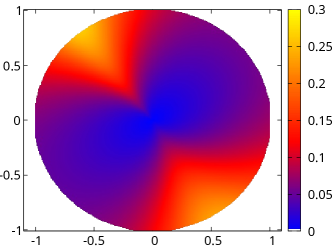
Figure 3: Unnormalized Dalitz disk of the $\eta^{\prime}\to\eta\pi^{+}\pi^{-}$ decay generated with the BESIII model [6].

We utilize the Dalitz plot distributions measured by BESIII, which are based on samples of $3.5\times 10^{6}$ and $5.6\times 10^{5}$ events for $\eta^{\prime}\to\eta\pi^{+}\pi^{-}$ and $\eta^{\prime}\to\eta\pi^{0}\pi^{0}$, respectively, obtained from $1.31\times 10^{9}$ $J/\psi$ events [6]. These samples amount to only about 1/8 of the full BESIII data set [7]. The Dalitz plot distribution is parameterized by an expansion around the center of the Dalitz plot as [6]

$$\frac{d^{2}\Gamma}{dXdY}=N(1+aY+bY^{2}+dX^{2}+...),$$ (14)

with the Dalitz plot distribution parameters $a,b$ and $d$, and expansion variables $X$ and $Y$

$$X_{\pi^{\pm}} \equiv\frac{\sqrt{3}(T_{\pi^{+}}-T_{\pi^{-}})}{M_{\eta^{\prime}}-M_{\eta}-2M_{\pi^{\pm}}},\quad X_{\pi^{0}}\equiv\frac{\sqrt{3}|T_{\pi^{0}_{1}}-T_{\pi^{0}_{2}}|}{M_{\eta^{\prime}}-M_{\eta}-2M_{\pi^{0}}},$$

$$Y \equiv\frac{M_{\eta}+2M_{\pi f}}{M_{\pi f}}\frac{T_{\eta}}{M_{\eta^{\prime}}-M_{\eta}-2M_{\pi f}}-1,$$ (15)

where $T_{i}$ is the kinetic energy of particle $i$, and $M_{\pi f}$ corresponds either to the final state charged or neutral pion mass depending on the decay channel. The normalization factor $N$ in the BESIII model [6] can be obtained from the branching fraction for each decay channel. The unit disk distribution generated using the BESIII model for the Dalitz plot distribution of $\eta^{\prime}\to\eta\pi^{+}\pi^{-}$ is shown in Fig. 3.

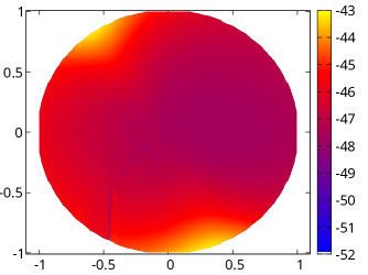
Figure 4: Dalitz disk of the difference between the charged and neutral decays generated using the BESIII data in Ref. [6].

We divide the unit disk into bins in the following way: we partition the circumscribed square of the unit circle into $10^{4}$ identical bins and then consider those that lay inside the unit disk to be the ones whose coordinates accomplish the relation $\sqrt{x^{2}+y^{2}}\leq 1$. In this way, we obtain a total of 7837 bins (0.2% away from the exact relation between the areas of the unit circle and its circumscribed square). The unit disk distribution for each decay is obtained from the constructed mapping using a Monte Carlo run with 7000 points per bin, which generates randomly the $a,b$ and $d$ parameters with a normal distribution according to their mean values, errors and correlations from the BESIII measurements [6] (listed in Appendix C). Furthermore, we also fit the overall normalization of each disk to account for the difference in theoretical and experimental partial widths. Then, subtracting the differential decay width of one disk from the other, bin by bin, we obtain a unit disk distribution of the difference, as shown in Fig. 4.

Since the $3L_{2}+L_{3}$ term compellingly dominate over the other NLO terms ($L_{5}$, $L_{8}$ and $\Lambda_{2}$) in the IC amplitudes [20], we keep $L_{2}$, $L_{3}$ and $Q$ as free parameters, along with the normalization of each disk, while setting $L_{5}=2.1\times 10^{-3}$, $L_{8}=0.8\times 10^{-3}$, and $\Lambda_{2}=0.3$ from fit 3 of Ref. [20]. The parameters are fitted to the unit disk of the difference, and we obtain

$$L_{2} =1.01(3)\times 10^{-3},\quad L_{3}=-4.40(10)\times 10^{-3},$$

$$Q =22.3(7),\quad N_{\pi^{\pm}}=108.7(4),\quad N_{\pi^{0}}=61.8(4),$$ (16)

with $\chi^{2}/\text{dof}=18549/7832$. We have checked that if we use other values for $L_{5}$, $L_{8}$ and $\Lambda_{2}$ from the other fits in the same reference instead, the result on $Q$ remains unchanged. As shown in Table 1, the $Q$ value determined in this way is compatible with previous phenomenological [17, 33, 34, 35, 36, 37, 38, 39] (see Ref. [8] for a review) and lattice [40] determinations. The uncertainty on $Q$ is also comparable to the ones obtained from $\eta\to 3\pi$ in previous studies. Therefore, once the full BESIII data set (8 times larger than the one used here) is analyzed, the uncertainty on $Q$ will be significantly reduced.

Table 1: Comparison between our determination of the $Q$ parameter and previous determinations.

$Q$	Refs.
24.3	from Dashen’s theorem [41]
$22.7\pm 0.8$	A. V. Anisovich & H. Leutwyler [17]
$23.1\pm 0.7$	K. Kampf et al. [35]
$22.1\pm 0.7$	G. Colangelo et al. [38]
$21.50\pm 0.97$	M. Albaladejo & B. Moussallam [39]
$23.3\pm 0.5$	FLAG $(N_{f}=2+1)$ [40]
$22.5\pm 0.5$	FLAG $(N_{f}=2+1+1)$ [40]
$22.3\pm 0.7$	this work

V Conclusions

In this Letter, a novel method for determining the light quark mass ratio parameter $Q$ is proposed. This method extracts symmetry breaking effects from symmetry conserved three-body decays by constructing unit disk distributions. We successfully apply the method to the decays $\eta^{\prime}\to\eta\pi^{0}\pi^{0}$ and $\eta^{\prime}\to\eta\pi^{+}\pi^{-}$. Using the BESIII data for these two decays published in Ref. [6], we obtain $Q=22.3(7)$, which is compatible with previous determinations and has a comparable uncertainty.

The method can be further refined by including the $YX^{2}$ and $X^{4}$ terms, as done in Ref. [20], which however are not available in the BESIII analysis in Ref. [6]. Additionally, the treatment of final state interactions in the decays can be improved by using a dispersion framework [22, 23].

BESIII has recently published a more thorough analysis of the $\eta^{\prime}\to\eta\pi^{0}\pi^{0}$ decays [7] with eight times more data. Although they include the $\pi\pi$ rescattering effect, they still lack the $YX^{2}$ and $X^{4}$ terms in their Dalitz plot distribution expansion. Nevertheless, once the full data set for the $\eta^{\prime}\to\eta\pi^{+}\pi^{-}$ is available, the isospin-breaking parameter $Q$ can be extracted with a significantly reduced uncertainty.

The method can also be applied to other reactions, such as decays into $J/\psi\pi\pi$ from higher charmonium(-like) states, as well as analogous decays in the bottomonium sector, to extract the IB effects therein. For such reactions with the initial state mass higher than open-charm (open-bottom) thresholds, the IB effects are expected to be more complicated since the isospin mass splittings of intermediate open-flavor mesons could play a crucial role. Using the unit disk distribution method to extract the IB effects in these reactions would be of great interest for the study of the isospin breaking dynamics in the heavy quark sector.

Appendix A Isospin conserving contribution

The ChPT Lagrangian density gives the dynamics of the pseudo-Nambu-Goldstone bosons in a nonlinear realization of the symmetry through the field $U(\phi)=\exp\left[i\frac{\sqrt{2}}{F}\phi\right]$, where

$$\phi=\left(\begin{array}[]{ccc}\frac{\pi^{0}+C_{q}\eta+C_{q}^{\prime}\eta^{\prime}}{\sqrt{2}}&\pi^{+}&K^{+}\\ \pi^{-}&\frac{-\pi^{0}+C_{q}\eta+C_{q}^{\prime}\eta^{\prime}}{\sqrt{2}}&K^{0}\\ K^{-}&{\bar{K}^{0}}&-C_{s}\eta+C_{s}^{\prime}\eta^{\prime}\end{array}\right),$$ (17)

$F$ is the pion decay constant in the chiral limit. Here we have followed the two-mixing angle scheme for the neutral mesons [15, 27, 28], where the mixing constants are parameterized in the most general form as

$$C_{q}\equiv\frac{F}{\sqrt{3}\cos\left(\theta_{8}-\theta_{0}\right)}\left(\frac{\cos\theta_{0}}{f_{8}}-\frac{\sqrt{2}\sin\theta_{8}}{f_{0}}\right),$$ (18a)

$$C_{q}^{\prime}\equiv\frac{F}{\sqrt{3}\cos\left(\theta_{8}-\theta_{0}\right)}\left(\frac{\sqrt{2}\cos\theta_{8}}{f_{0}}+\frac{\sin\theta_{0}}{f_{8}}\right),$$ (18b)

$$C_{s}\equiv\frac{F}{\sqrt{3}\cos\left(\theta_{8}-\theta_{0}\right)}\left(\frac{\sqrt{2}\cos\theta_{0}}{f_{8}}+\frac{\sin\theta_{8}}{f_{0}}\right),$$ (18c)

$$C_{s}^{\prime}\equiv\frac{F}{\sqrt{3}\cos\left(\theta_{8}-\theta_{0}\right)}\left(\frac{\cos\theta_{8}}{f_{0}}-\frac{\sqrt{2}\sin\theta_{0}}{f_{8}}\right).$$ (18d)

We will use the values of the couplings $f_{8/0}$ and the two mixing angles $\theta_{8/0}$ from Ref. [29]. The relevant operators in the NLO ($\mathcal{O}\left(\delta\right)$) Lagrangian of large $N_{c}$ ChPT are [3, 15, 20]

$$\mathcal{L}_{(1)} = L_{2}\langle\partial_{\mu}U^{\dagger}\partial_{\nu}U\partial^{\mu}U^{\dagger}\partial^{\nu}U\rangle$$ (19)

$$+(2L_{2}+L_{3})\langle\partial_{\mu}U^{\dagger}\partial^{\mu}U\partial_{\nu}U^{\dagger}\partial^{\nu}U\rangle$$

$$+L_{5}\langle\partial_{\mu}U^{\dagger}\partial^{\mu}U\left(U^{\dagger}\chi+\chi^{\dagger}U\right)\rangle$$

$$+L_{8}\langle U^{\dagger}\chi U^{\dagger}\chi+\chi^{\dagger}U\chi^{\dagger}U\rangle$$

$$-i\frac{F\Lambda_{2}}{6\sqrt{2}}\left(C_{0}\eta+C_{0}^{\prime}\eta^{\prime}\right)\langle U^{\dagger}\chi-\chi^{\dagger}U\rangle.$$

With these operators the IC amplitude for the $\eta^{\prime}\to\eta\pi\pi$ decay is

$$\mathcal{M}_{\eta^{\prime}\to\eta\pi\pi}^{\rm IC}=\frac{c_{qq}}{F^{2}}\left[\frac{M_{\pi}^{2}}{2}+\frac{24L_{8}}{F^{2}}M_{\pi}^{4}+\frac{2}{3}\Lambda_{2}M_{\pi}^{2}\right.\hskip 34.44434pt$$

$$+\frac{2(3L_{2}+L_{3})}{F^{2}}\left(s^{2}+t^{2}+u^{2}-M_{\eta^{\prime}}^{4}-M_{\eta}^{4}-2M_{\pi}^{4}\right)$$

$$\left.-\frac{2L_{5}}{F^{2}}\Delta_{\eta^{\prime}\eta\pi}M_{\pi}^{2}\right]+\frac{c_{sq}}{F^{2}}\frac{\sqrt{2}}{3}\Lambda_{2}M_{\pi}^{2},\qquad$$ (20)

where $M_{\pi}$ is the pion mass in the isospin limit, $c_{qq}=-2C_{q}C_{q}^{\prime}$, $c_{sq}=C_{q}^{\prime}Cs-C_{q}C_{s}^{\prime}$ and $F=92.2$ MeV is the physical pion decay constant. The Mandelstam variables are defined as, taking the $\eta^{\prime}\to\eta\pi^{+}\pi^{-}$ as an example, $s\equiv\left(p_{\pi^{+}}+p_{\pi^{-}}\right)^{2}$, $t\equiv\left(p_{\eta^{\prime}}-p_{\pi^{+}}\right)^{2}$, and $u\equiv\left(p_{\eta^{\prime}}-p_{\pi^{-}}\right)^{2}$; while the off-shell $\pi^{0}\to\pi^{+}\pi^{-}\pi^{0}$ amplitude reads

$$\mathcal{M}_{\pi^{0}\to\pi^{+}\pi^{-}\pi^{0}}^{\rm IC}=\frac{1}{3F^{2}}\left(3s-\Delta_{\eta^{\prime}\eta\pi}+M_{\pi}^{2}+64M_{\pi}^{4}L_{8}\frac{}{}\right.$$

$$\qquad-4\left\{6L_{2}\left[t(\Delta_{\eta^{\prime}\eta\pi}-s-t-M_{\eta^{\prime}}^{2}M_{\eta}^{2}-M_{\pi}^{4})\right]\frac{}{}\right.$$

$$\qquad-3(2L_{2}+L_{3})(s-M_{\eta^{\prime}}^{2}-M_{\eta}^{2})(s-2M_{\pi}^{2})$$

$$\qquad-M_{\pi}^{2}L_{5}(12s-5\Delta_{\eta^{\prime}\eta\pi}),$$ (21)

where $\Delta_{\eta^{\prime}\eta\pi}=M_{\eta^{\prime}}^{2}+M_{\eta}^{2}+2M_{\pi}^{2}$.

We account for $\pi\pi$ final state interactions with the $N/D$ unitarization method [24, 25] as of Ref. [20], and the $\eta\pi$ rescattering ($t$- and $u$-channels) in these decays is negligible [30, 31]. In doing so, the total amplitude is expressed in terms of partial waves. For this process the relevant partial waves are those with $J=0,2$, since the two-pion system must have $I=0$ and higher angular momentum contributions are suppressed by more powers of momenta. The unitarized amplitude reads [20]

$$\mathcal{M}(s,t,u)= \,\sum_{J}32\pi(2J+1)P_{J}(\cos\theta_{\pi})$$

$$\times\frac{\left.\mathcal{M}_{J}\right|_{\text{tree}}(s)}{1-16\pi B_{0}(s)\left.\mathcal{T}_{J}^{0}(s)\right|_{\text{tree}}},$$ (22)

where the $\mathcal{M}_{J}|_{\text{tree}}(s)$ is the partial-wave amplitude of total angular momentum $J$ at tree level, $\mathcal{T}^{0}_{J}(s)\big{|}_{\text{tree}}$ is the $I=0$ $\pi\pi$ scattering amplitude with total angular momentum $J$ at tree level, and

$$16\pi^{2}B_{0}(s)=C-\rho(s)\log\frac{\rho(s)+1}{\rho(s)-1},$$ (23)

being $\rho=\sqrt{1-4M_{\pi}^{2}/s}$ and $C$ a constant. Details of these partial-wave amplitudes can be found in Ref. [20].

Appendix B Construction of the mapping

In this appendix, we introduce the construction of the mapping from the Dalitz plot to the unit disk. We first describe the total boundary of the disk dividing it into two segments $\left(D=D^{+}\cup D^{-}\right)$:

$$D^{+}=\left.\left\{\frac{y}{\sqrt{1-x^{2}}}=~~1~\right|x\in[-1,1]\right\},$$ (24a)

$$D^{-}=\left.\left\{\frac{y}{\sqrt{1-x^{2}}}=-1~\right|x\in[-1,1]\right\},$$ (24b)

where $x$ and $y$ are, respectively, the usual abscissa and ordinate Cartesian coordinates. The segment represented by eq. (24a) is the upper part of the disk ($y\geq 0$), while that of eq. (24b) is the lower part ($y\leq 0$).

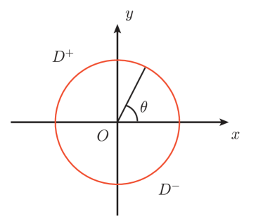
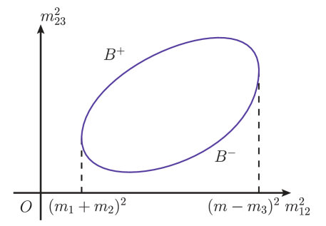
Figure 5: Left: the unit disk with its boundary divided into two segments, $D^{+}$ for $\sin\theta\geq 0$ and $D^{-}$ for $\sin\theta\leq 0$. Right: The two segments of the boundary of a conventional Dalitz plot where $B^{+}$ and $B^{-}$ correspond to $\cos\theta_{23}=1$ and $\cos\theta_{23}=-1$, respectively (see eq. (27)).

The boundary can be parameterized by the angle subtended by each point of $D$ with respect to the $x>0$ axis, so that $\theta=0$ corresponds to the maximum value of $m_{12}$:

$$x=\cos\theta,\quad y=\sin\theta,\quad\theta\in[0,2\pi).$$ (25)

Then the boundary $D$ depends only on $\theta$ (see the left plot of Fig. 5).

The boundary of the conventional Dalitz plot is set to be a function of the invariant masses square $m_{12}^{2}=(p_{1}+p_{2})^{2}$ and $m_{23}^{2}=(p_{2}+p_{3})^{2}$, constrained by kinematics. It is also divided into two segments $\left(B=B^{+}\cup B^{-}\right)$ (see the right panel of Fig. 5):

$$B^{\pm}=\left.\left\{B\left(m_{12}^{2},m_{23}^{2}\right)=\pm 1~\right|m_{12}\in[m_{1}+m_{2},m-m_{3}]\right\},$$ (26)

where $B\left(m_{12}^{2},m_{23}^{2}\right)$ is set to be the angle between the three-momenta $\vec{q}_{2}^{\,*}$ and $\vec{q}_{3}^{\,*}$ in the c.m. frame of particles 1 and 2. For 3-body decay [32]

$$B\left(m_{12}^{2},m_{23}^{2}\right)\equiv\cos\theta_{23}=\frac{2E_{2}^{*}E_{3}^{*}+m_{2}^{2}+m_{3}^{2}-m_{23}^{2}}{2q_{2}^{*}q_{3}^{*}},$$ (27)

where $E_{i}^{*}$ and $q_{i}^{*}$ are the energy and the magnitude of the three-momentum of particle $i=2,3$ in c.m. frame of particles 1 and 2. Both of $E_{i}^{*}$ and $q_{i}^{*}$ are all just functions of $m_{12}$. Furthermore, the equation of a Dalitz plot boundary, $[B\left(m_{12}^{2},m_{23}^{2}\right)]^{2}=1$, can also be expressed as the Kibble cubic function with the following explicit form:

$$stu+2(m_{1}^{2}m_{2}^{2}m_{3}^{2}+p^{2}m_{1}^{2}m_{2}^{2}+p^{2}m_{2}^{2}m_{3}^{2}+p^{2}m_{3}^{2}m_{1}^{2})=$$

$$s(m_{1}^{2}m_{2}^{2}\hskip-1.42262pt+\hskip-1.42262ptp^{2}m_{3}^{2})+t(m_{2}^{2}m_{3}^{2}\hskip-1.42262pt+\hskip-1.42262ptp^{2}m_{1}^{2})+u(m_{3}^{2}m_{1}^{2}\hskip-1.42262pt+\hskip-1.42262ptp^{2}m_{2}^{2}),$$

where $s=m_{12}^{2}$, $t=m_{23}^{2}$, $u=m_{13}^{2}=m^{2}+m_{1}^{2}+m_{2}^{2}+m_{3}^{2}-m_{12}^{2}-m_{23}^{2}$ and $m$ is the mass of the initial particle.

It is easy to obtain the coordinates in the conventional Dalitz plot where $m_{12}$ has its maximum and minimum values, which we call, respectively, $\bm{a}=(a_{1},a_{2})$ and $\bm{b}=(b_{1},b_{2})$, through Eq. (27); this is, $b_{1}=\left(m_{12}^{2}\right)_{\rm min}$, $a_{1}=\left(m_{12}^{2}\right)_{\rm max}$, these conditions fix the second components of both vectors. We also define $\bm{c}^{\pm}=(\bm{a}\pm\bm{b})/2$, which is used to set the center of the disk and the orientation of the Cartesian coordinate-system with respect to the Dalitz plot coordinate system (see bellow). In this way, $\bm{c}^{-}$ is a vector pointing from the center of the Dalitz plot to the point with the maximum value of $m_{12}^{2}$, and the mean $\bm{c}^{+}$ is a vector pointing from the origin to the center.

Consider a mapping $S:[(m_{1}+m_{2})^{2},(m-m_{3})^{2}]\times[0,2\pi)\to[(m_{2}+m_{3})^{2},(m-m_{1})^{2}]$ with the following explicit form:

$${\small S\big{(}m_{12}^{2},\theta\big{)}=\left\{\begin{array}[]{ll}\!\!\tan{\beta}\left(m_{12}^{2}-c_{1}^{+}\right)+c_{2}^{+}&\text{for }\beta\neq\frac{\pi}{2},\frac{3\pi}{2},\\ \!\!\text{Solution of }B\left(c^{+}_{1},m_{23}^{2}\right)=~~1&\text{for }\beta=\frac{\pi}{2},\\ \!\!\text{Solution of }B\left(c^{+}_{1},m_{23}^{2}\right)=-1&\text{for }\beta=\frac{3\pi}{2},\end{array}\right.}$$ (28)

where $\beta=\theta+\alpha$, $\theta\in[0,2\pi)$, and $\alpha$ is the angle between the $m_{12}$ axis and $\bm{c}^{-}$. One has

$$\tan\alpha=\frac{c^{-}_{2}}{c^{-}_{1}}=\frac{m_{1}m_{3}-mm_{2}}{(m-m_{3})(m_{1}+m_{2})}.$$ (29)

For the decays at hand, we choose the final state pion pair to be particles 1 and 2 and $\eta$ as particle 3. Thus, for both decays, we find $\tan\alpha=-1/2$, and $\alpha=-\arctan(1/2)$.

Then one can construct a one-to-one mapping from the unit circle $D$ to the Dalitz plot boundary $B$, $\bm{f}:D\to B$ or equivalently,

$$\bm{f}:\theta\mapsto\left(m_{12}^{2},m_{23}^{2}\right)\equiv\left(L(\theta),R(\theta)\right).$$ (30)

Here, $L(\theta)$ is the solution to the equation

$$B\big{(}m_{12}^{2},S\left(m_{12}^{2},\theta\right)\big{)}=\left\{\begin{array}[]{cl}1&\text{ for }\theta\in[0,\pi),\\ -1&\text{ for }\theta\in[\pi,2\pi)\end{array}\right.$$ (31)

with respect to $m_{12}^{2}$, and $R(\theta)=S\big{(}L(\theta),\theta\big{)}$. Thus, $\bm{c}^{+}$ gives the coordinates of the center of the disk in the invariant-mass coordinate system of the Dalitz plot and $\bm{c}^{-}$ the angle $\alpha$ between the $x$ and $m_{12}^{2}$ axes.

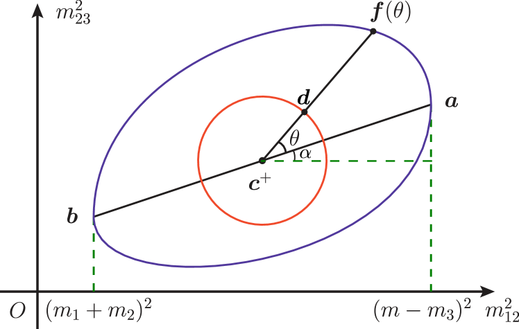
Figure 6: Mapping from a Dalitz plot to the unit disk, where $m$ is the mass of initial state particle, and $m_{i}~(i=1,2,3)$ are masses of final state particles.

Up to now, we have constructed a mapping from $D$ to $B$ with $\bm{f}(\theta)=\big{(}L(\theta),R(\theta)\big{)}$. Next we can use the boundary mapping $\bm{f}$ to construct a mapping $\bm{F}$ from the conventional Dalitz plot to the unit disk. $\bm{F}:\left(m_{12}^{2},m_{23}^{2}\right)\mapsto(r,\theta)$. The procedure is as follows. If $\left|\bm{d}-\bm{c}^{+}\right|=0$, where $\bm{d}=\left(m_{12}^{2},m_{23}^{2}\right)$ is any element belonging to the Dalitz plot (see to Fig. 6), then $r=0$; otherwise,

$$\cos\theta=\frac{\left(\bm{d}-\bm{c}^{+}\right)\cdot\bm{c}^{-}}{\left|\bm{d}-\bm{c}^{+}\right|\hskip 2.15277pt\left|\bm{c}^{-}\right|},\quad r=\frac{\left|\bm{d}-\bm{c}^{+}\right|}{\left|\bm{f}(\theta)-\bm{c}^{+}\right|}.$$ (32)

For the division of the unit disk into bins, we use the Cartesian coordinates: we first generate a mesh in the circumscribed square of the unit circle with lines parallel to the $x$ and $y$ axes in eq. (25). To do this, we generate 100 equidistant lines parallel to the former and 100 parallel to the latter. This divides the square into 10,000 same-size bins. Afterwards we select those that fulfill $r\leq 1$; after neglecting those bins outside the unit circle we are left with 7,837 bins. The percentage of accepted bins is close to the ratio of the areas of the unit disk and the unit square, which is $\pi/4\approx 78.54\%$.

Appendix C Input Dalitz plot distribution parameters

The Dalitz plot distribution parameters for the $\eta^{\prime}\to\eta\pi^{0}\pi^{0}$ and $\eta^{\prime}\to\eta\pi^{+}\pi^{-}$ decays extracted by the BESIII Collaboration are [6]

$$a_{\pi^{0}}=-0.087\pm 0.009,\hskip 4.30554ptb_{\pi^{0}}=-0.073\pm 0.006,$$

$$\hskip 55.97205ptd_{\pi^{0}}=-0.074\pm 0.004,$$ (33a)

$$a_{\pi^{\pm}}=-0.056\pm 0.004,\hskip 2.15277ptb_{\pi^{\pm}}=-0.049\pm 0.006,$$

$$\hskip 55.97205ptd_{\pi^{\pm}}=-0.063\pm 0.004,$$ (33b)

where their correlation matrices were reported to be

$$C_{\pi^{0}}=\left(\begin{array}[]{c|cc}&b_{\pi^{0}}&d_{\pi^{0}}\\ \hline\cr a_{\pi^{0}}&-0.495&-0.273\\ &&0.273\end{array}\right),$$ (34)

for the decay into neutral pions and

$$C_{\pi^{\pm}}=\left(\begin{array}[]{c|cc}&b_{\pi^{\pm}}&d_{\pi^{\pm}}\\ \hline\cr a_{\pi^{\pm}}&-0.417&-0.239\\ &&0.292\end{array}\right),$$ (35)

for the decay into charged pions.