Slowing Learning by Erasing Simple Features
Abstract
Prior work suggests that neural networks tend to learn low-order moments of the data distribution first, before moving on to higher-order correlations. In this work, we derive a novel closed-form concept erasure method, QLEACE, which surgically removes all quadratically available information about a concept from a representation. Through comparisons with linear erasure (LEACE) and two approximate forms of quadratic erasure, we explore whether networks can still learn when low-order statistics are removed from image classification datasets. We find that while LEACE consistently slows learning, quadratic erasure can exhibit both positive and negative effects on learning speed depending on the choice of dataset, model architecture, and erasure method.
Use of QLEACE consistently slows learning in feedforward architectures, but more sophisticated architectures learn to use injected higher order Shannon information about class labels. Its approximate variants avoid injecting information, but surprisingly act as data augmentation techniques on some datasets, enhancing learning speed compared to LEACE.
1 Introduction
The success of deep learning is due in large part to the good inductive biases baked into popular neural network architectures (Chiang et al., 2022; Teney et al., 2024). One of these biases is the distributional simplicity bias (DSB), which states that neural networks learn to exploit the lower-order statistics of the input data first– e.g. mean and (co)variance– before learning to use its higher-order statistics, such as (co)skewness or (co)kurtosis.
Recent work from Belrose et al. (2024) provides evidence for the DSB by evaluating intermediate checkpoints of a network on maximum entropy synthetic datasets which match the low-order statistics training set. They find that networks learn to perform well on the max-ent synthetic datasets early in training, then lose this ability later.
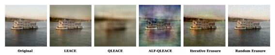
In this work, we invert the experimental setup of Belrose et al. (2024) by training networks on datasets whose low-order statistics have been made uninformative of the class label. To remove first-order information– that is, making all classes have the same mean– we use the LEAst-squares Concept Erasure (LEACE) method from Belrose et al. (2023), which provably distorts the data only as little as is necessary. For second-order information– differences in covariance between classes– we derive two novel concept erasure techniques which may be of independent interest: QLEACE, and an approximate variant ALF-QLEACE.
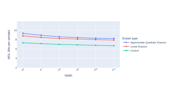
We measure the “difficulty” of learning on erased data using the prequential minimum description length (MDL) framework proposed by Voita & Titov (2020). Prequential MDL is equivalent to the area under the learning curve, where the x-axis indicates the size of the training dataset, and the y-axis is the cross-entropy loss computed on a validation set after training. Additionally, we report final losses achieved on training runs which use the entire dataset.
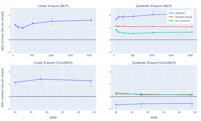
We find that LEACE is consistently effective in making learning more difficult, causing significant increases in MDL which are consistent across network architectures. Interestingly, making the network more expressive by increasing its width beyond roughly 500 or 1K neurons does not seem to reduce the MDL, either on the control set or on the LEACE’d dataset. Since we use the maximal update parametrization (Yang et al., 2021) to ensure hyperparameter transfer across network widths, this suggests LEACE makes learning more difficult even for infinite width feature-learning networks (Yang & Hu, 2020; Vyas et al., 2024).
By contrast, our quadratic erasure results are much more mixed. We found that there are multiple different ways of eliminating or reducing the amount of quadratic information present in a dataset, and each of these methods seem to yield different results. While QLEACE guarantees that all classes will have equal means and covariance matrices, it can potentially inject additional information about the class label into higher-order statistics. In some cases, this leads to a phenomenon we call backfiring where a model learns to exploit these higher-order statistics after many epochs of training, ultimately achieving lower loss than it does on the original data.
ALF-QLEACE is meant to address this problem: since it applies the same affine transformation to every datapoint independent of its class label, it cannot cause backfiring, although it leaves a fraction of the quadratically-available information intact. We also experiment with a gradient-based approach which directly optimizes the dataset to remove quadratic information, while penalizing the distance traveled from the original data. Surprisingly, these methods seem to serve as a form of data augmentation for convolutional networks, leading to a lower MDL than LEACE does. We conclude that known quadratic concept erasure methods are unreliable and should be used with caution.
2 Erasing Moments via Optimal Transport
Consider a -class classification task over jointly defined random vectors (the input data) and (the one-hot labels), taking values in and 111We frequently use the integer to refer to the element of which is at the index and elsewhere. respectively, with and each , and a predictor , chosen from a function class (presumed to contain all constant functions) so as to minimize the expectation of some in a class of loss functions.
Definition 2.1 (Polynomial Predictor).
A degree polynomial predictor is a function , where the th component of is a polynomial of degree in the components of , and is interpreted as the likelihood that is a member of class . In Einstein summation notation we have
| (1) |
where is a bias term, and each is an order coefficient tensor whose first axes are of size , and whose final axis is of size . For binary classification where , Eq. 1 reduces to the familiar quadratic form for , and a linear classifier for .
Once we allow the erasure function to depend on the class label, we can immediately draw a connection with the Monge formulation of the optimal transport problem between probability distributions. First consider the information-theoretic erasure task: given class-conditional distributions and a cost function , we seek a barycenter distribution and a set of transport maps minimizing expected cost while transporting each class to .
| (2) |
where the minimum is taken over measurable functions that map to . It’s easy to see that an exact solution to this task would eliminate all Shannon information between and , preventing unrestricted nonlinear adversaries from predicting from better than chance.222Strictly speaking, the Monge formulation of OT does not always have a solution: for example, it is impossible for any deterministic map to transport the Dirac delta distribution to a Gaussian. The Kantorovich formulation, which allows for stochastic transport maps, always has a solution, but in this work we assume the Monge problem is feasible on real-world datasets.
2.1 Extension to Polynomial Classifiers
Below, we extend Belrose et al. (2023, Theorem 3.1) to general polynomial predictors.
Theorem 2.2.
Suppose is convex in . Then if for each class and each order , the tensor of class-conditional moments is equal to the unconditional moment tensor , the trivially attainable loss cannot be improved upon.
Proof.
See Appendix A.1. ∎
We also extend Belrose et al. (2023, Theorem 3.2) to the polynomial case:
Theorem 2.3.
Suppose has bounded partial derivatives, which when off-category never vanish and do not depend on the category, i.e. for all categories . If is minimized among degree polynomial predictors by the constant predictor with , then for each order , the tensor of class-conditional moments is equal to the unconditional moment tensor .
Proof.
See Appendix A.2. ∎
As noted in Belrose et al. (2023, Theorem 3.3), this theorem applies to the popular categorical cross entropy loss .
2.2 Quadratic LEACE
The theorems of Sec. 2.1 imply that our erasure function must ensure the class-conditional mean and covariance equal the unconditional mean and covariance, but they do not specify what these unconditional moments should be. We are therefore free to select the target mean and covariance matrix so as to minimize the expected edit magnitude . Using results from optimal transport theory, we derive the optimal unconditional mean and covariance matrix, as well as the optimal class-dependent quadratic concept erasure function.
Lemma 2.4 (Gaussian Wasserstein Barycenter).
Let be Gaussian distributions with means and non-singular covariance matrices , along with non-negative weights . Let be the set of probability measures over with finite second moment. Then
| (3) |
where and is the unique positive definite satisfying the equation
| (4) |
Proof.
See Rüschendorf & Uckelmann (2002, pg. 246). ∎
Lemma 2.5 (2-Wasserstein Lower Bound).
Let be the set of probability measures over with finite second moment. Let have means and covariance matrices , with full rank. Then
| (5) |
with equality if and only if the map transports to , where
| (6) |
Proof.
See Cuesta-Albertos et al. (1996). ∎
Theorem 2.6 (Quadratic LEACE).
Let be distributions on with means , full rank covariance matrices , and weights . Let be the set of distributions on with mean and covariance matrix . Then the objective
| (7) |
is minimized by the mean and covariance matrix of the barycenter of , as defined in Lemma 2.4.
Further, for each , the optimal transport map from to the optimal is the optimal transport map from to , as defined in Lemma 2.5.
Proof.
We first consider the inner optimization problem for any fixed chosen for the outer optimization problem.
Our only constraint for each is that . Thus is feasible, with . Further, by Lemma 2.5, this choice achieves the minimum possible cost in the feasible set , equal to .
We draw the following two conclusions.
First, for the optimal choice of , defined as , the optimal transport map for each is
| (8) |
Second, we can rewrite our objective as
| (9) |
This is identical to the Gaussian barycenter objective from Lemma 2.4, except that we have restricted the feasible set to Gaussian distributions. Since the barycenter of Gaussian distributions is always Gaussian, this restriction makes no difference to the solution. Therefore the barycenter of will have mean and covariance that minimize Eq. 9, thus completing the proof. ∎
To solve for the unconditional covariance matrix, we use the fixed-point algorithm derived in Álvarez-Esteban et al. (2016). Then the optimal transport map can be computed in closed form as described above.
2.3 Approximate Label-Free Quadratic LEACE
While naïve quadratic LEACE removes quadratically available information, it also potentially injects Shannon information about the class label. Consider a dataset where each sample is a -dimensional data point from one of classes. The data naturally lies within a bounded hypercube or defined by the valid range of each dimension. By applying an erasure function specific to the class label of each sample, QLEACE effectively transforms the hypercube into characteristic hyperparallelipipeds. Neural networks of sufficient expressivity may use this information to classify data.
Approximate Label-Free QLEACE removes some quadratically available information without injecting label information by applying the same transformation to each data point. The transformation is composed of a LEACE transformation to remove linearly available information, and an ALF-QLEACE transformation to remove some quadratically available information information.
Let denote the class-conditional covariance matrix for class , and let be the average of all class-conditional covariance matrices. Perfect quadratic guardedness would imply that
| (10) |
This is trivially satisfied if is the zero matrix, but this would remove all information contained in the representation. We need a higher-rank transformation.
The rank ALF-QLEACE transformation is a projection matrix that satisfies
| (11) |
The min-max theorem implies that the rank orthogonal projection of a matrix with respect to both Frobenius and spectral norms is given by truncating its singular value decomposition to the largest singular values.
Therefore, the rank 1 projection matrix that best approximates the difference matrix for a class is given by the largest singular value of its singular value decomposition, and the optimal rank projection matrix which minimizes that projects onto the orthogonal complement of the direction that contributes most to this maximum singular value - specifically, either singular vector corresponding to the largest singular value of for the class that maximizes the norm.
The rank projection preserves as much of the original data structure as possible while still effectively removing the strongest quadratic correlations. The projection does not increase variance in any direction and is therefore guaranteed to not increase the norm for another class.
The efficacy of the projection may be improved by iteratively adding up to rank 1 erasures, each calculated on the updated class and global covariances matrices and .
2.4 Gradient-based Moment Erasure
We also experiment with a much more “direct” approach to erasing low-order class information from a dataset, using gradient-based optimization. Specifically, we initialize our synthetic dataset using the original data, and use L-BFGS (Liu & Nocedal, 1989) to optimize a loss function containing three terms: the average squared distance between each class-conditional mean and the unconditional mean, the average squared distance between each class-conditional covariance matrix and the unconditional covariance matrix, and the squared distance between the original images and their modified counterparts. We tune the weights of the three loss terms to ensure that the synthetic dataset has almost no quadratically-available information about the class label, while keeping fairly close to the original images. We also re-parameterize the images using the sigmoid function to ensure pixel values stay within the admissible range .
This approach has the benefit of not causing backfiring, and being mathematically straightforward. Unlike the other methods, however, it does not produce an “eraser” transformation that can be re-used on new datapoints.
3 Experiments
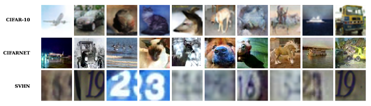
We investigate the effects of erasing simple features from three popular image classification datasets: CIFAR-10 (Krizhevsky et al., 2009), CIFARNet (Belrose et al., 2024), and Street View House Numbers (SVHN) (Netzer et al., 2011). For data augmentation we apply random crops and horizontal flips, both linear transformations which cannot recover erased information. For each dataset we examine the effects on learning of LEACE, quadratic erasure, and two approximate variants of quadratic erasure.
We use the maximal update parametrization (P) to transfer the optimal hyperparameters from narrower neural networks to wider ones (Yang et al., 2021). When scaling our MLPs to different depths, we adapt the experimental learning rate scaling exponent of proposed in Jelassi et al. (2023), and use a more conservative scaling exponent of for all other architectures,
where is the number of layers.
We also use the schedule-free AdamW optimizer proposed by Defazio et al. (2024), which allows us to train our networks for as long as is necessary to achieve convergence without fixing a learning rate decay schedule in advance.
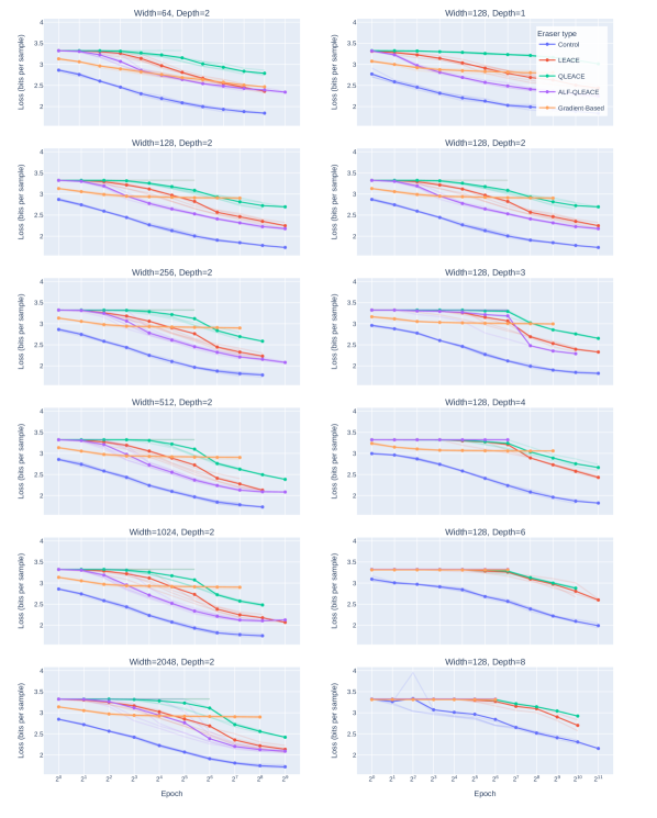
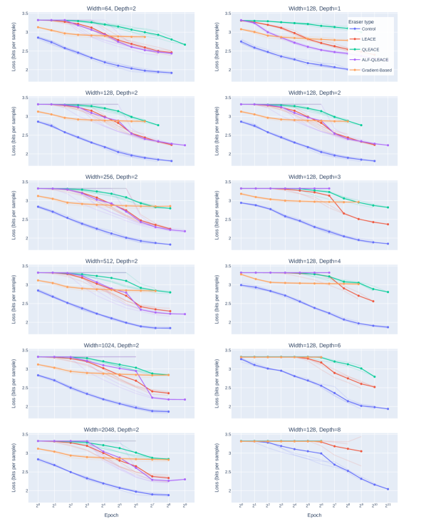
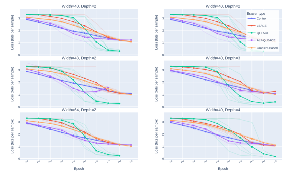
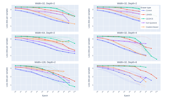
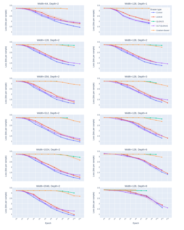
To investigate how dataset choice mediates the effects of feature erasure we train MLPs and parameter-matched LeNets on the CIFAR-10, CIFARNet, and SVHN datasets. For each combination of dataset, eraser, and architecture we track training dynamics via cross-entropy loss curves for various widths and depths and compute the prequential MDL, averaging results across five random seeds.
To investigate the effects of erasure on state-of-the-art image classification architectures, we train Swin Transformer V2 (Liu et al., 2022) and ConvNeXt V2 (Woo et al., 2023) models on the CIFAR-10 dataset. We scale the models width- and depth-wise and collect average prequential MDLs (scaling details are available in Appendix B).
Finally, we examine the effect of dataset z-score normalization on erasures.
4 Results
Linear Erasure (LEACE)
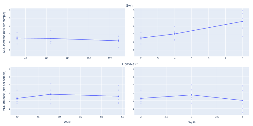
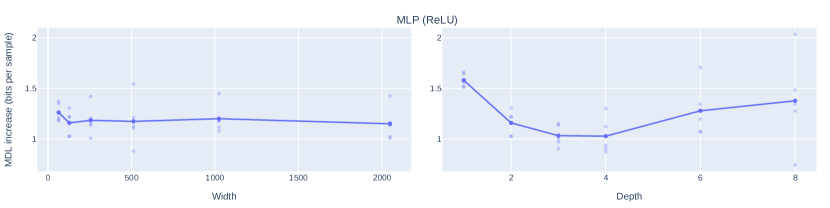
Applying LEACE to datasets consistently increases MDL and final loss across all models and tasks. This effect is roughly equal between architectures, and varies little across model widths and depths.
QLEACE
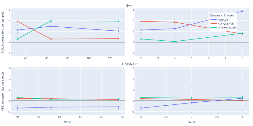
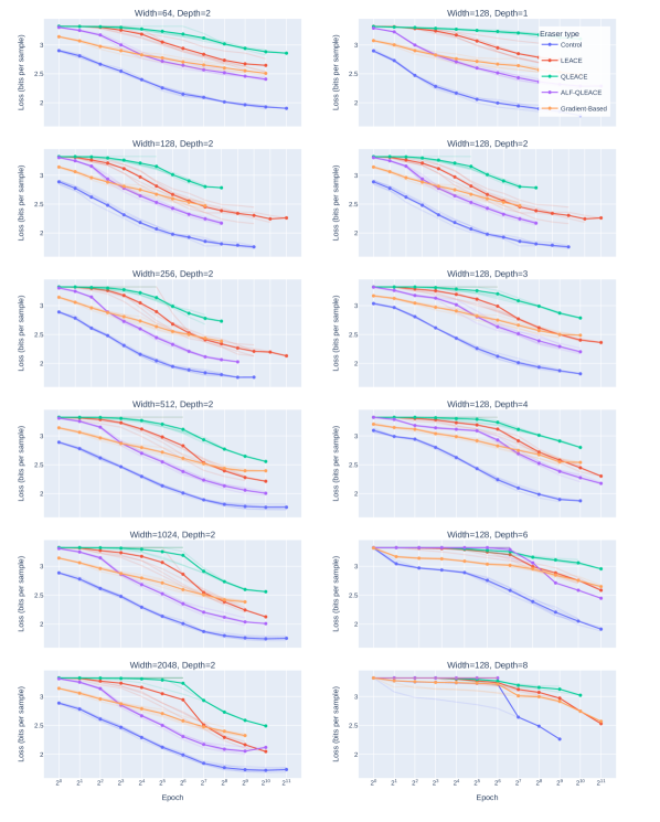
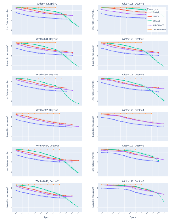
QLEACE generally produces larger MDL and loss increases than linear erasure in the feedforward networks. In state-of-the-art Swin and ConvNeXt architectures, however, the impact is mixed. QLEACE slows learning more than any other erasure methods in early epochs, with early loss surpassing models trained on linearly erased datasets (Figures 12 and 13). However, after approximately 16 epochs a sharp transition occurs: loss plummets rapidly, allowing these models to ultimately achieve lower final loss than models trained on unedited data.
We call this phenomenon “backfiring.” For Swin architectures, the prolonged high-loss phase during early training ultimately produces higher prequential MDL than unedited baselines – closely matching the MDL of LEACE-edited data. ConvNeXt models, by contrast, achieve lower overall MDL with QLEACE than with any other erasure method, even though the backfiring occurs late in training.
Additionally, backfiring occurs in all two- and three-layer MLPs on the CIFARNet dataset, suggesting that even simple networks are able to access the injected higher order information in some datasets.
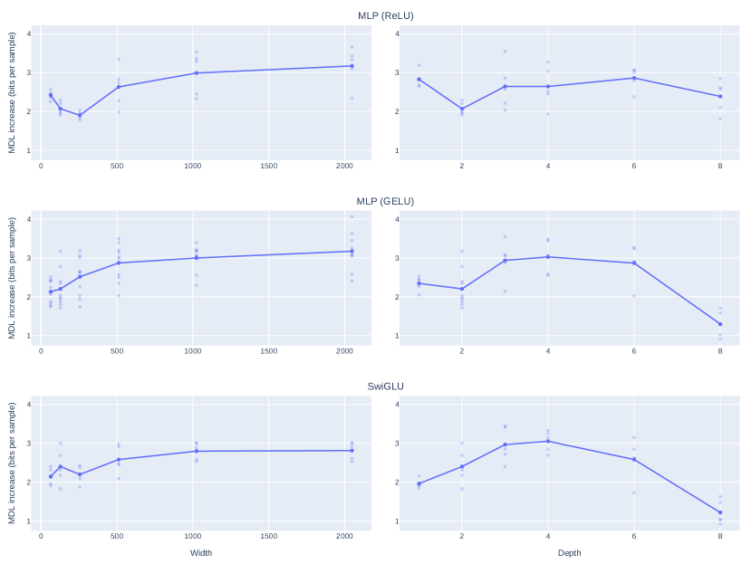
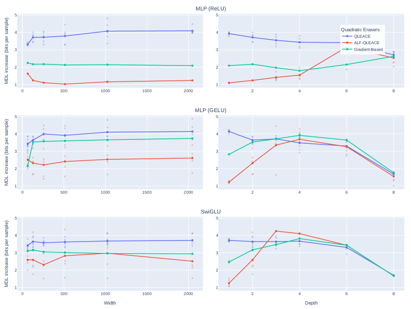
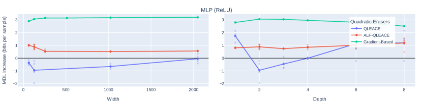
While QLEACE produces similar increases in MDL across feedforward architectures, ReLU-based MLPs tend to be more affected at greater depths, and GeLU-based MLPs and SwiGLUs in shallow settings (Figure 5).
Gradient-Based Quadratic Erasure
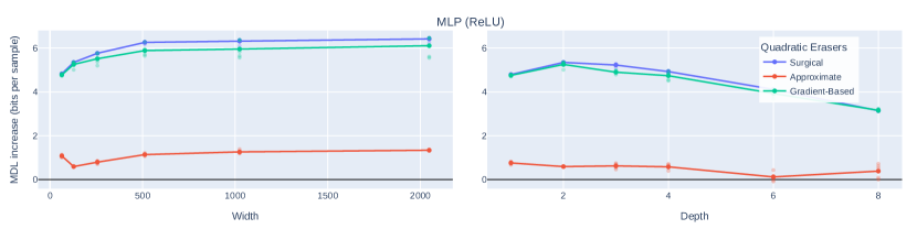
The gradient-based approach to quadratic erasure increases MDL across all architectures without producing backfiring. However, its efficacy relative to QLEACE varies, notably yielding substantially reduced MDL in feedforward networks - contexts where quadratic erasure does not produce backfiring. This disparity suggests that partial quadratic information may remain accessible even after aggressive gradient-based editing. These findings highlight potential limitations in gradient-based methods.
Approximate Quadratic Erasure (ALF-QLEACE)
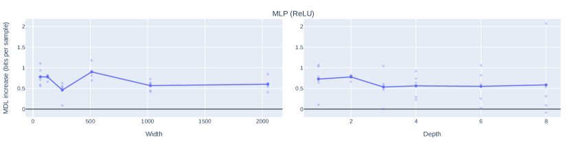
Datasets modified by ALF-QLEACE show a small increase in prequential MDL across all architectures. Surprisingly, the effect relative to LEACE is smaller in most cases, despite ALF-QLEACE applying LEACE as an initial step. This indicates that, by ablating directions along which the classes have very different variances, ALF-QLEACE is actually making the data easier to learn.
We speculated that the smaller effect of ALF-QLEACE on MDL is caused by a data augmentation effect, where its partial normalization of the data covariance matrix by removing the directions of highest variance improves learning. We examined whether z-score normalizing the CIFAR-10 dataset before erasure affected the relative increase in MDL, with ambiguous results (Table 16).
5 Conclusion
Due to the backfiring phenomena we observed in all of our quadratic concept erasure methods, we urge practitioners to exercise caution when applying them in practice. By contrast, our results suggest that LEACE is a reliable method for making features less salient and more difficult to learn.
Contributions and acknowledgements
Nora derived QLEACE and ALF-QLEACE, and wrote the mathematical parts of the paper. Lucia ran all of the experiments and analyzed the results.
We are grateful to Coreweave for providing computing resources for this project. Nora and Lucia are funded by a grant from Open Philanthropy.
Impact Statement
As discussed in Belrose et al. (2023), concept erasure methods can be used to enhance the fairness of deep learning models by making sensitive information, like gender or race, less salient. On the other hand, methods closely related to concept erasure can also be used to bypass safety training in large language models (Marshall et al., 2024). Overall, we judge that the ability to control what types of information are used by deep neural networks is beneficial for their interpretability and steerability.
References
- Álvarez-Esteban et al. (2016) Álvarez-Esteban, P. C., Del Barrio, E., Cuesta-Albertos, J., and Matrán, C. A fixed-point approach to barycenters in wasserstein space. Journal of Mathematical Analysis and Applications, 441(2):744–762, 2016.
- Belrose et al. (2023) Belrose, N., Schneider-Joseph, D., Ravfogel, S., Cotterell, R., Raff, E., and Biderman, S. Leace: Perfect linear concept erasure in closed form. arXiv preprint arXiv:2306.03819, 2023.
- Belrose et al. (2024) Belrose, N., Pope, Q., Quirke, L., Mallen, A. T., and Fern, X. Neural networks learn statistics of increasing complexity. In Forty-first International Conference on Machine Learning, 2024. URL https://openreview.net/forum?id=IGdpKP0N6w.
- Chiang et al. (2022) Chiang, P.-y., Ni, R., Miller, D. Y., Bansal, A., Geiping, J., Goldblum, M., and Goldstein, T. Loss landscapes are all you need: Neural network generalization can be explained without the implicit bias of gradient descent. In The Eleventh International Conference on Learning Representations, 2022.
- Cuesta-Albertos et al. (1996) Cuesta-Albertos, J. A., Matrán-Bea, C., and Tuero-Diaz, A. On lower bounds for the l 2-wasserstein metric in a hilbert space. Journal of Theoretical Probability, 9(2):263–283, 1996.
- Defazio et al. (2024) Defazio, A., Yang, X. A., Mehta, H., Mishchenko, K., Khaled, A., and Cutkosky, A. The road less scheduled. arXiv preprint arXiv:2405.15682, 2024.
- Jelassi et al. (2023) Jelassi, S., Hanin, B., Ji, Z., Reddi, S. J., Bhojanapalli, S., and Kumar, S. Depth dependence of p learning rates in relu mlps, 2023. URL https://arxiv.org/abs/2305.07810.
- Krizhevsky et al. (2009) Krizhevsky, A., Hinton, G., et al. Learning multiple layers of features from tiny images. 2009.
- Liu & Nocedal (1989) Liu, D. C. and Nocedal, J. On the limited memory bfgs method for large scale optimization. Mathematical programming, 45(1):503–528, 1989.
- Liu et al. (2022) Liu, Z., Hu, H., Lin, Y., Yao, Z., Xie, Z., Wei, Y., Ning, J., Cao, Y., Zhang, Z., Dong, L., et al. Swin transformer v2: Scaling up capacity and resolution. In Proceedings of the IEEE/CVF conference on computer vision and pattern recognition, pp. 12009–12019, 2022.
- Marshall et al. (2024) Marshall, T., Scherlis, A., and Belrose, N. Refusal in llms is an affine function. arXiv preprint arXiv:2411.09003, 2024.
- Netzer et al. (2011) Netzer, Y., Wang, T., Coates, A., Bissacco, A., Wu, B., and Ng, A. Y. Reading digits in natural images with unsupervised feature learning. In NIPS Workshop on Deep Learning and Unsupervised Feature Learning 2011, 2011. URL http://ufldl.stanford.edu/housenumbers/nips2011_housenumbers.pdf.
- Rüschendorf & Uckelmann (2002) Rüschendorf, L. and Uckelmann, L. On the n-coupling problem. Journal of multivariate analysis, 81(2):242–258, 2002.
- Teney et al. (2024) Teney, D., Nicolicioiu, A. M., Hartmann, V., and Abbasnejad, E. Neural redshift: Random networks are not random functions. In Proceedings of the IEEE/CVF Conference on Computer Vision and Pattern Recognition, pp. 4786–4796, 2024.
- Voita & Titov (2020) Voita, E. and Titov, I. Information-theoretic probing with minimum description length. arXiv preprint arXiv:2003.12298, 2020.
- Vyas et al. (2024) Vyas, N., Atanasov, A., Bordelon, B., Morwani, D., Sainathan, S., and Pehlevan, C. Feature-learning networks are consistent across widths at realistic scales. Advances in Neural Information Processing Systems, 36, 2024.
- Woo et al. (2023) Woo, S., Debnath, S., Hu, R., Chen, X., Liu, Z., Kweon, I. S., and Xie, S. Convnext v2: Co-designing and scaling convnets with masked autoencoders. In Proceedings of the IEEE/CVF Conference on Computer Vision and Pattern Recognition, pp. 16133–16142, 2023.
- Yang & Hu (2020) Yang, G. and Hu, E. J. Feature learning in infinite-width neural networks. arXiv preprint arXiv:2011.14522, 2020.
- Yang et al. (2021) Yang, G., Hu, E., Babuschkin, I., Sidor, S., Liu, X., Farhi, D., Ryder, N., Pachocki, J., Chen, W., and Gao, J. Tuning large neural networks via zero-shot hyperparameter transfer. Advances in Neural Information Processing Systems, 34:17084–17097, 2021.
Appendix A Concept erasure proofs
A.1 Sufficiency
See 2.2
Proof.
Let be an arbitrary polynomial predictor of degree . We can derive a lower bound on the expected loss of evaluated on as follows.
| (Jensen’s inequality) | ||||
| (Def. 2.1 and linearity) | ||||
| (by assumption) | ||||
| (definition of ) |
The trivially attainable loss is the lowest loss achievable by a constant function. Since is a constant function and was arbitrary, no can improve upon the trivially attainable loss. ∎
A.2 Necessity
See 2.3
Proof.
Fix some class . The first-order optimality condition on and yields333We are using NumPy-style indexing here, so that refers to the slice of where the final axis index is set to . This yields a “square” order- tensor whose axes are all of size .
| (12) |
Since is constant over all values of , and , the first equation in (12) reduces to:
| (13) |
where is an abuse of notation denoting the off-category partial derivative, emphasizing its independence of the category . For each , the constancy of and the fact that reduces the second part of (12) to:
| (14) |
Solving for in (13) and substituting in (14) gives us:
| (15) |
If , then all class-conditional moments are trivially equal to the unconditional moments. Otherwise, we can divide both sides by and by (using the non-vanishingness of the off-category partial derivative), yielding for each order :
thereby completing the proof. ∎
Appendix B Model scaling details
ConvNeXt and Swin models are produced using width and depth parameters, which represent base network parameters and are scaled in later stages according to a conventional structure.
In the ConvNeXt models, the base depth is scaled in the third stage to produce the depths , and width doubles in each successive stage, following standard practice for progressive feature map expansion. The Swin models follow the same general scaling structure, with the number of heads also scaling in the third stage according to .
Our ConvNeXt and Swin implementations use a reduced patch size of 1 and 2 respectively to accommodate the datasets’ small image sizes.
Appendix C Detailed results
| Architecture | Control | LEACE | ALF-QLEACE | Gradient Quadratic | QLEACE |
|---|---|---|---|---|---|
| MLP | 7.14 ± 0.05 | 8.49 ± 0.10 | 8.94 ± 0.14 | 10.02 ± 0.08 | 11.41 ± 0.00 |
| LeNet | 5.62 ± 0.02 | 6.59 ± 0.28 | 6.83 ± 0.11 | 8.71 ± 0.09 | 8.68 ± 0.24 |
| ConvNeXtV2 | 5.09 ± 0.09 | 5.20 ± 0.15 | 4.92 ± 0.05 | 5.37 ± 0.02 | 1.67 ± 0.20 |
| Swin V2 | 8.18 ± 0.03 | 9.00 ± 0.13 | 8.67 ± 1.20 | 9.29 ± 0.06 | 9.08 ± 0.13 |