Cherenkov emission by a fast-moving uncharged Schwarzschild black hole

Abstract

We demonstrate that in the presence of an external magnetic field, an uncharged classical Schwarzschild  black hole  moving superluminally in a dielectric with permittivity $\epsilon>1$ produces Cherenkov emission. This is a new physical effect: classical (non-quantum) emission of electromagnetic waves by a completely charge-neutral “particle”. The governing equations (involving General Relativity, electromagnetism, and the physics of continuous media) have no external electromagnetic source - it is the distortion of the initial electromagnetic fields by the gravity of the black hole that plays the role of a superluminally moving source. The effect relies on nonzero values of both the magnetic field and the gravitational radius, as well as on the usual Cherenkov condition on the velocity, $v/c>1/\sqrt{\epsilon}$. Unlike Cherenkov emission by a point charge, the effective source in this case is spatially distributed, with emission generated along the single Cherenkov emission cone. The emitted spectrum is red-dominated, with power $\propto dk_{z}/|k_{z}|$ for wave numbers $|k_{z}|\leq 1/R_{G}$, where $R_{G}$ is the Schwarzschild radius. We comment on possible observability of this process during black hole-neutron star mergers.

I Introduction

There is a number of classical (non-quantum) effects at the intersection of general relativity (GR), electromagnetism (EM) and physics of continuous media. Arguably, the most famous one is the Blandford-Znajek (BZ) effect (Blandford and Znajek, 1977), whereby a Kerr black hole (BH) immersed in plasma in magnetic field produces jets by extracting the rotational energy of the BH. Other related phenomena include linear motion of a black hole through magnetic field (Palenzuela et al., 2010; Lyutikov, 2011a) producing electromagnetic outflows, and the violation of no-hair theorem due to plasma conductivity Lyutikov (2011b); Lyutikov and McKinney (2011); Bransgrove et al. (2021).

Various regimes of GR-EM-plasma interaction are becoming important for Multi-messenger astronomy (mergers of double neutron stars, NS-BH, and double BHs, Abbott et al., 2016, 2017). Particularly interesting is possible detection of precursor emission to compacts’ mergers (Lyutikov, 2024), as interactions of merging NSs is expected to produce a range of possibly observable phenomena Hansen and Lyutikov (2001); Lyutikov (2019); Most and Philippov (2020); Lyutikov (2023).

In this paper we discuss a novel effect at the intersection of gravity, electromagnetism and physics of continuous media: Cherenkov emission by a classical uncharged Schwarzschild black hole moving through a dielectric in magnetic field. This possibly can produce an electromagnetic precursor to LIGO events.

The effect under investigation is a fundamentally novel one. Conventionally, Cherenkov emission is the emission of electromagnetic waves by a charged particle moving superluminally in a medium with refractive index larger than unity. Even in the case of Cherenkov emission by a charge-neutral electric dipole, there are two physical charges, separated in space, that eventually produce emission. Likewise, Cherenkov radiation produced by an optical pulse moving superluminally in a nonlinear medium, observed in Ref. (Auston et al., 1984), was interpreted there as being due to the electric dipole moment induced by the time-dependent field of the pulse. In the case of a BH, we have a truly charge-neutral “particle” - yet, as we demonstrate, it produces electromagnetic emission.

Media with refractive index large than unity are expected in astrophysical settings. For example, strongly magnetized plasmas, with $\omega_{B}\geq\omega_{p}$ ($\omega_{p}$ is plasma frequency, and $\omega_{B}=eB/(m_{e}c)$ is cyclotron frequency) support subluminal normal modes (Barnard and Arons, 1986; Lyutikov, 1999). This is the plasma regime expected, e.g., around various types of neutron stars. During BH-NS mergers, the BH is then moving through magnetized media that supports subluminal waves.

In the present paper, as a simplification, we assume a non-dispersive medium, with $\epsilon=$ constant and trivial magnetic response, $\mu=1$.

II Preliminaries

II.1 Electromagnetic emission without an electromagnetic source

First, we discuss the principal point - how electromagnetic  emission can be produced without an electromagnetic source. Usually, emission is produced by a concentrated collection of accelerated real charges. Even in the case of emission by charge-neutral particle, e.g., electric dipole, there are two closely located separate concentration of real charges that produce the emission.

Cherenkov emission is different. It is produced by the particles of the medium - the original particle provides a disturbance that shakes the particles and makes them emit electromagnetic fluctuations. In the Cherenkov regime those electromagnetic fluctuations add constructively to produce radiation, while in the normal regime the fluctuations add destructively.

Still, in the conventional Cherenkov case it is the electromagnetic perturbation by real charges that shake the particles of the medium. The present case is different - there is no electromagnetic perturber; the disturbance is provided by the black hole moving through the background electromagnetic fields. In the Cherenkov regime the disturbances induce fluctuations of the fields that add constructively.

Another important difference from the conventional Cherenkov emission is that for a moving BH gravitational pertubations propagates with the speed of light. Conceptually, one can then imagine that the source propagates with the speed of light, but the resulting electromagnetic perturbations are delayed, creating a distributed source of electromagnetic fluctuations.

The relevant references to Cherenkov emission include Tamm and Frank (1937); Jauch and Watson (1948a, b); Bolotovsky and Stolyarov (1974); Bolotovskii (1957). In particular, Refs. Jauch and Watson (1948a, b) discuss Cherenkov emission in the particle frame. This frame has an advantage that the system is stationary. In the conventional Cherenkov case, this leads to the fact that in the particle frame there is only magnetic field (see also Clemmow, 1974). The fields are stationary, but fluctuating with slowly decreasing amplitude. Radiation in the lab frame is then achieved by Lorentz transformation.

We start with the Lagrangian density in the form

$${\cal L}=-\frac{1}{4}g^{\mu\nu}g^{\alpha\beta}F_{\mu\alpha}F_{\nu\beta}+\frac{1}{2}\kappa g^{\mu\nu}F_{\mu\alpha}u^{\alpha}F_{\nu\beta}u^{\beta}\mbox{}$$

$$\kappa=\epsilon-1$$ (1)

where $F_{\mu\alpha}=\partial_{\mu}A_{\alpha}-\partial_{\alpha}A_{\mu}$ is the Maxwell tensor, $g_{\alpha\beta}$ is metric tensor, $u$ is the four-velocity of the medium normalized to $u^{\mu}u_{\mu}=-1$, and $\epsilon$ is the dielectric constant of the medium.

Variation with respect to the vector potential $A_{\rho}$ gives

$$\partial_{\mu}(\sqrt{-g}g^{\mu\nu}g^{\rho\beta}F_{\nu\beta})=\kappa\left(\partial_{\mu}(\sqrt{-g}g^{\mu\nu}u^{\rho}u^{\beta}F_{\nu\beta})-\partial_{\alpha}(\sqrt{-g}g^{\rho\nu}u^{\alpha}u^{\beta}F_{\nu\beta})\right)$$ (2)

Eq. (2) determines the evolution of electromagnetic fields in a dielectric medium in the presence of a moving black hole. It amounts to a generalization to curved space of the flat-space expressions presented in Refs. Jauch and Watson (1948a) [Eq. (14) with gauge Eq. (10)] and Bolotovsky and Stolyarov (1974) [Eqs. (3.4-3.5)]; see also §II.2. In vacuum $\kappa=0$, while in the absence of gravity $g_{\alpha\beta}\to\eta_{\alpha\beta}=\{-1,1,1,1\}$.

Equation (2) has the structure

$$\hat{L}[g_{\mu\nu},u^{\mu}]A=0\,,$$ (3)

where $A$ is the electromagnetic four-potential, and $\hat{L}$ is a linear operator. Formally, Eq. (3) has no source term. The only possible of source of radiation then is the deformation of the metric and the four-velocity of the medium from their flat-space values—effects start at the linear order in the gravitational radius $R_{g}=2M$. Our goal will be to develop a perturbation theory in this parameter and use it to compute the deformations of the electric and magnetic field to the first order in $R_{g}$.

Qualitatively, the gravity of the BH distorts the magnetic field, and these distortions are velocity dependent. For the fields Fourier transformed with respect to the direction of propagation, we find that in the normal regime the distortions decay exponentially with the cylindrical radius, while in the Cherenkov regime they form outgoing radiation.

To develop a perturbation theory in $M$, we transform to the rest frame of the BH, and decompose the operator $\hat{L}$ in (3) as

$$\hat{L}=\hat{L}_{0}+\hat{L}_{1}\,,$$ (4)

where $\hat{L}_{0}$ corresponds to a uniformly moving dielectric in flat space, and $\hat{L}_{1}$ is the remainder. We then look for a solution to (3) in the form

$$A_{\mu}=A^{(0)}_{\mu}+A^{(1)}_{\mu}+\dots,$$ (5)

where $A^{(0)}_{\mu}$ is a choice of the zeroth-order approximation, which satisfies $\hat{L}_{0}A^{(0)}=O(M)$, and $A^{(1)}$ is the $O(M)$ deformation; the dots stand for higher-order terms. Then, correct to the first order in $M$, eq. (3) can be rewritten as

$$\hat{L}_{0}A^{(1)}=-(\hat{L}_{0}+\hat{L}_{1})A^{(0)}\equiv S\,,$$ (6)

where the source $S$ is $O(M)$.

II.2 Waves in moving dielectric in flat space

Equation (6) has the fluctuating part of the field “on the left” and the source part “on the right”. The operator $\hat{L}_{0}$ acting on the fluctuating part is none other than the wave operator in a uniformly moving dielectric, in the absence of any gravitational effects (see §II.4 and Appendix C for discussion of the concept of“uniformly moving” in the case of curved space). Its structure has been discussed in Refs. Jauch and Watson (1948a, b); Bolotovskii (1957). Here, we list a few of its properties that we will need in the following.

First, we introduce the Cherenkov parameter

$$\Lambda^{2}\equiv 1-\gamma^{2}\beta^{2}\kappa$$ (7)

where $\beta=v/c$, and $\gamma$ is the corresponding gamma factor. The parameter $\Lambda$ becomes zero at

$$\beta=\frac{1}{\sqrt{\epsilon}}=\beta_{ph}$$ (8)

where $\beta_{ph}=1/\sqrt{\epsilon}$ is phase velocity of natural modes. Thus, the condition $\Lambda=0$ defines the transition from the normal to Cherenkov regime.

Particularly important is the choice of the gauge condition. Following Jauch and Watson (1948a) we adopt

$$\Pi^{\mu\nu}\partial_{\mu}A^{(1)}_{\nu}=0\,,\mbox{}$$

$$\Pi^{\mu\nu}\equiv g^{\mu\nu}-\kappa u^{\mu}u^{\nu}=\left(\begin{array}[]{cccc}-(1+\gamma^{2}\kappa)&0&0&\beta\gamma^{2}\kappa\\ 0&1&0&0\\ 0&0&1&0\\ \beta\gamma^{2}\kappa&0&0&\Lambda^{2}\\ \end{array}\right)$$ (13)

Upon this gauge choice, the operator in question becomes

$$[\hat{L}_{0}A^{(1)}]^{\rho}=\Pi^{\mu\nu}\partial_{\mu}\partial_{\nu}\Psi^{\rho}\,,$$

where

$$\Psi^{\mu}=\Pi^{\mu\nu}A^{(1)}_{\nu}\,.$$ (14)

Then, eq. (6) can be rewritten as

$$\Pi^{\mu\nu}\partial_{\mu}\partial_{\nu}\Psi^{\rho}=S^{\rho}\,,$$ (15)

where $S^{\rho}\equiv-[\hat{L}_{1}A^{(0)}]^{\rho}$.

Having found $\Psi$ from (15), we can invert (14) to obtain

$$A^{(1)}_{\nu}=\widetilde{\Pi}_{\nu\rho}\Psi^{\rho}$$ (16)

where Jauch and Watson (1948a)

$$\widetilde{\Pi}_{\nu\rho}=g_{\nu\rho}+\frac{\kappa}{1+\kappa}u_{\nu}u_{\rho}=\left(\begin{array}[]{cccc}-1+\frac{\kappa}{1+\kappa}\gamma^{2}&0&0&\frac{\kappa}{1+\kappa}\beta\gamma^{2}\\ 0&1&0&0\\ 0&0&1&0\\ \frac{\kappa}{1+\kappa}\beta\gamma^{2}&0&0&1+\frac{\kappa}{1+\kappa}\beta^{2}\gamma^{2}\\ \end{array}\right)\,.$$ (17)

Alternatively, we can apply $\widetilde{\Pi}$ directly to (15), to obtain an equation for $A^{(1)}$ with a modified source:

$$\Pi^{\mu\nu}\partial_{\mu}\partial_{\nu}A^{(1)}_{\sigma}=j_{\sigma}\,,$$

where

$$j_{\sigma}=\widetilde{\Pi}_{\sigma\rho}S^{\rho}\,.$$

Thus, the gauge choice (13) results in a pair of separate equations for the transverse ($x$ and $y$) components of $A^{(1)}$ and another pair for mixed $0-z$ components.

As a simple application, consider propagation of waves in an isotropic moving dielectric in the absence of any sources ($S=0$). In this case, Eq. (15) has plane-wave solutions, of the form $\propto e^{-i(\omega t-k(z\cos\theta+x\sin\theta))}$, for which the equation becomes

$${\rm Disp}\times\Pi^{\mu\nu}\times A^{(1)}_{\nu}\equiv{\rm Disp}\times\Psi^{\mu}=0\mbox{}$$

$${\rm Disp}=k^{2}-\omega^{2}-\gamma^{2}\kappa(\omega-\beta k\cos\theta)^{2}$$ (18)

Eq. (18) determines the dispersion relation of the waves.

The same relation can be derived directly by the Lorentz transformation of the four-vector $\{\omega;{\bf k}\}$ from the frame of the dielectric:

$${k^{\prime}}^{2}=\epsilon{\omega^{\prime}}^{2}\mbox{}$$

$$k^{2}-\omega^{2}={k^{\prime}}^{2}-{\omega^{\prime}}^{2}=(\epsilon-1){\omega^{\prime}}^{2}=\kappa\gamma^{2}(\omega-k\beta\cos\theta)^{2}$$ (19)

(in Eq. (19) values in the frame of the dielectric are denoted with primes). In the BH frame $\omega=0$ at Cherenkov resonance, so (18) becomes

$$\cos^{2}\theta=\frac{1}{\beta^{2}\gamma^{2}\kappa}$$ (20)

(the velocity now refers to that of the medium in the BH’s frame). This is the Cherenkov cone in the BH frame.

To recover the Cherenkov cone in the lab frame $\theta_{C}$ we need to use relations for the aberration of light in a medium,

$$\cos\theta_{C}=\frac{\left(\sqrt{\epsilon}\cos\theta-\beta\right)}{\sqrt{\left(1-\beta\sqrt{\epsilon}\cos\theta\right)^{2}+(\epsilon-1)/\gamma^{2}}}=\frac{1}{\beta\sqrt{\epsilon}}$$ (21)

Finally, plane waves in moving dielectric can be derived using Lorentz transformations of the electromagnetic fields. This results in relations that mix polarization and dispersion. It is the power of the gauge choice (13) that allows simple “unlinking” of the dispersion and polarization, Eq. (18).

II.3 Isotropic coordinates

Below, we calculate the source term $S$ in (6) for a black hole moving in a magnetized dielectric. The calculation is done in the BH frame, which has the advantage that the metric and the fields are all static. In addition, for the case of parallel propagation, there are no electric fields in this frame.

Our calculations will be done in isotropic coordinates. For motion along the magnetic field, §III, we use cylindrical isotropic coordinates $t-\rho-\phi-z$ in the $-+++$ convention. The diagonal metric terms are

$$g_{00}=-\frac{\left(1-\frac{M}{2\sqrt{\rho^{2}+z^{2}}}\right)^{2}}{\left(1+\frac{M}{2\sqrt{\rho^{2}+z^{2}}}\right)^{2}}\mbox{}$$

$$g_{\rho\rho}=g_{zz}=\left(1+\frac{M}{2\sqrt{\rho^{2}+z^{2}}}\right)^{4}\mbox{}$$

$$g_{\phi\phi}=\left(1+\frac{M}{2\sqrt{\rho^{2}+z^{2}}}\right)^{4}\rho^{2}\mbox{}$$

$$g\equiv\sqrt{-{\rm det}g_{\mu\nu}}=\left(1-\frac{M}{2\sqrt{\rho^{2}+z^{2}}}\right)\left(1+\frac{M}{2\sqrt{\rho^{2}+z^{2}}}\right)^{5}\rho$$ (22)

with $G$ and $c$ set to unity. Isotropic coordinates allow most natural account of both spherical (GR) and Cartesian (linear motion of the black hole) geometries.

For motion across the magnetic field, §IV, we use Cartesian isotropic coordinates.

Using expansion in weak gravity we then solve for the dynamics of the electromagnetic perturbations to the stationary solution. In short, the electromagnetic perturbations die out exponentially in the regular regime, and behave as waves (standing waves in the BH frame) with slowly decreasing amplitudes in the Cherenkov regime.

II.4 Choice of the velocity field

We also need to impose the velocity structure $u^{\mu}$. In our approach, we are not solving for the dynamics of matter. Qualitatively, the medium is assumed to be a massless ether-like substance that just modifies the properties of electromagnetic waves. Motion of the medium is important, though: in a moving dielectric electromagnetic energy both propagates and is advected by the bulk motion.

Thus, there is some freedom in choosing the velocity structure. Our goal here is a demonstration of the principle, rather than a computation for a specific astrophysical environment.

As a model example, we consider “straight-line” motion along the $z$ axis, by which we mean that the radial and azimuthal cylindrical components of the velocity are both zero (note that this definition is coordinate choice-dependent). In other words we assume that

$$u^{\mu}=\{u^{0}({\bf x}),0,0,u^{z}({\bf x})\}\,,$$ (23)

where the components are some functions of the spatial coordinates, subject to the condition $u^{2}=-1$ and such that, at large distances from the BH,

$$u^{\mu}\to\left\{\gamma,0,0,-\beta\gamma\right\}$$ (24)

with $\beta>0$. Eq. (24) represents, in the frame of the BH, an asymptotic flow of the medium in the negative $z$ direction. For illustrative purposes, we will sometimes use

$$u^{\mu}=\left\{\frac{\gamma}{\sqrt{|g_{00}|}},0,0,-\frac{\beta\gamma}{\sqrt{g_{zz}}}\right\}$$ (25)

where $g_{00}$ and $g_{zz}$ are the corresponding metric coefficients.

In astrophysical application, the “straight-line” approximation may be justified if we are interested at distances larger than Bondi–Hoyle–Lyttleton radius for a moving BH. In that case, only matter with the impact parameter smaller than the corresponding Bondi radius $R_{B}=2GM/v^{2}$ (for supersonic motion) is affected by the BH. At larger radii the intrinsic kinetic pressure of the medium opposes gravity, so that for $r\geq R_{B}$ the hydrodynamic reaction of the medium compensates for gravity, and the velocity of the medium remains mostly unaffected by the black hole. Since at NS-BH mergers we expect $v\sim c$, the Bondi radius is small, of the order of the Schwarzschild radius.

II.5 Stationary perturbation in BH frame

We may expect that, when the asymptotic velocity of the fluid relative to the BH is small, the deformation of the fields is smooth and decaying away from the black hole. The question we wish to ask is if, at a sufficiently large velocity, the nature of the deformation changes, so that it can no longer can be extended smoothly to the entire space.

There is then a subtlety: in terms of Fourier transforms with respect to $z$, that means that we must now choose between the outgoing or incoming asymptotic of the fields at infinity. The outgoing one corresponds to the Cherenkov radiation. This implies, implicitly, some time-dependence, namely, that the source was turned-on at some time in the far past. (This relates, e.g., to the Landau rule Landau and Lifshitz (1960)).

Expansion of fluctuations in terms of planar waves is not practical in our case since the waves need to be connected to a particular effective source.

After the Fourier transform in $z$, Eq. (15) becomes

$$\left[\Delta_{\perp}-k_{z}^{2}\Lambda^{2}\right]\left(\begin{array}[]{c}-\left[(1+\gamma^{2}\kappa)A_{0}+\beta\gamma^{2}\kappa A_{z}\right]\\ A_{x}\\ A_{y}\\ \left[-\beta\gamma^{2}\kappa A_{0}+\Lambda^{2}A_{z}\right]\end{array}\right)=\left(\begin{array}[]{c}S^{0}\\ S^{x}\\ S^{y}\\ S^{z}\end{array}\right)$$ (26)

where $\Delta_{\perp}=\partial_{x}^{2}+\partial_{y}^{2}$, and the sources on the right are the Fourier transforms of the original. The differential operator on the left-hand side of (26) is the same for all the components—this is the power of the gauge choice (13). We can therefore form convenient linear combinations of the $0$ and $z$ components. A particularly clear choice is

$$A_{1}=\beta A_{z}-A_{0}\mbox{}$$

$$A_{2}=A_{z}-\beta A_{0}$$ (27)

for which the sources are

$$S_{1}=\frac{\beta S^{z}+S^{0}}{1+\kappa}\mbox{}$$

$$S_{2}=S^{z}+\beta S^{0}$$ (28)

This can be inverted, as follows:

$$A_{0}=\gamma^{2}(A_{2}\beta-A_{1})\mbox{}$$

$$A_{z}=\gamma^{2}(A_{2}-\beta A_{1})\mbox{}$$

$$S^{0}=\gamma^{2}\left(S_{1}(1+\kappa)-S_{2}\beta\right)\mbox{}$$

$$S^{z}=\gamma^{2}\left(S_{2}-(1+\kappa)\beta S_{1}\right)$$ (29)

As a result, all dispersion relations are of the form

$$\left[\Delta_{\perp}-k_{z}^{2}\Lambda^{2}\right]A_{i}=S_{i}$$ (30)

for $i=1,2,x,y$.

As a check, for plane waves propagating at an angle $\theta$ to the $z$ direction,

$$\left[\Delta_{\perp}-k_{z}^{2}\Lambda^{2}\right]\propto\sin^{2}\theta+\Lambda^{2}\cos^{2}\theta$$ (31)

gives a Doppler-boosted dispersion relation (20).

III Cherenkov emission of a black hole propagating along magnetic field

Above in §II we outlined two ingredients: distortion of the electromagnetic fields by the gravity of a black hole and electromagnetic processes in moving media. Next, we combine them to discuss a new effect, Cherenkov emission by a Schwarzschild black hole.

We start with the mathematically simpler case of propagation along the field. In this case the toroidal coordinate is cyclic. Importantly, for parallel propagation (in the sense that the velocity of the BH is along the magnetic field at infinity) there is one specific no-emission case: when at each point the velocity is along the local magnetic field.

III.1 Different choices of source

Next we develop a perturbation theory to solve Eq. (2) to the first order in $M$. As the earlier discussion implies, there are different version of this theory, corresponding to different choices of the zeroth-order approximation $A^{(0)}$ in (5). In particular, observe that a BH causes a deformation of the fields, which starts at the first order in $R_{g}$, even in the absence of a medium. We may choose to include this first-order term in the unperturbed solution or we may consider it as a part of the perturbation.

Different choices of $A^{(0)}$ will lead to instances of Eq. (6) that differ in the structure of the source and hence lead to different solutions for $A^{(1)}$. Upon combining the solution for $A^{(1)}$ with the corresponding zeroth-order term, we recover the result independent of the perturbation scheme. Here, we consider two such choices, which offer independent insights.

III.1.1 Source choice I

In the first choice, we include the deformation of the magnetic field by the BH in the zero-order approximation. That is, we start with the electromagnetic  one-form potential (flux function) in the presence of a Schwarzschild black hole

$$A^{(0)}_{\phi}=\frac{B_{0}\rho^{2}}{2}\left(1+\frac{M}{2\sqrt{\rho^{2}+z^{2}}}\right)^{4}$$ (32)

This potential satisfies Maxwell’s equations in vacuum in the presence of the BH, $\partial_{\mu}(\sqrt{-g}F^{\mu\nu})=0$. As a result, in this case the source term comes only from the right hand side of (2). Since it is explicitly proportional to $\kappa\equiv\epsilon-1$, this form of the source stresses the dielectric nature of the effect.

The magnetic field corresponding to (32) is (Fig. 1)

$$B_{\rho}=\frac{M\rho z}{\left(\rho^{2}+z^{2}\right)^{3/2}}\times\left(1+\frac{M}{2\sqrt{\rho^{2}+z^{2}}}\right)^{3}B_{0}\approx\frac{M\rho z}{\left(\rho^{2}+z^{2}\right)^{3/2}}B_{0}\mbox{}$$

$$B_{z}=\left(1+\frac{M\left(z^{2}-\rho^{2}\right)}{2\left(\rho^{2}+z^{2}\right)^{3/2}}\right)\times\left(1+\frac{M}{2\sqrt{\rho^{2}+z^{2}}}\right)^{3}B_{0}\approx\left(1+\frac{M\left(\rho^{2}+2z^{2}\right)}{\left(\rho^{2}+z^{2}\right)^{3/2}}\right)B_{0}$$ (33)

where the final expressions retain only the leading corrections in the $M\to 0$ limit.

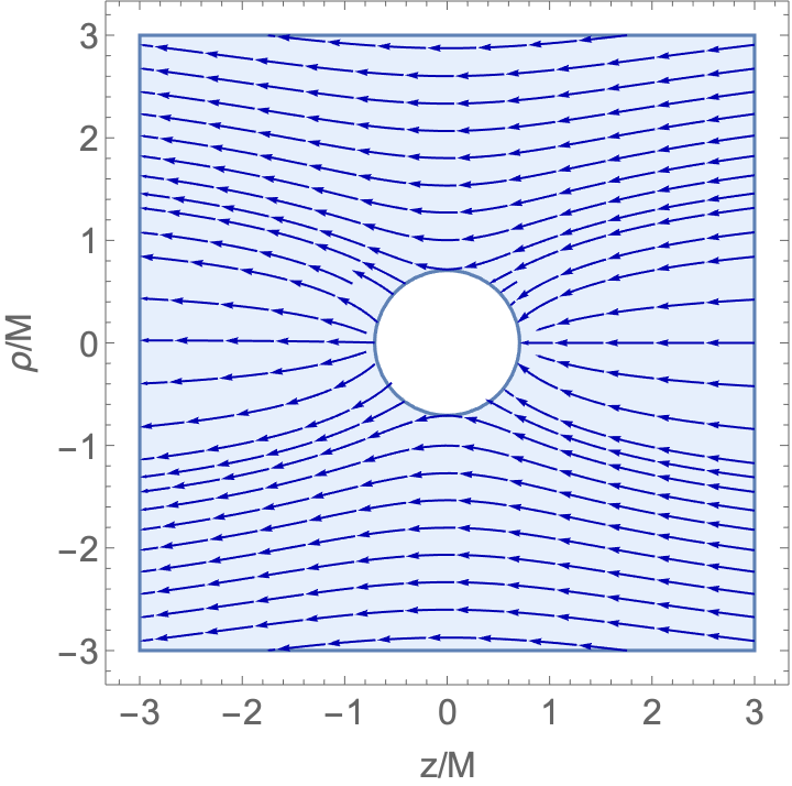
Figure 1: Magnetic field lines around black hole  in isotropic coordinates.

III.1.2 Source choice II

As the second choice of source, which turns out to be mathematically somewhat simpler, we use as our unperturbed solution the uniform magnetic field (and, for the case of perpendicular propagation, its companion electric field arising from the boost), corresponding to the flat space.

Thus, in this case the unperturbed potential for parallel propagation is

$$A^{(0)}_{\phi}=\frac{B_{0}\rho^{2}}{2}.$$ (34)

As a result, for our choice of the velocity, Eq. (23), the 1-form $u^{\mu}F^{(0)}_{\mu\nu}$ vanishes, so the source term now comes only from the left hand side of (2), i.e., from the vacuum Maxwell term. (This is not the case for perpendicular propagation, where both sides contribute to the source.)

The main advantage of this choice is that the relations are generally simpler. The second choice also highlights an important point: parameter $\kappa$ does not appear simply as an expansion parameter.

III.2 Main calculations: parallel propagation

For parallel propagation, it is convenient to use the cylindrical version of the isotropic coordinates, in which the metric has the form (II.3). The source then has only the azimuthal component, with the different choices discussed above corresponding to (see Appendix A for a collection of relevant mathematical relations)

$$S^{\phi}=MB_{0}\left\{\begin{array}[]{cc}\frac{\rho\left(2z^{2}-\rho^{2}\right)}{\left(\rho^{2}+z^{2}\right)^{5/2}}\times\beta^{2}\gamma^{2}\kappa,&\mbox{Choice I}\\ 2\partial_{\rho}\frac{1}{(\rho^{2}+z^{2})^{1/2}},&\mbox{Choice II}\end{array}\right.$$ (35)

As a consequence of our gauge choice, this source will produce a nontrivial deformation of $A_{\phi}$ only, $A^{(1)}_{\phi}(\rho,z)$, which is axially symmetric, and the equation for which can be brought to the Bessel form by the substitution

$$A^{(1)}_{\phi}(\rho,z)=\rho a(\rho,z)\,.$$ (36)

The equation becomes

$$\partial_{\rho}^{2}a+\frac{1}{\rho}\partial_{\rho}a-\frac{a}{\rho^{2}}+\Lambda^{2}\partial_{z}^{2}a=S^{\phi}\,.$$ (37)

This should be solved together with the regularity condition $A_{\phi}=0$ at $\rho=0$.

Going over to the Fourier transform with respect to $z$,

$$\tilde{a}(\rho,k_{z})=\int_{-\infty}^{\infty}dze^{-ik_{z}z}a(\rho,z)\,,$$

we obtain the equation

$$\partial_{\rho}^{2}\tilde{a}+\frac{1}{\rho}\partial_{\rho}\tilde{a}-\frac{\tilde{a}}{\rho^{2}}-\Lambda^{2}k^{2}\tilde{a}=-MB_{0}k\left\{\begin{array}[]{cc}2\left(1-\Lambda^{2}\right)\rho K_{0}\left(\rho k\right)&\mbox{Choice I}\\ 4K_{1}(k\rho),&\mbox{Choice II}\end{array}\right.$$ (38)

where $K_{0,1}$ are the modified Bessel functions, and $k\equiv|k_{z}|$. It is clear that this has a particular solution proportional to $K_{1}(k\rho)$; that solution, however, is singular at $\rho\to 0$. We must add to it the solution to the corresponding homogeneous equation, chosen so as to remove the singularity. The result is

$$\tilde{a}(\rho,k_{z})=\frac{MB_{0}}{k}\times\left\{\begin{array}[]{cc}\frac{4\Lambda K_{1}(\Lambda k\rho)}{1-\Lambda^{2}}-\frac{4K_{1}(k\rho)}{1-\Lambda^{2}}-2k\rho K_{0}(k\rho),&\mbox{Choice I}\\ \frac{4\Lambda K_{1}(\Lambda k\rho)}{1-\Lambda^{2}}-\frac{4}{1-\Lambda^{2}}K_{1}(k\rho),&\mbox{Choice II}\end{array}\right.$$ (39)

Recall that, upon multiplication by $\rho$ and the inverse Fourier transform, this has to be added to the corresponding zeroth-order term $A^{(0)}$, to produce the full vector potential to the required order. $A^{(0)}$, however, does not bring in any $\Lambda$ dependence. As a result, the Cherenkov terms $\propto K_{1}(\Lambda k\rho)$ must coincide for the two choices in (39), and we see that they indeed do.

The magnitude of (39) for Choice I is plotted, for different values of $\Lambda$ in Fig. 2. The special solution for $\Lambda=0$, the borderline between the regular and Cherenkov regimes, is

$$\tilde{a}\propto\frac{4}{\rho_{1}}-2\rho_{1}K_{2}$$ (40)

For small values of $\rho_{1}$, this goes as $\tilde{a}\propto\rho_{1}$; for $\rho_{1}\gg 1$ it decays as a power-law, $\tilde{a}\propto 4/\rho_{1}$.

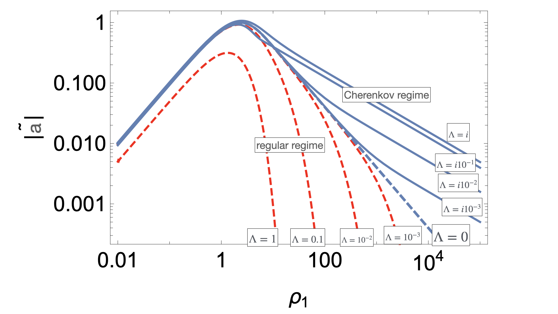
Figure 2: Vector potential $|\tilde{a}|$, Eq. (39), Choice I. The $\Lambda=0$ curve is given by (40) - it clearly serves as a separatrix between regular and Cherenkov regimes.

Its nature of the solution is different in the normal regime (real $\Lambda$) and the Cherenkov regime (complex $\Lambda$). We focus on the term involving $K_{1}(\Lambda k\rho)$. In the normal regime, $\Lambda^{2}>0$, at large distances, this term is fast decreasing:

$$\tilde{a}\propto\frac{e^{-\Lambda k\rho}}{(k\rho)^{1/2}}$$ (41)

In contrast, in the Cherenkov regime, $\Lambda^{2}<0$,

$$|\tilde{a}|\propto\frac{e^{\pm i|\Lambda|k\rho}}{\sqrt{k\rho}}$$ (42)

(We will return to the choice of the sign in this expression shortly.)

The solution (42) shows an oscillatory behavior, with decreasing amplitude $\propto\rho^{-1/2}$, characteristic of the cylindrical waves of Cherenkov radiation.

The term in $A^{(1)}_{\phi}$ responsible for radiation in the Cherenkov regime is then

$$A_{\phi}=\frac{4\Lambda}{1-\Lambda^{2}}\times\frac{MB_{0}}{k}\rho K_{1}(\Lambda k\rho)$$ (43)

where $\Lambda\to\pm i|\Lambda|$.

It is also instructive to compare the effect of the remaining (non-Cherenkov) terms in (39) for our two different choices of the source. We will do that by going over to the real space in the non-Cherenkov regime $\Lambda^{2}>0$. For Choice II, upon multiplication by $\rho$ and the Fourier transform to the coordinate space, we obtain

$$A^{(1)}_{\phi}(\rho,z)=\frac{2MB_{0}}{1-\Lambda^{2}}\left[(\rho^{2}+z^{2})^{1/2}-(\Lambda^{2}\rho^{2}+z^{2})^{1/2}\right]\,.$$ (44)

Observe that in the absence of the medium, i.e., for $\Lambda\to 0$, when expanded to the first order in $M$, (44) becomes

$$A_{\phi}(\rho,z)\approx\frac{1}{2}B_{0}\rho^{2}+\frac{MB_{0}\rho^{2}}{(\rho^{2}+z^{2})^{1/2}}\,.$$ (45)

The second (correction) term in this expression is precisely reproduced by the $\Lambda\to 1$ limit of the exact solution (32). Thus, the same term that is included as a part of the zeroth-order approximation for Choice I, appears as a part of the first-order solution for Choice II.

III.3 Emitted power

Given the vector potential in the Cherenkov regime (43) one can find the magnetic field in the BH frame, using the expressions $B_{z}=(1/\rho)\partial_{\rho}A_{\phi}$ and $B_{\rho}=-(ik_{z}/\rho)A_{\phi}$. After the boost along $z$ to the lab frame, the radial component $B_{\rho}$ gives rise to a tangential component of the electric field $E_{t}^{\prime}=-\gamma vB_{\rho}$. In addition, we need to replace $z$ with $z=\gamma(z^{\prime}-vt^{\prime})$ in the formulas of the inverse Fourier transform as, for instance, in

$$E_{t}^{\prime}=-\gamma v\int_{-\infty}^{\infty}\frac{dk_{z}}{2\pi}e^{ik_{z}\gamma(z^{\prime}-vt^{\prime})}B_{\rho}\,.$$ (46)

The total power radiated in the Cherenkov regime through a cylindrical surface at a large $\rho$ is given by

$${\cal P}=\frac{1}{4\pi}2\pi\rho\int_{-\infty}^{\infty}dz^{\prime}E_{t}^{\prime}B_{z}^{\prime}=-\frac{1}{2}v\rho\int_{-\infty}^{\infty}\frac{dk_{z}}{2\pi}B_{\rho}B_{z}^{*}\,.$$ (47)

(Note the disappearance of $\gamma$ in the last expression.) Here, it is sufficient to use the slowly decaying radiation parts of the fields, obtained by an analytical continuation to imaginary $\Lambda$. Eq. (46) shows that this continuation should be carried out differently, depending on the sign of $k_{z}$. Indeed, for $k_{z}>0$, the frequency

$$\omega^{\prime}=\gamma k_{z}v$$

in (46) is positive, so that the outgoing cylindrical wave is given by the Hankel function $H^{(1)}(|\Lambda|k\rho)$, which is obtained via

$$\Lambda=-i|\Lambda|\,.$$

For $k_{z}<0$, the frequency is negative, and the outgoing wave is $H^{(2)}(|\Lambda|k\rho)$, corresponding to $\Lambda=i|\Lambda|$. As a result, the Fourier transforms of the radiation fields required by (47) are

$$B_{\rho} = -\frac{4MB_{0}|\Lambda|}{1+|\Lambda|^{2}}K_{1}(\mp i|\Lambda|k\rho)\,,\mbox{}$$

$$\mbox{}B_{z} = \frac{4MB_{0}|\Lambda|^{2}}{1+|\Lambda|^{2}}K_{0}(\mp i|\Lambda|k\rho)\,,$$ (48)

where the upper sign corresponds to $k_{z}>0$, and the lower to $k_{z}<0$.

Substituting (48) in (47) and using the large-argument asymptotics of the Bessel functions, we obtain

$${\cal P}_{\parallel}=2\beta\left(\frac{MB_{0}|\Lambda|}{1+|\Lambda|^{2}}\right)^{2}\int_{-\infty}^{\infty}\frac{dk_{z}}{k}$$ (49)

Estimating maximal $k_{z}\sim 1/R_{g}$ and minimal $k_{z}\sim 1/R_{s}$, the size of the system, we obtain the total luminosity as

$${\cal P}_{\parallel}\approx\frac{\beta|\Lambda|^{2}}{\left(1+|\Lambda|^{2}\right)^{2}}\times(B_{0}R_{g})^{2}c\times\log\left(\frac{R_{s}}{R_{g}}\right)$$ (50)

where we reinstated dimensional quantities.

IV Motion across magnetic field

IV.1 The source

Next we consider the case of BH moving across magnetic field. This case turns out to be somewhat mathematically more complicated than the motion along the magnetic field, since there is no cyclic coordinate.

In the black hole frame there are now crossed electric and magnetic fields at infinity. We chose the velocity of the black hole along $z$ and the asymptotic magnetic field along $x$, so that the asymptotic electric field is along $-y$. The isotropic Cartesian coordinates all have the same diagonal elements, equal to $g_{zz}$ in Eq. (II.3).

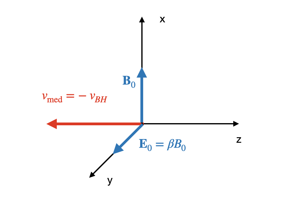
Figure 3: Choice of coordinates for black hole moving perpendicular to magnetic field. In the frame of black hole the medium is moving with velocity $-v_{\rm BH}$ (along $-z$), producing crossed magnetic and electric fields at infinity.

Similarly to the case of parallel propagation, we have freedom in choosing the zeroth-order state. The Choice-I is to start with gravity-distorted fields, so that in the black hole frame, the four-potential for constant electromagnetic fields in the symmetric gauge is (note new notation for the fields)

$$A=\left\{1,0,0,0\right\}\left(1-\frac{M}{2r}\right)^{2}y{\cal E}_{0}+\mbox{}$$

$$+\left\{0,0,-z/2,y/2\right\}\left(1+\frac{M}{2r}\right)^{4}{\cal B}_{0}\mbox{}$$

$${\cal E}_{0}=\beta\gamma B_{0}\mbox{}$$

$${\cal B}_{0}=\gamma B_{0}\mbox{}$$

$$r=\sqrt{\rho^{2}+z^{2}}\mbox{}$$

$$\rho^{2}=x^{2}+y^{2}$$ (51)

where $B_{0}$ is the magnetic field in the lab frame, and ${\cal E}_{0}$, ${\cal B}_{0}$ are the asymptotic values of the electric and magnetic fields in the BH frame.

Alternatively, we can treat the distortion as a part of the fluctuating field. In this Choice-II the unperturbed state is

$$A=\left\{y\beta,0,-z/2,y/2\right\}{\cal B}_{0}\,.$$ (52)

We have already demonstrated that for parallel propagation the two choices result in the same radiative term. As it turns out, computations for the choice (52) are somewhat simpler, so we proceed with it here. For reference, the sources corresponding to (51) are given in Appendix B.

In this section, we choose the 4-velocity of the medium in the form (25). The corresponding expressions for a more general (one-parameter) choice are given in Appendix C.

We find the first-order sources for equation (26) (in the $t,x,y,z$ coordinates) as

$$S^{\rho}=\left(\begin{array}[]{c}-\frac{2\beta\rho\left(1+\gamma^{2}\kappa\right)\sin\phi}{\left(\rho^{2}+z^{2}\right)^{3/2}}\\ 0\\ \frac{2\Lambda^{2}z}{\left(\rho^{2}+z^{2}\right)^{3/2}}\\ -\frac{2\Lambda^{2}\rho\sin\phi}{\left(\rho^{2}+z^{2}\right)^{3/2}}\\ \end{array}\right)\times{\cal B}_{0}M$$ (53)

where ${\cal B}_{0}=\gamma B_{0}$ is the magnetic field in the BH frame, and $\phi$ is the azimuthal angle. (Component $S_{x}=0$ is due to interference of E-produced and B-produced terms, each is non-zero independently.)

The Fourier transform in $z$ gives

$$S^{\rho}=\left(\begin{array}[]{c}-4\beta\left(1+\gamma^{2}\kappa\right)kK_{1}\left(\rho k\right)\sin\phi\\ 0\\ -4i\Lambda^{2}k_{z}K_{0}\left(\rho k\right)\\ -4\Lambda^{2}kK_{1}\left(\rho k\right)\sin\phi\\ \end{array}\right)\times{\cal B}_{0}M$$ (54)

The $0$ and $z$ components of this can be combined according to (28),

$$\left(\begin{array}[]{c}S_{1}\\ S_{2}\\ \end{array}\right)=-\left(\begin{array}[]{c}\frac{2+\kappa}{1+\kappa}\beta\\ 1+\beta^{2}\\ \end{array}\right)\times 4{\cal B}_{0}MkK_{1}\left(\rho k\right)\sin\phi$$ (55)

for use in the general equation (30).

IV.2 Fluctuating components and Poynting power for perpendicular propagation

Calculations of emission for perpendicular case mostly follow the procedures described in §III.2 and §III.3. There are a few new effects, though.

For perpendicular propagation the source separates into three parts : $S_{y}$, $S_{0}$ and $S_{z}$. Each component will produce correspondingly three fluctuating potenetials $A_{y}$, $A_{0}$ and $A_{z}$. In the BH frame the corresponding electromagnetic fields are stationary. Boosting to the lab frame, we then obtain propagating waves. Importantly, even though each fluctuating component can be calculated independently, the resulting Poynting flux includes also cross-terms.

The y-component of the general equation (30) with the source from (54) has a solution

$$A_{y}=-\frac{4i}{k_{z}}\left[K_{0}\left(\rho_{1}\right)-K_{0}\left(\Lambda\rho_{1}\right)\right]\times\frac{\Lambda^{2}}{1-\Lambda^{2}}\times{\cal B}_{0}M$$ (56)

where $\rho_{1}=k\rho$.

The radiative part of (56) is

$$A_{y}^{(rad)}=\frac{4i\Lambda^{2}K_{0}\left(\Lambda\rho_{1}\right)}{k_{z}\left(1-\Lambda^{2}\right)}\times{\cal B}_{0}M$$ (57)

For the $A_{0}-A_{z}$ components, using sources (54) and fluctuating fields combined according to (28), we find

$$A_{1}=\frac{\beta(2+\kappa)}{(1+\kappa)\left(1-\Lambda^{2}\right)}\left[\Lambda K_{1}\left(\Lambda\rho_{1}\right)-K_{1}\left(\rho_{1}\right)\right]\times\frac{4{\cal B}_{0}M\sin\phi}{k}\mbox{}$$

$$A_{2}=\frac{1+\beta^{2}}{1-\Lambda^{2}}\left[K_{1}\left(\rho_{1}\right)-\Lambda K_{1}\left(\Lambda\rho_{1}\right)\right]\times\frac{4{\cal B}_{0}M\sin\phi}{k}$$ (58)

These can be combined to form $A_{0,z}$ according to (28),

$$A_{0}=-\frac{\beta}{1+\kappa}\frac{\Lambda^{2}}{1-\Lambda^{2}}\left[\Lambda K_{1}\left(\Lambda\rho_{1}\right)-K_{1}\left(\rho_{1}\right)\right]\times\frac{4{\cal B}_{0}M\sin\phi}{k}\mbox{}$$

$$A_{z}=\frac{1+\gamma^{2}\kappa}{(1+\kappa)\left(1-\Lambda^{2}\right)}\left[\Lambda K_{1}\left(\Lambda\rho_{1}\right)-K_{1}\left(\rho_{1}\right)\right]\times\frac{4{\cal B}_{0}M\sin\phi}{k}$$ (59)

It may be verified that the vector $\{A_{0},0,A_{y},A_{z}\}$ satisfies the gauge condition (13).

We can write for the radiative part $\propto K_{0,1}\left(\Lambda\rho k_{z}\right)$

$$A^{(rad)}=\left\{c_{0}K_{1}\left(x\right)\sin(\phi),0,\frac{ik_{z}c_{y}}{k}K_{0}\left(x\right),c_{z}K_{1}\left(x\right)\sin(\phi)\right\}\times\frac{M{\cal B}_{0}}{k}\mbox{}$$

$$x=\Lambda k\rho\mbox{}$$

$$c_{0}=-\frac{4\beta\Lambda^{3}}{(1+\kappa)\left(1-\Lambda^{2}\right)}\mbox{}$$

$$c_{y}=\frac{4\Lambda^{2}}{1-\Lambda^{2}}\mbox{}$$

$$c_{z}=\frac{4\Lambda\left(\gamma^{2}\kappa+1\right)}{(1+\kappa)\left(1-\Lambda^{2}\right)}$$ (60)

Gauge condition ensures that

$$c_{0}=\frac{\beta\Lambda\left(c_{y}-\Lambda c_{z}\right)}{1-\Lambda^{2}}$$ (61)

At large $\rho$, we can use the asymptotic form of the Bessel functions

$$K_{n}(x)\to\sqrt{\pi/(2x)}e^{-x}\equiv f(x)$$ (62)

The radiative part of the 4-potential is then

$$A^{(rad)}=\{c_{0}\sin\phi,0,\frac{ik_{z}c_{y}}{k},c_{z}\sin\phi\}\frac{f(x)}{k}$$ (63)

The electric and magnetic fields in the BH frame, in the cylindrical coordinates $(\rho,\phi,z)$, become

$${\bf E}=\left\{-\Lambda,0,\frac{ik_{z}}{k}\right\}\times c_{0}\sin\phi\times f(x)\times M{\cal B}_{0}\mbox{}$$

$${\bf B}=\left\{c_{y}\cos(\phi),\frac{c_{0}\left(\Lambda^{2}-1\right)\sin(\phi)}{\beta\Lambda},-\frac{ik_{z}\Lambda c_{y}}{k}\cos(\phi)\right\}\times f(x)\times M{\cal B}_{0}$$ (64)

To obtain the power radiated in the Cherenkov regime, we follow the same procedure as in the case of parallel propagation. Namely, we boost these expressions to the lab frame and analytically continue the results via $\Lambda\to\pm i|\Lambda|$, with the sign depending again on the sign of $k_{z}$.

For the radial Poynting vector we find

$${F}_{\rho}=\left(c_{y}^{2}\cos^{2}(\phi)+\frac{|c_{0}|^{2}(1+\kappa)\sin^{2}(\phi)}{|\Lambda|^{2}}\right)\times\frac{\beta\gamma}{8\rho k}\times(\gamma MB_{0})^{2}$$ (65)

where we eliminated $c_{z}$ according to (61) to demonstrate that the Poynting flux at infinity is explicitly positive.

Finally the Cherenkov power for perpendicular propagation reduces to a relatively compact expression

$${\cal P}_{\perp}=2\beta\times\left(\frac{|\Lambda|^{2}}{1+|\Lambda|^{2}}\right)^{2}\times\left(\cos^{2}(\phi)+\frac{\beta^{2}\sin^{2}(\phi)}{\epsilon}\right)\times\frac{dk}{2\pi k}\times(\gamma MB_{0})^{2}\mbox{}$$

$${\cal P}_{\perp,tot}=\int{\cal P}_{\perp}d\phi=\beta\left(1+\beta^{2}/\epsilon\right)\left(\frac{|\Lambda|^{2}}{1+|\Lambda|^{2}}\right)^{2}\times\frac{dk}{k}\times(\gamma MB_{0})^{2}$$ (66)

(compare with the parallel case (49)).

We may also perform inverse Fourier transforms to find fields in coordinate space

$$A_{y}(z,\rho)=\frac{\Lambda^{2}}{1-\Lambda^{2}}\ln\left(\frac{\Lambda\left(\sqrt{\rho^{2}+z^{2}}+z\right)}{\sqrt{\Lambda^{2}\rho^{2}+z^{2}}+z}\right)\times 2\gamma MB_{0}\mbox{}$$

$$A_{0}(z,\rho)=\beta\frac{\Lambda^{2}}{\epsilon\left(1-\Lambda^{2}\right)}\left(\sqrt{\rho^{2}+z^{2}}-\sqrt{\Lambda^{2}\rho^{2}+z^{2}}\right)\times\frac{2\gamma MB_{0}\sin\phi}{\rho}\mbox{}$$

$$A_{z}=-\frac{1+\gamma^{2}\kappa}{\beta\Lambda^{2}}A_{0}$$ (67)

(Cherenkov condition is not assumed in (67).)

V Observability

A simple order-of-magnitude estimate of Cherenkov power is given by Eqns. (50) and (66). Returning to dimensional quantities

$$L\sim\beta_{K}B(r)^{2}\left(\frac{2GM_{BH}}{c^{2}}\right)^{2}c\Lambda_{c}\mbox{}$$

$$B(r)\approx B_{NS}\left(\frac{r}{R_{NS}}\right)^{-3}\mbox{}$$

$$\beta_{K}\sim\sqrt{\frac{GM_{tot}}{rc^{2}}}\mbox{}$$

$$\Lambda_{c}=\ln\frac{k_{max}}{k_{min}}$$ (68)

($B(r)$ is the magnetic field at distance $r$ expressed in term of the surface magnetic field, $\beta_{K}$ is the beta-parameter for Keplerian motion, $M_{tot}$ is the total mass of the system, and $\Lambda_{c}$ is a parameter similar to Coulomb logarithm).

Consider first a merger of a stellar mass BH $M_{BH}\geq$ few $\times M_{\odot}\gg M_{NS}$ (so that $M_{tot}\sim M_{BH}$) merging with a neutron star of surface magnetic field $B_{NS}$.

Using time to merger in post-Newtonian approximation Cutler and Flanagan (1994)

$$-t=\frac{5}{256}\frac{c^{5}}{G^{3}}\frac{r^{4}}{M_{1}M_{2}M_{tot}},$$ (69)

(estimate of $-t$ is valid approximately to $-t\sim$ milliseconds), we find

$$L_{\rm BH,10M_{\odot}}\approx 4B_{NS}^{2}\frac{(GM_{BH})^{2}(GM_{tot})^{1/2}R_{{NS}}^{6}}{c^{4}r^{13/2}}\Lambda_{c}\approx 10^{38}\,{\rm erg\,s}^{-1}(-t)^{-13/8}\left(\frac{B_{NS}}{10^{12}{\rm G}}\right)^{2}\left(\frac{M_{BH}}{10M_{\odot}}\right)^{-3/4}$$ (70)

where $-t$ is time to merger in seconds, we assumed that the total mass is dominated by the BH, and approximated $\Lambda_{c}\sim\ln R_{NS}/(2GM_{BH}/c^{2})\approx 1$. The peak power, estimated at $-t\sim$ millisecond is $\sim$ few $10^{42}$ erg s^-1. (Incidentally, the value of peak power comes close to the parameters of enigmatic Fast Radio Bursts Cordes and Chatterjee (2019), but the expected corresponding rates naturally do not match.)

On the one hand, the peak luminosity is not high, similar to other mechanisms based on unipolar inductor scaling (Hansen and Lyutikov, 2001; Lyutikov, 2011b). But it can be detectable in radio - the corresponding peak flux is in the kilo Janskys range if coming from $\sim 100$ Mpc distance Lyutikov (2024).

An important constraint comes from the expansion in small mass of the BH, which translates to the requirement that the emitted wavelength should be larger than the Schwarzschild radius. For stellar mass BHs the Schwarzschild radius is kilometers, this implies frequencies below the kilo-Hertz range. Depending on the parameters at the source, such low frequencies may not be able to propagate due to plasma cut-off at $\omega=\omega_{p}$. The required density is $\leq 1$ cm^-3. This is somewhat larger than the typical density in the volume-dominant warm phase of ISM ($n_{ISM}\sim 10^{-2}-10^{-1}$ cm^-3).

Primordial black holes (Carr et al., 2021) may not suffer from such limitation - their emitted frequency can be in the GHz range for masses $M_{BH}\sim 10^{-6}M_{\odot}$. The corresponding power for a primordial black hole flying through the magnetosphere of a neutron star can be estimated using (68) with $B\sim B_{NS}$ and $\Lambda_{c}\sim\ln R_{NS}/(2GM_{BH}/c^{2})\approx 15$. We find

$$L_{\rm BH,10^{-6}M_{\odot},max}\approx 4\times 10^{34}\,{\rm erg\,s}^{-1}$$ (71)

VI Discussion

We discuss a novel effect at the intersection of general relativity, electromagnetism, and the physics of continuous media: Cherenkov emission by an uncharged superluminally moving Schwarzschildblack hole. Interestingly, in this case there are no source terms: emission originates as a perturbation-of-a-perturbation: the initial electromagneticfields are distorted by gravity, and in the Cherenkov regime the perturbations of those distorted fields propagate as electromagnetic waves.

In the Cherenkov regime, emission conditions involve the combination

$$|\Lambda|B_{0}M\equiv\sqrt{|\beta^{2}\gamma^{2}\kappa-1|}B_{0}(GM)$$ (72)

(see Appendix §C for an interesting exception).

Scaling (72) indicates that the effect is the interplay between gravity $(GM)$, magnetic field $B_{0}$, and physics of movement of continuous media $\Lambda$: $\kappa\neq 0$, $\beta\neq 0$ is needed, plus the Cherenkov condition.

The process involves an number of subtle physical effects:

• In Cherenkov emission, it is the medium that emits. Conventionally, a moving particle produces an electromagnetic perturbation - these perturbations force the particles of the medium to emit coherently in the Cherenkov regime. In our case, it is the gravity of the black hole that “shakes” the particles of the medium.

• Gravity propagates with the speed of light, but the corresponding disturbances electromagnetic are delayed. This leads to a fairly complicated effective source structure.

• Important simplification is achieved by transforming to the black hole frame. Our approach for treating fluctuations follows the conventional Cherenkov case. In this frame, all fields are stationary.

• The emitted spectrum is red-dominated $\propto dk_{z}/|k_{z}|$. Formally, the lowest emitted frequency is then determined by the size of the system, but for low frequencies, our assumptions will be violated (e.g., plasma cut-off effects).

An important free ingredient in the model is the choice of the velocity field, as we do not solve for the motion of matter. The results in general depend on that choice. In particular, there is one special case when there is no Cherenkov emission. It occurs for a black hole propagating along the direction of the magnetic field  at infinity in the regime when locally the matter flows along the magnetic field.

Note also that one cannot gain much in a highly dielectric medium with $\epsilon\gg 1$ (possibly large values of $\Lambda$) since Cherenkov powers (50) and (66) typically level off as functions of $\Lambda$.

We thank Roger Blandford and Ilya Mandel for discussions and comments on the manuscript.

Appendix A Relevant mathematical formulae

In many cases we deal with equation

$$\Delta_{\perp}f-\Lambda^{2}f=S\mbox{}$$

$$S=Z(\rho_{1})e^{im\phi}$$ (73)

with $m=0,\,1$; $Z$ is a Bessel function of orders $0$ or $1$, $\rho_{1}$ is dimensionless cylindrical coordinate.

The homogeneous equation, $S=0$,

$$\Delta_{\perp}f-\Lambda^{2}f=0$$ (74)

has solutions

$$f=K_{0}(\Lambda{\rho_{1}})\mbox{}$$

$$f=K_{1}(\Lambda{\rho_{1}})e^{i\phi}$$ (75)

The following are relevant solutions of the inhomogeneous equation (it appears that the following relations are not listed in the standard textbooks on Bessel functions)

$$S=K_{0}(\rho_{1})\to f=\frac{1}{1-\Lambda^{2}}K_{0}(\rho_{1})\mbox{}$$

$$S=\rho_{1}K_{1}(\rho_{1})\to f=\left(\rho_{1}K_{1}\left(\rho_{1}\right)+\frac{2K_{0}\left(\rho_{1}\right)}{1-\Lambda^{2}}\right)\frac{1}{1-\Lambda^{2}}\mbox{}$$

$$S=K_{1}(\rho_{1})e^{i\phi}\to f=\frac{1}{1-\Lambda^{2}}K_{1}(\rho_{1})e^{i\phi}\mbox{}$$

$$S=\rho_{1}K_{0}(\rho_{1})e^{i\phi}\to f=\left({\rho_{1}K_{0}\left(\rho_{1}\right)}+\frac{2K_{1}\left(\rho_{1}\right)}{\left(1-\Lambda^{2}\right)}\right)\frac{e^{i\phi}}{1-\Lambda^{2}}$$ (76)

The following combinations of the homogeneous and inhomogeneous solutions are well-behaving at $\rho_{1}\to 0$

$$S=K_{0}(\rho_{1})\to f=\frac{1}{1-\Lambda^{2}}\left(K_{0}(\rho_{1})-K_{0}(\Lambda\rho_{1})\right)\mbox{}$$

$$S=\rho_{1}K_{1}(\rho_{1})\to f=\left(\frac{2K_{0}\left(\rho_{1}\right)}{1-\Lambda^{2}}-\frac{2K_{0}\left(\Lambda\rho_{1}\right)}{1-\Lambda^{2}}+\rho_{1}K_{1}\left(\rho_{1}\right)\right)\frac{1}{1-\Lambda^{2}}\mbox{}$$

$$S=K_{1}(\rho_{1})e^{i\phi}tof=\left(K_{1}(\rho_{1})-\Lambda K_{1}(\Lambda\rho_{1})\right)\frac{e^{i\phi}}{1-\Lambda^{2}}\mbox{}$$

$$S=\rho_{1}K_{0}(\rho_{1})e^{i\phi}\to f=\left(\rho_{1}K_{0}\left(\rho_{1}\right)+\frac{2\left(K_{1}\left(\rho_{1}\right)-\Lambda K_{1}\left(\Lambda\rho_{1}\right)\right)}{1-\Lambda^{2}}\right)\frac{e^{i\phi}}{1-\Lambda^{2}}$$ (77)

The radiation components correspond to terms dependent on $(\Lambda\rho_{1})$.

The importance of these relations is: perturbation theory may start with different assumptions about the zeroth-order state. For example, we may chose flat metric and treat effects of gravity and of the medium as perturbations, or we may chose vacuum solutions in curved space, and add matter effects. Different choices of the zeroth-order state result in different sources $S$, but in the same radiation components.

Appendix B Sources for perpendicular motion with initial state (51)

Perturbations of both the electric field and magnetic field will each produce Cherenkov-like emission (in some cases adding destructively).

Following the procedure described above, we find the total source

$$S^{0}=-\left(\frac{3\beta^{2}\gamma^{2}\rho^{2}}{\left(\rho^{2}+z^{2}\right)^{5/2}}+\frac{2}{\left(\rho^{2}+z^{2}\right)^{3/2}}\right)\beta\rho\sin\phi\times\kappa{\cal B}_{0}M\mbox{}$$

$$S^{x}=0\mbox{}$$

$$S^{y}=\frac{z\left(2z^{2}-\rho^{2}\right)}{\left(\rho^{2}+z^{2}\right)^{5/2}}\beta^{2}\gamma^{2}\times\kappa{\cal B}_{0}M\mbox{}$$

$$S^{z}=\frac{\rho\left(\rho^{2}+4z^{2}\right)}{\left(\rho^{2}+z^{2}\right)^{5/2}}\beta^{2}\gamma^{2}\sin\phi\times\kappa{\cal B}_{0}M$$ (78)

where we used $y=\rho\sin\phi$. (Component $S_{x}=0$ is due to interference of E-produced and B-produced terms, each is non-zero independently).

The Fourier transform of the source is

$$S^{0}=-2k_{z}^{2}\beta\left(\beta^{2}\gamma^{2}\rho_{1}K_{2}(\rho_{1})+2K_{1}(\rho_{1})\right)\sin\phi\times\cos\left(k_{z}z\right)\times\beta{\cal B}_{0}\kappa M\mbox{}$$

$$S^{x}=0\mbox{}$$

$$S^{y}=2\beta^{2}\gamma^{2}k_{z}\left(\rho_{1}K_{1}(\rho_{1})-2K_{0}(\rho_{1})\right)\times\sin\left(k_{z}z\right)\times\beta{\cal B}_{0}\kappa M\mbox{}$$

$$S^{z}=2\beta^{2}\gamma^{2}k_{z}^{2}\left(4K_{1}(\rho_{1})-\rho_{1}K_{2}(\rho_{1})\right)\sin\phi\times\cos\left(k_{z}z\right)\times\beta{\cal B}_{0}\kappa M$$ (79)

Explicit sine and cosine transforms are indicated, and overall normalization $\times{\cal G}$ has been omitted. We also explicitly give the source for the $0-z$ combination. (The $S_{y}$ source is weakly divergent at $\rho_{1}\to 0$ as $\ln\rho_{1}$.)

Appendix C Choices of velocity field for perpendicular propagation

For perpendicular propagation, unlike the case of motion parallel to the field, there is no longer a universal result for arbitrary “straight-line” motion. In other words, the result depends on the form of the coordinate dependence in

$$u^{\mu}=[u^{0}({\bf x}),0,0,u^{z}({\bf x})]$$

Here, we consider expressions for the 4-velocity that are of the form

$$u^{\mu}=[\gamma(1+a/r),0,0,-\gamma\beta(1+b/r)]$$

where the constants $a$ and $b$ are $O(M)$, chosen so that the condition $u^{2}=-1$ is satisfied to the first order in $M$. The condition $u^{2}=-1$ results in the relation

$$M-a+\beta^{2}(M+b)=0$$

To the zeroth order, i.e., for $u^{\mu}_{(0)}=(\gamma,0,0,-\gamma\beta)$ in the BH frame, the condition $u^{\mu}_{(0)}F^{(0)}_{\mu\nu}$ holds:

$$\gamma F^{(0)}_{0y}-\gamma\beta F^{(0)}_{zy}=0$$

where

$$F^{(0)}_{0y}=-\gamma\beta B_{0}\,,\hskip 30.00005ptF^{(0)}_{zy}=-\gamma B_{0}\,,$$

are obtained as a result of the Lorentz transformation of the magnetic field to the BH frame. To the first order, however,

$$u^{\mu}F^{(0)}_{\mu y}\approx(b-a)\gamma^{2}\beta MB_{0}\frac{1}{r}=-2CM\beta B_{0}\frac{1}{r}$$

where we have defined

$$C\equiv\frac{1}{2M}\gamma^{2}(a-b)$$

Unless $a=b$, this is nonzero, meaning that the right-hand side of (2) now contributes to the source. The model used in the main text corresponds to $a=-b=M$, and $C=\gamma^{2}$.

The components of the source $S^{\alpha}\equiv-[L_{1}A^{(0)}]^{\alpha}$ in (15) are now obtained, in parallel with those for the parallel motion as

$$S^{0} = -\partial_{y}(\sqrt{-g}g^{yy}g^{00}F^{(0)}_{y0})-\kappa\gamma\partial_{y}(u^{\mu}F^{(0)}_{\mu y})\approx 2M\gamma vB_{0}(1+C\kappa)\partial_{y}\frac{1}{r}\,,$$ (80)

$$S^{x} = 0\,,$$ (81)

$$S^{y} = -\partial_{z}(\sqrt{-g}g^{zz}g^{yy}F^{(0)}_{zy})-\kappa\gamma\beta\partial_{z}(u^{\mu}F^{(0)}_{\mu y})\approx-2M\gamma B_{0}(1-C\kappa\beta^{2})\partial_{z}\frac{1}{r}\,,$$ (82)

$$S^{z} = -\partial_{y}(\sqrt{-g}g^{yy}g^{zz}F^{(0)}_{yz})+\kappa\gamma\beta\partial_{y}(u^{\mu}F^{(0)}_{\mu y})\approx 2M\gamma B_{0}(1-C\kappa\beta^{2})\partial_{y}\frac{1}{r}\,,$$ (83)

where we have used the components of the metric correct to the first order in $M$.

Recall that these are the sources for $\Psi^{\mu}$, which is related to $A^{(1)}_{\mu}$ by Eq. (16):

$$A^{(1)}_{\nu}=\widetilde{\Pi}_{\nu\rho}\Psi^{\rho}\,.$$

The sources for $A^{(1)}_{\mu}$ then are

$$j_{\mu}=\widetilde{\Pi}_{\mu\nu}S^{\nu}$$

for which we find

$$j_{0}=C_{0}\partial_{y}\frac{1}{r},\hskip 30.00005ptj_{x}=0,\hskip 30.00005ptj_{y}=C_{y}\partial_{z}\frac{1}{r},\hskip 30.00005ptj_{z}=C_{z}\partial_{y}\frac{1}{r}$$

where

$$C_{0} = 2M\gamma B_{0}\beta\left[-(1+C\kappa)+\frac{2\kappa\gamma^{2}}{1+\kappa}+\frac{C\kappa^{2}}{1+\kappa}\right]$$ (84)

$$C_{y} = -2M\gamma B_{0}(1-C\kappa\beta^{2})$$ (85)

$$C_{z} = 2M\gamma B_{0}\left[1-C\kappa\beta^{2}+\frac{2\kappa\gamma^{2}\beta^{2}}{1+\kappa}+\frac{C\kappa^{2}\beta^{2}}{1+\kappa}\right]$$ (86)

There is a relation between the coefficients,

$$C_{y}+\kappa\gamma^{2}\beta C_{0}+\Lambda^{2}C_{z}=0\,,$$ (87)

which is a consequence of the gauge condition (13). Using this relation, we can bring the total power radiated in the Cherenkov regime through a cylindrical surface at a large $\rho$ to the form

$${\cal P}=\frac{\beta}{4(1+|\Lambda|^{2})^{2}}\left(C_{y}^{2}+\epsilon C_{0}^{2}\right)\int_{-\infty}^{\infty}\frac{dk_{z}}{k}\,,$$ (88)

where as before it is understood that the integral needs to be cut off both at small and at large wavenumbers.

A curious aspect of the formula (88) is that it shows that using a different model for the velocity than the one in the main text in general changes the threshold ($\Lambda\to 0$) behavior. Indeed, for the model in the text, $C_{y}$ and $C_{0}$ are both proportional to $|\Lambda|^{2}$, which results in an overall factor of $|\Lambda|^{4}$ in the power. We see, however, that this not the generic behavior: generically, the power sets in at a nonzero value immediately once the Cherenkov regime is reached. This is the behavior argued previously to occur for the Cherenkov radiation by a magnetic dipole moving superluminally in a medium and oriented perpendicular to the direction of motion (Frank, 1984)

References

- Blandford and Znajek (1977) R. D. Blandford and R. L. Znajek, MNRAS 179, 433 (1977).
- Palenzuela et al. (2010) C. Palenzuela, L. Lehner, and S. L. Liebling, Science 329, 927 (2010), eprint 1005.1067.
- Lyutikov (2011a) M. Lyutikov, Phys. Rev. D 83, 064001 (2011a), eprint 1101.0639.
- Lyutikov (2011b) M. Lyutikov, Phys. Rev. D 83, 124035 (2011b), eprint 1104.1091.
- Lyutikov and McKinney (2011) M. Lyutikov and J. C. McKinney, Phys. Rev. D 84, 084019 (2011), eprint 1109.0584.
- Bransgrove et al. (2021) A. Bransgrove, B. Ripperda, and A. Philippov, Phys. Rev. Lett. 127, 055101 (2021), eprint 2109.14620.
- Abbott et al. (2016) B. P. Abbott, R. Abbott, T. D. Abbott, M. R. Abernathy, F. Acernese, K. Ackley, C. Adams, T. Adams, P. Addesso, R. X. Adhikari, et al., Physical Review X 6, 041015 (2016), eprint 1606.04856.
- Abbott et al. (2017) B. P. Abbott, R. Abbott, T. D. Abbott, F. Acernese, K. Ackley, C. Adams, T. Adams, P. Addesso, R. X. Adhikari, V. B. Adya, et al., ApJ Lett. 848, L12 (2017), eprint 1710.05833.
- Lyutikov (2024) M. Lyutikov, arXiv e-prints arXiv:2402.16504 (2024), eprint 2402.16504.
- Hansen and Lyutikov (2001) B. M. S. Hansen and M. Lyutikov, MNRAS 322, 695 (2001), eprint astro-ph/0003218.
- Lyutikov (2019) M. Lyutikov, MNRAS 483, 2766 (2019).
- Most and Philippov (2020) E. R. Most and A. A. Philippov, ApJ Lett. 893, L6 (2020), eprint 2001.06037.
- Lyutikov (2023) M. Lyutikov, Phys. Rev. E 107, 025205 (2023), eprint 2211.14433.
- Auston et al. (1984) D. H. Auston, K. P. Cheung, J. A. Valdmanis, and D. A. Kleinman, Phys. Rev. Lett. 53, 1555 (1984).
- Barnard and Arons (1986) J. J. Barnard and J. Arons, Astrophys. J. 302, 138 (1986).
- Lyutikov (1999) M. Lyutikov, Journal of Plasma Physics 62, 65 (1999), eprint physics/9807022.
- Tamm and Frank (1937) I. E. Tamm and I. M. Frank, Soviet Physics - Doklady 14, 107 (1937).
- Jauch and Watson (1948a) J. M. Jauch and K. M. Watson, Physical Review 74, 950 (1948a).
- Jauch and Watson (1948b) J. M. Jauch and K. M. Watson, Physical Review 74, 1485 (1948b).
- Bolotovsky and Stolyarov (1974) B. M. Bolotovsky and C. N. Stolyarov, Physics Uspekhi 4, 569 (1974).
- Bolotovskii (1957) B. M. Bolotovskii, Usp. Fiz. Nauk 62, 201 (1957), URL https://ufn.ru/ru/articles/1957/7/a/.
- Clemmow (1974) P. C. Clemmow, Journal of Plasma Physics 12, 297 (1974).
- Landau and Lifshitz (1960) L. D. Landau and E. M. Lifshitz, Electrodynamics of continuous media (1960).
- Cutler and Flanagan (1994) C. Cutler and É. E. Flanagan, Phys. Rev. D 49, 2658 (1994), eprint gr-qc/9402014.
- Cordes and Chatterjee (2019) J. M. Cordes and S. Chatterjee, ARAA 57, 417 (2019), eprint 1906.05878.
- Carr et al. (2021) B. Carr, K. Kohri, Y. Sendouda, and J. Yokoyama, Reports on Progress in Physics 84, 116902 (2021), eprint 2002.12778.
- Frank (1984) I. M. Frank, Soviet Physics Uspekhi 27, 772 (1984).