When Machine Learning Gets Personal:
Understanding Fairness of Personalized Models

Abstract

Personalization in machine learning involves tailoring models to individual users by incorporating personal attributes such as demographic or medical data. While personalization can improve prediction accuracy, it may also amplify biases and reduce explainability. This work introduces a unified framework to evaluate the impact of personalization on both prediction accuracy and explanation quality across classification and regression tasks. We derive novel upper bounds for the number of personal attributes that can be used to reliably validate benefits of personalization. Our analysis uncovers key trade-offs. We show that regression models can potentially utilize more personal attributes than classification models. We also demonstrate that improvements in prediction accuracy due to personalization do not necessarily translate to enhanced explainability – underpinning the importance to evaluate both metrics when personalizing machine learning models in critical settings such as healthcare. Validated with a real-world dataset, this framework offers practical guidance for balancing accuracy, fairness, and interpretability in personalized models.

1 Introduction

Personalization refers to the process of tailoring a Machine Learning (ML) model to individual users by providing their unique characteristics as inputs. These user attributes often take the form of demographic information and may include sensitive factors like sex, race, or religion – factors historically been associated with bias and unequal treatment. Additionally, user attributes may involve characteristics that are expensive to obtain, such as medical assessments requiring an in-person visit, like the Patient Health Questionnaire-9 (Kroenke et al., 2001), used by clinicians to monitor depression. When users provide sensitive or costly personal attributes to a ML model, a performance improvement is implicitly assumed. But does this assumption always hold?

Personalization offers significant advantages in various ML applications. Although user attributes may be sensitive, incorporating them can enhance predictive accuracy. For example, the accuracy of ML models that predict cardiovascular disease risk often improves when including sex (Paulus et al., 2016; Huang et al., 2024; Mosca et al., 2011) and race (Paulus et al., 2018). This is because men and women, as well as different racial subgroups, exhibit distinct patterns of heart disease risk –for example, there is an increased prevalence of hypertension in African American populations (Flack et al., 2003). Thus, in healthcare, using personal attributes can enhance clinical prediction models by accounting for biological and sociocultural differences that affect health outcomes.

While personalizing ML models offers potential benefits, it also poses significant risks. Incorporating sensitive attributes such as race, gender, or age often amplifies biases within ML models. For example, in healthcare, Obermeyer et al. (2019) revealed that a widely used algorithm exhibited racial bias – falsely evaluating black patients as healthier than equally sick white patients, reducing their access to extra care by more than half. Hence, including personal attributes in ML models can lead to biased outcomes, potentially perpetuating damaging inequality.

This showcases the need of a quantitative approach to assess the benefits and risks associated with personalizing ML models. To evaluate the impact of model personalization, it is crucial to first clearly define the models’ objectives. In particular, this work puts the focus on two fundamental goals: (i) achieving accurate predictions, and (ii) providing clear explanations of those predictions – the latter being particularly crucial in sensitive decision-making contexts. Thus, our central question becomes: can we evaluate whether personalizing a model will improve or diminish both prediction accuracy and explanation quality?

This question is more nuanced than it might initially seem, as incorporating personal data does not necessarily guarantee improvements across all population subgroups. For example, when using a classification model to predict sleep apnea, including age and sex as attributes reduced the overall prediction error, but led to increased errors for two specific subgroups: older women and younger men (Suriyakumar et al., 2023). Similarly, the quality and reliability of explanation measures have been experimentally shown to vary between different subgroups (Balagopalan et al., 2022). Hence, before personalizing a model, practitioners might want to ensure that it will provide clear performance gains across all subgroups involved, both in terms of prediction and explanation –see Fig. 1.

Current quantitative methods for evaluating the impact of personalization focus on a narrow subset of prediction tasks and datasets, and cannot address explanation qualities. For instance, the Benefit of Personalization (BoP) framework introduced by Monteiro Paes et al. (2022) applies only to binary classification tasks. Additionally, it requires subgroups of equal size, which restricts its applicability to a small subset of models and datasets. In the realm of explanation, the impact of personalization has only been quantified experimentally, for binary classifiers, and for a single explanation method (Balagopalan et al., 2022). These constraints limit the practical relevance of existing frameworks, as real-world datasets and ML scenarios rarely align with such restrictive assumptions.

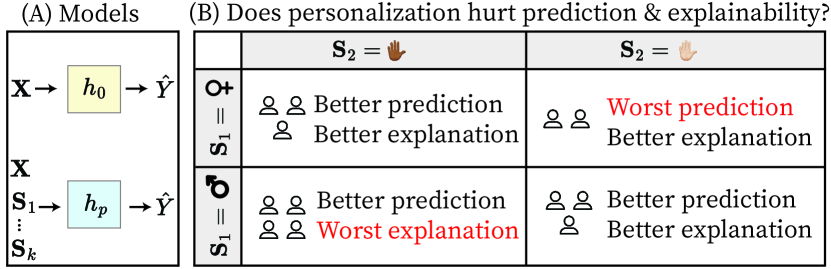
Figure 1: Impact of personalization on fairness in prediction and explainability. (A) Comparison between a generic ML model ($h_{0}$), which uses only input features ($\mathbf{X}$), and a personalized model ($h_{p}$), which incorporates additional personal attributes ($S_{1},\dots,S_{k}$). (B) Group-specific effects on prediction and explanation under personalization. While some groups benefit from improved prediction and explanation, others experience trade-offs, including worsened prediction accuracy or explainability.

Contributions.

This work revisits, unifies, and generalizes previous methodologies to provide a comprehensive understanding of the impact of personalization in ML. More specifically:

• We propose a unifying framework to evaluate personalization in both classification and regression settings.

• Besides prediction accuracy, we provide a novel analysis on how personalization affect the model’s explanation, a perspective absent from the current literature.

• We provide new insights in comparing classification and regression scenarios, demonstrating that regression models can potentially utilize more group attributes than classification models.

• We discover improvements in prediction accuracy from personalization do not necessarily correlate with enhanced explainability. This underscores the importance of evaluating both criteria in models where accuracy and interpretability are paramount.

• We provide guidance to practitioners on how to apply and validate the framework through a real-world dataset example.

		Classification	Regression
	Loss	$C(h)=\Pr(h(\tilde{\mathbf{X}})\neq Y\mid S=s)$	$C(h)=\mathbb{E}\left[\|h(\tilde{\mathbf{X}})-Y\|^{2}\mid S=s\right]$
Predict	Evaluation metric	$C(h)=-\text{AUC}(h,\mathbf{X},Y\mid S=s)$	$C(h)=-R^{2}(h,\mathbf{X},Y\mid S=s)$
	Sufficiency	$C(h)=\Pr(h(\tilde{\mathbf{X}})\neq h(\tilde{\mathbf{X}_{J}})\mid S=s)$	$C(h)=\mathbb{E}\left[\|h(\tilde{\mathbf{X}})-h(\tilde{\mathbf{X}_{J})}\|^{2}\mid S=s\right]$
Explain	Incomprehensiveness	$C(h)=-\Pr\left(h(\tilde{\mathbf{X}})\neq h(\tilde{\mathbf{X}}_{\backslash J})\mid S=s\right)$	$C(h)=-\mathbb{E}\left[\|h(\tilde{\mathbf{X}})-h(\tilde{\mathbf{X}}_{\backslash J})\|^{2}\mid S=s\right]$

Table 1: Personalization benefits group $s$ if the cost of the personalized model is lower than the cost of the generic model for this group. This table shows examples of costs (see Definition 3.1) on data $(\tilde{\mathbf{X}},Y)$ where $\tilde{\mathbf{X}}=\mathbf{X}$ for a generic model $h_{0}$ and $\tilde{\mathbf{X}}=(\mathbf{X},S)$ for a personalized model $h_{p}$. Existing frameworks analyze how personalization impacts predictions in classification settings (in blue). By contrast, our framework applies to all cases provided in this table. We denote by $\mathbf{X}_{\backslash J}$ the input when removing the most important features, and by $\mathbf{X}_{J}$ its complement.

2 Related Works

Personalization. Our research is part of a body of work that investigates how the use of personalized features in machine learning models influences group fairness outcomes (Suriyakumar et al., 2023). Monteiro Paes et al. (2022) defined a metric to measure the smallest gain in accuracy that any group can expect to receive from a personalized model. The authors demonstrate how this metric can be employed to compare personalized and generic models, identifying instances where personalized models produce unjustifiably inaccurate predictions for subgroups that have shared their personal data. However, this literature has focused on the classification framework and has not been generalized to regression tasks. Furthermore, this work has been solely concerned with evaluating how model accuracy is affected, and has not explored how personalizing a model affects the quality of its explanations.

Personalization on Explainability. The field of the effects of personalization on explainable machine learning is largely unexplored. Previous work has investigated gaps in fidelity across subgroups and found that the quality and reliability of explanations may vary across different subgroups (Balagopalan et al., 2022). The work of Balagopalan et al. (2022) trains a human-interpretable model to imitate the behavior of a blackbox model, and characterizes fidelity as how well it matches the blackbox model predictions. To achieve fairness parity, this paper explores using only features with zero mutual information with respect to a protected attribute. However, it left feature importance explanations out of its scope. Additionally, this work neither considers regression tasks nor looks at how personalization affects differences in explanation quality across subgroups.

Fairness. In the field of machine learning, the concept of fairness aims to mitigate biased outcomes affecting individuals or groups (Mehrabi et al., 2022). Past works have defined individual fairness, which requires similar classification for similar individuals with respect to a particular task (Dwork et al., 2011), or group fairness (Dwork & Ilvento, 2019; Hardt et al., 2016), which seeks similar performance across different groups. Within machine learning fairness literature, the majority of methods, metrics, and analyses are predominantly intended for classification tasks, where labels take values from a finite set of values (Pessach & Shmueli, 2022). Among fair regression literature, multiple authors focus on designing fair learning methods rather than developing metrics for measuring fairness in existing models (Berk et al., 2017; Fukuchi et al., 2013; Pérez-Suay et al., 2017; Calders et al., 2013). Complimentary contributions focus on defining fairness criteria and establishing methods to evaluate fairness for regression tasks (Gursoy & Kakadiaris, 2022; Agarwal et al., 2019).

We extend related works tackling explainability in Appendix A.

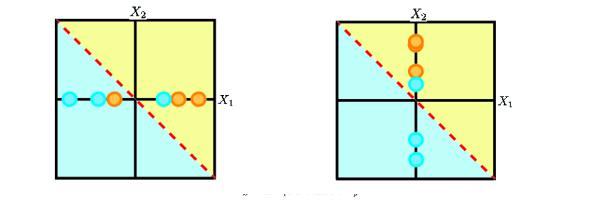
Figure 2: Personalized models should not be dismissed just because they do not provide a clear BoP gain in terms of prediction accuracy: explainability could be improved (see Theorem 4.1). This figure shows the differences between a generic ($h_{0}$) and a personalized ($h_{p}$) model in terms of prediction accuracy and explanation quality –the latter measured by sufficiency and comprehensiveness, defined in Table 1. The generic model $h_{0}$ uses both $X_{1}$ and $X_{2}$ for predictions based on the decision boundary $X_{1}+X_{2}>0$, while $h_{p}$, with access to the group attribute $S=X_{1}+X_{2}$, relies entirely on $S>0$ for predictions (middle column). In the sufficiency evaluation (left column), where only the most important feature is kept, $h_{p}$ achieves perfect prediction since it relies solely on $S$, reaching maximum sufficiency. In contrast, $h_{0}$, using $X_{1}$, has a lower sufficiency score. This demonstrates that personalization enhances explainability, even though prediction accuracy remains the same. In the comprehensiveness evaluation (right column), where the most important feature is removed, $h_{p}$ defaults to random guessing when only $X=(X_{1},X_{2})$ is available, as it never learned to use $X_{1}$ or $X_{2}$. This results in $h_{p}$ achieving the minimum comprehensiveness value, indicating the best explanation performance. Conversely, $h_{0}$ shows a higher comprehensiveness score. Again, personalization improves explainability according to this measure, without affecting prediction accuracy.

3 Background: Benefit of Personalization

This section provides the necessary background to introduce and contextualize our framework, designed to evaluate the impact of personalized machine learning models.

Within a supervised learning setting, a personalized model $h_{p}:\mathcal{X}\times\mathcal{S}\rightarrow\mathcal{Y}$ aims to predict an outcome variable $Y\in\mathcal{Y}$ using both an input feature vector $X\in\mathcal{X}$ and a vector of group attributes $S\in\mathcal{S}$. In contrast, a generic model $h_{0}:\mathcal{X}\rightarrow\mathcal{Y}$ does not use (sensitive) group attributes. We assume that the models $h_{0},h_{p}$ are trained on a training dataset that is independent of the auditing dataset $\mathcal{D}$. We consider that a fixed data distribution $P_{\mathbf{X},\mathbf{S},Y}$ is given, and that $h_{0}$ and $h_{p}$ models minimize the loss over the training dataset $\mathcal{D}_{train}$.

Definition 3.1 (Model cost).

The cost of a model $h$ with respect to a cost function $\mathrm{cost}:\mathcal{Y}\times\mathcal{Y}\rightarrow\mathbb{R}$ is defined as:

$$\begin{split}C(h)&\triangleq\mathbb{E}[\mathrm{cost}(h,\tilde{\mathbf{X}},Y)]~\text{(population)},\quad\\ C(h,\mathbf{s})&\triangleq\mathbb{E}[\mathrm{cost}(h,\tilde{\mathbf{X}},Y)\mid\mathbf{S}=\mathbf{s}]~\text{(for group $s$)},\end{split}$$ (1)

where $\tilde{\mathbf{X}}=\mathbf{X}$ for a generic models $h_{0}$, and $\tilde{\mathbf{X}}=(\mathbf{X},\mathbf{S})$ for a personalized model $h_{p}$. See Appendix B for the estimates of the quantities defined above.

For example, we may want to evaluate the accuracy of the prediction of a given supervised learning model. In this case, the cost function can be the loss function used to train the model (e.g. mean squared error loss for regression, 0-1 loss for binary classification), or any auxiliary evaluation function (such as area-under-the-curve for binary classification). Alternatively, we may want to evaluate the quality of the explanations given by an explanation method. In this case, the cost function can be one of the measures of quality of explanations, such as sufficiency which is a form of deletion of features (see Nauta et al. (2023) for a review). In this paper we utilize incomprehensivenss and sufficiency, which measure how much model prediction changes when removing or keeping the features deemed most important in the explanation. However, while this paper focuses on prediction accuracy and explanation quality, we emphasize that the definition above –as well as our proposed framework– can be applied to any cost function, i.e., to any quantitative evaluation of the properties of a model.

In what follows, we assume that lower cost means better performance. We can thus quantify the impact of a personalized model in terms of the benefit of personalization, defined next.

Definition 3.2 (Benefit of Personalization (BoP)).

The gain from personalizing a model can be measured by comparing the costs of the generic and personalized models:

$$\begin{split}\operatorname{BoP}(h_{0},h_{p})&\triangleq C(h_{0})-C(h_{p})~\text{(population)},\\ \quad\operatorname{BoP}(h_{0},h_{p},\mathbf{s})&\triangleq C(h_{0},\mathbf{s})-C(h_{p},\mathbf{s})~\text{(group $s$)}.\end{split}$$ (2)

By convention, $\operatorname{BoP}>0$ when the personalized model $h_{p}$ performs better than the generic model $h_{0}$. The estimates are: $\operatorname{\hat{BoP}}(h_{0},h_{p})=\hat{C}(h_{0})-\hat{C}(h_{p})$ and $\operatorname{\hat{BoP}}(h_{0},h_{p},s)=\hat{C}(h_{0},s)-\hat{C}(h_{p},s)$. When using $\operatorname{BoP}$ to evaluate improvement in predictive accuracy and explanation quality, it is referred to as BoP-P and BoP-X, respectively.

In Appendix C, we provide examples showing how these abstract definitions can be used to measure BoP for both predictions and explanations, each across both classification and regression tasks.

It is crucial to consider if personalization benefits each subgroup equally, and more so to investigate whether personalization actively harms particular subgroups (Monteiro Paes et al., 2022). The following concept is useful to identify the latter scenario:

Definition 3.3 (Minimal Group BoP).

The Minimal Group Benefit of Personalization (BoP) is defined as the minimum BoP value across all subgroups $s\in S$:

$$\gamma\left(h_{0},h_{p}\right)\triangleq\min_{\mathbf{s}\in\mathcal{S}}(\operatorname{BoP}(h_{0},h_{p},\mathbf{s})).$$ (3)

The estimate is $\hat{\gamma}\left(h_{0},h_{p}\right)\triangleq\min_{\mathbf{s}\in\mathcal{S}}(\operatorname{\hat{BoP}}(h_{0},h_{p},s))$.

It captures the worst-case subgroup performance improvement, or the worst degradation, resulting from personalization. A positive Minimal Group BoP indicates that all subgroups receive better performance with respect to the cost function. Contrary to this, a negative value reflects that at least one group is disadvantaged by the use of personal attributes. When the Minimal Group BoP is small or negative, the practitioner might want to reconsider the use of personalized attributes in terms of fairness with respect to all subgroups.

4 Impact of Personalization on Prediction And Explainability

In this section, we highlight different scenarios that can arise when personalizing machine learning models. First, we provide a comparison of how personalization impacts prediction and explainability.

Absence of Benefit in Prediction Does not Imply Absence of Benefit in Explainability. The following theorem emphasizes the necessity of assessing the BoP in terms of both predictive accuracy (BoP-P) and explainability (BoP-X).

Theorem 4.1.

There exists a data distribution $P_{\mathbf{X},\mathbf{S},Y}$ such that the Bayes optimal classifiers $h_{0}$ and $h_{p}$ satisfy $\text{BoP-P}(h_{0},h_{p})=0$ and $\text{BoP-X}(h_{0},h_{p})>0$

Therefore, a personalized model may not have superior predictive performance yet still improve explainability. Or, in other words, evaluating personalized models solely on predictive accuracy risks can overlook substantial gains in interpretability. Figure 2 illustrates this with a simple example where personalization doesn’t affect prediction accuracy, but it does improve explainability.

Absence of Benefit in Explainability Can Imply Absence of Benefit in Prediction. For a simple additive model, we can show that $\text{BoP-X}=0$ does imply $\text{BoP-P}=0$. Note that, by $\text{BoP-X}=0$, we mean both sufficiency and comprehensiveness do not improve with personalization. Proving this for a general class of model remains an open question.

Theorem 4.2.

Assume that $h_{0}$ and $h_{p}$ are Bayes optimal classifiers and $P_{\mathbf{X},\mathbf{S},Y}$ follows an additive model, i.e.,

$$Y=\alpha_{1}X_{1}+\cdots+\alpha_{t}X_{t}+\alpha_{t+1}S_{1}+\cdots+\alpha_{t+k}S_{k}+\epsilon,$$ (4)

where $X_{1},\cdots,X_{t}$ and $S_{1},\cdots,S_{k}$ are independent, and $\epsilon$ is an independent random noise. Then, if $\text{BoP-X}(h_{0},h_{p})=0$, then $\text{BoP-P}(h_{0},h_{p})=0$.

This theorem demonstrates that under an additive model, if there is no benefit in explanation quality, then there is also no benefit in prediction accuracy. It establishes a direct link between explanation and prediction and underscores its importance in the simplified linear setting. Additionally, this means that if $\text{BoP-P}(h_{0},h_{p})\neq 0$, then $\text{BoP-X}(h_{0},h_{p})\neq 0$.

5 Testing the Impact of Personalization

Calculating the BoP requires exact knowledge of the data distribution, a condition rarely met in practice. Within the ubiquitous finite sample regime, it is critical to understand the reliability of the empirical BoP: if we compute a positive empirical BoP on the audit dataset, does this mean that the true, unknown BoP is also positive?

Drawing inspiration from (Monteiro Paes et al., 2022), we consider the most natural hypothesis testing framework to assess whether a personalized model yields a substantial performance improvement across all groups. Subsequently, we derive a novel information-theoretic bound on the reliability of this procedure.

Proofs for theorems, lemmas and corollaries are in Appendices D.1, D.3, D.5, D.8, E and F.

Hypothesis Test Given an auditing dataset $\mathcal{D}$, we verify whether using a personalized model $h_{p}$ yields an $\epsilon>0$ gain in expected performances compared to using a generic model $h_{0}$. The improvement $\epsilon$ is in cost function units, and corresponds to the reduction in cost for the group for which moving from $h_{0}$ to $h_{p}$ is least advantageous –i.e., $\epsilon$ represents the improvement for the group that benefits the least from the personalized model. The null and the alternative hypotheses of the test write:

$$H_{0}:\gamma(h_{0},h_{p};\mathcal{D})\leq 0\Leftrightarrow h_{p}$$ Personalized does not bring

any gain for at least one group,

$$H_{1}:\gamma(h_{0},h_{p};\mathcal{D})\geq\epsilon\Leftrightarrow h_{p} \epsilon$$ Personalized yields at least

improvement for all groups.

To perform the hypothesis test, we follow (Monteiro Paes et al., 2022) and use the threshold test on the estimate of the BoP $\hat{\gamma}$:

$$\hat{\gamma}\geq\epsilon\Rightarrow H_{0}$$ Reject : Conclude that personalization yields

at least $$\epsilon$$ improvement for all groups.

Reliability of the Test We are interested in characterizing the reliability of the hypothesis test: in other words, can we trust the value of the empirical $\hat{\gamma}$ ? We characterize the reliability of the test in terms of its probability of error, $P_{e}$, defined as:

$$P_{e}= \ \text{Pr}(\text{Type I error})+\text{Pr}(\text{Type II error})$$

$$= \ \text{Pr}(\text{Rejecting $H_{0}$}|\text{$H_{0}$ is true})+$$

$$\ \text{Pr}(\text{Failing to reject $H_{0}$}|\text{$H_{1}$ is true}).$$

If this probability exceeds 50%, the test is no more reliable than the flip of a fair coin, making it too untrustworthy to support any meaningful verification. Therefore, it would be practical to compute a lower bound on the worst case scenario for this probability of error, so that if this lower bound exceeds 50%, we would not trust the test. We precisely derive the bound for a general cost function, such that it applies for any prediction (regression and classification) and any explainability quality measures.

In particular, a minimax bound is used to establish a lower bound on $P_{e}$. This involves considering the worst-case data distributions that maximizes $P_{e}$ and the best possible decision function $\Psi$ that minimizes it. Assuming that the value of $\epsilon$ is fixed, we provide the following result:

Theorem 5.1 (Lower bound for BoP).

The lower bound writes:

$$\min_{\Psi}\max_{\begin{subarray}{c}P_{0}\in H_{0}\\ P_{1}\in H_{1}\end{subarray}}P_{e}\geq 1-\frac{1}{2\sqrt{d}}\left[\frac{1}{d}\sum_{j=1}^{d}\mathbb{E}_{p^{\epsilon}}\Bigg{[}\frac{p^{\epsilon}(B)}{p(B)}\Bigg{]}^{m_{j}}-1\right]^{\frac{1}{2}}$$ (5)

where $P_{\mathbf{X},\mathbf{S},Y}$ is a distribution of data, for which the generic model $h_{0}$ performs better, i.e., the true $\gamma$ is such that $\gamma(h_{0},h_{p},\mathcal{D})<0$, and $Q_{\mathbf{X},\mathbf{S},Y}$ is a distribution of data points for which the personalized model performs better, i.e., the true $\gamma$ is such that $\gamma(h_{0},h_{p},\mathcal{D})\geq\epsilon$. Dataset $\mathcal{D}$ is drawn from an unknown distribution and has $d$ groups where $d=2^{k}$, with each group $j$ has $m_{j}$ samples. The probabilities $p$ and $p_{\epsilon}$ refer to distributions of the individual BoP, i.e., $B=C(h_{0},X,Y)-C(h_{p},X,Y)$, where every individual follows $p(B)$, except for individuals in one group which follow $p^{\epsilon}(B)$.

This lower bound reflects the worst-case performance of any hypothesis test, by exhibiting a pair of distributions—one under $H_{0}$ and the other under $H_{1}$—for which the probability error $P_{e}$ test will be greater than or equal to the lower bound. Hence, this theorem offers a practical method to assess whether we should trust the value of the empirical benefit (or risk) of a personalized model. If the probability distribution of individual BoP is known, practitioners can directly compute the lower bound specific to their case. If unknown, the distribution can be estimated beforehand. The method proceeds as follows: 1) fit the generic model $h_{0}$ and the personalized model $h_{p}$, 2) plot the histograms of the individual BoP and identify its probability distribution (Gaussian, Laplace, etc.), and 3) apply Theorem 5.1 to evaluate whether the observed BoP is sufficient. For completeness, we provide in the corollary below the value of the lower bound for any distribution in the exponential family.

Corollary 5.2 (Lower Bound Exponential Family Distributions).

Consider $p$ a distribution in the exponential family with natural parameter $\theta$ and $M_{p}$ the moment generating function of its sufficient statistic. The lower bound for the probability of the error in the hypothesis test is:

$$\min_{\Psi}\max_{\begin{subarray}{c}P_{0}\in H_{0}\\ P_{1}\in H_{1}\end{subarray}}P_{e}$$

$$\geq 1-\frac{1}{2\sqrt{d}}\Bigg{[}\frac{1}{d}\sum_{j=1}^{d}\left(\frac{M_{p}(2\Delta\theta)}{M_{p}(\Delta\theta)^{2}}\right)^{m_{j}}-1\Bigg{]}^{\frac{1}{2}}$$

$$=1-\frac{1}{2\sqrt{d}}\Bigg{[}\frac{1}{d}\sum_{j=1}^{d}\left(1+4\epsilon^{2}\right)^{m_{j}}-1\Bigg{]}^{\frac{1}{2}}~\text{(Categorical)}$$

$$=1-\frac{1}{2\sqrt{d}}\Bigg{[}\frac{1}{d}\sum_{j=1}^{d}\exp\left(\frac{{m_{j}}\epsilon^{2}}{\sigma_{j}^{2}}\right)-1\Bigg{]}^{\frac{1}{2}}~\text{(Gaussian)}$$

In the case of categorical distributions, this result generalizes the result in (Monteiro Paes et al., 2022), by providing a finer bound where the groups are also not constrained to have the same number of samples. Appendix D.7 also provides the formula for any probability distribution in the symmetric generalized Gaussian family. The Laplace distribution lower bound is found from this and provided below.

Corollary 5.3 (Lower bound Laplace Distribution).

The lower bound for the probability of the error in the hypothesis test is:

$$\min_{\Psi}\max_{\begin{subarray}{c}P_{0}\in H_{0}\\ P_{1}\in H_{1}\end{subarray}}P_{e}$$

$$\geq 1-\frac{1}{2\sqrt{d}}\left[\frac{1}{d}\sum_{j=1}^{d}\exp\left(-\frac{m_{j}\epsilon}{b_{j}}\right)-1\right]^{\frac{1}{2}}~\text{(Laplace)}.$$

These results characterize how the probability of error relates to the number $k$ of group attributes, which defines the number $d=2^{k}$ of groups, and to the number of samples per group. Fewer samples per group lead to a higher chance of error in hypothesis testing, thus yielding a fundamental limit on the maximum number of group attributes a personalized model can handle to ensure every group benefits, without relying on additional data distribution assumptions. These ideas are made concrete by the following results.

Maximum Number of Personal Attributes Given the lower bound obtained in Corollary 5.2 and 5.3, we compute the maximum number of attributes $k$ for which testing the benefit of personalization makes sense. Here, we assume that each group $j$ has the same number of samples $m_{j}=m=\left[\frac{N}{d}\right]$.

Corollary 5.4 (Maximum number of attributes).

If we wish to maintain a probability of error such that $\min\max P_{e}\leq 1/2$, then the number of attributes $k$ should be chosen below a value $k_{\max}$ such that:

$$k_{max} =1.4427W\left(N\log(4\epsilon^{2}+1)\right)~\text{(Categorical BoP)}$$

$$=1.4427W\left(\frac{\epsilon^{2}N}{\sigma^{2}}\right)~\text{(Gaussian BoP, variance $\sigma^{2}$)}$$

$$=1.4427W\left(\frac{-\epsilon N}{b}\right)~\text{(Laplace BoP, scale $b$)},$$

where $W$ is the Lambert W function.

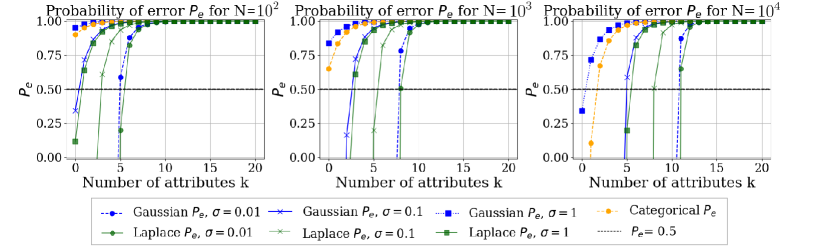
Figure 3: Lower bound of the probability of error $P_{e}$ versus number of attributes $k$, defining the number of groups $d=2^{k}$ for $\epsilon=0.01$. For three different number of samples $N$, we consider a categorical BoP (orange), Gaussian BoPs with different variance $\sigma^{2}$ (blue), and Laplace BoPs with several scale parameters $b=\frac{\sigma}{\sqrt{2}}$. We see that for small $\sigma$ values in the Gaussian case, the number of attributes $k$ that can be used before surpassing $P_{e}\geq 1/2$ is higher than for the categorical case. The Laplace case surpasses the categorical in all cases, and the Gaussian in most. For this example, we utilize the $P_{e}$ functions assuming each group has $m=\lfloor\frac{N}{d}\rfloor$ samples.

From this corollary, we first see that there is an absolute limit in the number of personal attributes that can be input to any model where each data point represents one person: the number $k_{\text{max}}$ for $N$ equal to its maximum value, i.e., the number of people on the planet, is equal to 18, 22, and 26 binary attributes for Categorical, Gaussian, and Laplace BoP distributions, respectively.

Next, given a single dataset, the maximum number of personal attributes allowed to test for the benefit of personalization depends on the machine learning model: classification versus regression.

Classification Versus Regression Figure 3 plots the relation between $k$ and the lower bound of $P_{e}$ for common sample sizes in medical applications, contrasting classification versus regression cases. The BoP is assumed to be Gaussian of variance $\sigma^{2}$ for the regression. We clearly observe the consequences of the extra dependency on $\sigma$. Small values of $\sigma$ allow for a higher number of personal attributes $k_{\text{max}}$ in regression compared to the classification case. This means that we can rely on the value of the empirical BoP to test whether there is indeed a benefit of a personalized regression model, even when a high number of personal attributes are used. This tells a much more subtle story than for the classification case, because the maximum number of attributes allowed depends on the distribution of the BoP across participants.

Prediction versus Explainability

Within the setting of classification, the maximum number of personal attributes allowed does not differ in prediction versus explainability: both utilize an individual cost function that can be described by a Bernoulli random variable. Within the setting of regression, the maximum number of attributes can differ between prediction and explainability, for both sufficiency and incomprehensiveness. This is because this number depends on the distribution of the individual BoP and the standard deviation of the BoP across participants. Therefore, the number of allowed attributes will differ provided this value is different for each criteria evaluated.

6 Experiments

This section shows how we can apply the framework to determine whether personalization benefits classification and regression tasks, leveraging to that end the validation tools developed in previous Section 5.

Dataset. We apply our framework to the MIMIC-III Clinical Database (Johnson et al., 2016) utilizing two binary group attributes: $\mathrm{Age}\times\mathrm{Race}\in\{\mathrm{\mathrm{18-45}},\mathrm{45+}\}\times\{\mathrm{White(W)},\mathrm{NonWhite(NW)}\}$. For the regression task, the goal is to predict the patient length of stay. For the binary classification task, the goal is to predict if length of stay $>3$ days. We consider a 70/30 split for training and test sets on both classification and regression, fitting two neural network models in each setting: one with a one-hot encoding of the group attributes ($h_{p}$), and the other without group attributes ($h_{0}$). Lastly, regression prediction values are normalized to have mean 0 and standard deviation 1.

Explainability Method. We generate model explanations with the Captum Integrated gradient explainer method (Sundararajan et al., 2017). This method calculates the gradient of the output with respect to the input for each subject, and scales the result to get an importance value for each input feature. To evaluate BoP-X using sufficiency and incomprehensivess, we select an value $r$ such that $50\%$ of features are kept or removed. Plots in Appendix G.1 depict how sufficiency and incomprehensiveness change for different values of $r$, as well as show the individual BoP distributions.

Classification Results
Group	$n$	Prediction	Incomp.	Sufficiency
White, 45+	8443	0.0063	-0.0226	0.0053
White, 18-45	1146	0.0044	0.0489	0.0244
NonWhite, 45+	3052	-0.0026	-0.0023	0.0029
NonWhite, 18-45	696	-0.0216	0.0560	0.0072
All Pop.	13337	0.0026	-0.0077	0.0065
Minimal BoP	13337	-0.0216	-0.0226	0.0029
Regression Results
Group	$n$	Prediction	Incomp.	Sufficiency
White, 45+	8379	0.0021	-0.0906	0.1914
White, 18-45	1197	0.0023	0.1219	0.2223
NonWhite, 45+	3044	0.0108	-0.0501	0.3494
NonWhite, 18-45	717	0.0212	0.0441	0.3293
All Pop.	13337	0.0051	-0.0550	0.2376
Minimal BoP	13337	0.0021	-0.0906	0.1914

Table 2: Experimental results on the test set of the MIMIC-III dataset for both classification and regression. All columns show the value of $\hat{C}(h_{0})-\hat{C}(h_{p})$ evaluated for the corresponding metric. Incomprehensiveness is abbreviated as incomp. and population as pop. Values that are worsened by $h_{p}$ are colored red.

Experimental Results. Table 2 shows full results of the Population, Groupwise, and Minimal Group BoP on the test set. The 0-1 and square loss cost functions are used for classification and regression. From these tables in the regression task, we see subgroups for whom BoP-P is positive, while BoP-X is negative. In the classification task, personalization improves prediction and sufficiency, whereas it worsens incomprehensiveness for some subgroups.

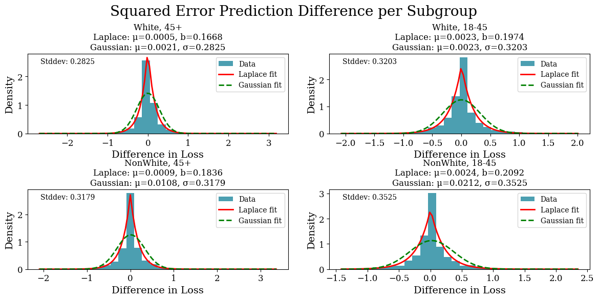
Figure 6: Individual prediction cost for all groups using the square error loss function.

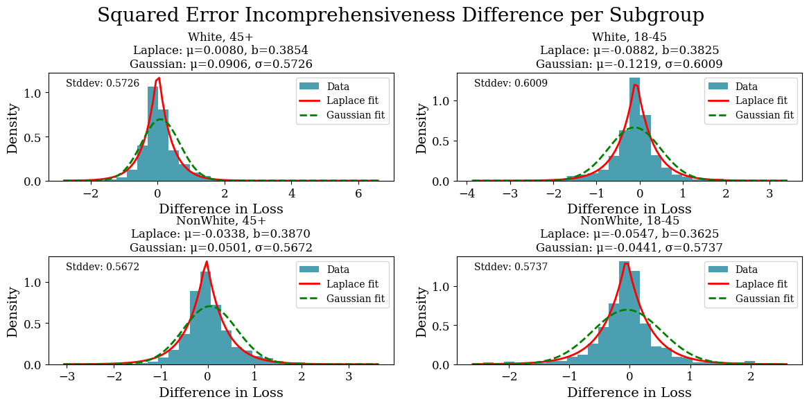
Figure 7: Individual incomprehensiveness cost for all groups using the square error loss function.

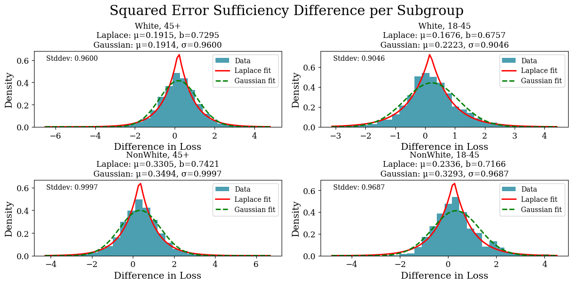
Figure 8: Individual sufficiency cost for all groups using the square error loss function.

Statistical Validation. To better understand the reliability of our empirical results, we apply the procedure described in the previous section. First, we plot the histograms of the individual BoP for the regression task, as shown in Figures 6, 7, and 8 in Appendix G.1. For the classification task, these distributions will all be categorical. Next, we estimate the probability distribution family that has generated these empirical distributions. In the sufficiency case, this is best fit by a family of Gaussian distributions with different variances. In the prediction and incomprehensiveness cases, these are best fit by Laplace distributions with different scale parameters. Lastly, Figure 4 shows the information-theoretic lower bound on probability of error that our validation framework provides (Corollary 5.2, 5.3) for this dataset and these tasks. This lower bound is a function of $\epsilon$, which is the minimum improvement across all groups from the personalized model required to reject the null hypothesis.

In particular, we get that there is no fundamental limit against trusting our results for $\hat{\gamma}_{BoP}>0.009$ for all metrics in the classification task. In the regression scenario, we find the thresholds $(i)$ $\hat{\gamma}_{BoP-P}>6.53\cdot 10^{-5}$ for prediction accuracy, $(ii)$ $\hat{\gamma}_{BoP-X}>1.29\cdot 10^{-4}$ for incomprehensiveness, and $(iii)$ $\hat{\gamma}_{BoP-X}>0.017$ for sufficiency. These values can be seen on Figure 4 as the locations where each of the lines cross ${P_{e}=0.5}$, which corresponds to the smallest $\epsilon$ needed to ensure the lower bound on the probability of error does not exceed $50\%$. These plots are made using the unique $n,\sigma$ and $b$ values of each individual BoP distribution for this experiment. Utilizing these plots, practitioners can verify if the hypothesis test remains reliable under $\epsilon$. Given a reliable test, they then can either reject, or fail to reject the null hypothesis using their empirical minimal BoP values.

BoP-P Analysis. In the case of prediction accuracy, we observe that the personalized model $h_{p}$ assigns less accurate predictions to specific subgroups in the classification task –even decreasing the overall accuracy for the entire population. Hence, the minimal BoP-P is negative and there is no evidence in favor of a benefit. For regression, all subgroups are benefited by personalization and we can reject the null hypothesis if $\epsilon$ has been set at below $0.0021$, the empirical minimal BoP-P.

BoP-X Analysis. In the case of explainability, sufficiency is improved by personalization for all subgroups across regression and classification. We can reject $H_{0}$ if $\epsilon$ has been set below $0.1914$ and $0.0029$, respectively. However, incomprehensiveness improves for some subgroups and worsens for others, resulting in a negative minimal BoP-X for both.

BoP-P vs. BoP-X. For regression, we see a benefit from personalization in terms of both prediction and sufficiency. For classification, we see a benefit for sufficiency alone. This illustrates two cases: one where prediction is not improved, but an aspect of explainability is; and another where prediction is improved, but an aspect of explainability is not. A negative BoP in the other values impedes us to draw conclusions about any potential benefit from personalizing.

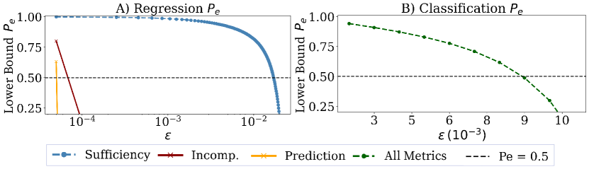
Figure 4: Leveraging the validation framework, we plot how the $P_{e}$ changes for different $\epsilon$ values for a set $N$ and $k=2$ using Corollary 5.2 and 5.3. We utilize the Laplace and Gaussian form in A, and the Categorical in B.

7 Concluding Remarks

This work introduces a novel BoP framework that accommodates model accuracy and explainability, both of which are paramount to building trust and transparency in sensitive settings. Additionally, the framework also extends the BoP analysis to regression tasks, enabling its application to new non-discretized scenarios. Through our theoretical analysis, we identified conditions for regression and classification where testing and estimation methods lack sufficient reliability to guarantee improvements across subgroups. Our findings also reveal that regression tasks have the potential to benefit from more personalized attributes than classification tasks, and that improved accuracy from personalization does not necessarily translate to enhanced explainability. Finally, and as exemplified by our evaluation, our framework and accompanying tests facilitate nuanced decisions regarding the use of protected attributes. Overall, this paper broadens the scope and applicability of BoP analysis and in doing so contributes to the selection of more fair and interpretable models.

Impact Statement

This paper presents work whose goal is to advance the field of Machine Learning. There are many potential societal consequences of our work. Our work will give machine learning practioners a framework to assess if including personal attributes in their models (i.e. sex, age, race), provides a benefit in model accuracy and the quality of a model explanations.

Appendix A Extended Related Works: Explainability

Explainability Typical approaches to model explanation involve measuring how much each input feature contributes to the model’s output, highlighting important inputs to promote user trust. This process often involves using gradients or hidden feature maps to estimate the importance of inputs (Simonyan et al., 2014; Smilkov et al., 2017; Sundararajan et al., 2017; Yuan et al., 2022). For instance, gradient-based methods use backpropagation to compute the gradient of the output with respect to inputs, with higher gradients indicating greater importance (Sundararajan et al., 2017; Yuan et al., 2022). The quality of these explanations is often evaluated using the principle of faithfulness (Lyu et al., 2024; Dasgupta et al., 2022; Jacovi & Goldberg, 2020), which measures how accurately an explanation represents the reasoning of the underlying model. Two key aspects of faithfulness are sufficiency and comprehenesiveness (DeYoung et al., 2020; Yin et al., 2022); the former assesses whether the inputs deemed important are adequate for the model’s prediction, and the latter examines if these features capture the essence of the model’s decision-making process.

Appendix B Empirical Definitions

Below, we provide estimates of the population and group cost quantities.

B.1 Cost

Definition B.1 (Population Cost).

The empirical individual cost, of a model $h$ for subject $i$ with respect to a cost function, $\mathrm{cost}:\mathcal{Y}\times\mathcal{Y}\rightarrow\mathbb{R}$ is defined as:

$$\hat{C_{s}}(h,\mathbf{s})\triangleq\left\{\begin{array}[]{lll}\frac{1}{N}\sum_{i=1}^{N}\mathrm{cost}\left(h\left(\mathbf{x}_{i}\right),y_{i}\right)&\text{ if }&h:\mathcal{X}\rightarrow\mathcal{Y}\quad\text{ (generic model) }\\ \frac{1}{N}\sum_{i=1}^{N}\mathrm{cost}\left(h\left(\mathbf{x}_{i},\mathbf{s}_{i}\right),y_{i}\right)&\text{ if }&h:\mathcal{X}\times\mathcal{S}\rightarrow\mathcal{Y}\quad\text{ (personalized model) }\end{array}\right.$$ (6)

where $N$ refers to the total number of samples$\mathbf{s}$.

Definition B.2 (Group Cost).

The empirical group cost, $\hat{C_{s}}(h,\mathbf{s})$, is defined as:

$$\hat{C_{s}}(h,\mathbf{s})\triangleq\left\{\begin{array}[]{lll}\frac{1}{n_{\mathbf{s}}}\sum_{i:\mathbf{s}_{i}=\mathbf{s}}\mathrm{cost}\left(h\left(\mathbf{x}_{i}\right),y_{i}\right)&\text{ if }&h:\mathcal{X}\rightarrow\mathcal{Y}\quad\text{ (generic model) }\\ \frac{1}{n_{\mathbf{s}}}\sum_{i:\mathbf{s}_{i}=\mathbf{s}}\mathrm{cost}\left(h\left(\mathbf{x}_{i},\mathbf{s}_{i}\right),y_{i}\right)&\text{ if }&h:\mathcal{X}\times\mathcal{S}\rightarrow\mathcal{Y}\quad\text{ (personalized model) }\end{array}\right.$$ (7)

where $n_{\mathrm{s}}$ refers to the number of samples in group $\mathbf{s}$.

Appendix C BoP

In the following table, we how these abstract definitions can be used to measure BoP for both predictions and explanations, each across both classification and regression tasks.

$$\scriptsize\begin{array}[]{|c|c|}\hline\cr\textbf{Evaluation Type}&\textbf{Benefit of personalization for group $s$}\\ \hline\cr\text{Predict (Classification, 0-1 loss)}&\Pr(h_{0}(\mathbf{X})\neq Y\mid S=s)-\Pr(h_{p}(\mathbf{X},s)\neq Y\mid S=s)\\ \hline\cr\text{Predict (Regression, MSE)}&\mathbb{E}\left[\|h_{0}(\mathbf{X})-Y\|^{2}\mid S=s\right]-\mathbb{E}\left[\|h_{p}(\mathbf{X},s)-Y\|^{2}\mid S=s\right]\\ \hline\cr\text{Explain (Sufficiency, classification, 0-1 loss)}&\Pr(h_{0}(\mathbf{X})\neq h_{0}(\mathbf{X}_{J})\mid S=s)-\Pr(h_{p}(\mathbf{X},s)\neq h_{p}(\mathbf{X}_{J},s_{J})\mid S=s)\\ \hline\cr\text{Explain (Sufficiency, regression, MSE)}&\mathbb{E}\left[\|h_{0}(\mathbf{X})-h_{0}(\mathbf{X}_{J})\|^{2}\mid S=s\right]-\mathbb{E}\left[\|h_{p}(\mathbf{X},s)-h_{p}(\mathbf{X}_{J},s_{J})\|^{2}\mid S=s\right]\\ \hline\cr\text{Explain (Incomprehensiveness, classification, 0-1 loss)}&\operatorname{Pr}\left(h_{p}(\mathbf{X},s)\neq h_{p}(\mathbf{X}_{\backslash J},s_{\backslash J})\mid S=s\right)-\left.\operatorname{Pr}\left(h_{0}(\mathbf{X})\neq h_{0}(\mathbf{X}_{\backslash J})\mid S=s\right)\right)\\ \hline\cr\text{Explain (Incomprehensiveness, regression, MSE)}&\mathbb{E}\left[\|h_{p}(\mathbf{X},s)-h_{p}(\mathbf{X}_{\backslash J},s_{\backslash J})\|^{2}\mid S=s\right]-\left.\mathbb{E}\left[\|h_{0}(\mathbf{X})-h_{0}(\mathbf{X}_{\backslash J})\|^{2}\mid S=s\right]\right)\\ \hline\cr\end{array}$$

Appendix D Proof of Theorems on Lower Bounds for the Probability of error

As in (Monteiro Paes et al., 2022), we will prove every theorem for the flipped hypothesis test defined as:

$$H_{0}: \gamma(h_{0},h_{p};\mathcal{D}) \leq\epsilon\quad\Leftrightarrow\quad\text{Personalized $h_{p}$ performs worst: yields $\epsilon<0$ disadvantage}$$

$$H_{1}: \gamma(h_{0},h_{p};\mathcal{D}) \geq 0\quad\Leftrightarrow\quad\text{Personalized $h_{p}$ performs at least as good as generic $h_{0}$.}$$

where we emphasize that $\epsilon<0$.

As shown in (Monteiro Paes et al., 2022), proving the bound for the original hypothesis test is equivalent to proving the bound for the flipped hypothesis test, since estimating $\gamma$ is as hard as estimating $-\gamma$. In every section that follows, $H_{0},H_{1}$ refer to the flipped hypothesis test.

Here, we first prove a proposition that is valid for all of the cases that we consider in the next sections.

Proposition D.1.

Consider $P_{\mathbf{X},\mathbf{S},Y}$ is a distribution of data, for which the generic model $h_{0}$ performs better, i.e., the true $\gamma$ is such that $\gamma(h_{0},h_{p},\mathcal{D})<0$, and $Q_{\mathbf{X},\mathbf{S},Y}$ is a distribution of data points for which the personalized model performs better, i.e., the true $\gamma$ is such that $\gamma(h_{0},h_{p},\mathcal{D})>0$. Consider a decision rule $\Psi$ that represents any hypothesis test. We have the following bound on the probability of error $P_{e}$:

$$\min_{\Psi}\max_{\begin{subarray}{c}P_{0}\in H_{0}\\ P_{1}\in H_{1}\end{subarray}}P_{e}\geq 1-TV(P\parallel Q),$$

for any well-chosen $P\in H_{0}$ and any well-chosen $Q\in H_{1}$. Here $TV$ refers to the total variation between probability distributions $P$ and $Q$.

Proof.

Consider $h_{0}$ and $h_{p}$ fixed. Take one decision rule $\Psi$ that represents any hypothesis test. Consider a dataset such that $H_{0}$ is true, i.e., $\mathcal{D}\sim P_{0}$ and a dataset such that $H_{1}$ is true, i.e., $\mathcal{D}\sim P_{1}$.

It might seem weird to use two datasets to compute the same quantity $P_{e}$, i.e., one dataset to compute the first term in $P_{e}$, and one dataset to compute the second term in $P_{e}$. However, this is just a reflection of the fact that the two terms in $P_{e}$ come from two different settings: $H_{0}$ true or $H_{0}$ false, which are disjoint events: in the same way that $H_{0}$ cannot be simultaneously true and false, yet each term in $P_{e}$ consider one or the other case; then we use one or the other dataset.

We have:

$$P_{e} =\text{Pr}(\text{Rejecting $H_{0}$}|\text{$H_{0}$ true})+\text{Pr}(\text{Failing to reject $H_{0}$}|\text{$H_{1}$ true})$$

$$=\text{Pr}(\Psi(h_{0},h_{p},\mathcal{D},\epsilon)=1|\mathcal{D}\sim P_{0})+\text{Pr}(\Psi(h_{0},h_{p},\mathcal{D},\epsilon)=0|\mathcal{D}\sim P_{1})$$

$$=\text{Pr}(\Psi(\mathcal{D})=1|\mathcal{D}\sim P_{0})+\text{Pr}(\Psi(\mathcal{D})=0|\mathcal{D}\sim P_{1})~\text{simplifying notations}$$

$$=1-\text{Pr}(\Psi(\mathcal{D})=0|\mathcal{D}\sim P_{0})+\text{Pr}(\Psi(\mathcal{D})=0|\mathcal{D}\sim P_{1})~\text{complementary event}$$

$$=1-P_{0}(E_{\Psi})+P_{1}(E_{\Psi})~\text{writing $E_{\Psi}$ the event $\Psi(\mathcal{D})=0$}$$

$$=1-(P_{0}(E_{\Psi})-P_{1}(E_{\Psi}))$$

Now, we will bound this quantity:

$$\min_{\Psi}\max_{\begin{subarray}{c}P_{0}\in H_{0}\\ P_{1}\in H_{1}\end{subarray}}P_{e} =\min_{\Psi}\max_{\begin{subarray}{c}P_{0}\in H_{0}\\ P_{1}\in H_{1}\end{subarray}}1-(P_{0}(E_{\Psi})-P_{1}(E_{\Psi}))$$

$$\geq\max_{\begin{subarray}{c}P_{0}\in H_{0}\\ P_{1}\in H_{1}\end{subarray}}\min_{\Psi}\left[1-(P_{0}(E_{\Psi})-P_{1}(E_{\Psi}))\right]~\text{using minmax inequality}$$

$$=\max_{\begin{subarray}{c}P_{0}\in H_{0}\\ P_{1}\in H_{1}\end{subarray}}\left[1-\max_{\Psi}(P_{0}(E_{\Psi})-P_{1}(E_{\Psi}))\right]~\text{to get min over $\Psi$, we want $(P_{0}(E_{\Psi})-P_{1}(E_{\Psi}))$ that is largest.}$$

$$\geq\max_{\begin{subarray}{c}P_{0}\in H_{0}\\ P_{1}\in H_{1}\end{subarray}}\left[1-\max_{\text{events $A$}}(P_{0}(A)-P_{1}(A))\right]~\text{because the max is now over all possible events $A$}$$

The maximization is broadened to consider all possible events $A$. This increases the set over which the maximum is taken. Because $\Psi$ is only a subset of all possible events, maximizing over all events $A$ (which includes $\Psi$) will result in a value that is at least as large as the maximum over $\Psi$. In other words, extending the set of possible events can only make the maximum greater or the same.

$$=\max_{\begin{subarray}{c}P_{0}\in H_{0}\\ P_{1}\in H_{1}\end{subarray}}\left[1-TV(P_{0}\parallel P_{1})\right]~\text{by definition of the total variation (TV)}$$

$$=1-\min_{\begin{subarray}{c}P_{0}\in H_{0}\\ P_{1}\in H_{1}\end{subarray}}TV(P_{0}\parallel P_{1})$$

$$\geq 1-TV(P\parallel Q)~\text{for any $P\in H_{0}$ and $Q\in H_{1}$}.$$

This is true because the total variation distance $TV(P\parallel Q)$ for any particular pair $P$ and $Q$ cannot be smaller than the minimum total variation distance across all pairs. We recall that, by definition, the total variation of two probability distributions $P,Q$ is the largest possible difference between the probabilities that the two probability distributions can assign to the same event $A$. ∎

Next, we prove a lemma that will be useful for the follow-up proofs.

Lemma D.2.

Consider a random variable $a$ such that $\mathbb{E}[a]=1$. Then:

$$\mathbb{E}[(a-1)^{2}]=\mathbb{E}[a^{2}]-1$$ (8)

Proof.

We have that:

$$\mathbb{E}[(a-1)^{2}] =\mathbb{E}[a^{2}-2a+1]$$

$$=\mathbb{E}[a^{2}]-2\mathbb{E}[a]+1~\text{(linearity of the expectation)}$$

$$=\mathbb{E}[a^{2}]-2+1\text{($\mathbb{E}[a]=1$ by assumption)}$$

$$=\mathbb{E}[a^{2}]-1.$$

∎

D.1 Proof for any probability distribution and any number of samples in each group

Below, we find the lower bound for the probability of error for any probability distribution of the BoP, and any number of samples per group.

Theorem D.3 (Lower bound for any probability distribution BoP.).

The lower bound writes:

$$\min_{\Psi}\max_{\begin{subarray}{c}P_{0}\in H_{0}\\ P_{1}\in H_{1}\end{subarray}}P_{e}\geq 1-\frac{1}{2\sqrt{d}}\left[\frac{1}{d}\sum_{j=1}^{d}\mathbb{E}_{p^{\epsilon}}\Bigg{[}\frac{p^{\epsilon}(B)}{p(B)}\Bigg{]}^{m_{j}}-1\right]^{\frac{1}{2}}$$ (9)

where $P_{\mathbf{X},\mathbf{S},Y}$ is a distribution of data, for which the generic model $h_{0}$ performs better, i.e., the true $\gamma$ is such that $\gamma(h_{0},h_{p},\mathcal{D})<0$, and $Q_{\mathbf{X},\mathbf{S},Y}$ is a distribution of data points for which the personalized model performs better, i.e., the true $\gamma$ is such that $\gamma(h_{0},h_{p},\mathcal{D})\geq\epsilon$. Dataset $\mathcal{D}$ is drawn from an unknown distribution and has $d$ groups where $d=2^{k}$, with each group having $m_{j}$ samples.

Proof.

By Proposition D.1, we have that:

$$\min_{\Psi}\max_{\begin{subarray}{c}P_{0}\in H_{0}\\ P_{1}\in H_{1}\end{subarray}}P_{e}\geq 1-TV(P\parallel Q)$$

for any well-chosen $P\in H_{0}$ and any well-chosen $Q\in H_{1}$. We will design two probability distributions $P,Q$ defined on the $N$ data points $(X_{1},G_{1},Y_{1}),...,(X_{N},G_{N},Y_{N})$ of the dataset $\mathcal{D}$ to compute an interesting right hand side term. An “interesting” right hand side term is a term that makes the lower bound as tight as possible, i.e., it relies on distributions $P,Q$ for which $TV(P\parallel Q)$ is small, i.e., probability distributions that are similar. To achieve this, we will first design the distribution $Q\in H_{1}$, and then propose $P$ as a very small modification of $Q$, just enough to allows it to verify $P\in H_{0}$.

Mathematically, $P$, $Q$ are distributions on the dataset $\mathcal{D}$, i.e., on $N$ i.i.d. realizations of the random variables $X,S,Y$ where $X$ is continuous, $S$ is categorical, and $Y$ is continuous (regression framework). Thus, we wish to design probability distributions on $(X_{1},S_{1},Y_{1}),...,(X_{N},S_{N},Y_{N})$.

However, we note that the dataset distribution is only meaningful in terms of how each triplet $(X_{i},S_{i},Y_{i})$ impacts the value of the estimated BOP. Thus, we design probability distributions $P,Q$ on $n$ i.i.d. realizations of an auxiliary random variable $B$, with values in $\mathbb{R}$, defined as:

$$B=\ell(h_{0}(X),Y)-\ell(h_{p}(X,S),Y).$$ (10)

Intuitively, $B_{i}$ represents how much the triplet $(X_{i},S_{i},Y_{i})$ contributes to the value of the BOP. $b_{i}>0$ means that the personalized model provided a better prediction than the generic model on the triplet $(x_{i},s_{i},y_{i})$ corresponding to the data point $i$.

Consider the event $b=(b_{1},...,b_{N})\in\mathbb{R}^{N}$ of $N$ realizations of $B$. For simplicity in our computations, we divide this event into the $d$ groups, i.e., we write instead: $b_{j}=(b_{j}^{(1)},...,b_{j}^{(m)})$, since each group $j$ has $m_{j}$ samples. Thus, we have: $b=\{b_{j}^{(k)}\}_{j=1...d,k=1...m}$ indexed by $j,k$ where $j=1...d$ is the group in which this element is, and $k=1...m_{j}$ is the index of the element in that group.

Start proof: Design $Q$.

Next, we design a distribution $Q$ on this set of events that will (barely) verify $H_{1}$, i.e., such that the expectation of $B$ according to $Q$ will give $\gamma=0$. We recall that $\gamma=0$ means that the minimum benefit across groups is $0$, implying that there might be some groups that have a $>0$ benefit.

Given $p$ as a distribution with mean $\mu=0$ , we propose the following distribution for $Q$

$$Q_{j}(b_{j}) =\prod_{k=1}^{m}p(b_{j}^{(k)}),~\text{for every group $j=1....d$}$$

$$Q(b) =\prod_{j=1}^{d}Q_{j}(b_{j}).$$

We verify that we have designed $Q$ correctly, i.e., we verify that $Q\in H_{1}$. When the dataset is distributed according to $Q$, we have:

$$\gamma =\min_{s\in S}C_{s}(h_{0},s)-C_{s}(h_{p},s)$$

$$=\min_{s\in S}\mathbb{E}_{Q}[\ell(h_{0}(\mathbf{X}),Y)\mid\mathbf{S}=\mathbf{s}]-\mathbb{E}_{Q}[\ell(h_{p}(\mathbf{X}),Y)\mid\mathbf{S}=\mathbf{s}]~\text{(by definition of group cost)}$$

$$=\min_{s\in S}\mathbb{E}_{Q}[\ell(h_{0}(\mathbf{X}),Y)-\ell(h_{p}(\mathbf{X}),Y)\mid\mathbf{S}=\mathbf{s}]~\text{(by linearity of expectation)}$$

$$=\min_{s\in S}\mathbb{E}_{Q}[B\mid\mathbf{S}=\mathbf{s}]~\text{(by definition of random variable $B$)}$$

$$=\min_{s\in S}0~\text{(by definition of the probability distribution on $B$)}$$

$$=0.$$

Thus, we find that $\gamma=0$ which means that $\gamma\geq 0$, i.e., $Q\in H_{1}$.

Design $P$.

Next, we design $P$ as a small modification of the distribution $Q$, that will just be enough to get $P\in H_{0}$. We recall that $P\in H_{0}$ means that $\gamma\leq\epsilon$ where $\epsilon<0$ in the flipped hypothesis test. This means that, under $H_{0}$, there is one group that suffers a decrease of performance of $|\epsilon|$ because of the personalized model.

Given $p$ as a distribution with $\mu=0$, and $p^{\epsilon}$ a distribution with mean $\mu=\epsilon<0$, we have:

$$P_{j}(b_{j}) =\prod_{k=1}^{m_{j}}p(b_{j}^{(k)}),~\text{for every group $j=1....d$},$$

$$P_{j}^{\epsilon}(b_{j}) =\prod_{k=1}^{m_{j}}p^{\epsilon}(b_{j}^{(k)}),~\text{for every group $j=1....d$},$$

$$P(b) =\frac{1}{d}\sum_{j=1}^{d}P_{j}^{\epsilon}(b_{j})\prod_{j^{\prime}\neq j}P_{j^{\prime}}(b_{j^{\prime}}).$$

Intuitively, this distribution represents the fact that there is one group for which the personalized model worsen performances by $|\epsilon|$.We assume that this group can be either group $1$, or group $2$, etc, or group $d$, and consider these to be disjoint events: i.e., exactly only one group suffers the $|\epsilon|$ performance decrease. We take the union of these disjoint events and sum of probabilities using the Partition Theorem (Law of Total Probability) in the definition of $P$ above.

We verify that we have designed $P$ correctly, i.e., we verify that $P\in H_{0}$. When the dataset is distributed according to $P$, we have:

$$\gamma =\min_{s\in S}C_{s}(h_{0},s)-C_{s}(h_{p},s)$$

$$=\min_{s\in S}\mathbb{E}_{P}[B\mid\mathbf{S}=\mathbf{s}]~\text{(same computations as for $Q\in H_{1}$)}$$

$$=\min(\epsilon,0,...,0)~\text{(since exactly one group has mean $\epsilon$)}$$

$$=\epsilon~\text{(since $\epsilon<0$)}.$$

Thus, we find that $\gamma=\epsilon$ which means that $\gamma\leq 0$, i.e., $P\in H_{0}$.

Compute total variation $TV(P\parallel Q)$.

We have verified that $Q\in H_{1}$ and that $P\in H_{0}$. We use these probability distributions to compute the lower bound to $P_{e}$. First, we compute their total variation:

$$TV(P\parallel Q) =\frac{1}{2}\int_{b_{1},...,b_{j}}\left|P(b_{1},...,b_{j})-Q(b_{1},...,b_{j})\right|db_{1}...db_{j}~\text{(TV for probability density functions)}$$

$$=\frac{1}{2}\int_{b_{1},...,b_{j}}\left|\frac{1}{d}\sum_{j=1}^{d}P_{j}^{\epsilon}(b_{j})\prod_{j^{\prime}\neq j}P_{j^{\prime}}(b_{j^{\prime}})-\prod_{j=1}^{d}Q_{j}(b_{j})\right|db_{1}...db_{j}~\text{(definition of $P,Q$)}$$

$$=\frac{1}{2}\int_{b_{1},...,b_{j}}\left|\frac{1}{d}\sum_{j=1}^{d}\frac{P_{j}^{\epsilon}(b_{j})}{P_{j}(b_{j})}\prod_{j^{\prime}=1}^{d}P_{j^{\prime}}(b_{j^{\prime}})-\prod_{j=1}^{d}Q_{j}(b_{j})\right|db_{1}...db_{j}~\text{(adding missing $j^{\prime}=j$)}$$

$$=\frac{1}{2}\int_{b_{1},...,b_{j}}\left|\frac{1}{d}\sum_{j=1}^{d}\frac{P_{j}^{\epsilon}(b_{j})}{P_{j}(b_{j})}\prod_{j^{\prime}=1}^{d}Q_{j^{\prime}}(b_{j^{\prime}})-\prod_{j=1}^{d}Q_{j}(b_{j})\right|db_{1}...db_{j}~\text{($P_{j}=Q_{j}$ by construction)}$$

$$=\frac{1}{2}\int_{b_{1},...,b_{j}}\prod_{j=1}^{d}Q_{j}(b_{j})\left|\frac{1}{d}\sum_{j=1}^{d}\frac{P_{j}^{\epsilon}(b_{j})}{P_{j}(b_{j})}-1\right|db_{1}...db_{j}~\text{(extracting the product)}$$

$$=\frac{1}{2}\mathbb{E}_{Q}\left[\left|\frac{1}{d}\sum_{j=1}^{d}\frac{P_{j}^{\epsilon}(b_{j})}{P_{j}(b_{j})}-1\right|\right]~\text{(recognizing an expectation with respect to $Q$)}$$

$$=\frac{1}{2}\mathbb{E}_{Q}\left[\left|\frac{1}{d}\sum_{j=1}^{d}\frac{\prod_{k=1}^{m_{j}}p^{\epsilon}(b_{j}^{(k)})}{\prod_{k=1}^{m_{j}}p(b_{j}^{(k)})}-1\right|\right]~\text{(definition of $P_{j}$ and $P_{j}^{(\epsilon)}$)}$$

$$\leq\frac{1}{2}\mathbb{E}_{Q}\left[\left|\frac{1}{d}\sum_{j=1}^{d}\frac{\prod_{k=1}^{m_{j}}p^{\epsilon}(b_{j}^{(k)})}{\prod_{k=1}^{m_{j}}p(b_{j}^{(k)})}-1\right|^{2}\right]^{1/2}~\text{(Cauchy-Schwartz)}$$

Auxiliary computation to apply Lemma D.2

Next, we will apply Lemma D.2. For this, we need to prove that the expectation of the first term is 1. We have:

$$\mathbb{E}_{Q}\left[\frac{1}{d}\sum_{j=1}^{d}\frac{\prod_{k=1}^{m_{j}}p^{\epsilon}(b_{j}^{(k)})}{\prod_{k=1}^{m_{j}}p(b_{j}^{(k)})}\right]$$

$$=\frac{1}{d}\sum_{j=1}^{d}\mathbb{E}_{Q}\left[\frac{\prod_{k=1}^{m_{j}}p^{\epsilon}(b_{j}^{(k)})}{\prod_{k=1}^{m_{j}}p(b_{j}^{(k)})}\right]~\text{(linearity of expectation)}$$

$$=\frac{1}{d}\sum_{j=1}^{d}\mathbb{E}_{Q}\left[\prod_{k=1}^{m_{j}}\frac{p^{\epsilon}(b_{j}^{(k)})}{p(b_{j}^{(k)})}\right]~\text{(rearranging the product)}$$

$$=\frac{1}{d}\sum_{j=1}^{d}\prod_{k=1}^{m_{j}}\mathbb{E}_{Q}\left[\frac{p^{\epsilon}(b_{j}^{(k)})}{p(b_{j}^{(k)})}\right]~\text{(product of independent variables)}$$

$$=\frac{1}{d}\sum_{j=1}^{d}\prod_{k=1}^{m_{j}}\mathbb{E}_{p}\left[\frac{p^{\epsilon}(b_{j}^{(k)})}{p(b_{j}^{(k)})}\right]~\text{(definition of $Q$)}$$

$$=\frac{1}{d}\sum_{j=1}^{d}\prod_{k=1}^{m_{j}}\int_{-\infty}^{+\infty}\frac{p^{\epsilon}(b)}{p(b)}p(b)db~\text{(definition of expectation in $p$)}$$

$$=\frac{1}{d}\sum_{j=1}^{d}\prod_{k=1}^{m_{j}}\int_{-\infty}^{+\infty}p^{\epsilon}(b)db~\text{(simplify)}$$

$$=\frac{1}{d}\sum_{j=1}^{d}\prod_{k=1}^{m_{j}}1~\text{(probability density function integrates to $1$)}$$

$$=\frac{1}{d}\sum_{j=1}^{d}1~\text{(term independent of $k$)}$$

$$=\frac{1}{d}d~\text{(term independent of $j$)}$$

$$=1.$$

Continue by applying Lemma D.2.

This auxiliary computation shows that we meet the assumption of Lemma D.2. Thus, we continue the computation of the lower bound of the TV by applying Lemma D.2.

$$TV(P\parallel Q)$$

$$\leq\frac{1}{2}\mathbb{E}_{Q}\left[\left(\frac{1}{d}\sum_{j=1}^{d}\frac{\prod_{k=1}^{m_{j}}p^{\epsilon}(b_{j}^{(k)})}{\prod_{k=1}^{m_{j}}p(b_{j}^{(k)})}\right)^{2}-1\right]^{\frac{1}{2}}~\text{Lemma~\ref{lem:expect}}$$

$$=\frac{1}{2}\mathbb{E}_{Q}\left[\left(\frac{1}{d}\sum_{j=1}^{d}z_{j}\right)^{2}-1\right]^{\frac{1}{2}}~\text{defining $z_{j}=\frac{\prod_{k=1}^{m_{j}}p^{\epsilon}(b_{j}^{(k)})}{\prod_{k=1}^{m_{j}}p(b_{j}^{(k)})}=\prod_{k=1}^{m_{j}}\frac{p^{\epsilon}(b_{j}^{(k)})}{p(b_{j}^{(k)})}$}$$

$$=\frac{1}{2}\mathbb{E}_{Q}\left[\frac{1}{d^{2}}\sum_{j,j^{\prime}=1}^{d}z_{j}z_{j^{\prime}}-1\right]^{\frac{1}{2}}~\text{expanding the square of the sum}$$

$$=\frac{1}{2}\mathbb{E}_{Q}\left[\frac{1}{d^{2}}\left(\sum_{j=1}^{d}z_{j}^{2}+\sum_{j,j^{\prime}=1,j\neq j^{\prime}}^{d}z_{j}.z_{j^{\prime}}\right)-1\right]^{\frac{1}{2}},$$

where we split the double sum to get independent variables in the second term.

We get by linearity of the expectation, $\mathbb{E}[aX+bY]=a\mathbb{E}[X]+b\mathbb{E}[Y]$:

$$TV(P\parallel Q)$$

$$\leq\frac{1}{2}\mathbb{E}_{Q}\left[\frac{1}{d^{2}}\left(\sum_{j=1}^{d}z_{j}^{2}+\sum_{j,j^{\prime}=1,j\neq j^{\prime}}^{d}z_{j}.z_{j^{\prime}}\right)-1\right]^{\frac{1}{2}}$$

$$=\frac{1}{2}\left[\frac{1}{d^{2}}\left(\sum_{j=1}^{d}\mathbb{E}_{Q}[z_{j}^{2}]+\sum_{j,j^{\prime}=1,j\neq j^{\prime}}^{d}\mathbb{E}_{Q}[z_{j}.z_{j^{\prime}}]\right)-1\right]^{\frac{1}{2}}$$

$$=\frac{1}{2}\left[\frac{1}{d^{2}}\left(\sum_{j=1}^{d}\mathbb{E}_{Q}\left[\left(\prod_{k=1}^{m_{j}}\frac{p^{\epsilon}(b_{j}^{(k)})}{p(b_{j}^{(k)})}\right)^{2}\right]+\sum_{j,j^{\prime}=1,j\neq j^{\prime}}^{d}\mathbb{E}_{Q}\left[\left(\prod_{k=1}^{m_{j}}\frac{p^{\epsilon}(b_{j}^{(k)})}{p(b_{j}^{(k)})}\right).\left(\prod_{k=1}^{m_{j}}\frac{p^{\epsilon}(b_{j^{\prime}}^{(k)})}{p(b_{j^{\prime}}^{(k)})}\right)\right]\right)-1\right]^{\frac{1}{2}}$$

$$=\frac{1}{2}\left[\frac{1}{d^{2}}\left(\sum_{j=1}^{d}\mathbb{E}_{Q}\left[\left(\prod_{k=1}^{m_{j}}\frac{p^{\epsilon}(b_{j}^{(k)})}{p(b_{j}^{(k)})}\right)^{2}\right]+\sum_{j,j^{\prime}=1,j\neq j^{\prime}}^{d}\mathbb{E}_{Q}\left[\prod_{k=1}^{m_{j}}\frac{p^{\epsilon}(b_{j}^{(k)})}{p(b_{j}^{(k)})}\right]\mathbb{E}_{Q}\left[\prod_{k=1}^{m_{j}}\frac{p^{\epsilon}(b_{j^{\prime}}^{(k)})}{p(b_{j^{\prime}}^{(k)})}\right]\right)-1\right]^{\frac{1}{2}}~\text{(product of independent variables)}$$

$$=\frac{1}{2}\left[\frac{1}{d^{2}}\left(\sum_{j=1}^{d}\prod_{k=1}^{m_{j}}\mathbb{E}_{p}\left[\left(\frac{p^{\epsilon}(b_{j}^{(k)})}{p(b_{j}^{(k)})}\right)^{2}\right]+\sum_{j,j^{\prime}=1,j\neq j^{\prime}}^{d}\prod_{k=1}^{m_{j}}\mathbb{E}_{p}\left[\frac{p^{\epsilon}(b_{j}^{(k)})}{p(b_{j}^{(k)})}\right]\prod_{k=1}^{m_{j}}\mathbb{E}_{p}\left[\frac{p^{\epsilon}(b_{j^{\prime}}^{(k)})}{p(b_{j^{\prime}}^{(k)})}\right]\right)-1\right]^{\frac{1}{2}}~\text{(product of independent variables and def. of $Q$)}$$

$$=\frac{1}{2}\left[\frac{1}{d^{2}}\left(\sum_{j=1}^{d}\prod_{k=1}^{m_{j}}\mathbb{E}_{p}\left[\left(\frac{p^{\epsilon}(b_{j}^{(k)})}{p(b_{j}^{(k)})}\right)^{2}\right]+\sum_{j,j^{\prime}=1,j\neq j^{\prime}}^{d}\prod_{k=1}^{m_{j}}1\prod_{k=1}^{m_{j}}1\right)-1\right]^{\frac{1}{2}}~\text{(auxiliary computation below)}$$

$$=\frac{1}{2}\left[\frac{1}{d^{2}}\left(\sum_{j=1}^{d}\prod_{k=1}^{m_{j}}\mathbb{E}_{p}\left[\left(\frac{p^{\epsilon}(b_{j}^{(k)})}{p(b_{j}^{(k)})}\right)^{2}\right]+\sum_{j,j^{\prime}=1,j\neq j^{\prime}}^{d}1\right)-1\right]^{\frac{1}{2}}~\text{(term independent of $k$)}$$

$$=\frac{1}{2}\left[\frac{1}{d^{2}}\left(\sum_{j=1}^{d}\prod_{k=1}^{m_{j}}\mathbb{E}_{p}\left[\left(\frac{p^{\epsilon}(b_{j}^{(k)})}{p(b_{j}^{(k)})}\right)^{2}\right]+(d^{2}-d)\right)-1\right]^{\frac{1}{2}}~\text{(term independent of $j$)}$$

$$=\frac{1}{2}\left[\frac{1}{d^{2}}\left(\sum_{j=1}^{d}\mathbb{E}_{p}\left[\left(\frac{p^{\epsilon}(B)}{p(B)}\right)^{2}\right]^{m_{j}}+(d^{2}-d)\right)-1\right]^{\frac{1}{2}}~\text{(term independent of $k$)}$$

$$=\frac{1}{2}\left[\frac{1}{d^{2}}\sum_{j=1}^{d}\mathbb{E}_{p}\left[\left(\frac{p^{\epsilon}(B)}{p(B)}\right)^{2}\right]^{m_{j}}+1-\frac{1}{d}-1\right]^{\frac{1}{2}}~\text{(distribute $1/d^{2}$)}$$

$$=\frac{1}{2}\left[\frac{1}{d^{2}}\sum_{j=1}^{d}\mathbb{E}_{p}\left[\left(\frac{p^{\epsilon}(B)}{p(B)}\right)^{2}\right]^{m_{j}}-\frac{1}{d}\right]^{\frac{1}{2}}~\text{(simplify)}$$

$$=\frac{1}{2\sqrt{d}}\left[\frac{1}{d}\sum_{j=1}^{d}\mathbb{E}_{p}\left[\left(\frac{p^{\epsilon}(B)}{p(B)}\right)^{2}\right]^{m_{j}}-1\right]^{\frac{1}{2}}~\text{(extract $1/\sqrt{d}$)}$$

$$=\frac{1}{2\sqrt{d}}\left[\frac{1}{d}\sum_{j=1}^{d}\left(\int_{-\infty}^{+\infty}\left(\frac{p^{\epsilon}(b)}{p(b)}\right)^{2}p(b)db\right)^{m_{j}}-1\right]^{\frac{1}{2}}~\text{(definition of expectation)}$$

$$=\frac{1}{2\sqrt{d}}\left[\frac{1}{d}\sum_{j=1}^{d}\left(\int_{-\infty}^{+\infty}\frac{p^{\epsilon}(b)^{2}}{p(b)}db\right)^{m_{j}}-1\right]^{\frac{1}{2}}~\text{(simplify $p(b)$)}$$

$$=\frac{1}{2\sqrt{d}}\left[\frac{1}{d}\sum_{j=1}^{d}\mathbb{E}_{p^{\epsilon}}\Bigg{[}\frac{p^{\epsilon}(B)}{p(B)}\Bigg{]}^{m_{j}}-1\right]^{\frac{1}{2}}~\text{(def of expectation)}$$

Auxiliary computation in $1$

We show that:

$$\mathbb{E}_{p}\left[\frac{p^{\epsilon}(b_{j^{\prime}}^{(k)})}{p(b_{j^{\prime}}^{(k)})}\right]$$

$$=\int_{-\infty}^{+\infty}\frac{p^{\epsilon}(b)}{p(b)}p(b)db$$

$$=\int_{-\infty}^{+\infty}p^{\epsilon}(b)db~\text{simplify $p(b)$}$$

$$=1~\text{probability density function $p^{\epsilon}$ integrates to 1.}$$

Final result:

This gives the final result:

$$\min_{\Psi}\max_{\begin{subarray}{c}P_{0}\in H_{0}\\ P_{1}\in H_{1}\end{subarray}}P_{e} \geq 1-TV(P\parallel Q)$$

$$\Rightarrow\min_{\Psi}\max_{\begin{subarray}{c}P_{0}\in H_{0}\\ P_{1}\in H_{1}\end{subarray}}P_{e} \geq 1-\frac{1}{2\sqrt{d}}\left[\frac{1}{d}\sum_{j=1}^{d}\mathbb{E}_{p^{\epsilon}}\Bigg{[}\frac{p^{\epsilon}(B)}{p(B)}\Bigg{]}^{m_{j}}-1\right]^{\frac{1}{2}}$$

∎

D.2 Proof for distribution in an exponential family

We consider a fixed exponential family in it natural parameterization, i.e., probability distributions of the form:

$$f_{X}(x\mid\boldsymbol{\theta})=h(x)\exp(\theta\cdot\mathbf{T}(x)-A(\boldsymbol{\theta})),$$ (11)

where $\theta$ is the only parameter varying between two distributions from that family, i.e., the functions $\eta$, $T$ and $A$ are fixed. We recall a few properties of any exponential family (EF) that will be useful in our computations.

First, the moment generating function (MGF) for the natural sufficient statistic $T(x)$ is equal to:

$$M^{T}(t)=\exp\left(A(\theta+t)-A(\theta)\right).$$

Then, the moments for $T(x)$, when $\theta$ is a scalar parameter, are given by:

$$\mathrm{E}[T] =A^{\prime}(\theta)$$

$$\mathrm{V}[T] =A^{\prime\prime}(\theta).$$

Since the variance is non-negative $\mathrm{V}[T]\geq 0$, this means that we have $A^{\prime\prime}(\theta)>0$ and thus $A^{\prime}$ is monotonic and bijective. We will use that fact in the later computations.

In the following, we recall that the categorical distribution and the Gaussian distribution with fixed variance $\sigma^{2}$ are members of the exponential family.

Example: Categorical distributions as a EF

The categorical variable has probability density function:

$$p(x\mid\pi) =\exp\left(\sum_{k=1}^{K}x_{k}\log\pi_{k}\right)$$

$$=\exp\left(\sum_{k=1}^{K-1}x_{k}\log\pi_{k}+\left(1-\sum_{k=1}^{K-1}x_{k}\right)\log\left(1-\sum_{k=1}^{K-1}\pi_{k}\right)\right)$$

$$=\exp\left(\sum_{k=1}^{K-1}\log\left(\frac{\pi_{k}}{1-\sum_{k=1}^{K-1}\pi_{k}}\right)x_{k}+\log\left(1-\sum_{k=1}^{K-1}\pi_{k}\right)\right)$$

where we have used the fact that$\pi_{K}=1-\sum_{k=1}^{K-1}\pi_{k}$.

We note that we need to use the PDF of the categorical that uses a minimal (i.e., $K-1$) set of parameters. We define $h(x)$, $T(x)$, $\theta\in\mathbb{R}^{K-1}$ and $A(\theta)$ as:

$$h(x) =1$$

$$T(x) =x,$$

$$\theta_{k} =\log\left(\frac{\pi_{k}}{1-\sum_{k=1}^{K-1}\pi_{k}}\right)=\log\left(\frac{\pi_{k}}{\pi_{K}}\right),~\text{for $k=1,...,K-1$}$$

$$A(\theta) =-\log\left(1-\sum_{k=1}^{K-1}\pi_{k}\right)=\log\left(\frac{1}{1-\sum_{k=1}^{K-1}\pi_{k}}\right)=\log\left(\frac{\sum_{k=1}^{K}\pi_{k}}{1-\sum_{k=1}^{K-1}\pi_{k}}\right)=\log\left(\sum_{k=1}^{K}e^{\theta_{k}}\right),$$

which shows that the categorical distribution is within the EF. For convenience we have defined $\theta_{K}$ setting it to $0$ as per the Equation above.

Now, we adapt these expressions for the case of a Categorical variable with only $K=3$ values $x_{1}=-1,x_{2}=1$ and $x_{3}=0$ such that $\pi_{3}=0$, i.e., there is no mass on the $x_{3}=0$, and we denote $\pi_{1}=p_{1}$ and $\pi_{2}=p_{2}$ and $\pi_{3}=1-p_{1}-p_{2}=0$. We get:

$$h(x) =1$$

$$T(x) =x,$$

$$\theta_{1} =\log\left(\frac{p_{1}}{p_{2}}\right),~\text{and}~\theta_{2}=0~\text{by convention, as above},\theta_{3}=\log\left(\frac{\pi_{3}}{p_{2}}\right)=-\infty$$

$$A(\theta_{1}) =\log\left(e^{\theta_{1}}+e^{\theta_{2}}+e^{\theta_{3}}\right)=\log\left(e^{\theta_{1}}+1+0\right)=\log\left(e^{\log\left(\frac{p_{1}}{p_{2}}\right)}+1\right)=\log\left(\frac{p_{1}}{p_{2}}+1\right),$$

where, in the proofs, we will have $p_{1}=\frac{1}{2}+\epsilon$ and $p_{3}=\frac{1}{2}-\epsilon$ such that the expectation is $-1.(\frac{1}{2}+\epsilon)+1.(\frac{1}{2}-\epsilon)=-2\epsilon$.

Example: Gaussian distribution with fixed variance as a EF

The Gaussian distribution with fixed variance has probability density function:

$$p\left(x\mid\mu\right) =\frac{1}{\sqrt{2\pi\sigma^{2}}}\exp\left(-\frac{(x-\mu)^{2}}{2\sigma^{2}}\right)$$

$$=\frac{1}{\sqrt{2\pi\sigma^{2}}}\exp\left(-\frac{x^{2}-2x\mu+\mu^{2}}{2\sigma^{2}}\right)$$

$$=\frac{1}{\sqrt{2\pi\sigma^{2}}}\exp\left(-\frac{x^{2}}{2\sigma^{2}}\right)\exp\left(\frac{2x\mu-\mu^{2}}{2\sigma^{2}}\right)$$

$$=\frac{1}{\sqrt{2\pi\sigma^{2}}}\exp\left(-\frac{x^{2}}{2\sigma^{2}}\right)\exp\left(\frac{x\mu}{\sigma^{2}}-\frac{\mu^{2}}{2\sigma^{2}}\right).$$

We define $h(x)$, $T(x)$, $\theta\in\mathbb{R}$ and $A(\theta)$ as:

$$h(x) =\frac{1}{\sqrt{2\pi\sigma^{2}}}\exp\left(-\frac{x^{2}}{2\sigma^{2}}\right)$$

$$T(x) =x,$$

$$\theta =\frac{\mu}{\sigma^{2}}$$

$$A(\theta) =\frac{\mu^{2}}{2\sigma^{2}}=\frac{\sigma^{2}\theta^{2}}{2}.$$

which shows that the Gaussian distribution with fixed variance $\sigma^{2}$ is within the EF.

Proposition D.4.

The lower bound for the exponential family with any number of samples in each group writes:

$$\min_{\Psi}\max_{\begin{subarray}{c}P_{0}\in H_{0}\\ P_{1}\in H_{1}\end{subarray}}P_{e} \geq 1-\frac{1}{2\sqrt{d}}\Bigg{[}\frac{1}{d}\sum_{j=1}^{d}\left(\frac{M_{p}(2\Delta\theta)}{M_{p}(\Delta\theta)^{2}}\right)^{m_{j}}-1\Bigg{]}^{\frac{1}{2}}$$

Proof.

By Theorem D.3, we have:

$$\min_{\Psi}\max_{\begin{subarray}{c}P_{0}\in H_{0}\\ P_{1}\in H_{1}\end{subarray}}P_{e} \geq 1-\frac{1}{2\sqrt{d}}\left[\frac{1}{d}\sum_{j=1}^{d}\mathbb{E}_{p^{\epsilon}}\Bigg{[}\frac{p^{\epsilon}(B)}{p(B)}\Bigg{]}^{m_{j}}-1\right]^{\frac{1}{2}}$$

Plug in the exponential family

Under the assumption of an exponential family distribution for the random variable $B$, we have:

$$\min_{\Psi}\max_{\begin{subarray}{c}P_{0}\in H_{0}\\ P_{1}\in H_{1}\end{subarray}}P_{e}$$

$$\geq 1-\frac{1}{2\sqrt{d}}\left[\frac{1}{d}\sum_{j=1}^{d}\mathbb{E}_{p^{\epsilon}}\Bigg{[}\frac{h(B)\exp(\theta^{\epsilon}.T(B)-A(\theta^{\epsilon}))}{h(B)\exp(\theta^{0}.T(B)-A(\theta^{0}))}\Bigg{]}^{m_{j}}-1\right]^{\frac{1}{2}}$$

$$=1-\frac{1}{2\sqrt{d}}\left[\frac{1}{d}\sum_{j=1}^{d}\mathbb{E}_{p^{\epsilon}}\Bigg{[}\frac{\exp(\theta^{\epsilon}.T(B)-A(\theta^{\epsilon}))}{\exp(\theta^{0}.T(B)-A(\theta^{0}))}\Bigg{]}^{m_{j}}-1\right]^{\frac{1}{2}}~\text{simplifying $h$}$$

$$=1-\frac{1}{2\sqrt{d}}\left[\frac{1}{d}\sum_{j=1}^{d}\mathbb{E}_{p^{\epsilon}}\Bigg{[}\exp(\theta^{\epsilon}.T(B)-A(\theta^{\epsilon}))\exp(-\theta^{0}.T(B)+A(\theta^{0}))\Bigg{]}^{m_{j}}-1\right]^{\frac{1}{2}}~\text{properties of $\exp$}$$

$$=1-\frac{1}{2\sqrt{d}}\left[\frac{1}{d}\sum_{j=1}^{d}\mathbb{E}_{p^{\epsilon}}\Bigg{[}\exp(A(\theta^{0})-A(\theta^{\epsilon}))\exp(\theta^{\epsilon}.T(B)-\theta^{0}.T(B))\Bigg{]}^{m_{j}}-1\right]^{\frac{1}{2}}~\text{properties of $\exp$ and rearranging terms}$$

$$=1-\frac{1}{2\sqrt{d}}\left[\frac{1}{d}\sum_{j=1}^{d}\mathbb{E}_{p^{\epsilon}}\Bigg{[}\exp(A(\theta^{0})-A(\theta^{\epsilon}))\exp((\theta^{\epsilon}-\theta^{0})T(B))\Bigg{]}^{m_{j}}-1\right]^{\frac{1}{2}}~\text{properties of $\exp$ and rearranging terms}$$

$$=1-\frac{1}{2\sqrt{d}}\left[\frac{1}{d}\sum_{j=1}^{d}\exp(A(\theta^{0})-A(\theta^{\epsilon}))^{m_{j}}\mathbb{E}_{p^{\epsilon}}\Bigg{[}\exp((\theta^{\epsilon}-\theta^{0})T(B))\Bigg{]}^{m_{j}}-1\right]^{\frac{1}{2}}$$

$$=1-\frac{1}{2\sqrt{d}}\left[\frac{1}{d}\sum_{j=1}^{d}\exp(A(\theta^{0})-A(\theta^{\epsilon}))^{m_{j}}M_{p^{\epsilon}}(\Delta\theta)^{m_{j}}-1\right]^{\frac{1}{2}}~\text{def. of MGF of $T(B)$: $M_{p^{\epsilon}}(t)=\mathbb{E}_{p^{\epsilon}}[\exp(t.T(B))]$ with $\Delta\theta=\theta_{\epsilon}-\theta_{0}$}.$$

We define $\Delta\theta=\theta_{\epsilon}-\theta_{0}$. Here, we will apply the properties of EF regarding moment generating functions, i.e., for the $p^{\epsilon}$ with natural parameter $\theta_{\epsilon}$:

$$M_{p^{\epsilon}}(t)=\exp\left(A(\theta_{\epsilon}+t)-A(\theta_{\epsilon})\right) \Rightarrow M_{p^{\epsilon}}(-\Delta\theta)=\exp\left(A(\theta_{0})-A(\theta_{\epsilon})\right),$$

$$\Rightarrow M_{p^{\epsilon}}(\Delta\theta)=\exp\left(A(2\theta_{\epsilon}-\theta_{0})-A(\theta_{\epsilon})\right),$$

And, for $p$ associated with natural parameter $\theta_{0}$:

$$M_{p}(t)=\exp\left(A(\theta_{0}+t)-A(\theta_{0})\right) \Rightarrow M_{p}(-\Delta\theta)=\exp\left(A(2\theta_{0}-\theta_{\epsilon})-A(\theta_{0})\right),$$

$$\Rightarrow M_{p}(\Delta\theta)=\exp\left(A(\theta_{\epsilon})-A(\theta_{0})\right),$$

$$\Rightarrow M_{p}(\Delta\theta)^{2}=\exp\left(2A(\theta_{\epsilon})-2A(\theta_{0})\right)$$

$$\Rightarrow M_{p}(2\Delta\theta)=\exp\left(A(2\theta_{\epsilon}-\theta_{0})-A(\theta_{0})\right)$$

So, that we have on the one hand:

$$M_{p^{\epsilon}}(-\Delta\theta)M_{p^{\epsilon}}(\Delta\theta) =\exp\left(A(\theta_{0})-A(\theta_{\epsilon})\right).\exp\left(A(2\theta_{\epsilon}-\theta_{0})-A(\theta_{\epsilon})\right)$$

and on the other hand:

$$\frac{M_{p}(2\Delta\theta)}{M_{p}(\Delta\theta)^{2}} =\frac{\exp\left(A(2\theta_{\epsilon}-\theta_{0})-A(\theta_{0})\right)}{\exp\left(2A(\theta_{\epsilon})-2A(\theta_{0})\right)}$$

$$=\frac{\exp\left(A(2\theta_{\epsilon}-\theta_{0})\right)}{\exp\left(2A(\theta_{\epsilon})-2A(\theta_{0})\right)}\cdot\frac{1}{\exp\left(A(\theta_{0})\right)}$$

$$=\frac{\exp\left(A(2\theta_{\epsilon}-\theta_{0})\right)}{\exp\left(2A(\theta_{\epsilon})-A(\theta_{0})\right)}$$

$$=\exp\left(A(2\theta_{\epsilon}-\theta_{0})+A(\theta_{0})-A(\theta_{\epsilon})-A(\theta_{\epsilon})\right)$$

$$=\exp\left(A(\theta_{0})-A(\theta_{\epsilon})+A(2\theta_{\epsilon}-\theta_{0})-A(\theta_{\epsilon})\right)$$

$$=\exp\left(A(\theta_{0})-A(\theta_{\epsilon})\right).\exp\left(A(2\theta_{\epsilon}-\theta_{0})-A(\theta_{\epsilon})\right)$$

Consequently, we get two equivalent expressions for our final result:

$$=1-\frac{1}{2\sqrt{d}}\left[\frac{1}{d}\sum_{j=1}^{d}\exp(A(\theta^{0})-A(\theta^{\epsilon}))^{m_{j}}\exp\left(A(2\theta_{\epsilon}-\theta_{0})-A(\theta_{\epsilon})\right)^{m_{j}}-1\right]^{\frac{1}{2}}$$

$$=1-\frac{1}{2\sqrt{d}}\left[\frac{1}{d}\sum_{j=1}^{d}\left(M_{p^{\epsilon}}(-\Delta\theta)M_{p^{\epsilon}}(\Delta\theta)\right)^{m_{j}}-1\right]^{\frac{1}{2}}~\text{(first expression)}$$

$$=1-\frac{1}{2\sqrt{d}}\left[\frac{1}{d}\sum_{j=1}^{d}\left(\frac{M_{p}(2\Delta\theta)}{M_{p}(\Delta\theta)^{2}}\right)^{m_{j}}-1\right]^{\frac{1}{2}}~\text{(second expression)}$$

We will use the second expression.

∎

D.3 Proof for categorical BoP

Here, we apply the exponential family result found in D.2 to find the lower bound for a categorical distribution.

Corollary D.5.

[Lower bound for categorical individual BoP for any number of samples in each group (Monteiro Paes et al., 2022)] The lower bound writes:

$$\min_{\Psi}\max_{\begin{subarray}{c}P_{0}\in H_{0}\\ P_{1}\in H_{1}\end{subarray}}P_{e} \geq 1-\frac{1}{2\sqrt{d}}\Bigg{[}\frac{1}{d}\sum_{j=1}^{d}\left(1+4\epsilon^{2}\right)^{m_{j}}-1\Bigg{]}^{\frac{1}{2}}$$

where $P_{\mathbf{X},\mathbf{S},Y}$ is a distribution of data, for which the generic model $h_{0}$ performs better, i.e., the true $\gamma$ is such that $\gamma(h_{0},h_{p},\mathcal{D})<0$, and $Q_{\mathbf{X},\mathbf{S},Y}$ is a distribution of data points for which the personalized model performs better, i.e., the true $\gamma$ is such that $\gamma(h_{0},h_{p},\mathcal{D})\geq\epsilon$.

Proof.

By Proposition D.4, we have:

$$\min_{\Psi}\max_{\begin{subarray}{c}P_{0}\in H_{0}\\ P_{1}\in H_{1}\end{subarray}}P_{e} \geq 1-\frac{1}{2\sqrt{d}}\Bigg{[}\frac{1}{d}\sum_{j=1}^{d}\left(\frac{M_{p}(2\Delta\theta)}{M_{p}(\Delta\theta)^{2}}\right)^{m_{j}}-1\Bigg{]}^{\frac{1}{2}}$$

Plug in Categorical assumption

We find the bound for the categorical case. For the categorical, we have $\theta=\theta_{1}$ and:

$$\theta_{0} =\log\left(\frac{p_{1}}{p_{2}}\right)=\log\frac{1/2}{1/2}=0$$

$$\theta_{\epsilon} =\log\left(\frac{p_{1}^{\epsilon}}{p_{2}^{\epsilon}}\right)=\log\left(\frac{1/2+\epsilon}{1/2-\epsilon}\right)=\log\left(\frac{1+2\epsilon}{1-2\epsilon}\right)$$

$$A(\theta_{0}) =\log\left(e^{\theta_{0}}+1\right)=\log(2)$$

$$A(\theta_{\epsilon}) =\log\left(e^{\theta_{\epsilon}}+1\right)=\log\left(\frac{1+2\epsilon}{1-2\epsilon}+1\right)=\log\left(\frac{1+2\epsilon+1-2\epsilon}{1-2\epsilon}\right)=\log\left(\frac{2}{1-2\epsilon}\right)$$

$$A(2\theta_{\epsilon}) =\log\left(e^{2\theta_{\epsilon}}+1\right)$$

$$=\log\left((e^{\theta_{\epsilon}})^{2}+1\right)$$

$$=\log\left(\left(\frac{1+2\epsilon}{1-2\epsilon}\right)^{2}+1\right)$$

$$=\log\left(\frac{1+4\epsilon+4\epsilon^{2}}{1-4\epsilon+4\epsilon^{2}}+1\right)$$

$$=\log\left(\frac{1+4\epsilon+4\epsilon^{2}+1-4\epsilon+4\epsilon^{2}}{1-4\epsilon+4\epsilon^{2}}\right)$$

$$=\log\left(\frac{2+8\epsilon^{2}}{1-4\epsilon+4\epsilon^{2}}\right)$$

We also have: $\Delta\theta=\theta_{\epsilon}$.

Accordingly, we have:

$$M_{p}(\Delta\theta) =\exp\left(A(\theta_{0}+\Delta\theta)-A(\theta_{0})\right)$$

$$=\exp\left(A(\theta_{\epsilon})-A(\theta_{0})\right)$$

$$=\exp\left(\log\left(\frac{2+\epsilon}{1-2\epsilon}\right)-\log(2)\right)$$

$$=\exp\log\left(\frac{1}{2}\left(\frac{2}{1-2\epsilon}\right)\right)$$

$$=\frac{1}{1-2\epsilon}$$

$$M_{p}(2\Delta\theta) =\exp\left(A(\theta_{0}+2\Delta\theta)-A(\theta_{0})\right)$$

$$=\exp\left(A(2\theta_{\epsilon}\theta)-A(\theta_{0})\right)$$

$$=\exp\left(\log\left(\frac{2+8\epsilon^{2}}{1-4\epsilon+4\epsilon^{2}}\right)-\log(2)\right)$$

$$=\exp\log\left(\frac{1}{2}\frac{2+8\epsilon^{2}}{1-4\epsilon+4\epsilon^{2}}\right)$$

$$=\frac{1+4\epsilon^{2}}{1-4\epsilon+4\epsilon^{2}}$$

And the lower bound becomes:

$$\min_{\Psi}\max_{\begin{subarray}{c}P_{0}\in H_{0}\\ P_{1}\in H_{1}\end{subarray}}P_{e} \geq 1-TV(P\parallel Q)$$

$$\Rightarrow\min_{\Psi}\max_{\begin{subarray}{c}P_{0}\in H_{0}\\ P_{1}\in H_{1}\end{subarray}}P_{e} \geq 1-\frac{1}{2\sqrt{d}}\Bigg{[}\frac{1}{d}\sum_{j=1}^{d}\left(\frac{M_{p}(2\Delta\theta)}{M_{p}(\Delta\theta)^{2}}\right)^{m_{j}}-1\Bigg{]}^{\frac{1}{2}}$$

$$=1-\frac{1}{2\sqrt{d}}\Bigg{[}\frac{1}{d}\sum_{j=1}^{d}\left(\frac{\frac{1+4\epsilon^{2}}{1-4\epsilon+4\epsilon^{2}}}{\left(\frac{1}{1-2\epsilon}\right)^{2}}\right)^{m_{j}}-1\Bigg{]}^{\frac{1}{2}}$$

$$=1-\frac{1}{2\sqrt{d}}\Bigg{[}\frac{1}{d}\sum_{j=1}^{d}\left(\frac{\frac{1+4\epsilon^{2}}{1-4\epsilon+4\epsilon^{2}}}{\frac{1}{1-4\epsilon+4\epsilon^{2}}}\right)^{m_{j}}-1\Bigg{]}^{\frac{1}{2}}$$

$$=1-\frac{1}{2\sqrt{d}}\Bigg{[}\frac{1}{d}\sum_{j=1}^{d}\left(1+4\epsilon^{2}\right)^{m_{j}}-1\Bigg{]}^{\frac{1}{2}}$$

∎

D.4 Maximum attributes (categorical BoP) for all people

In the case where dataset $\mathcal{D}$ is drawn from an unknown distribution and has $d$ groups where $d=2^{k}$, with each group having $m=\lfloor N/d\rfloor$ samples, Corollary D.5 becomes:

$$\min_{\Psi}\max_{\begin{subarray}{c}P_{0}\in H_{0}\\ P_{1}\in H_{1}\end{subarray}}P_{e} \geq 1-\frac{1}{2\sqrt{d}}\Bigg{[}\left(1+4\epsilon^{2}\right)^{m}-1\Bigg{]}^{\frac{1}{2}}$$

Corollary D.6 (Maximum attributes (categorical) for all people).

Consider auditing a personalized classifier $h_{p}$ to verify if it provides a gain of $\epsilon=0.01$ to each group on an auditing dataset $D$. Consider an auditing dataset with $N=8\times 10^{9}$ samples, or one sample for each person on earth. If $h_{p}$ uses more than $k\geq 18$ binary group attributes, then for any hypothesis test there will exist a pair of probability distributions $P_{X,G,Y}\in H_{0},\quad Q_{X,G,Y}\in H_{1}$ for which the test results in a probability of error that exceeds $50\%$.

$$k\geq 18\implies\min_{\Psi}\max_{\begin{subarray}{c}P_{X,G,Y}\in H_{0}\\ Q_{X,G,Y}\in H_{1}\end{subarray}}P_{e}\geq\frac{1}{2}.$$ (12)

D.5 Proof for Gaussian BoP

Here, we do the proof assuming that the BoP is a normal variable with a second moment bounded by $\sigma^{2}$.

Corollary D.7.

[Lower bound for Gaussian BoP for any number of samples in each group] The lower bound writes:

$$\min_{\Psi}\max_{\begin{subarray}{c}P_{0}\in H_{0}\\ P_{1}\in H_{1}\end{subarray}}P_{e} \geq 1-\frac{1}{2\sqrt{d}}\Bigg{[}\frac{1}{d}\sum_{j=1}^{d}\exp\left(\frac{{m_{j}}\epsilon^{2}}{\sigma^{2}}\right)-1\Bigg{]}^{\frac{1}{2}}$$

where $P_{\mathbf{X},\mathbf{S},Y}$ is a distribution of data, for which the generic model $h_{0}$ performs better, i.e., the true $\gamma$ is such that $\gamma(h_{0},h_{p},\mathcal{D})<0$, and $Q_{\mathbf{X},\mathbf{S},Y}$ is a distribution of data points for which the personalized model performs better, i.e., the true $\gamma$ is such that $\gamma(h_{0},h_{p},\mathcal{D})>0$.

Proof.

By Proposition D.4, we have:

$$\min_{\Psi}\max_{\begin{subarray}{c}P_{0}\in H_{0}\\ P_{1}\in H_{1}\end{subarray}}P_{e} \geq 1-\frac{1}{2\sqrt{d}}\Bigg{[}\frac{1}{d}\sum_{j=1}^{d}\left(\frac{M_{p}(2\Delta\theta)}{M_{p}(\Delta\theta)^{2}}\right)^{m_{j}}-1\Bigg{]}^{\frac{1}{2}}$$

Plug in Gaussian assumption

We find the bound for the Gaussian case. For the Gaussian, we have:

$$\theta_{0} =\frac{\mu_{0}}{\sigma^{2}}=0$$

$$\theta_{\epsilon} =\frac{\mu_{\epsilon}}{\sigma^{2}}=\frac{\epsilon}{\sigma^{2}}$$

$$A(\theta_{0}) =\frac{\sigma^{2}\theta_{0}^{2}}{2}=0$$

$$A(\theta_{\epsilon}) =\frac{\sigma^{2}\theta_{\epsilon}^{2}}{2}=\frac{\epsilon^{2}}{2\sigma^{2}}$$

$$A(2\theta_{\epsilon}) =\frac{\sigma^{2}4\theta_{\epsilon}^{2}}{2}=\frac{2\epsilon^{2}}{\sigma^{2}}$$

because $\mu_{0}=0$ and $\mu_{\epsilon}=\epsilon$ by construction. Thus, we also have: $\Delta\theta=\theta_{\epsilon}$.

Accordingly, we have:

$$M_{p}(\Delta\theta) =\exp\left(A(\theta_{0}+\Delta\theta)-A(\theta_{0})\right)=\exp\left(A(\theta_{\epsilon})-A(\theta_{0})\right)=\exp\left(\frac{\epsilon^{2}}{2\sigma^{2}}\right)$$

$$M_{p}(2\Delta\theta) =\exp\left(A(\theta_{0}+2\Delta\theta)-A(\theta_{0})\right)=\exp\left(A(2\theta_{\epsilon}-\theta_{0})\right)=\exp\left(A(2\theta_{\epsilon})\right)=\exp\left(\frac{2\epsilon^{2}}{\sigma^{2}}\right)$$

And the lower bound becomes:

$$\min_{\Psi}\max_{\begin{subarray}{c}P_{0}\in H_{0}\\ P_{1}\in H_{1}\end{subarray}}P_{e} \geq 1-TV(P\parallel Q)$$

$$\Rightarrow\min_{\Psi}\max_{\begin{subarray}{c}P_{0}\in H_{0}\\ P_{1}\in H_{1}\end{subarray}}P_{e} \geq 1-\frac{1}{2\sqrt{d}}\Bigg{[}\frac{1}{d}\sum_{j=1}^{d}\left(\frac{M_{p}(2\Delta\theta)}{M_{p}(\Delta\theta)^{2}}\right)^{m_{j}}-1\Bigg{]}^{\frac{1}{2}}$$

$$=1-\frac{1}{2\sqrt{d}}\Bigg{[}\frac{1}{d}\sum_{j=1}^{d}\left(\frac{\exp\left(\frac{2\epsilon^{2}}{\sigma^{2}}\right)}{\exp\left(\frac{\epsilon^{2}}{2\sigma^{2}}\right)^{2}}\right)^{m_{j}}-1\Bigg{]}^{\frac{1}{2}}$$

$$=1-\frac{1}{2\sqrt{d}}\Bigg{[}\frac{1}{d}\sum_{j=1}^{d}\left(\frac{\exp\left(\frac{2\epsilon^{2}}{\sigma^{2}}\right)}{\exp\left(\frac{2\epsilon^{2}}{2\sigma^{2}}\right)}\right)^{m_{j}}-1\Bigg{]}^{\frac{1}{2}}$$

$$=1-\frac{1}{2\sqrt{d}}\Bigg{[}\frac{1}{d}\sum_{j=1}^{d}\left(\frac{\exp\left(\frac{2\epsilon^{2}}{\sigma^{2}}\right)}{\exp\left(\frac{\epsilon^{2}}{\sigma^{2}}\right)}\right)^{m_{j}}-1\Bigg{]}^{\frac{1}{2}}$$

$$=1-\frac{1}{2\sqrt{d}}\Bigg{[}\frac{1}{d}\sum_{j=1}^{d}\exp\left(\frac{\epsilon^{2}}{\sigma^{2}}\right)^{m_{j}}-1\Bigg{]}^{\frac{1}{2}}$$

$$=1-\frac{1}{2\sqrt{d}}\Bigg{[}\frac{1}{d}\sum_{j=1}^{d}\exp\left(\frac{{m_{j}}\epsilon^{2}}{\sigma^{2}}\right)-1\Bigg{]}^{\frac{1}{2}}$$

In the case where each group has a different standard deviation of their BoP distribution, this becomes:

$$=1-\frac{1}{2\sqrt{d}}\Bigg{[}\frac{1}{d}\sum_{j=1}^{d}\exp\left(\frac{{m_{j}}\epsilon^{2}}{\sigma_{j}^{2}}\right)-1\Bigg{]}^{\frac{1}{2}}$$

∎

D.6 Maximum attributes (Gaussian BoP) for all people

In the case where dataset $\mathcal{D}$ is drawn from an unknown distribution and has $d$ groups where $d=2^{k}$, with each group having $m=\lfloor N/d\rfloor$ samples, Corollary D.7 becomes:

$$\min_{\Psi}\max_{\begin{subarray}{c}P_{0}\in H_{0}\\ P_{1}\in H_{1}\end{subarray}}P_{e} \geq 1-\frac{1}{2\sqrt{d}}\Bigg{[}\exp\left(\frac{{m}\epsilon^{2}}{\sigma^{2}}\right)-1\Bigg{]}^{\frac{1}{2}}$$

Corollary D.8 (Maximum attributes (Gaussian BoP) for all people).

Consider auditing a personalized classifier $h_{p}$ to verify if it provides a gain of $\epsilon=0.01$ to each group on an auditing dataset $D$. Consider an auditing dataset with $\sigma=0.1$ and $N=8\times 10^{9}$ samples, or one sample for each person on earth. If $h_{p}$ uses more than $k\geq 22$ binary group attributes, then for any hypothesis test there will exist a pair of probability distributions $P_{X,G,Y}\in H_{0},\quad Q_{X,G,Y}\in H_{1}$ for which the test results in a probability of error that exceeds $50\%$.

$$k\geq 22\implies\min_{\Psi}\max_{\begin{subarray}{c}P_{X,G,Y}\in H_{0}\\ Q_{X,G,Y}\in H_{1}\end{subarray}}P_{e}\geq\frac{1}{2}.$$ (13)

D.7 Proof for the symmetric generalized normal distribution

Symmetric Generalized Gaussian

The symmetric generalized Gaussian distribution, also known as the exponential power distribution, is a generalization of the Gaussian distributions that include the Laplace distribution. A probability distribution in this family has probability density function:

$$p(x|\mu,\alpha,\beta)=\frac{\beta}{2\alpha\Gamma(1/\beta)}\exp\left(-\left(\frac{|x-\mu|}{\alpha}\right)^{\beta}\right),$$ (14)

with mean and variance:

$$\mathbb{E}[X]=\mu,\quad V[X]=\frac{\alpha^{2}\Gamma(3/\beta)}{\Gamma(1/\beta)}.$$ (15)

We can write the standard deviation $\sigma=\alpha\sqrt{\frac{\Gamma(1/\beta)}{\Gamma(3/\beta)}}=\alpha\gamma(\beta)$ where we introduce the notation $\gamma(\beta)=\sqrt{\frac{\Gamma(1/\beta)}{\Gamma(3/\beta)}}$. This notation will become convenient in our computations.

Example: Laplace

The Laplace probability density function is given by:

$$f(x\mid\mu,b)=\frac{1}{2b}\exp\left(-\frac{|x-\mu|}{b}\right)$$ (16)

which is in the family for $\alpha=b$ and $\beta=1$, since the gamma function verifies $\Gamma(1)=(1-1)!=0!=1$.

Proposition D.9.

[Lower bound for symmetric generalized Gaussian BoP for any number of samples in each group] The lower bound writes:

$$\min_{\Psi}\max_{\begin{subarray}{c}P_{0}\in H_{0}\\ P_{1}\in H_{1}\end{subarray}}P_{e} \geq 1-\frac{1}{2\sqrt{d}}\left[\frac{1}{d}\sum_{j=1}^{d}\mathbb{E}_{p^{\epsilon}}\Bigg{[}\exp\left(-\frac{|B-\epsilon|^{\beta}-|B|^{\beta}}{\alpha^{\beta}}\right)\Bigg{]}^{m_{j}}-1\right]^{\frac{1}{2}}$$

where $P_{\mathbf{X},\mathbf{S},Y}$ is a distribution of data, for which the generic model $h_{0}$ performs better, i.e., the true $\gamma$ is such that $\gamma(h_{0},h_{p},\mathcal{D})<0$, and $Q_{\mathbf{X},\mathbf{S},Y}$ is a distribution of data points for which the personalized model performs better, i.e., the true $\gamma$ is such that $\gamma(h_{0},h_{p},\mathcal{D})>0$.

Proof.

By Theorem D.3, we have:

$$\min_{\Psi}\max_{\begin{subarray}{c}P_{0}\in H_{0}\\ P_{1}\in H_{1}\end{subarray}}P_{e} \geq 1-\frac{1}{2\sqrt{d}}\left[\frac{1}{d}\sum_{j=1}^{d}\mathbb{E}_{p^{\epsilon}}\Bigg{[}\frac{p^{\epsilon}(B)}{p(B)}\Bigg{]}^{m_{j}}-1\right]^{\frac{1}{2}}$$

Plug in the symmetric generalized Gaussian distribution

Under the assumption that the random variable $B$ follows an exponential power distribution, we continue the computations as:

$$\min_{\Psi}\max_{\begin{subarray}{c}P_{0}\in H_{0}\\ P_{1}\in H_{1}\end{subarray}}P_{e} \geq 1-\frac{1}{2\sqrt{d}}\left[\frac{1}{d}\sum_{j=1}^{d}\mathbb{E}_{p^{\epsilon}}\Bigg{[}\frac{\exp\left(-\left(\frac{|B-\epsilon|}{\alpha}\right)^{\beta}\right)}{\exp\left(-\left(\frac{|B|}{\alpha}\right)^{\beta}\right)}\Bigg{]}^{m_{j}}-1\right]^{\frac{1}{2}}$$

$$=1-\frac{1}{2\sqrt{d}}\left[\frac{1}{d}\sum_{j=1}^{d}\mathbb{E}_{p^{\epsilon}}\Bigg{[}\exp\left(-\left(\frac{|B-\epsilon|}{\alpha}\right)^{\beta}\right).\exp\left(+\left(\frac{|B|}{\alpha}\right)^{\beta}\right)\Bigg{]}^{m_{j}}-1\right]^{\frac{1}{2}}~\text{(property of exp)}$$

$$=1-\frac{1}{2\sqrt{d}}\left[\frac{1}{d}\sum_{j=1}^{d}\mathbb{E}_{p^{\epsilon}}\Bigg{[}\exp\left(-\left(\frac{|B-\epsilon|}{\alpha}\right)^{\beta}+\left(\frac{|B|}{\alpha}\right)^{\beta}\right)\Bigg{]}^{m_{j}}-1\right]^{\frac{1}{2}}~\text{(property of exp)}$$

$$=1-\frac{1}{2\sqrt{d}}\left[\frac{1}{d}\sum_{j=1}^{d}\mathbb{E}_{p^{\epsilon}}\Bigg{[}\exp\left(-\frac{|B-\epsilon|^{\beta}-|B|^{\beta}}{\alpha^{\beta}}\right)\Bigg{]}^{m_{j}}-1\right]^{\frac{1}{2}}~\text{(property of exp)}$$

∎

D.8 Proof for Laplace BoP

Here, we do the proof assuming that the BoP is a Laplace distribution (for more peaked than the normal variable).

Corollary D.10.

[Lower bound for a Laplace BoP for any number of samples in each group] The lower bound writes:

$$\min_{\Psi}\max_{\begin{subarray}{c}P_{0}\in H_{0}\\ P_{1}\in H_{1}\end{subarray}}P_{e} \geq 1-\frac{1}{2\sqrt{d}}\left[\frac{1}{d}\sum_{j=1}^{d}\exp\left(-\frac{m_{j}\epsilon}{b}\right)-1\right]^{\frac{1}{2}}$$

where $P_{\mathbf{X},\mathbf{S},Y}$ is a distribution of data, for which the generic model $h_{0}$ performs better, i.e., the true $\gamma$ is such that $\gamma(h_{0},h_{p},\mathcal{D})<0$, and $Q_{\mathbf{X},\mathbf{S},Y}$ is a distribution of data points for which the personalized model performs better, i.e., the true $\gamma$ is such that $\gamma(h_{0},h_{p},\mathcal{D})>0$.

Proof.

By Proposition D.9, we have:

$$\min_{\Psi}\max_{\begin{subarray}{c}P_{0}\in H_{0}\\ P_{1}\in H_{1}\end{subarray}}P_{e}\geq 1-\frac{1}{2\sqrt{d}}\left[\frac{1}{d}\sum_{j=1}^{d}\mathbb{E}_{p^{\epsilon}}\Bigg{[}\exp\left(-\frac{|B-\epsilon|^{\beta}-|B|^{\beta}}{\alpha^{\beta}}\right)\Bigg{]}^{m_{j}}-1\right]^{\frac{1}{2}}$$

Plugging in our values of $\alpha$ and $\beta$ shown to satisfy the Laplace probability density function we get:

$$=1-\frac{1}{2\sqrt{d}}\left[\frac{1}{d}\sum_{j=1}^{d}\mathbb{E}_{p^{\epsilon}}\Bigg{[}\exp\left(-\frac{|B-\epsilon|-|B|}{b}\right)\Bigg{]}^{m_{j}}-1\right]^{\frac{1}{2}}$$

Using bounds

Since we are finding the worst case lower bound, we will find functions that upper and lower bound $|B-\epsilon|-|B|$. This function is lower bounded by $\epsilon$ and upper bounded by $-\epsilon$ since $\epsilon<0$. Indeed, since $\epsilon<0$, there are three cases:

• $0<B<B-\epsilon$: this gives $|B-\epsilon|-|B|=B-\epsilon-B=-\epsilon$

• $B<0<B-\epsilon$ : this gives $|B-\epsilon|-|B|=B-\epsilon+B=2B-\epsilon>2\epsilon-\epsilon=\epsilon$ since $0<B-\epsilon$.

• $B<B-\epsilon<0$: this gives $|B-\epsilon|-|B|=-B+\epsilon+B=\epsilon$.

Thus, we have: $\epsilon\leq|B-\epsilon|-|B|\leq-\epsilon$ and:

$$\epsilon\leq|B-\epsilon|-B|\leq-\epsilon$$

$$\Rightarrow\frac{\epsilon}{b}\leq\frac{|B-\epsilon|-|B|}{b}\leq-\frac{\epsilon}{b}$$

$$\Rightarrow-\frac{\epsilon}{b}\geq-\frac{|B-\epsilon|-|B|}{b}\geq\frac{\epsilon}{b}$$

$$\Rightarrow\exp\left(-\frac{\epsilon}{b}\right)\geq\exp\left(-\frac{|B-\epsilon|-|B|}{b}\right)\geq\exp\left(\frac{\epsilon}{b}\right)$$

Thus, applying the expectation gives:

$$\mathbb{E}_{p^{\epsilon}}\left[\exp\left(-\frac{\epsilon}{b}\right)\right]\geq\mathbb{E}_{p^{\epsilon}}\left[\exp\left(-\frac{|B-\epsilon|-|B|}{b}\right)\right]\geq\mathbb{E}_{p^{\epsilon}}\left[\exp\left(\frac{\epsilon}{b}\right)\right]$$

$$\Rightarrow\exp\left(-\frac{\epsilon}{b}\right)\geq\mathbb{E}_{p^{\epsilon}}\left[\exp\left(-\frac{|B-\epsilon|-|B|}{b}\right)\right]\geq\exp\left(\frac{\epsilon}{b}\right)$$

because the lower and upper bounds do not depend on $B$.

All the terms in these inequalities are positive, and the power function is increasing on positive numbers. Thus, we get:

$$\exp\left(-\frac{\epsilon}{b}\right)^{m_{j}}\geq\mathbb{E}_{p^{\epsilon}}\left[\exp\left(-\frac{|B-\epsilon|-|B|}{b}\right)\right]^{m_{j}}\geq\exp\left(\frac{\epsilon}{b}\right)^{m_{j}}$$

$$\Rightarrow\frac{1}{d}\sum_{j=1}^{d}\exp\left(-\frac{\epsilon}{b}\right)^{m_{j}}\geq\frac{1}{d}\sum_{j=1}^{d}\mathbb{E}_{p^{\epsilon}}\left[\exp\left(-\frac{|B-\epsilon|-|B|}{b}\right)\right]^{m_{j}}\geq\frac{1}{d}\sum_{j=1}^{d}\exp\left(\frac{\epsilon}{b}\right)^{m_{j}}$$

$$\Rightarrow\frac{1}{d}\sum_{j=1}^{d}\exp\left(-\frac{m_{j}\epsilon}{b}\right)\geq\frac{1}{d}\sum_{j=1}^{d}\mathbb{E}_{p^{\epsilon}}\left[\exp\left(-\frac{|B-\epsilon|-|B|}{b}\right)\right]^{m_{j}}\geq\frac{1}{d}\sum_{j=1}^{d}\exp\left(\frac{m_{j}\epsilon}{b}\right)$$

$$\Rightarrow\frac{1}{d}\sum_{j=1}^{d}\exp\left(-\frac{m_{j}\epsilon}{b}\right)-1\geq\frac{1}{d}\sum_{j=1}^{d}\mathbb{E}_{p^{\epsilon}}\left[\exp\left(-\frac{|B-\epsilon|-|B|}{b}\right)\right]^{m_{j}}-1\geq\frac{1}{d}\sum_{j=1}^{d}\exp\left(\frac{m_{j}\epsilon}{b}\right)-1$$

$$\Rightarrow\left(\frac{1}{d}\sum_{j=1}^{d}\exp\left(-\frac{m_{j}\epsilon}{b}\right)-1\right)^{\frac{1}{2}}\geq\left(\frac{1}{d}\sum_{j=1}^{d}\mathbb{E}_{p^{\epsilon}}\left[\exp\left(-\frac{|B-\epsilon|-|B|}{b}\right)\right]^{m_{j}}-1\right)^{\frac{1}{2}}\geq\left(\frac{1}{d}\sum_{j=1}^{d}\exp\left(\frac{m_{j}\epsilon}{b}\right)-1\right)^{\frac{1}{2}}$$

$$\Rightarrow-\frac{1}{2\sqrt{d}}\left(\frac{1}{d}\sum_{j=1}^{d}\exp\left(-\frac{m_{j}\epsilon}{b}\right)-1\right)^{\frac{1}{2}}\leq-\frac{1}{2\sqrt{d}}\left(\frac{1}{d}\sum_{j=1}^{d}\mathbb{E}_{p^{\epsilon}}\left[\exp\left(-\frac{|B-\epsilon|-|B|}{b}\right)\right]^{m_{j}}-1\right)^{\frac{1}{2}}\leq-\frac{1}{2\sqrt{d}}\left(\frac{1}{d}\sum_{j=1}^{d}\exp\left(\frac{m_{j}\epsilon}{b}\right)-1\right)^{\frac{1}{2}}$$

Back to Probability of error

To maximize $P_{e}$, we take the function that gives us the lower bound. Plugging this upper bound back into our equation for $P_{e}$:

$$\min_{\Psi}\max_{\begin{subarray}{c}P_{0}\in H_{0}\\ P_{1}\in H_{1}\end{subarray}}P_{e} \geq 1-\frac{1}{2\sqrt{d}}\left[\frac{1}{d}\sum_{j=1}^{d}\exp\left(-\frac{m_{j}\epsilon}{b}\right)-1\right]^{\frac{1}{2}}$$

In the case where each group has a different scale parameter of their BoP distribution, this becomes:

$$\min_{\Psi}\max_{\begin{subarray}{c}P_{0}\in H_{0}\\ P_{1}\in H_{1}\end{subarray}}P_{e} \geq 1-\frac{1}{2\sqrt{d}}\left[\frac{1}{d}\sum_{j=1}^{d}\exp\left(-\frac{m_{j}\epsilon}{b_{j}}\right)-1\right]^{\frac{1}{2}}$$

∎

D.9 Maximum attributes (Laplace BoP) for all people

In the case where dataset $\mathcal{D}$ is drawn from an unknown distribution and has $d$ groups where $d=2^{k}$, with each group having $m=\lfloor N/d\rfloor$ samples, Corollary D.10 becomes:

$$\min_{\Psi}\max_{\begin{subarray}{c}P_{0}\in H_{0}\\ P_{1}\in H_{1}\end{subarray}}P_{e} \geq 1-\frac{1}{2\sqrt{d}}\left[\exp\left(-\frac{m\epsilon}{b}\right)-1\right]^{\frac{1}{2}}$$

Corollary D.11 (Maximum attributes (Laplace) for all people).

Consider auditing a personalized classifier $h_{p}$ to verify if it provides a gain of $\epsilon=0.01$ to each group on an auditing dataset $D$. Consider an auditing dataset with $\sigma=0.1$ and $N=8\times 10^{9}$ samples, or one sample for each person on earth. If $h_{p}$ uses more than $k\geq 26$ binary group attributes, then for any hypothesis test there will exist a pair of probability distributions $P_{X,G,Y}\in H_{0},\quad Q_{X,G,Y}\in H_{1}$ for which the test results in a probability of error that exceeds $50\%$.

$$k\geq 26\implies\min_{\Psi}\max_{\begin{subarray}{c}P_{X,G,Y}\in H_{0}\\ Q_{X,G,Y}\in H_{1}\end{subarray}}P_{e}\geq\frac{1}{2}.$$ (17)

Appendix E Comparison BoP for Prediction and BoP for explainability Proofs

Proof for Theorem 4.1:

Proof.

Let $\mathbf{X}=(x_{1},x_{2})$ where $x_{1}$ and $x_{2}$ are independent and each follows $\text{Unif}(-\frac{1}{2},\frac{1}{2})$. Let us define $S\in\{0,1\}$ as $S=\mathds{1}(X_{1}+X_{2}>0)$ and $Y=S$. Then, $h_{0}(x)=\mathds{1}(X_{1}+X_{2}>0)$ and $h_{p}(x)=\mathds{1}(S>0)$ can both achieve perfect accuracy. Therefore, $\text{BoP}(h_{0},h_{p})=0$.

For explanation, let us assume $r=1$. Then, for model $h_{0}$, its important feature set $J_{0}$ will be either $\{X_{1}\}$ or $\{X_{2}\}$, and without loss of generality, let $J_{0}=\{X_{1}\}$. For the personalized model, $J_{p}=\{S\}$. Then, comprehensiveness of $h_{0}$ is

$$\text{Pr}(h_{0}(X)\neq h_{0}(X_{\setminus J_{0}})) =\text{Pr}(X_{1}+X_{2}\leq 0|X_{2}>0)\text{Pr}(X_{2}>0)$$

$$+\;\;\text{Pr}(X_{1}+X_{2}>0|X_{2}\leq 0)\text{Pr}(X_{2}\leq 0)$$ (18)

$$=\text{Pr}(X_{1}+X_{2}\leq 0|X_{2}>0)\cdot\frac{1}{2}+\text{Pr}(X_{1}+X_{2}>0|X_{2}\leq 0)\cdot\frac{1}{2}$$

$$=\text{Pr}(X_{1}+X_{2}\leq 0|X_{2}>0)\quad\text{(due to symmetry of the distribution)}$$

$$=\int_{x_{2}>0,x_{1}+x_{2}\leq 0}\text{Pr}(x_{1},x_{2})dx_{1}dx_{2}/\text{Pr}(X_{2}>0)$$

$$=2\cdot\int_{x_{2}=0}^{\frac{1}{2}}\text{Pr}(x_{2})\int_{x_{1}\leq-x_{2}}\text{Pr}(x_{1})dx_{1}dx_{2}$$

$$=2\cdot\int_{x_{2}=0}^{\frac{1}{2}}\text{Pr}(x_{2})(-x_{2}+\frac{1}{2})dx_{2}$$

$$=2\cdot\left[-\frac{1}{2}x_{2}^{2}+\frac{1}{2}x_{2}\right]_{0}^{\frac{1}{2}}$$

$$=\frac{1}{4}.$$

For $h_{p}$, comprehensiveness is :

$$\text{Pr}(h_{p}(X,S)\neq h_{p}(X_{\setminus J_{p}},S_{\setminus J_{p}}))=\frac{1}{2},$$

as without $S$, $h_{p}$ can only make a random guess. Hence, BoP-X in terms of comprehensiveness is $\frac{1}{4}$.

For sufficiency, we can do a similar analysis:

$$\text{Pr}(h_{0}(X)\neq h_{0}(X_{J_{0}})) =\text{Pr}(X_{1}+X_{2}\leq 0|X_{1}>0)\text{Pr}(X_{1}>0)$$

$$\;\;+\text{Pr}(X_{1}+X_{2}>0|X_{1}\leq 0)\text{Pr}(X_{1}\leq 0)$$ (19)

$$=\frac{1}{4}.$$

Again, due to symmetry, (19) is the same as (18). On the other hand, the sufficiency for $h_{p}$ is

$$\text{Pr}(h_{p}(X,S)\neq h_{p}(X_{J_{p}},S_{J_{p}}))=0,$$

as $J_{p}=\{S\}$ is sufficient to make a prediction for $h_{p}$. Thus, BoP-X in terms of sufficiency is also $\frac{1}{4}$.

$h_{p}(X)$ = random guess

∎

Proof for Theorem 4.2:

See Figure 5 for a visualization of Theorem 4.2 for a linear model with $h_{0}$ and $h_{p}$ Bayes optimal regressors.

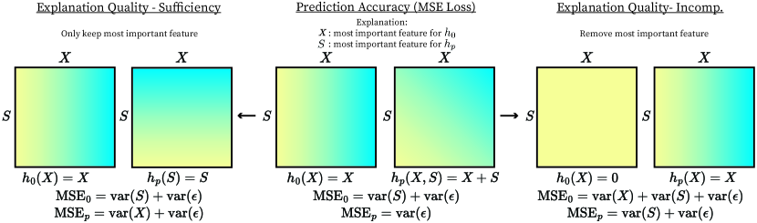
Figure 5: For a linear model, absence of benefit in explanation quality means that there is also an absence of benefit in prediction accuracy, as illustrated here (see Theorem 4.2). We consider a linear model $Y=X+S+\epsilon$, with $h_{0}$ and $h_{p}$ Bayes optimal regressors. In this example, absence of benefit of personalization for the explanation quality, $\text{BoP-X}^{\text{suff}}=0$ evaluated in terms of sufficiency (left column) means: $\Delta\text{MSE}_{0}=\Delta\text{MSE}_{p}\Rightarrow\text{var}(X)=0$. Then, absence of benefit of personalization for the explanation quality, $\text{BoP-X}^{\text{comp}}=0$ evaluated in terms of comprehensiveness (right column) means: $\Delta\text{MSE}_{0}=\Delta\text{MSE}_{p}\Rightarrow\text{var}(S)=\text{var}(X)\Rightarrow\text{var}(S)=0$. This allows us to conclude that, in terms of prediction accuracy (middle column): $\text{MSE}_{0}=\text{MSE}_{p}$ and hence there is also no benefit of personalization in prediction :$\text{BoP-P}=0$.

Proof.

A Bayes optimal regressor using a subset of variables from indices in $J\subseteq[1,\ldots,t+k]$ would be given as:

$$\hat{y}=h^{*}_{J}(\mathbf{x}_{J},\mathbf{s}_{J})=\sum_{\begin{subarray}{c}j\in J,\\ j\leq t\end{subarray}}\alpha_{j}x_{j}+\sum_{\begin{subarray}{c}j\in J,\\ j\geq t+1\end{subarray}}\alpha_{j}S_{j-t},$$ (20)

where $h^{*}_{J}$ represents an Bayes optimal regressor for the given subset $J$, and $\mathbf{x}_{J}$ and $\mathbf{x}_{J}$ are sub-vectors of $\mathbf{x}$ and $\mathbf{s}$, using the indices in $J$. Then, the MSE of $h^{*}_{J}$ is given as:

$$\text{MSE}(h^{*}_{J})=\sum_{\begin{subarray}{c}j\in\setminus J,\\ j\leq t\end{subarray}}\alpha_{j}^{2}\text{Var}(X_{j})+\sum_{\begin{subarray}{c}j\in\setminus J,\\ j\geq t+1\end{subarray}}\alpha_{j}^{2}\text{Var}(S_{j-t}),$$ (21)

where $\setminus J$ is a shorthand notation for $[1,\ldots t+k]\setminus J$. By combining (20) and (21), we can obtain:

$$\text{MSE}(h_{0}) =\sum_{j=t+1}^{t+k}\alpha_{j}^{2}\text{Var}(S_{t+j})+\text{Var}(\epsilon),$$ (22)

$$\text{MSE}(h_{p}) =\text{Var}(\epsilon).$$ (23)

We define $J_{0}$ and $J_{p}$ as a set of important features for $h_{0}$ and $h_{p}$. Note that $J_{0}$ and $J_{p}$ are the same across all samples for the additive model. Then, for regressors for sufficiency, we can write the MSE as:

$$\text{MSE}(h_{0,J}) =\sum_{\begin{subarray}{c}j\in\setminus J_{0},\\ j\leq t\end{subarray}}\alpha_{j}^{2}\text{Var}(X_{t})+\sum_{j=t+1}^{t+k}\alpha_{j}^{2}\text{Var}(S_{j-t})+\text{Var}(\epsilon)$$ (24)

$$\text{MSE}(h_{p,J}) =\sum_{\begin{subarray}{c}j\in\setminus J_{p},\\ j\leq t\end{subarray}}\alpha_{j}^{2}\text{Var}(X_{t})+\sum_{\begin{subarray}{c}j\in\setminus J_{p},\\ j\geq t+1\end{subarray}}\alpha_{j}^{2}\text{Var}(S_{j-t})+\text{Var}(\epsilon).$$ (25)

Similarly, for regressors for incomprehensiveness, MSE can be written as:

$$\text{MSE}(h_{0,\setminus J}) =\sum_{\begin{subarray}{c}j\in J_{0},\\ j\leq t\end{subarray}}\alpha_{j}^{2}\text{Var}(X_{t})+\sum_{j=t+1}^{t+k}\alpha_{j}^{2}\text{Var}(S_{j-t})+\text{Var}(\epsilon),$$ (26)

$$\text{MSE}(h_{p,\setminus J}) =\sum_{\begin{subarray}{c}j\in J_{p},\\ j\leq t\end{subarray}}\alpha_{j}^{2}\text{Var}(X_{t})+\sum_{\begin{subarray}{c}j\in J_{p},\\ j\geq t+1\end{subarray}}\alpha_{j}^{2}\text{Var}(S_{j-t})+\text{Var}(\epsilon).$$ (27)

Then, our assumption of $\text{BoP-X}=0$ for sufficiency becomes:

$$\text{MSE}(h_{0})-\text{MSE}(h_{0,J}) =\text{MSE}(h_{p})-\text{MSE}(h_{p,J}).$$ (28)

We can expand $\text{MSE}(h_{0})-\text{MSE}(h_{0,J})$ as:

$$\text{MSE}(h_{0})-\text{MSE}(h_{0,J}) =\text{MSE}(h_{0})\left(1-\frac{\text{MSE}(h_{0,J})}{\text{MSE}(h_{0})}\right)$$

$$=\text{MSE}(h_{0})\left(1-\frac{\text{Var}(\setminus J_{0})+\text{Var}(S)+\text{Var}(\epsilon)}{\text{Var}(S)+\text{Var}(\epsilon)}\right)$$

$$=\text{MSE}(h_{0})\frac{\text{Var}(\setminus J_{0})}{\text{Var}(S)+\text{Var}(\epsilon)}$$

$$=\text{MSE}(h_{0})\frac{\text{Var}(J_{0})+\text{Var}(\setminus J_{0})}{\text{Var}(S)+\text{Var}(\epsilon)}\frac{\text{Var}(\setminus J_{0})}{\text{Var}(J_{0})+\text{Var}(\setminus J_{0})},$$ (29)

where we use the shorthand notations:

$$\text{Var}(J_{0}) =\sum_{\begin{subarray}{c}j\in J_{0},\\ j\leq t\end{subarray}}\alpha_{j}^{2}\text{Var}(X_{t}),$$

$$\text{Var}(\setminus J_{0}) =\sum_{\begin{subarray}{c}j\in\setminus J_{0},\\ j\leq t\end{subarray}}\alpha_{j}^{2}\text{Var}(X_{t}),$$

$$\text{Var}(S) =\sum_{j=t+1}^{t+k}\alpha_{j}^{2}\text{Var}(S_{t+j}).$$

Further, note that

$$\text{Var}(J_{0})+\text{Var}(\setminus J_{0})=\sum_{\begin{subarray}{c}j\in J_{0},\\ j\leq t\end{subarray}}\alpha_{j}^{2}\text{Var}(X_{t})+\sum_{\begin{subarray}{c}j\in\setminus J_{0},\\ j\leq t\end{subarray}}\alpha_{j}^{2}\text{Var}(X_{t})=\sum_{j=1}^{t}\alpha_{j}^{2}\text{Var}(X_{j})=\text{Var}(X).$$

Defining $M(h_{0})\triangleq\text{MSE}(h_{0})\frac{\text{Var}(X)}{\text{Var}(S)+\text{Var}(\epsilon)}$ and $r_{0}\triangleq\frac{\text{Var}(J_{0})}{\text{Var}(J_{0})+\text{Var}(\setminus J_{0})}$, we further simplify (29) as:

$$\text{MSE}(h_{0})-\text{MSE}(h_{0,J})=M(h_{0})(1-r_{0}).$$ (30)

Through a similar process, we can simpilfy $\text{MSE}(h_{p})-\text{MSE}(h_{p,J})$ as:

$$\text{MSE}(h_{p})-\text{MSE}(h_{0,p})=M(h_{p})(1-r_{p}),$$ (31)

where $M(h_{p})\triangleq\frac{\text{Var}(X)+\text{Var}(S)}{\text{Var}(\epsilon)}\text{MSE}(h_{p})$ and $r_{p}\triangleq\frac{\text{Var}(J_{p})}{\text{Var}(J_{p})+\text{Var}(\setminus J_{p})}$ Using (30) and (31), we arrive at:

$$M(h_{0})(1-r_{0})=M(h_{p})(1-r_{p}).$$ (32)

By taking similar steps using comprehensiveness, we can derive:

$$M(h_{0})r_{0}=M(h_{p})r_{p}.$$ (33)

By combining (32) and (33), we can conclude that:

$$\frac{r_{0}}{r_{p}}=\frac{1-r_{0}}{1-r_{p}}\implies r_{0}=r_{p}.$$

Plugging this back to (32), we get: $M(h_{0})=M(h_{p})$. Now, let us assume that $\text{BoP-P}>0$, and prove it by contradiction. Comparing (22) and (23), we can deduce that $\text{BoP-P}>0$ means $\text{Var}(S)>0$. Expanding $M(h_{0})=M(h_{p})$, we get:

$$\text{MSE}(h_{0})\frac{\text{Var}(X)}{\text{Var}(S)+\text{Var}(\epsilon)} =\frac{\text{Var}(X)+\text{Var}(S)}{\text{Var}(\epsilon)}\text{MSE}(h_{p}),$$

$$\text{MSE}(h_{p}) =\frac{\text{Var}(X)}{\text{Var}(X)+\text{Var}(S)}\frac{\text{Var}(\epsilon)}{\text{Var}(S)+\text{Var}(\epsilon)}\text{MSE}(h_{0}),$$

$$=\frac{\text{Var}(X)}{\text{Var}(X)+\text{Var}(S)}\text{MSE}(h_{p}).$$

Since $\text{Var}(S)>0$, this equality cannot hold. This concludes that $\text{BoP-P}=0$. We can make the same claim with similar logic for a classifier where $Y$ is given as:

$$Y=\mathds{1}(\alpha_{1}X_{1}+\cdots\alpha_{t}X_{t}+\alpha_{t+1}S_{1}+\cdots+\alpha_{t+k}S_{k}+\epsilon>0).$$ (34)

∎

Appendix F Max attributes

Proof.

If $\min\max P_{e}\leq 1/2$, then:

$$1-\frac{1}{2\sqrt{d}}\exp\left(\frac{m\epsilon^{2}}{2\sigma^{2}}\right)\leq\min\max P_{2}\leq 1/2$$ (35)

Or equivalently, if $\min\max P_{e}\leq 1/2$, then:

$$\frac{1}{\sqrt{d}}\exp\left(\frac{m\epsilon^{2}}{2\sigma^{2}}\right)\geq 1$$ (36)

Given the number of groups $d=2^{k}$, the number of samples per group $m=n/d$, the total number of samples $n=10^{4}$ and the threshold of $\epsilon=0.01$, we get:

$$\phi(k)=1-\frac{1}{2^{k/2+1}}\exp\left(\frac{\frac{10^{4}}{2^{k}}\times 0.0001}{2\sigma^{2}}\right)=1-\frac{1}{2^{k/2+1}}\exp\left(\frac{1}{2^{k+1}\sigma^{2}}\right)$$ (37)

We prove that this function is an increasing function in $k$. Indeed, consider the auxiliary function $f(x)=\frac{1}{2\sqrt{x}}\exp(\frac{a}{x})$. Its derivative is $f^{\prime}(x)=-\frac{\exp(\frac{a}{x})(2a+x)}{4x^{5/2}}$. For $x,a>0$, we have: $f^{\prime}(x)<0$, i.e., $f$ is a monotonically decreasing function. Consequently, $1-f$ is a monotonically increasing function. Thus, the function $k\rightarrow 1-f(2^{k})$ with $a=\frac{1}{2\sigma^{2}}$ is a monotonically increasing function of $k>0$. ∎

Appendix G MIMIC-III Experiment Results

Below is all supplementary material for the MIMIC-III experiment. This includes BoP distribution plots and plots showing how incomprehensiveness and sufficiency change over the number of features removed.

G.1 Experiment Plots

In the following section, we show supplementary plots for the regression task on the auditing dataset. We show the distribution of the BoP across participants for all three metrics we evaluate. We overlay Laplace and Gaussian distributions to see which fit the individual BoP distribution best, illustrating that prediction and incomprehensiveness are best fit by Laplace distributions and sufficiency by a Gaussian distribution. Additionally, we show how incomprehensiveness and sufficiency change for the number of important attributes $r$ that are kept are removed.

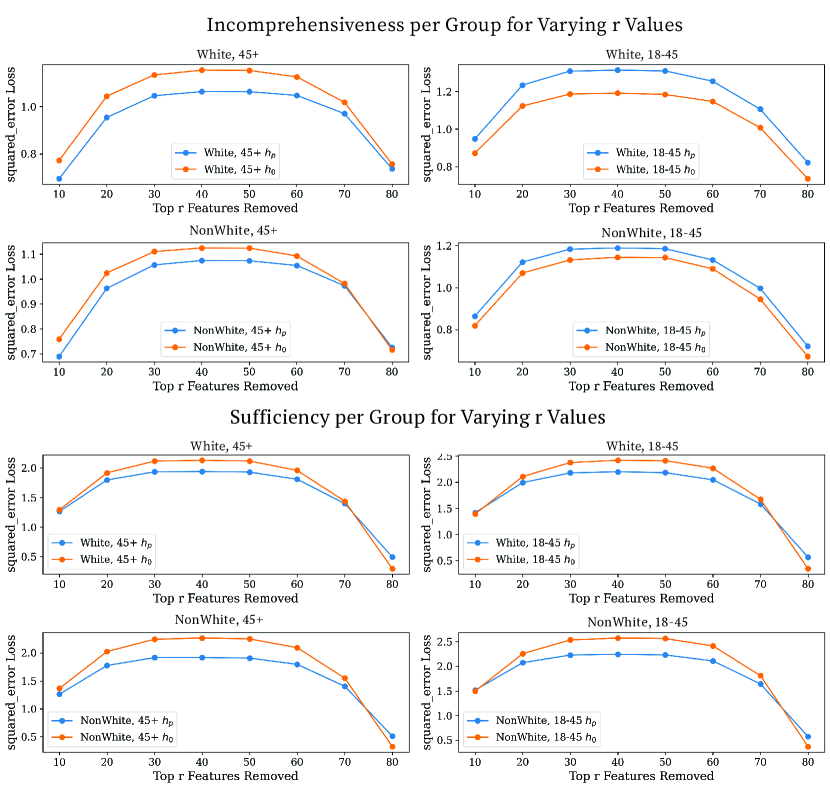
Figure 9: Values of Sufficiency and Incomprehensiveness across varying $r$ top features selected using the square error loss function. Values are found for $h_{0}$ and $h_{p}$.

References

• Agarwal et al. (2019) Agarwal, A., Dudík, M., and Wu, Z. S. Fair regression: Quantitative definitions and reduction-based algorithms, 2019. URL https://arxiv.org/abs/1905.12843.
• Balagopalan et al. (2022) Balagopalan, A., Zhang, H., Hamidieh, K., Hartvigsen, T., Rudzicz, F., and Ghassemi, M. The road to explainability is paved with bias: Measuring the fairness of explanations. In 2022 ACM Conference on Fairness, Accountability, and Transparency, FAccT ’22. ACM, June 2022. doi: 10.1145/3531146.3533179. URL http://dx.doi.org/10.1145/3531146.3533179.
• Berk et al. (2017) Berk, R., Heidari, H., Jabbari, S., Joseph, M., Kearns, M., Morgenstern, J., Neel, S., and Roth, A. A convex framework for fair regression, 2017. URL https://arxiv.org/abs/1706.02409.
• Calders et al. (2013) Calders, T., Karim, A., Kamiran, F., Ali, W., and Zhang, X. Controlling attribute effect in linear regression. 2013 IEEE 13th International Conference on Data Mining, pp.  71–80, 2013. URL https://api.semanticscholar.org/CorpusID:16541789.
• Dasgupta et al. (2022) Dasgupta, S., Frost, N., and Moshkovitz, M. Framework for evaluating faithfulness of local explanations, 2022. URL https://arxiv.org/abs/2202.00734.
• DeYoung et al. (2020) DeYoung, J., Jain, S., Rajani, N. F., Lehman, E., Xiong, C., Socher, R., and Wallace, B. C. ERASER: A benchmark to evaluate rationalized NLP models. In Jurafsky, D., Chai, J., Schluter, N., and Tetreault, J. (eds.), Proceedings of the 58th Annual Meeting of the Association for Computational Linguistics, pp.  4443–4458, Online, July 2020. Association for Computational Linguistics. doi: 10.18653/v1/2020.acl-main.408. URL https://aclanthology.org/2020.acl-main.408.
• Dwork & Ilvento (2019) Dwork, C. and Ilvento, C. Fairness under composition. Schloss Dagstuhl – Leibniz-Zentrum für Informatik, 2019. doi: 10.4230/LIPICS.ITCS.2019.33. URL https://drops.dagstuhl.de/entities/document/10.4230/LIPIcs.ITCS.2019.33.
• Dwork et al. (2011) Dwork, C., Hardt, M., Pitassi, T., Reingold, O., and Zemel, R. Fairness through awareness, 2011. URL https://arxiv.org/abs/1104.3913.
• Flack et al. (2003) Flack, J. M., Ferdinand, K. C., and Nasser, S. A. Epidemiology of hypertension and cardiovascular disease in african americans. The Journal of Clinical Hypertension, 5(1):5–11, 2003.
• Fukuchi et al. (2013) Fukuchi, K., Kamishima, T., and Sakuma, J. Prediction with model-based neutrality. In ECML/PKDD, 2013. URL https://api.semanticscholar.org/CorpusID:6964544.
• Gursoy & Kakadiaris (2022) Gursoy, F. and Kakadiaris, I. A. Error parity fairness: Testing for group fairness in regression tasks, 2022. URL https://arxiv.org/abs/2208.08279.
• Hardt et al. (2016) Hardt, M., Price, E., and Srebro, N. Equality of opportunity in supervised learning, 2016. URL https://arxiv.org/abs/1610.02413.
• Huang et al. (2024) Huang, B., Dalakoti, M., and Lip, G. Y. H. How far are we from accurate sex-specific risk prediction of cardiovascular disease? One size may not fit all. Cardiovascular Research, 120(11):1237–1238, 06 2024. ISSN 0008-6363. doi: 10.1093/cvr/cvae135. URL https://doi.org/10.1093/cvr/cvae135.
• Jacovi & Goldberg (2020) Jacovi, A. and Goldberg, Y. Towards faithfully interpretable NLP systems: How should we define and evaluate faithfulness? In Jurafsky, D., Chai, J., Schluter, N., and Tetreault, J. (eds.), Proceedings of the 58th Annual Meeting of the Association for Computational Linguistics, pp.  4198–4205, Online, July 2020. Association for Computational Linguistics. doi: 10.18653/v1/2020.acl-main.386. URL https://aclanthology.org/2020.acl-main.386.
• Johnson et al. (2016) Johnson, A. E., Pollard, T. J., Shen, L., Lehman, L.-w. H., Feng, M., Ghassemi, M., Moody, B., Szolovits, P., Anthony Celi, L., and Mark, R. G. Mimic-iii, a freely accessible critical care database. Scientific data, 3(1):160035–160035, 2016. ISSN 2052-4463.
• Kroenke et al. (2001) Kroenke, K., Spitzer, R. L., and Williams, J. B. W. The phq-9: Validity of a brief depression severity measure. Journal of General Internal Medicine, 16:606–613, 2001.
• Lyu et al. (2024) Lyu, Q., Apidianaki, M., and Callison-Burch, C. Towards faithful model explanation in nlp: A survey, 2024. URL https://arxiv.org/abs/2209.11326.
• Mehrabi et al. (2022) Mehrabi, N., Morstatter, F., Saxena, N., Lerman, K., and Galstyan, A. A survey on bias and fairness in machine learning, 2022. URL https://arxiv.org/abs/1908.09635.
• Monteiro Paes et al. (2022) Monteiro Paes, L., Long, C., Ustun, B., and Calmon, F. On the epistemic limits of personalized prediction. Advances in Neural Information Processing Systems, 35:1979–1991, 2022.
• Mosca et al. (2011) Mosca, L., Barrett-Connor, E., and Wenger, N. Sex/gender differences in cardiovascular disease prevention what a difference a decade makes. Circulation, 124:2145–54, 11 2011. doi: 10.1161/CIRCULATIONAHA.110.968792.
• Nauta et al. (2023) Nauta, M., Trienes, J., Pathak, S., Nguyen, E., Peters, M., Schmitt, Y., Schlötterer, J., van Keulen, M., and Seifert, C. From anecdotal evidence to quantitative evaluation methods: A systematic review on evaluating explainable ai. ACM Computing Surveys, 55(13s):1–42, July 2023. ISSN 1557-7341. doi: 10.1145/3583558. URL http://dx.doi.org/10.1145/3583558.
• Obermeyer et al. (2019) Obermeyer, Z., Powers, B., Vogeli, C., and Mullainathan, S. Dissecting racial bias in an algorithm used to manage the health of populations. Science, 366(6464):447–453, October 2019. ISSN 1095-9203. doi: 10.1126/science.aax2342. URL http://dx.doi.org/10.1126/science.aax2342.
• Paulus et al. (2016) Paulus, J., Wessler, B., Lundquist, C., Yh, L., Raman, G., Lutz, J., and Kent, D. Field synopsis of sex in clinical prediction models for cardiovascular disease. Circulation: Cardiovascular Quality and Outcomes, 9:S8–S15, 02 2016. doi: 10.1161/CIRCOUTCOMES.115.002473.
• Paulus et al. (2018) Paulus, J., Wessler, B., Lundquist, C., and Kent, D. Effects of race are rarely included in clinical prediction models for cardiovascular disease. Journal of General Internal Medicine, 33, 05 2018. doi: 10.1007/s11606-018-4475-x.
• Pessach & Shmueli (2022) Pessach, D. and Shmueli, E. A review on fairness in machine learning. ACM Comput. Surv., 55(3), feb 2022. ISSN 0360-0300. doi: 10.1145/3494672. URL https://doi.org/10.1145/3494672.
• Pérez-Suay et al. (2017) Pérez-Suay, A., Laparra, V., Mateo-García, G., Muñoz-Marí, J., Gómez-Chova, L., and Camps-Valls, G. Fair kernel learning, 2017. URL https://arxiv.org/abs/1710.05578.
• Simonyan et al. (2014) Simonyan, K., Vedaldi, A., and Zisserman, A. Deep inside convolutional networks: Visualising image classification models and saliency maps, 2014. URL https://arxiv.org/abs/1312.6034.
• Smilkov et al. (2017) Smilkov, D., Thorat, N., Kim, B., Viégas, F., and Wattenberg, M. Smoothgrad: removing noise by adding noise, 2017. URL https://arxiv.org/abs/1706.03825.
• Sundararajan et al. (2017) Sundararajan, M., Taly, A., and Yan, Q. Axiomatic attribution for deep networks, 2017. URL https://arxiv.org/abs/1703.01365.
• Suriyakumar et al. (2023) Suriyakumar, V. M., Ghassemi, M., and Ustun, B. When personalization harms: Reconsidering the use of group attributes in prediction, 2023. URL https://arxiv.org/abs/2206.02058.
• Yin et al. (2022) Yin, F., Shi, Z., Hsieh, C.-J., and Chang, K.-W. On the sensitivity and stability of model interpretations in nlp, 2022. URL https://arxiv.org/abs/2104.08782.
• Yuan et al. (2022) Yuan, H., Yu, H., Gui, S., and Ji, S. Explainability in graph neural networks: A taxonomic survey, 2022. URL https://arxiv.org/abs/2012.15445.