Simultaneous reconstruction of two potentials for a nonconservative Schrödinger equation with dynamic boundary conditions
Abstract
In this article, we consider an inverse problem involving the simultaneous reconstruction of two real valued potentials for a Schödinger equation with mixed boundary conditions: a dynamic boundary condition of Wentzell type and a Dirichlet boundary condition. The main result of this paper is a Lipschitz stability estimate for such potentials from a single measurement of the flux. This result is deduced using the Bukhgeim-Klibanov method and a suitable Carleman estimate where the weight function depends on Minkowski’s functional.
Keywords: Schrödinger equation, inverse problem, dynamic boundary conditions, Carleman estimates.
MSC (2020): 35J10; 35R25; 35R30; 49M41.
1 Introduction
Let , , be a bounded domain with smooth boundary . We assume that with and are two closed subsets satisfying . Unless explicitly stated otherwise, all of the function spaces discussed in this paper will concern complex-valued functions.
We introduce the operators and given by
| (1.1) |
and
| (1.2) |
where denotes the imaginary unit, , and are vector valued functions defined in and on , respectively. Moreover, denotes the normal derivative associated to the outward normal of , is the tangential gradient and is the Laplace Beltrami operator.
In this article, we will consider the following nonconservative Schrödinger equation with dynamic boundary conditions:
| (1.3) |
where is the source term, and are the potentials and is the initial data.
We recall that, under the following assumptions on , , and suitable assumptions on (see Section 2) the problem (1.3) has a unique weak solution. Moreover, there exists a positive constant such that the solution of (1.3) satisfies
In this paper, we are interested in an coefficient inverse problem associated to the Schrödinger equation with dynamic boundary conditions. More precisely, we consider the following:
Coefficient Inverse Problem (CIP): Is it possible to retrieve from a measurement of the normal derivative on (), where is the solution of (1.3) associated to ?
We point out that our goal is the study of dependence of solutions of system (1.3) with respect to the potentials and . For this reason, we ignore for instance the dependence of the solutions of (1.3) with respecto to the initial conditions and source terms. Besides, to emphasize this fact, sometimes we shall write
In this direction, the following questions naturally arise:
-
•
Uniqueness: Does the inequality on imply in and on ?
-
•
Stability: Is it possible to estimate and , by a suitable norm of on ?
-
•
Reconstruction formula: Can we find an algorithm to compute the potentials and by partial knowledge of on ?
In this article, we focus on the stability and reconstruction aspects of (CIP), properties derived under specific assumptions. Naturally, the stability result also ensures uniqueness.
We also consider the same inverse problem for a one-dimensional version of (1.3), which reads as follows.
| (1.4) |
where , , and . Here, the pair stands for the state of the system (1.4).
Our work is organized into two main parts. First, we derive a new Carleman estimate for the Schrödinger operator with dynamic boundary conditions and use these estimates to apply the Bukhgeim-Klibanov method. Second, based on these results, we develop a constructive and iterative algorithm to determine the coefficients using specific additional data. This involves analyzing an appropriate functional derived from a data assimilation problem and showing the existence of a unique minimizer in a suitable space, from where we obtain the convergence of the iterative algorithm, which is adapted from the Carleman-based approach introduced in [3].
1.1 Related references
The first application of Carleman estimates in the context of inverse problems is due to Bukhgeim and Klibanov in 1981 in [9]. In this article, the authors proved Hölder stability results using a local Carleman estimate for complactly supported functions. After that, this method was slightly modified by Puel and Yamamoto in [26] by using a global Carleman estimate for the wave equation, allowing to obtain Lipschitz stability results for the Inverse source problem. See also [16], [17], [22] and [10] for some related inverse problems for the wave equation and systems.
The Carleman-based reconstruction algorithm (CbRec for short) was introduced in [3] to study the reconstruction of the time independent potential of the wave equation posed in a bounded domain with Dirichlet boundary condition, with measurements on the flux of the solution in an appropriate subset of the boundary. This approach is inspired in the ideas given in [21] and [20] under additional assumptions. In [3], It is proved that this algorithm globally converges to the exact solution of the inverse problem for the wave equation, i.e., it converges to the unknown potential independently of the initial guest of the algorithm.
Unfortunately, the Carleman weights of the wave equation involves two exponential functions, which generates drawbacks in numerical simulations. In fact, in [14] the authors reconstructed numerically a control for the wave equation with a quadratic functional involving exponential weights with small values of the Carleman parameters, i.e., and . To avoid this problem, in [4] the same authors studied the same problem, but this time a Carleman estimate was obtained by using a one parameter weight function. This allows to use the CbRec algorithm to reconstruction the unknown potential but the price to pay is additional observations are needed. These ideas have been studied to recover the speed coefficient of the wave in [5] for the wave equation and in [8] to reconstruct a spatial part of the source term in a reaction-diffusion equation. More recently, in [2] the CbRec algorithm has been implemented to address an inverse problem for the wave equation in a tree shaped network.
Concerning inverse problems for the Schrödinger equation, we mention the work [7], where the authors consider a coefficient inverse problem of recovering the zeroth order potential of the Schrödinger equation (with ) with Dirichlet boundary conditions . Here, a Carleman estimate for the Schrödinger operator is proved using geometric conditions. Moreover, using the Bukhgeim-Klibanov method, a Lipschitz stability estimate is obtained. After that, in [6] consider a similar inverse problem but with being a discontinuous continuous function. Once again, with a new Carleman estimate at hand, Lipschitz stability results have been obtained for such inverse problem. More recently, in [18] an inverse source problem for general Schrödinger equation is studied. In that article, the authors prove stability results when no geometric conditions are assumed on the domain. The results relies on a different approach which depends on a transformation of the Schrödinger equation to an elliptic one. The key point here is such transformation is defined by a solution to a controllability problem for the one-dimensional Schrödinger equation. On the other hand, we refer to [23], [24] and [28] on the study of well-posedness, stability and pointwise Carleman estimates for nonconservative Schrödinger equations with different boundary conditions.
Only a few papers have been devoted to the study of inverse problems for PDEs with dynamic boundary conditions. In [11], the authors studies the identification of initial data for the heat equation with dynamic boundary condition. Recently, in [12] the authors studied controllability issues and Inverse problem for the wave equation with kinetic boundary conditions. The findings of this article improve those obtained in [15] with an additional geometric assumption. The key point used there is a new Carleman estimate for the wave operator with kinetic boundary conditions, where the associated weight function depends on the Minkowski functional, similar to those used in [25]. More recently, in [13] the authors studied an inverse problem where the goal is to identity two spatial-temporal source terms for the Schrödinger equation with dynamic boundary conditions from final time measurements. To deal with it, the authors adopt a Tikhonov regularization strategy and analyze the properties of such functional. In particular, the existence and uniqueness of the solutions is investigated. In addition, some numerical experiments are given in one-dimensional case.
To the best of our knowledge, this is the first time that (CIP) is considered for a non conservative Schrödinger equation with dynamic boundary conditions.
1.2 Setting
In this section, we set up the notation and terminology used in this paper. Firstly, we consider the set as an -dimensional compact Riemannian submanifold equipped by the Riemannian metric induced by the natural embedding . We point out that it is possible to define the differential operators on in terms of the Riemannian metric . However, for the purposes of this article, it will be enough to use the most important properties of the underlying operators and spaces. The details can be found, for instance, in [19] and [27]. For the sake of completeness, we recall some of those properties.
The tangential gradient of at each point can be seen as the projection of the standard Euclidean gradient onto the tangent space of , where is the trace of on , i.e.,
where on and is the normal derivative associated to the outward normal . In this way, the tangential divergence in is given by
Moreover, denotes the Laplace-Beltrami operator, which satisfies for all . In particular, the surface divergence theorem holds:
| (1.5) |
For , we define the Banach spaces endowed by their natural norms. In particular, the space is a the Hilbert space endowed by the scalar product
Moreover, for , we consider the space
which is a closed subspace of the Sobolev space . Moreover, for , we set
We point out that, thanks to the Trace Theorem and Poincaré’s inequality, is a Hilbert space in endowed by
for all .
1.3 Main results
Now, we give a definition related with the geometric hypothesis we will assume for the interior boundary.
Definition 1.1.
An open, bounded and convex set , is said to be strongly convex if is of class and all the principal curvatures are strictly positive functions on .
Remark 1.2.
We point out that a strongly convex set is geometrically strictly convex, in the sense that it has, at each of its boundary points, a supporting hyperplane with exactly one contact point.
We will consider the following
-
(A1)
(Geometric assumption) We suppose that can be written in the form , where is strongly convex and is an open set with .
Without loss of generality, we can assume that . Otherwise, take and apply a translation by .
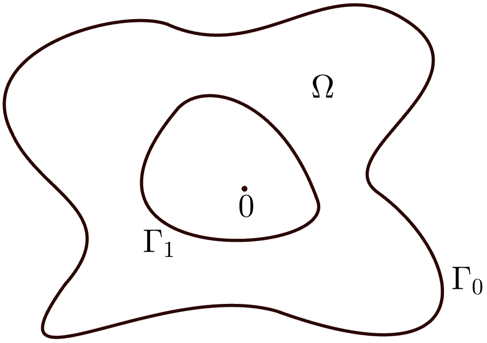
From now on, we write , with . We define, for each ,
| (1.6) |
Since is open and convex, we have that and are well-defined and that on . In order to guarantee enough regularity for our purposes, we consider the following assumption:
-
(A2)
(Regularity of the boundary ) We assume that the boundary has a regular parametrization, i.e., the mapping is a diffeomorfism.
Then we have (see Proposition 3.1 of [25]) that , in , and there exists such that
Define , which is our observation region, as
| (1.7) |
Now, for and , we introduce
and define the set of potentials as
| (1.8) |
Now, we state the main result of this article, concerning (CIP).
Theorem 1.3.
Consider the assumptions (A1) and (A2). Define the function given in (1.6). Moreover, for given we consider . Assume that and satisfy the condition
| (1.9) |
In addition, suppose that
| (1.10) |
and the initial data and are real valued functions satisfying
| (1.11) |
for some positive constant . Then, there exists a constant such that if , then the following inequality holds
| (1.12) |
for all .
We point out that inequality (1.12) establishes a Lipschitz stability result for the inverse problem (CIP) for the Schrödinger equation with dynamic boundary conditions from (partial) boundary observations given in .
Remark 1.4.
Before going further, some remarks are in order:
- •
- •
- •
Remark 1.5.
Hypothesis (1.10) is a typical technical condition for obtaining stability in a one-measurement inverse problem. It can be satisfied by ensuring the system has sufficiently regular data.
We can also formulate a stability result for the one-dimensional model (1.4). To do this, for , we define the spaces
endowed by its natural norm and for , we also set the subspace
Then, we have the following result:
Theorem 1.6.
Given , set . Suppose that , , and are chosen such that
where and are real valued functions which also satisfy
for some constant . Then, there exists a constant such that if , then the following inequality holds
for all .
1.4 Outline of the paper
The rest of the article is organized as follows. In Section 2 we review some basic results on the existence and uniqueness of solutions to the Schrödinger equation with dynamic boundary conditions. We also present a Carleman estimate for these systems with observations on part of the boundary. In Section 3, we prove the stability of the inverse problem discussed in Theorem 1.3. Section 4 focuses on the convergence of the reconstruction algorithm. Finally, Section 5 provides concluding remarks and additional observations.
2 Preliminaries
In this section, we present existence, uniqueness, and other basic properties of the Schrödinger equation with dynamic boundary conditions. Additionally, we present a Carleman estimate for this system, considering observations on a subset of the boundary.
2.1 Existence and uniqueness of solutions and hidden regularity
Given , we consider the problem
| (2.1) |
Concerning the existence and uniqueness of (2.1), we have the following result:
Proposition 2.1 (Proposition 2.1 [25]).
Suppose that , . Furthermore, suppose that such that on , and . Then, the weak solution belongs to . Besides, there exists such that
The following results relies on the existence and uniqueness of weak solutions of (2.1) for more regular data.
Proposition 2.2 (Proposition 2.2 [25]).
Suppose that and . In addition, assume that satisfies the following conditions
We also assume that satisfies . Then, the weak solution of (2.1) belongs to with . Moreover, there exists such that
The next result establishes a hidden regularity result for the Schrödinger equation with dynamic boundary conditions.
Proposition 2.3 (Proposition 2.5 [25]).
We can also obtain existence and uniqueness results for the one-dimensional Schrödinger equation with dynamic boundary conditions as well as a hidden regularity result for the normal derivative. These results can be achieved using multiplier techniques.
2.2 A Carleman estimate for the Schrödinger equation with dynamic boundary conditions
For and , we introduce the operators
| (2.3) |
and
| (2.4) |
Moreover, due to the last identity, from now on we shall write instead of on . Firstly, define the operators
and
Theorem 2.4.
3 Proof of the stability result
This section is devoted to prove Theorem 1.3. In order to do this, we need to establish a suitable Carleman estimate for the Schrödinger operator with dynamic boundary conditions.
3.1 An auxiliar Carleman estimate
We start with the following result.
Theorem 3.1.
Proof.
As usual, we argue by density, i.e., we consider such that on and on . We shall prove that the terms
are bounded by above by the left-hand side of (2.5). To do this, we consider
where denotes the imaginary part of a complex number and . After integration by parts, taking into account that on and in , we deduce that
| (3.2) |
On the other hand, using the Surface Divergence Theorem (1.5) and the fact that , we see that
| (3.3) |
By definitions of and , we see that
| (3.5) |
3.2 Proof of the main result
Now, we are able to prove the Theorem 1.3.
Proof.
We fix and define
| (3.7) |
where and are the solutions of (1.3) associated to the potentials and , respectively. We also define
| (3.8) |
Then, satisfies
Next, we set . Then, satisfies
Now, we define
We also extend by for , and in an analogous way for . We denote these extensions by the same symbols. Since and are real valued, we have that satisfies the corresponding system posed in . In particular, this implies that and . Thus, by regularity assumption 1.10 we deduce that
| (3.9) |
Now, applying Theorem 3.1 to we obtain
| (3.10) | ||||
On the other hand, by (1.11) we have
| (3.11) |
Then, from (3.9) we deduce the existence of such that
| (3.12) | ||||
Moreover, we see that
Thus, taking and large enough if it is necessary we can absorb the first two terms of (3.13). Additionally, by (3.11) we deduce that
| (3.14) | ||||
for all and . Finally, we fix and and we come back to the original variables in (3.7) and (3.8). Finally, since the weights and are bounded, we deduce that
and the proof of Theorem 1.3 is complete. ∎
4 Convergence results of CbRec
Now, we shall give an algorithm to reconstruct the potentials on (1.3). In order to do that, we introduce an auxiliary functional based on the weights (2.2) and the Carleman estimate obtained in Theorem 3.1.
4.1 An auxiliary functional and some properties
We fix , and choose according to Theorem 3.1. Then, for all , we introduce the functional
| (4.1) | ||||
where and , with and defined in (1.1) and (1.2) and
endowed by the norm
| (4.2) | ||||
We point out that depends on the parameter . However, to simply notation, we just write instead of . From now on, we shall consider the unconstrained problem
| (4.3) |
Theorem 4.1.
For , and given by Theorem 3.1, we consider the functional defined on , for all . Then,
-
(a)
The problem (4.3) admits a unique minimizer . Moreover, there exists a constant independent of such that
(4.4) -
(b)
The minimizer satisfies the associated Euler-Lagrange equation
(4.5) where denotes the real part of a complex number.
-
(c)
If , and is the corresponding minimizer of for , then we have the following estimate
(4.6) for some constant independent of .
Proof.
-
(a)
Clearly, the functional is clearly continuous and strictly convex. In order to prove that is coercive, we point out that
(4.7) (4.8) where in (4.8) we have used Young’s inequality in the last step and is given in (4.2). This implies that is coercive and therefore admits a unique minimizer . In order to prove (4.4), since and (4.7) we have
Then, by Young’s inequality, for all , there exists a constant such that
Thus, taking small enough we conclude the proof of (4.4).
-
(b)
Direct from the fact that has a unique minimizer.
- (c)
∎
4.2 A CbRec type algorithm
We now present an algorithm designed to reconstruct the potentials and . To do this, we fix and define the space defined in (1.8). Then, the algorithm reads as follows:
Initialization:
-
•
, or any guess .
Iteration: From to .
-
•
Step 1: Given , we set
where and are the solutions of (1.3) associated to the potentials and , respectively.
-
•
Step 2: Find the minimizer of the unconstrained problem
-
•
Step 3: Set
(4.12) -
•
Step 4: Finally, consider and , where the operators and are given by
Theorem 4.2.
Assume the hypotheses of Theorem 4.1. Additionally, suppose that
Remark 4.3.
Proof of Theorem 4.2.
In this section, we prove the convergence of the Algorithm 1. To do this, let and consider and . Then, is a solution of
| (4.15) |
where and are given by and , respectively. Then, we set
| (4.16) |
Note that . Therefore, by (4.16) the solution of (4.15) satisfies the Euler-Lagrange equation associated to the functional in (4.5) with and . Since admits a unique minimizer, corresponds to the minimum of .
Now, let be the minimizer of . Then, from inequality (4.6) we obtain
| (4.17) | ||||
On the other hand, since and are Lipschitz continuous functions and satisfy and , we have
and
5 Further comments and concluding remarks
In this paper, we have presented the coefficient inverse problem (CIP) for a Schrödinger equation with dynamic boundary conditions. We have provided a Lipschitz stability result and a reconstruction algorithm. The stability result was obtained applying the Bukhgeim-Klibanov method, while the reconstruction algorithm is inspired on the CbRec Algorithm proposed in [3]. Besides, both results strongly depends on a suitable Carleman estimate for the Schrödinger operator with dynamic boundary conditions with observations on the normal derivative obtained for these purposes.
The assumption (A1) plays an important role in our results. The strong convexity condition on the is given to define a weight function which is constant on the boundary . To the best of our knowledge, the case where is non strictly convex has not been considered yet in the context of the wave and Schrödinger equation with dynamic boundary conditions.
Our results depends also of the condition , where it is used to deduce the Carleman estimate for the Schrödinger operator. We mention that an analogous hypothesis also appeared in context of controllability of the wave equation with acoustic boundary conditions, see for instance [1] and [12]. In particular, in the case of an annulus, it is proved in [1] that in the case , the associated adjoint problem is not observable at any time (see Theorem 2.4 in that reference). However, as far as we know, the case remains open for the wave equation. The same questions can be considered for the corresponding Schrödinger system.
One of the main advantages of the proposed algorithm, in contrast to the Tikhonov regularization techniques, is the fact that it converges to the exact potential independent of the initial guess. The numerical implementation of CbRec type algorithm for Schrödinger equations is, as far as we known, unexplored. Even the numerical Schrödinger equation with dynamic boundary conditions has not been studied, as far as the authors know. However, it seems not to be a problem to show in numerical experiments that its behavior is sufficiently good, while the main difficulties are shown in the implementation of the functional minimization step, which is not surprising due to previous works in CbRec type algorithms for other equations, such as in [4, 8], where additional terms have to be added to the functional to be minimized, and filters have to be applied in intermediate steps of the algorithm. Both additional tasks in the algorithm have been considered by the authors of the mentioned works due to regularity issues and for dealing with noisy measurements and the propagation of them in numerical differentiation. These difficulties seem to be shown even in the case of Dirichlet boundary conditions. Since numerical aspects of the implementation seem to be a separate subject from the scope of this article, this will be investigated in a forthcoming work.
Acknowledgments
The second author has been partially supported by Fondecyt 1211292 and ANID Millennium Science Initiative Program, Code NCN19-161. The third author has been funded under the Grant QUALIFICA by Junta de Andalucía grant number QUAL21 005 USE.
Appendix A Carleman estimate for the 1-D Schrödinger equation with dynamic boundary conditions
In this section, we deduce a Carleman estimate for the one-dimensional Schrödinger equation with dynamic boundary conditions. We set and . Then, we consider the following problem:
Given a point , with , set for each and for we define the weight functions
| (A.1) |
with .
For and , we introduce the operators:
| (A.2) |
and
| (A.3) |
Besides, for and , consider the operators
| (A.4) | ||||
Then, we have the following Carleman estimate:
Lemma A.1.
Let and be the functions defined in (A.1). There exist , and such that for all and ,
| (A.5) | ||||
for all such that and with .
Proof.
We argue by density arguments. Therefore, we just write for all . The proof of Lemma A.1 can be divided into four steps:
Step 1: We compute the terms
Straightforward computations show that
where and are defined in (A.2) and (A.3), respectively, and .
Then, we have the following identity
| (A.6) | ||||
Step 2: Estimates in . In this step, we compute the terms
In the following, we shall use the formulas:
The first term is given by
Moreover, integration by parts yields
On the other hand, using that , for all , we have
If is a constant which satisfies
then we have
| (A.7) |
Now, the term can be computed as follows
Since , we have
On the other hand, after using integration by parts, the term can be written as:
Besides, using for all , we have
where we have used the fact that for all . Now, using the estimates and and Young’s inequality, for all , there exists such that
Thus, choosing small enough and taking sufficiently large, we deduce that
| (A.8) | ||||
Now, let us estimate the terms , for . Observe that can be written in the form
We point out that this term cannot be estimated directly. Indeed, this term will be eliminated when we summing up the , .
Now, after integration by parts in space, the term can be written as follows:
Now, integrating by parts in time and using the fact that , we have
Then, by Young’s inequality, for all , there exists such that
Moreover, is given by
where we have used integration by parts in time and .
Thus, considering these estimates, we obtain
| (A.9) | ||||
Now, adding inequalities (A.7), (A.8) and (A.9), choosing small enough and taking sufficiently large, we deduce that
| (A.10) | ||||
Step 3: In this step, we will compute the terms
Observe that
Moreover, after integration by parts, the term can be estimated as
Then, we conclude that
| (A.11) |
References
- [1] L. Baudouin, J. Dardé, S. Ervedoza, and A. Mercado. A unified strategy for observability of waves in an annulus with various boundary conditions. Math. Rep. (Bucur.), 24(74)(1-2):59–112, 2022.
- [2] L. Baudouin, M. de Buhan, E. Crépeau, and J. Valein. Carleman-Based Reconstruction Algorithm on a wave Network. working paper or preprint, December 2023.
- [3] L. Baudouin, M. De Buhan, and S. Ervedoza. Global Carleman estimates for waves and applications. Comm. Partial Differential Equations, 38(5):823–859, 2013.
- [4] L. Baudouin, M. de Buhan, and S. Ervedoza. Convergent algorithm based on Carleman estimates for the recovery of a potential in the wave equation. SIAM J. Numer. Anal., 55(4):1578–1613, 2017.
- [5] L. Baudouin, M. de Buhan, S. Ervedoza, and A. Osses. Carleman-based reconstruction algorithm for waves. SIAM J. Numer. Anal., 59(2):998–1039, 2021.
- [6] L. Baudouin and A. Mercado. An inverse problem for Schrödinger equations with discontinuous main coefficient. Appl. Anal., 87(10-11):1145–1165, 2008.
- [7] L. Baudouin and J.-P. Puel. Uniqueness and stability in an inverse problem for the Schrödinger equation. Inverse Problems, 18(6):1537–1554, 2002.
- [8] M. Boulakia, M. de Buhan, and E. Schwindt. Numerical reconstruction based on Carleman estimates of a source term in a reaction-diffusion equation. ESAIM Control Optim. Calc. Var., 27(suppl.):Paper No. S27, 34, 2021.
- [9] A. Bukhgeim and M. Klibanov. Global uniqueness of a class of multidimensional inverse problems. In Doklady Akademii Nauk, volume 260, pages 269–272. Russian Academy of Sciences, 1981.
- [10] N. Carreño, R. Morales, and A. Osses. Potential reconstruction for a class of hyperbolic systems from incomplete measurements. Inverse Problems, 34(8):085005, 18, 2018.
- [11] S.-E. Chorfi, G. El Guermai, L. Maniar, and W. Zouhair. Numerical identification of initial temperatures in heat equation with dynamic boundary conditions. Mediterr. J. Math., 20(5):Paper No. 256, 22, 2023.
- [12] S.-E. Chorfi, G. El Guermai, L. Maniar, and W. Zouhair. Lipschitz stability for an inverse source problem of the wave equation with kinetic boundary conditions. arXiv e-prints, pages arXiv–2402, 2024.
- [13] S.-E. Chorfi, A. Hasanov, and R. Morales. Identification of source terms in the schrödinger equation with dynamic boundary conditions from final data. arXiv preprint arXiv:2410.21123, 2024.
- [14] N. Cîndea, E. Fernández-Cara, and A. Münch. Numerical controllability of the wave equation through primal methods and Carleman estimates. ESAIM Control Optim. Calc. Var., 19(4):1076–1108, 2013.
- [15] C. Gal and L. Tebou. Carleman inequalities for wave equations with oscillatory boundary conditions and application. SIAM J. Control Optim., 55(1):324–364, 2017.
- [16] O. Y. Imanuvilov and M. Yamamoto. Global Lipschitz stability in an inverse hyperbolic problem by interior observations. volume 17, pages 717–728. 2001. Special issue to celebrate Pierre Sabatier’s 65th birthday (Montpellier, 2000).
- [17] O. Y. Imanuvilov and M. Yamamoto. Determination of a coefficient in an acoustic equation with a single measurement. Inverse Problems, 19(1):157–171, 2003.
- [18] O. Y. Imanuvilov and M. Yamamoto. Sharp uniqueness and stability of solution for an inverse source problem for the Schrödinger equation. Inverse Problems, 39(10):Paper No. 105013, 19, 2023.
- [19] J. Jost. Riemannian geometry and geometric analysis. Universitext. Springer, Cham, seventh edition, 2017.
- [20] M. Klibanov. Global convexity in a three-dimensional inverse acoustic problem. SIAM J. Math. Anal., 28(6):1371–1388, 1997.
- [21] M. Klibanov and O. Ioussoupova. Uniform strict convexity of a cost functional for three-dimensional inverse scattering problem. SIAM J. Math. Anal., 26(1):147–179, 1995.
- [22] M. Klibanov and M. Yamamoto. Lipschitz stability of an inverse problem for an acoustic equation. Appl. Anal., 85(5):515–538, 2006.
- [23] I. Lasiecka, R. Triggiani, and X. Zhang. Global uniqueness, observability and stabilization of nonconservative Schrödinger equations via pointwise Carleman estimates. I. -estimates. J. Inverse Ill-Posed Probl., 12(1):43–123, 2004.
- [24] I. Lasiecka, R. Triggiani, and X. Zhang. Global uniqueness, observability and stabilization of nonconservative Schrödinger equations via pointwise Carleman estimates. II. -estimates. J. Inverse Ill-Posed Probl., 12(2):183–231, 2004.
- [25] A. Mercado and R. Morales. Exact controllability for a Schrödinger equation with dynamic boundary conditions. SIAM J. Control Optim., 61(6):3501–3525, 2023.
- [26] J.-P. Puel and M. Yamamoto. On a global estimate in a linear inverse hyperbolic problem. Inverse Problems, 12(6):995–1002, 1996.
- [27] M. Taylor. Partial Differential Equations I, volume 115 of Applied Mathematical Sciences. Springer, Cham, rd edition, 2023. Basic Theory.
- [28] R. Triggiani and X. Xu. Pointwise Carleman estimates, global uniqueness, observability, and stabilization for Schrödinger equations on Riemannian manifolds at the -level. In Control methods in PDE-dynamical systems, volume 426 of Contemp. Math., pages 339–404. Amer. Math. Soc., Providence, RI, 2007.
- [29] M. Yamamoto. Uniqueness and stability in multidimensional hyperbolic inverse problems. J. Math. Pures Appl. (9), 78(1):65–98, 1999.