ReGNet: Reciprocal Space-Aware Long-Range Modeling and Multi-Property Prediction for Crystals

Abstract

Predicting properties of crystals from their structures is a fundamental yet challenging task in materials science. Unlike molecules, crystal structures exhibit infinite periodic arrangements of atoms, requiring methods capable of capturing both local and global information effectively. However, most current works fall short of capturing long-range interactions within periodic structures. To address this limitation, we leverage reciprocal space to efficiently encode long-range interactions with learnable filters within Fourier transforms. We introduce Reciprocal Geometry Network (ReGNet), a novel architecture that integrates geometric GNNs and reciprocal blocks to model short-range and long-range interactions, respectively. Additionally, we introduce ReGNet-MT, a multi-task extension that employs mixture of experts (MoE) for multi-property prediction. Experimental results on the JARVIS and Materials Project benchmarks demonstrate that ReGNet achieves significant performance improvements. Moreover, ReGNet-MT attains state-of-the-art results on two bandgap properties due to positive transfer, while maintaining high computational efficiency. These findings highlight the potential of our model as a scalable and accurate solution for crystal property prediction. The code will be released upon paper acceptance.

1 Introduction

AI-driven methods for accelerated material property prediction (Choudhary et al., 2022) have achieved notable success in materials sciences. As the demand for novel materials grows, traditional methods like wet lab experiments are costly and time-intensive. Computational methods such as density functional theory (DFT) offer advances but remain limited by high computational costs, hindering scalable exploration of the vast materials space (Jones, 2015). To overcome these challenges, recent studies have adopted machine learning (ML) models in material property prediction and accelerating discovery (Chen et al., 2019; Yan et al., 2022; Zeni et al., 2023; Lin et al., 2023; Yan et al., 2024).

Crystals are solid materials extensively utilized across various scientific and industrial domains, including semiconductors, photonics, catalysis, and pharmaceuticals (Ashcroft & Mermin, 2001). Unlike molecules, crystal structures possess a unique and essential structural feature called periodicity, in which atoms are arranged in a highly ordered, infinitely repeating pattern that extends in three-dimensional (3D) space, as illustrated in Figure˜1. This periodic arrangement, referred to as the crystal lattice, fundamentally shapes the material’s distinct physical and chemical properties. Recently, graph neural network (GNN)-based methods have been developed to predict these properties by constructing graphs connecting atoms within a small, pre-defined distance threshold (Xie & Grossman, 2018; Schütt et al., 2018; Chen et al., 2019; Louis et al., 2020; Choudhary & DeCost, 2021). However, these methods fail to explicitly capture long-range interactions between distant atoms.

A key challenge in predicting crystal properties is effectively encoding long-range atomic interactions within periodic structures. The previous GNN-based method, PotNet (Lin et al., 2023), uses fixed-form physical equations to compute infinite potential summations as edge features. However, this method incurs an additional $\mathcal{O}(n^{2})$ computational cost, making it inefficient for complex material systems with large $n$, where $n$ is the number of atoms in the unit cell. Furthermore, material interactions are inherently complicated and cannot be adequately captured by a direct summation of a few predefined potentials.

In this work, we introduce, reciprocal space, to efficiently encode long-range interactions using learnable continuous filters within Fourier transforms. Reciprocal space is fundamental to determining crystal properties, particularly electronic properties, as described by Bloch’s theorem (Bloch, 1929). Notably, while long-range interactions decay slowly with distance in real space, their Fourier transform decays rapidly, enabling efficient computations. Moreover, our learnable continuous filters, parameterized by neural networks, enable more precise representations of long-range interactions in complex crystals. Previous work, EwaldMP (Kosmala et al., 2023), encodes molecular long-range interactions using Fourier transforms, but relies on a predefined supercell grid size as hyperparameters, which can disrupt unit cell symmetry. In contrast, our method leverages reciprocal lattice vectors and atomic fractional coordinates, thus eliminating dependence on predefined supercell grids and enhancing symmetry preservation for more accurate modeling.

While our novel usage of reciprocal space representations effectively captures long-range interactions and global periodicity, it still adheres to the traditional approach of predicting properties individually (Schütt et al., 2017; Choudhary & DeCost, 2021; Yan et al., 2024). This approach becomes computationally and memory inefficient when repeatedly applied to multi-property predictions. To address this limitation, Multi-Task Learning (MTL) offers a promising solution by enabling the prediction of multiple properties within a single model (Evgeniou & Pontil, 2004). Additionally, MTL can leverage positive transfer, where knowledge and representations learned from one task can benefit other tasks. This advantage is particularly relevant for materials, as similar properties (e.g., OPT bandgap and MBJ bandgap) are often highly correlated and share similar structural features. However, to our knowledge, few studies have specifically investigated multi-property prediction for materials.

In brief, this paper makes the following contributions.

• Architecture design. We introduce a new model, Reciprocal Geometry Network (ReGNet). It consists of multiple message-passing blocks, where each block comprises a geometric GNN for short-range interactions and a novel reciprocal block for long-range interactions. The reciprocal block integrates reciprocal space representations by updating trainable filters within Fourier transforms. The extracted features are then processed by decoders for property prediction.

• Multi-property prediction. We further incorporate a mixture of experts (MoE) (Shazeer et al., 2017) approach in ReGNet, resulting in a new model (ReGNet-MT) that can predict multiple properties in a single run. The short- and long-range structural information are passed to MoE layers such that different tasks receive customized features tailored for specific property predictions. This design allows similar properties to benefit from overlapping expert selections, which promotes positive transfer and enhances prediction accuracy.

• Superior empirical performance. Extensive experiments show that ReGNet achieves state-of-the-art performance compared to various methods across common material property prediction datasets, JARVIS and the Material Project. ReGNet-MT achieves the best results on OPT bandgap and MBJ bandgap prediction, setting new benchmarks. ReGNet-MT also excels in simultaneously predicting multiple properties while maintaining low memory and computational overhead.

2 Background

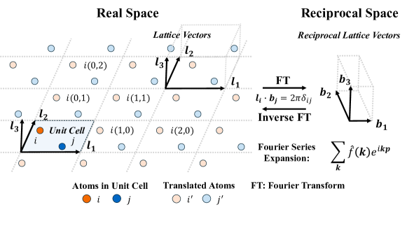
Figure 1: Illustration of the relationship between real space (left) and reciprocal space (right) in crystals. Long-range interactions can be commutated through Fourier series expansion. More details can be found in Section˜2.2.

2.1 Periodic Crystal Structure Representation

A crystalline material can be represented as the infinite periodic arrangement of atoms in 3D space, with the smallest repeating structural unit referred to as the unit cell. The unit cell defines the lattice symmetry and dictates the overall periodicity and physical properties of the material. The structure of crystals is commonly represented using two coordinate systems: the Cartesian coordinate system and the fractional coordinate system.

Cartesian coordinate.

Mathematically, a material can be represented as $\mathbf{M}=(\mathbf{A},\mathbf{P},\mathbf{L})$. $\mathbf{A}=[\bm{a}_{1},\bm{a}_{2},\cdots,\bm{a}_{n}]^{\top}\in\mathbb{R}^{n\times h}$ denotes the atom feature matrix for $n$ atoms within a unit cell, where $\bm{a}_{i}\in\mathbb{R}^{h}$ represents the $h$-dimensional features of atom $i$ in the unit cell. $\textbf{P}=[\bm{p}_{1},\bm{p}_{2},\cdots,\bm{p}_{n}]^{\top}\in\mathbb{R}^{n\times 3}$ is the position matrix, where $\bm{p}_{i}\in\mathbb{R}^{3}$ is the Cartesian coordinate of atom $i$ inside the unit cell. In crystallography, a lattice is a periodic arrangement of points that defines a crystal’s translational symmetry. As shown in Figure˜1, the lattice matrix $\textbf{L}=[\bm{\ell}_{1},\bm{\ell}_{2},\bm{\ell}_{3}]^{\top}\in\mathbb{R}^{3\times 3}$ consists of three translation lattice vectors that determine the shape and periodicity of the unit cell. The periodic repetition of the unit cell is described by integer multiples of the lattice vectors, ensuring translational invariance. Specifically, the infinite crystal structure can be expressed as:

$$\hat{\mathbf{P}}=\{ \hat{\bm{p}_{i}}|\hat{\bm{p}_{i}}=\bm{p}_{i}+n_{1}\bm{\ell}_{1}+n_{2}\bm{\ell}_{2}+n_{3}\bm{\ell}_{3},$$

$$n_{1},n_{2},n_{3}\in\mathbb{Z},i\in\mathbb{Z},1\leq i\leq n\}$$

where the integers $n_{1},n_{2},n_{3}$ define a 3D translation with $\bm{\ell}_{1},\bm{\ell}_{2},\bm{\ell}_{3}$. $\hat{\mathbf{A}}=\{\hat{\bm{a}_{i}}|\hat{\bm{a}_{i}}=\bm{a}_{i},i\in\mathbb{Z},1\leq i\leq n\}$ is the atom feature in repeated unit cells, which remains unchanged under periodic translation.

Fractional coordinate.

Fractional coordinates capture the relative positions of atoms within the unit cell and offer significant advantages for periodic materials compared to Cartesian coordinates. Specifically, the fractional coordinate uses the lattice matrix $\textbf{L}\in\mathbb{R}^{3\times 3}$ as the basis, where atomic positions are described by fractional coordinate vectors $\bm{f_{i}}=[f_{1},f_{2},f_{3}]^{\top}\in[0,1)^{3}$. The corresponding Cartesian coordinates are obtained as $\bm{p}_{i}=\bm{L}\bm{f_{i}}$, where $\bm{p}_{i}=f_{1}\bm{\ell}_{1}+f_{2}\bm{\ell}_{2}+f_{3}\bm{\ell}_{3}$. The representation of crystal $\mathbf{M}$ generalizes to $\mathbf{M}=(\mathbf{A},\mathbf{F},\mathbf{L})$, where $\mathbf{F}=[\bm{f}_{1},\cdots,\bm{f}_{n}]^{\top}\in[0,1)^{n\times 3}$ denotes the fractional coordinates of all atoms in the unit cell. Fractional coordinates inherently align with lattice periodicity, ensuring that calculations respect periodic boundary conditions. Moreover, they remain invariant under space group operations, such as translations and rotations, thereby preserving structural relationships. These properties make fractional coordinates a more efficient and symmetry-aware representation for periodic materials compared to Cartesian coordinates.

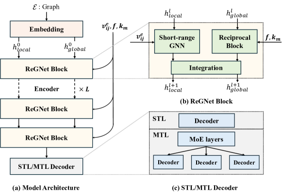
Figure 2: Overall framework architecture and details of each block, consisting of three main components: (a) Model architecture, (b) ReGNet block, and (c) STL/MTL Decoder. The Model Architecture utilizes multiple ReGNet blocks. Each ReGNet block (b) combines local features through graph message passing and global features via reciprocal space convolution to update node embeddings. The STL/MTL Decoder (c) outputs material property predictions, supporting both single-task (STL) and multi-task (MTL) learning setups.

2.2 Reciprocal Space in Crystalline Materials

Reciprocal space is essential for understanding important natures of materials such as electronic, structural, and vibrational properties (Ashcroft & Mermin, 2001; Gross & Marx, 2014). Integrating its representations can enhance predictive accuracy by capturing global periodicity and long-range interactions. Reciprocal space consists of wave vectors $\bm{k}$ spanned by reciprocal lattice vectors $\bm{b_{1}},\bm{b_{2}},\bm{b_{3}}$, which are derived from lattice vectors in real space $\bm{\ell}_{1},\bm{\ell}_{2},\bm{\ell}_{3}$. Each vector in reciprocal space represents a spatial frequency that encodes crystal periodicity along specific directions. More details can be found in Appendix˜A.

To establish the reciprocal space representation, we employ the Fourier transform, which expresses periodic function $f$ via Fourier series expansion:

$$f(\bm{p}_{j})=\sum_{\bm{k}}\hat{f}(\bm{k})\exp(i\bm{k}\cdot\bm{p}_{j}),$$ (1)

where $\hat{f}(\bm{k})$ represents the Fourier coefficients, encoding the contributions of wave vectors $\bm{k}$ at atom $j$. The corresponding inverse transform, which computes $\hat{f}(\bm{k})$ from the real-space representation $f(\bm{p}_{j})$, is given by:

$$\hat{f}(\bm{k})=\frac{1}{\Omega}\sum_{j\in S}h_{j}\exp(-i\bm{k}\cdot\bm{p}_{j}),$$ (2)

where $S$ denotes the set of atomic positions in the crystal lattice, $h_{j}$ represents function values at site $\bm{p}_{j}$ such as nuclear embedding, and $\Omega$ is the system volume.

2.3 MTL and MoE

Multi-Task Learning (MTL) typically employs a shared backbone network to extract common features, followed by task-specific output heads (decoders) that specialize in individual predictions (Xiao et al., 2024). In this context, the Mixture of Experts (MoE) framework offers a flexible and scalable approach to capture both shared and task-specific features by leveraging task-relevant experts. MoE has gained significant attention in multi-task scenarios across computer vision and natural language processing due to its adaptability and efficiency (Riquelme et al., 2021). An MoE layer consists of a set of expert networks, denoted as $E_{i},\forall i\in[1,N]$, where $N$ is the number of experts along with a routing network $R$. The output of an MoE layer is the weighted sum of the output $E_{n}(x)$ from every expert, where weights $G_{n}(x)$ are calculated by the routing network $R$ and $x$ represent the model input. Formally, the output of a MoE layer is given by

$$y=\sum_{i=1}^{N}G_{n}(x)E_{n}(x).$$

The routing network utilizes a noisy Top-$K$ selection mechanism (Shazeer et al., 2017) to model the probabilities of each expert and select the top $K$ candidates. This process is defined as:

$$G(x)=\text{TopK}(\text{Softmax}(xW+\mathcal{N}(0,1)\text{Softplus}(xW_{\text{noise}}))),$$

where $W$ and $W_{\text{noise}}$ are router model parameters, $\mathcal{N}(0,1)$ is a standard normal distribution, and Softmax($\cdot$) and Softplus($\cdot$) are activation functions. Besides, the TopK($\cdot$) function retains only the $K$ largest values, setting all others to zero.

3 Method

This work focuses on predicting the thermodynamic, electronic, and mechanical properties of crystalline materials through a novel approach that explicitly incorporates long-range interactions from reciprocal space. The architectures of ReGNet and its multi-task variant, ReGNet-MT, are illustrated in Figure˜2. Unlike Lin et al. (2023) which employs fixed physical potentials as physics-informed edge features, our approach employs continuous filters with Fourier transforms, utilizing learnable parameters to encode reciprocal space representations while preserving the periodic symmetry of crystalline systems. Inspired by the molecular graph framework in Kosmala et al. (2023), we propose the ReciprocalBlock, a specialized module designed to capture long-range interaction in crystalline materials. This module leverages reciprocal lattice vectors and atomic fractional coordinates, eliminating reliance on predefined supercell grid sizes. Therefore, our approach enhances symmetry and periodicity preservation in long-range representations. Besides, we incorporate GNN with our ReciprocalBlock to model short- and long-range information in materials. Lastly, we enable multi-property prediction by leveraging MoE.

3.1 Representation and Embedding

Invariant crystal graph and embedding.

Firstly, we construct a radius-based graph, where nodes represent atoms and edges encode atomic interactions within a predefined cutoff radius $r_{\text{cut}}$. Formally, the edge set is defined as:

$$\mathcal{E}=\{e_{ij}:\|\bm{p}_{i}-\bm{p}_{j}\|_{2}\leq r_{\text{cut}},\ \forall i,j\in V\},$$

where $V$ is the set of nodes, and distances between nodes are computed based on their 3D Cartesian coordinates $\bm{p}_{i}$ and $\bm{p}_{j}$.

Once the crystal graph is established, we can proceed to obtain embeddings for nodes and edges. Node feature $\bm{a}_{i}$ for node $i$ is first mapped using CGCNN (Xie & Grossman, 2018) embeddings, followed by a linear transformation to initialize the short-range node features $h_{i,\text{local}}^{0}$. The initial global atom representation is derived through a linear transformation of ${h}^{0}_{\text{local}}$, as shown below:

$$h^{0}_{\text{global}}=\sigma(W_{r}h^{0}_{\text{local}}),$$

where $W_{r}$ is a learnable weight matrix. We use ${h}^{0}_{\text{global}}$ as initial long-range node features. The invariant edge feature $||\mathbf{p}_{i}-\mathbf{p}_{j}||_{2}$ is defined by the Euclidean distance between node pair $i$ and $j$, are scaled by $c/||\mathbf{p}_{i}-\mathbf{p}_{j}||_{2}$, where c is a chosen constant to mimic the pairwise potential in Lin et al. (2023). These values are then embedded using radial basis function (RBF) kernels to get the initial edge features ${v}_{ij}^{e}$. More details are shown in Section˜B.2

Fractional coordinates and reciprocal lattice vectors.

To effectively extract features from long-range information in reciprocal space, we propose using fractional coordinates $\bm{f}$ and basis reciprocal lattice vectors $\bm{k}_{m}$ with continuous filters convolution. Together, they enable a precise and symmetry-consistent representation of periodic structures (discussed in Section˜2). Our approach differs from previous methods (Kosmala et al., 2023) for the following reasons. First, for crystalline materials, Cartesian coordinates can introduce ambiguities, as identical crystal structures may be expressed differently due to periodic transformations, such as translations or rotations. For example, the lattice matrices $\textbf{L}=[\bm{\ell}_{1},\bm{\ell}_{2},\bm{\ell}_{3}]^{\top}$ and $\textbf{L}^{\prime}=[\bm{\ell}_{1}+\bm{\ell}_{2},\bm{\ell}_{2},\bm{\ell}_{3}]^{\top}$ describe identical periodic patterns but differ in their Cartesian representations. In contrast, fractional coordinates normalize atomic positions relative to the unit cell, ensuring invariance under periodic transformations and eliminating redundancies in Cartesian representations. Second, it relies on a predefined grid size as hyperparameters to cover all relevant frequencies as $\bm{k}$, which could disrupt the unit cell symmetry and substantially increase computational costs, particularly for large unit cells and complex systems. Instead, our method leverages the natural periodicity of the lattice in materials, avoiding redundant grid parameterization and ensuring a symmetry-consistent representation of long-range interactions. Therefore, by combining fractional coordinates $\bm{f}$ and basis reciprocal lattice vectors $\bm{k}_{m}$, we achieve an effective framework for feature extraction in reciprocal space, accurately capturing the long-range information of crystal materials.

With the aforementioned representations, our model enables both short-range and long-range message passing to effectively capture comprehensive material structural features.

3.2 Short-Range Message Passing

We employ the short-range block in Figure˜2(b) to update the atomic representations using an invariant graph neural network with multiple message-passing layers. Each node aggregates information only from its geometric neighbors within the cutoff radius $r_{\text{cut}}$. Therefore, we naturally interpret this as capturing the short-range information to material representations. The computational process at the $\ell$-th message-passing layer for a node $i$ is expressed as:

$$h_{i,\text{local}}^{\ell+1}\leftarrow g\left(h_{i,\text{local}}^{\ell},\sum_{j\in V}\phi\left(h_{i,\text{local}}^{\ell},h_{j,\text{local}}^{\ell},v_{ij}^{e}\right)\right),$$ (3)

where $h_{i,\text{local}}^{\ell}$ represents the embedding features of node $i$ at the $\ell$-th layer. Here, $g$ and $\phi$ are trainable layers within the GNN. Specifically, $\phi$ computes interactions between node embeddings and edge features $v_{ij}^{e}$, while $g$ aggregates these messages to update the node embeddings. Further details on the architecture of the local geometric GNN are provided in Appendix B.

3.3 Long-Range Message Passing

To complement the short-range modeling, we employ the long-range block in Figure˜2(b) to globally update the atomic representations using the ReciprocalBlock. Specifically, this block leverages Fourier transform-based continuous filters with neural networks to encode periodic structures from reciprocal space. Besides, as discussed in Section˜3.1, we utilize atomic fractional coordinates $\bm{f}$ and basis reciprocal lattice vectors $\bm{k}_{m}$ to extract structural information from reciprocal space and update the node features in the model block. The global embeddings are computed iteratively:

$$h^{\ell+1}_{\text{global}}=\text{ReciprocalBlock}({h}_{\text{global}}^{\ell},\bm{f},\bm{k}_{m}),$$

where ${h}^{\ell}_{\text{global}}$ represents the input embeddings from the $\ell$-th layer.

Reciprocal block.

Here, we explain the reciprocal block in detail. The reciprocal block incorporates long-range interactions into the node embeddings using continuous filters on features derived from Fourier transforms. Each material $m$ has reciprocal lattice vectors $\bm{k}_{m}$ based on the lattice vector in real space. The set of atoms in the material is denoted as $\mathcal{I}_{m}$, where $j\in\mathcal{I}_{m}$ represents all atoms within material $m$. This block aggregates the contributions of all atoms in each material to compute a global representation in the reciprocal domain. For each material $m$, the reciprocal embedding ${r}_{{}_{m}}$ is computed as:

$${r}_{m}=\sum_{j\in\mathcal{I}_{m}}{h}_{j,\text{global}}^{\ell}\cdot\exp(-i\bm{k}_{m}^{\top}\bm{f}_{j}),$$

where ${h}_{j,\text{global}}^{\ell}$ is the global embedding of atom $j$ from $\ell$-th layer, $\bm{f}_{j}$ is its fractional coordinate, and $i$ is the imaginary unit. This operation aggregates atomic embeddings into a single reciprocal representation for materials, capturing global periodic interactions.

Subsequently, the reciprocal embedding ${r}_{m}$ undergoes an inverse Fourier transform to be mapped back into real space for the atoms in material $m$. This process can be expressed as below:

$$\tilde{h}_{\text{global}}^{\ell}=\sum_{j\in\mathcal{I}_{m}}\exp(i\bm{k}_{m}^{\top}\bm{f}_{j})\cdot{r}_{m}\cdot\mathbf{W}_{\text{filter}},$$

where $\exp(i\bm{k}_{m}^{\top}\bm{f}_{j})$ performs the inverse Fourier transform to map the reciprocal representation back to the real domain. $\mathbf{W}_{\text{filter}}$ is a trainable filter refining the reciprocal embedding, selectively emphasizing important contributions from the reciprocal space features to model long-range interactions. In addition, the prefactor $\frac{1}{\Omega}$ in eq.˜2 is incorporated into the learned filter $\mathbf{W}_{\text{filter}}$, without requiring explicit normalization by the system volume. In a word, this operation effectively incorporates long-range interactions and periodicity from the reciprocal domain into the real-space representation of each atom $j\in\mathcal{I}_{m}$.

Finally, the global embeddings $\tilde{{h}}^{\ell}_{\text{global}}$ are updated using residual connections to get ${h}^{\ell+1}_{\text{global}}$, as shown below.

$${h}^{\ell+1}_{\text{global}}={h}^{\ell}_{\text{global}}+\tilde{{h}}^{\ell}_{\text{global}}.$$

At this point, the complete process of a Reciprocal Block has been fully described.

3.4 Hierarchical Embedding Integration

Our model employs multiple ReGNet blocks to integrate local and global information at each layer. Within each block, node embeddings are updated by combining contributions from short-range graph message passing and long-range reciprocal-based message passing. The resulting integrated embeddings are passed to the next block, enabling the model to propagate and refine hierarchical representations of material structures. This approach ensures the effective capture of both local atomic-scale features and global lattice-scale features throughout the network.

3.5 Decoder Block

Single-property prediction.

After completing the iterative message-passing steps, node features are aggregated within each graph using mean pooling, which captures the overall structural information of the material. The resulting graph-level representation is then processed through fully connected layers to predict the target material property.

Multi-property prediction.

When doing multi-property prediction, we employ an MTL decoder, consisting of MoE layers and task-specific heads (fully connected layers in our case). We assume that the aggregated node features from the final ReGNet block encapsulate both short-range and long-range information of materials, that can be shared among all property prediction tasks. However, different properties require customized features before individual task heads. Therefore, experts are expected to learn distinct features, while the routing network can determine the optimal expert combination. Unlike the post-processing of the predicted property values after decoders with physical laws (Ren et al., 2024), this approach offers more flexibility. Meanwhile, similar properties could have a large expert selection overlap such that the knowledge can be shared among them. Notably, this expert-sharing mechanism facilitates positive transfer.

Table 1: Comparison of test MAE on The Materials Project dataset. The best results are highlighted in bold, while the second-best results are indicated with underlines. The symbol $\bm{|}$ separates results from two distinct 2-property prediction experiments, where the four properties are divided into two groups and trained separately.

	Formation Energy	Band Gap	Bulk Moduli	Shear Moduli
Method	meV/atom	eV	log(GPa)	log(GPa)
CGCNN	31	0.292	0.047	0.077
SchNet	33	0.345	0.066	0.099
MEGNET	30	0.307	0.060	0.099
GATGNN	33	0.280	0.045	0.075
ALIGNN	22	0.218	0.051	0.078
Matformer	21.0	0.211	0.043	0.073
PotNet	18.8	0.204	0.040	0.0650
Crystalformer	18.6	0.198	0.0377	0.0689
eComFormer	18.16	0.202	0.0417	0.0729
iComFormer	18.26	0.193	0.0380	0.0637
ReGNet	17.07	0.189	0.0328	0.0628
ReGNet-MT	24.50	0.218	0.0391	0.0668

4 Related Work

Crystal property prediction.

Crystal property prediction has been widely studied using both physics-based and deep-learning approaches. Traditional physics-based methods, such as Coulomb matrices (Rupp et al., 2012; Elton et al., 2018), effectively model ionic and metallic materials but lack generalization due to constraints like permutation invariance. Deep learning has introduced more flexible predictions by representing crystals as chemical formulas and using sequence models (Jha et al., 2018; Goodall & Lee, 2020; Wang et al., 2021). More recent methods leverage 3D geometric structures, modeling crystals as 3D graphs with graph neural networks (GNNs) (Schütt et al., 2017; Gasteiger et al., 2020). Key advances include CGCNN (Xie & Grossman, 2018), which utilized multi-edge graphs to model periodic invariance, inspiring methods such as ALIGNN (Choudhary & DeCost, 2021), which incorporated angle-based features, and Matformer (Yan et al., 2022), which captured periodic patterns using self-connecting edges. PotNet (Lin et al., 2023) proposed physics-informed edge features that embed the infinite summation of pre-defined interatomic potentials, while Crystalformer (Taniai et al., 2024) encoded periodic structures with infinitely connected attention. Yan et al. (2024) introduced iComFormer with invariant descriptors and eComFormer with equivariant vectors. Despite significant advancements, many approaches still face limitations in accurately capturing periodic patterns and long-range interactions while maintaining computational efficiency and reliable generalization.

Long-range interaction modeling.

Modeling long-range interactions remains a significant challenge. Early approaches augmented physical equations with hand-crafted terms (Staacke et al., 2021) or predicted atomic charges (Unke et al., 2021), while recent methods focus on data-driven learning. Yu et al. (2022) computed scalar-valued structure factors and integrates them with GNN outputs only in the final layer, limiting interaction between reciprocal space and local features. In contrast, Kosmala et al. (2023) integrated structure factor embeddings directly into GNN message passing, enabling feedback to node embeddings. However, it requires extensive hyperparameter tuning for grid sizes ($N_{x},N_{y},N_{z}$) to define the supercell, which can disrupt the symmetry of the unit cell, alter its space group, and substantially increase computational costs, particularly for systems with complex symmetries. Lin et al. (2023) considered the infinite summations of pairwise atomic interactions with additional computational cost $\mathcal{O}(n^{2})$, relied on precomputed, non-trainable physical potentials as edge features, which limited adaptability to diverse material systems and further increased computational overhead.

Multi-property prediction.

While multi-property prediction in materials remains largely unexplored, we summarize several advances in molecular domains. Liu et al. (2022) introduced the MTL concept in molecular property prediction in the early stage. Their approach involves constructing a sparse dataset and relying on prior knowledge of property relations before training. Christofidellis et al. (2023) proposed a language model that bridges natural and chemical languages to perform multi-task learning, such as chemical reaction prediction and retrosynthesis. However, their work is not specifically focused on multi-property prediction. Additionally, Beaini et al. (2023) developed a foundation model and a large-scale molecular dataset tailored for multi-task learning. Nevertheless, there is currently no comparably large material dataset to support a similar effort. In another approach, Ren et al. (2024) leveraged physical laws after task decoders to address data heterogeneity across different properties, improving prediction consistency. In contrast, we integrate the Mixture of Experts (MoE) between encoders and decoders, allowing each task to obtain customized structural features before property prediction.

5 Experimental Studies

Table 2: Comparison of test MAE on the JARVIS dataset. The best results are highlighted in bold, and the second-best results are indicated with underlines. Lower test MAE indicates better results.

	Form. Energy	Bandgap(OPT)	$E_{\text{total}}$	Bandgap(MBJ)	$E_{\text{hull}}$
Method	meV/atom	eV	meV/atom	eV	meV
CGCNN	63	0.20	78	0.41	170
SchNet	45	0.19	47	0.43	140
MEGNET	47	0.145	58	0.34	84
GATGNN	47	0.170	56	0.51	120
ALIGNN	33.1	0.142	37	0.31	76
Matformer	32.5	0.137	35	0.30	64
PotNet	29.4	0.127	32	0.27	55
Crystalformer	30.6	0.128	32	0.27	46
eComFormer	28.4	0.124	32	0.28	44
iComFormer	27.2	0.122	28.8	0.26	47
ReGNet	27.0	0.127	26.8	0.24	48
ReGNet-MT	35.0	0.122	36.0	0.21	69.2

5.1 Experimental Setup

We conduct a series of experiments using two widely recognized datasets in materials science. Materials Project (Chen et al., 2019) is a collection of 69239 crystals from the Materials Project database retrieved by Chen et al. (2019), with regression tasks of formation energy, bandgap, bulk modulus, and shear modulus. JARVIS-DFT (Choudhary et al., 2020) is a collection of 55723 crystals, with regression tasks of formation energy, total energy, bandgap (OPT), bandgap (MBJ), and energy above hull ($E_{\text{hull}}$). These datasets cover a range of scales, including 69239 crystals for large-scale tasks, 18171 crystals for medium-scale tasks, and 5450 crystals for small-scale tasks.

To ensure consistency, we adopt experimental settings aligned with prior works, including MatFormer (Yan et al., 2022) and PotNet (Lin et al., 2023). We benchmark against several baseline methods, including CGCNN (Xie & Grossman, 2018), SchNet (Schütt et al., 2017), MEGNet (Chen et al., 2019), GATGNN (Louis et al., 2020), ALIGNN (Choudhary & DeCost, 2021), MatFormer (Yan et al., 2022), PotNet (Lin et al., 2023), Crystalformer (Taniai et al., 2024), and ComFormer (Yan et al., 2024). All experiments are conducted on NVIDIA A100 GPUs. Additional details on the experimental configurations and ReGNet’s settings are provided in Appendix B.

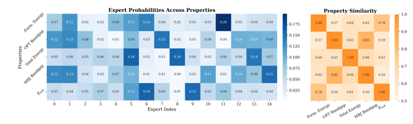
Figure 3: MoE experts frequencies for each property on the JARVIS dataset and property similarities. The expert selections in OPT bandgap and MBJ bandgap show the highest similarity and positive transfer happens between these two predictions.

5.2 Experimental Results

ReGNet achieves state-of-the-art performance across various crystal property prediction tasks. On the Materials Project dataset, ReGNet consistently outperforms previous works across all four tasks, achieving the best results with significant margins as shown in Table˜1. For predicting two energy properties and two mechanical properties, we apply two ReGNet-MT models separately, achieving comparable performance. For the JARVIS dataset, as shown in Table˜2, ReGNet surpasses baseline models in three out of five tasks: formation energy, $E_{\text{total}}$, and band gap (MBJ), while achieving competitive results on $E_{\text{hull}}$ and band gap (OPT). Notably, it consistently outperforms PotNet across all tasks. ReGNet-MT on all 5-property prediction delivers the best results for band gap (OPT) and band gap (MBJ), outperforming all single-property prediction models, while maintaining comparable performance on the remaining tasks.

The superior performance of ReGNet and ReGNet-MT is attributed to several key factors. ReGNet leverages trainable Fourier filters from reciprocal space to capture long-range interactions while preserving the periodic symmetry of crystal structures. In contrast, prior methods rely on fixed physical potentials or predefined grid sizes that require tuning. Besides, by integrating reciprocal-space-based global information with GNN-driven local modeling, ReGNet provides a comprehensive representation of crystalline materials. Additionally, ReGNet-MT benefits from positive task transfer, achieving superior performance on band gap (OPT) and band gap (MBJ) in the 5-property prediction.

Table 3: Ablation studies for the effects of reciprocal space and number of blocks.

Method	JARVIS Formation Energy
	meV/atom
ReGNet w/o Reciprocal(3)	29.6
ReGNet(3)	27.8
ReGNet(4)	27.0

5.3 Model Efficiency Comparison

As shown in Table˜4, we evaluate the computational efficiency of ReGNet and ReGNet-MT by comparing their model parameters and training time per epoch with ALIGNN, Matformer, PotNet, and ComFormer on the JARVIS formation energy task. We use 3 and 4 to indicate the number of blocks in ReGNet, which covers all experimental settings of ReGNet. ReGNet demonstrates superior computational efficiency, with ReGNet(3) achieving the fastest training time per epoch among all models. Notably, in the multi-task setting, ReGNet-MT predicts five properties simultaneously. The training time does not even double that of single-task ReGNet, and the model’s parameter size is smaller than that of single-task eComFormer. It is also important to note that PotNet reduces its training time by precomputing infinite potential summations for the training data, which is not employed in ReGNet. This highlights the efficiency of ReGNet in handling both single-task and multi-task scenarios.

Table 4: Comparison of model efficiency on JARVIS formation energy prediction. We include training time per epoch, 1-task model parameter size, and 5-task model parameter size. N/A denotes that ReGNet-MT is not designed for single-property prediction.

Method	Time/Epoch	1-task Model Para.	5-task Model Para.
ALIGNN	261 s	4.0 M	20.0 M
Matformer	51 s	2.9 M	14.5 M
PotNet	34 s	1.8 M	9.0 M
iComFormer	62 s	5.0 M	25.0 M
eComFormer	92 s	12.4 M	62.0 M
ReGNet(3)	31 s	3.3 M	16.5 M
ReGNet(4)	38 s	4.3 M	21.5 M
ReGNet-MT	60 s	N/A	9.5 M

5.4 Ablation Studies

In this section, we highlight the significance of incorporating reciprocal space information and analyze the impact of the number of ReGNet blocks. As shown in Table˜3, the inclusion of reciprocal space information enhances performance. Additionally, increasing the number of ReGNet blocks further improves performance. However, to balance accuracy and computational efficiency, we limit the maximum number of blocks to 4 in all results, as additional blocks introduce higher computational overhead. Detailed results of the ablation study on the JARVIS dataset are presented in Table˜9 within Section˜B.5.

5.5 Understanding ReGNet-MT

In the experimental evaluation of ReGNet-MT on the JARVIS dataset for jointly predicting five properties, the model achieves the best performance for two bandgaps due to positive transfer though some degradation happens. Notably, bandgap (MBJ) surpasses the state-of-the-art (SOTA) results of single-task models, while bandgap (OPT) matches the SOTA performance. To evaluate this improvement, we track the selection frequencies of the 15 experts and visualize the expert selection probabilities for each task (see Figure˜3, left). We also compute the cosine similarity among properties via expert selection probabilities (see Figure˜3, right). Among the five tasks, the two bandgap properties exhibit the highest similarity score of 0.85, indicating a big overlap in the expert selection, which facilitates the positive transfer. This finding explains why ReGNet-MT outperforms single-task training for two bandgaps.

6 Limitation

One limitation of our study lies in using geometric GNNs for short-range modeling to capture local features. While effective, recent advancements in Transformer-based models (Yan et al., 2022, 2024) present opportunities for further improvement by incorporating reciprocal space information to enhance the structural representation of materials. Besides, multi-property prediction remains an area worthy of further exploration, as current efficient multi-task learning methods can be explored. Despite these limitations, our study provides a new perspective on modeling crystal materials by leveraging reciprocal-space-based long-range information alongside graph-based short-range information.

7 Conclusion

In this paper, we introduce a novel model, ReGNet, designed to capture the reciprocal space-based long-range information and geometric GNNs short-range information, in crystal property prediction. Besides, its multi-task variant, ReGNet-MT with the help of MoE, explores the multi-property prediction. Empirically, ReGNet achieves significant performance improvement on prevalent benchmarks and ReGNet-MT achieves the best results in 2 bandgap properties efficiently. We hope that this efficient model provides a valuable perspective in terms of both ML and materials science to promote further interdisciplinary research and encourage its applications in various materials systems.

Appendix A Reciprocal Space Concepts

A.1 Relations Between Real and Reciprocal Lattice Vectors

In materials science, crystals exhibit translational symmetry, where atoms are periodically arranged in 3D space, forming a direct lattice in real space. Each lattice point corresponds to a repeating unit in the crystal structure, described by primitive lattice vectors $\bm{\ell}_{1},\bm{\ell}_{2},\bm{\ell}_{3}$. Reciprocal space, on the other hand, represents the spatial frequencies associated with this periodic arrangement. It forms a dual lattice, mathematically related to the real lattice through reciprocal lattice vectors $\bm{b}_{1},\bm{b}_{2},\bm{b}_{3}$. $V$ is the volume of the parallelepiped spanned by the three primitive translation vectors of the original Bravais lattice. It remains invariant under periodic permutations of the indices (Economou, 2010).

Volume and vectors are defined as:

$$V ={\bm{\ell}_{1}\cdot(\bm{\ell}_{2}\times\bm{\ell}_{3})}$$ (4)

$$\bm{b}_{1} =2\pi\cdot\frac{\bm{\ell}_{2}\times\bm{\ell}_{3}}{V}$$ (5)

$$\bm{b}_{2} =2\pi\cdot\frac{\bm{\ell}_{3}\times\bm{\ell}_{1}}{V}$$ (6)

$$\bm{b}_{3} =2\pi\cdot\frac{\bm{\ell}_{1}\times\bm{\ell}_{2}}{V}$$ (7)

These vectors satisfy the reciprocal relationship:

$$\bm{\ell}_{i}\cdot\bm{b}_{j}=2\pi\delta_{ij}.$$ (8)

The symbol $\delta_{ij}$ represents Kronecker delta, which is a mathematical function defined as:

$$\delta_{ij}=\begin{cases}1,&\text{if }i=j\\ 0,&\text{if }i\neq j\end{cases}$$ (9)

This allows us to define a periodic function naturally in reciprocal space, where vectors $\bm{k}\in\Lambda$ can be expanded in terms of these reciprocal basis vectors (Ashcroft & Mermin, 2001).

The 3D spatial frequencies must be integer combinations of three spatial basis frequencies $\bm{b}_{1},\bm{b}_{2},\bm{b}_{3}\in\mathbb{R}^{3\times 3}$ spanning the reciprocal lattice:

$$\Lambda=\{n_{1}^{\prime}\bm{b}_{1}+n_{2}^{\prime}\bm{b}_{2}+n_{3}^{\prime}\bm{b}_{3}|n_{1}^{\prime},n_{2}^{\prime},n_{3}^{\prime}\in\mathbb{Z}\}.$$ (10)

A.2 Diffraction Methods

Reciprocal space is fundamental to diffraction techniques such as X-ray diffraction (XRD) and electron diffraction. XRD is a widely used technique in crystallography that examines the constructive interference of X-rays scattered by periodic atomic planes, providing detailed insights into crystal structures (Ladd et al., 1977). Similarly, in electron diffraction, the elastic scattering of electrons by atoms produces diffraction patterns that reveal structural information (Egerton et al., 2005). The scattering intensity is modeled using the structure factor:

$$S(\mathbf{G})=\sum_{j}f_{j}e^{-i\mathbf{G}\cdot\mathbf{r}_{j}}$$ (11)

where $\mathbf{G}$ is the reciprocal lattice vector. $f_{j}$ represents the atomic form factor in X-ray diffraction, and the electron scattering factor in electron diffraction separately. Diffraction patterns are governed by Bragg’s law:

$$n\lambda=2d\sin\theta,$$ (12)

relating lattice spacings ($d$) to diffraction angles ($\theta$) and wavelength ($\lambda$) (Cullity & Smoluchowski, 1957). Notably, this condition applies to both XRD and ED, although electron diffraction often requires consideration of dynamical scattering effects due to stronger interactions between electrons and matter (James, 1963).

Electron diffraction is widely used in transmission electron microscopy (TEM) to analyze materials. For instance, single crystals produce discrete spot patterns, polycrystals form concentric rings, and amorphous materials show diffuse rings (Egerton et al., 2005). These patterns enable crystallinity and orientation analysis, with applications in semiconductors, metals, and oxides. Figure˜4 illustrates a typical diffraction pattern. By satisfying the Bragg condition, elastically scattered electrons produce high-intensity spots, with the angular relationship between transmitted and diffracted beams revealing the crystal structure (Poeppelmeier, 2023).

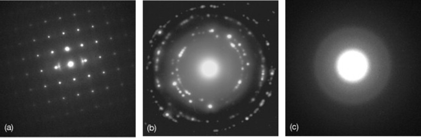
Figure 4: Example of electron diffraction patterns from Poeppelmeier (2023).

A.3 Electronic Band

Reciprocal space plays a crucial role in determining electronic and vibrational properties. Specifically, Bloch’s theorem relates the electron wavefunction $\psi(\mathbf{r})$ to the wave vector $\bm{k}$ as:

$$\psi(\mathbf{r})=e^{i\bm{k}\cdot\mathbf{r}}u(\mathbf{r})$$ (13)

where $\psi(\mathbf{r})$ is the electronic wavefunction, $\bm{k}$ is the wave vector in reciprocal space. This theorem facilitates the study of electronic band structures, enabling the prediction of properties like band gaps and carrier mobility (Ashcroft et al., 1978).

$u(\mathbf{r})$ is a function periodic with the lattice, and r denotes position:

$$u(\mathbf{r}+\mathbf{R})=u(\mathbf{r})$$ (14)

with $\mathbf{R}$ being a lattice translation vector. This decomposition separates the plane wave component, representing long-range propagation, and the periodic modulation, capturing local interactions within the unit cell.

The energy eigenvalues, plotted as a function of $\bm{k}$ within the first Brillouin zone (Ashcroft & Mermin, 2001), form a band structure that determines key material properties, including band gaps which distinguish insulators, semiconductors, and metals, effective mass and carrier mobility which influence electronic conductivity, and optical absorption spectra and dielectric constants which govern photon-electron interactions and optoelectronic performance (Ziman, 2001).

Appendix B Experimental Details

B.1 Dataset

We provide more details for the JARVIS and Materials Project datasets in this section.

Table 5: Dataset sizes vary for different properties.

Dataset	Task	Total
JARVIS-DFT	Formation Energy	55722
	Bandgap (OPT)	55722
	Total Energy	55722
	Bandgap (MBJ)	18171
	$E_{\text{hull}}$	55370
Materials Project	Formation Energy	69239
	Band Gap	69239
	Bulk Moduli	5450
	Shear Moduli	5450

The Materials Project Dataset

The Materials Project dataset, introduced by Chen et al. (2019), is a comprehensive collection of 69239 materials, widely utilized in crystal property prediction studies. We adopt the data splits in Yan et al. (2024) to ensure consistency and fair comparisons with prior methods. Specifically, for formation energy and bandgap prediction tasks, the dataset comprises 60000, 5000, and 4239 crystals for training, validation, and testing, respectively. For bulk modulus and shear modulus predictions, the splits include 4664, 393, and 393 crystals. Notably, one validation sample in the shear modulus task is excluded due to a negative GPa value, reflecting an underlying unstable or metastable crystal structure. Among the included crystals, 30084 have been experimentally observed, further highlighting the dataset’s reliability for studying material properties.

The JARVIS Dataset

The JARVIS dataset, proposed by Choudhary et al. (2020), contains 55723 materials and serves as a benchmark for crystal property prediction. Following the experimental protocols of Yan et al. (2024), we evaluate our methods on five regression tasks: formation energy, total energy, bandgap (using both OPT and MBJ methods), and energy above the convex hull (Ehull). The training, validation, and testing splits for formation energy, total energy, and OPT bandgap consist of 44578, 5572, and 5572 crystals, respectively. The splits for Ehull include 44296, 5537, and 5537 crystals, while MBJ bandgap tasks consist of 14537, 1817, and 1817 crystals. The MBJ functional is considered more accurate for bandgap calculations compared to OPT, and both are utilized in this study. Notably, 18865 of the dataset’s crystal structures have been experimentally observed, adding robustness to its use in predictive modeling.

B.2 Settings of Model Embeddings

Node feature is embedded into a CGCNN (Xie & Grossman, 2018) embedding vector of length 92 based on atomic number, and then mapped to a 256-dimensional initial short-range node feature ${h}^{0}_{\text{local}}$ by a linear transformation. The initial global node feature ${h}^{0}_{\text{global}}$ is obtained by linear transformation on ${h}^{0}_{\text{local}}$ and follows an activation function. The invariant edge feature $||\mathbf{p}_{i}-\mathbf{p}_{j}||_{2}$ is inversely scaled to $-0.75/||\mathbf{p}_{i}-\mathbf{p}_{j}||_{2}$ based on Lin et al. (2023), and then expanded into a 256-dimensional vector by RBF kernels with 256 center values from -4.0 to 4.0; after that, we transfer the 256-dimensional vector to initial edge feature ${v}_{ij}^{e}$ through a linear transformation followed by a SoftPlus activation.

B.3 Geometric GNN Information

Building on PotNet (Lin et al., 2023), we adopt its base model as the local graph component, without using its additional computed infinite summation of interatomic potentials. The local module performs iterative message passing over the constructed graph using a sequence of graph convolutional layers. Each layer updates node features $h$ by aggregating information from neighboring nodes and edge attributes. At layer $l$, messages are constructed by concatenating features of neighboring nodes and edge attributes:

$$\mathbf{z}_{ij}^{(l)}=[h_{i}^{(l)}\|h_{j}^{(l)}\|{v}_{ij}^{e}]\in\mathbb{R}^{3d},$$ (15)

where $h_{i}^{(l)}$ and $h_{j}^{(l)}$ are node embeddings of nodes $i$ and $j$, respectively, $d_{ij}$ is the edge attribute, and $\|$ denotes concatenation. These concatenated features are processed by a multi-layer perceptron to compute attention coefficients that regulate the influence of neighboring nodes:

$$\beta_{ij}^{(l)}=\text{Sigmoid}\left(\text{BN}\left(\text{MLP}\left(\mathbf{z}_{ij}^{(l)}\right)\right)\right)\in\mathbb{R}^{d},$$ (16)

where $\beta_{ij}^{(l)}$ denotes the local attention coefficient. Messages are then aggregated from neighbors using a weighted sum:

$$\tilde{h}_{i}^{(l)}=\text{Aggregation}\left(\beta_{ij}^{(l)}\odot\text{MLP}\left(\mathbf{z}_{ij}^{(l)}\right)\right)\in\mathbb{R}^{d},$$ (17)

with $\odot$ as the Hadamard product and the aggregation operator performing sum or mean pooling. The updated embeddings are computed via residual connections with batch normalization and activation:

$$h_{i}^{(l+1)}=\text{ReLU}\left(h_{i}^{(l)}+\text{BN}\left(\tilde{h}_{i}^{(l)}\right)\right)\in\mathbb{R}^{d}.$$ (18)

B.4 Hyperparameter Settings of ReGNet on Different Tasks

In this subsection, we share the detailed hyperparameter settings of ReGNet and ReGNet-MT for different tasks in JARVIS and the Materials Project crystal datasets. We use a different number of blocks for different tasks, and higher performance is expected if hyperparameters are tuned specifically for each task.

Table 6: Model settings of ReGNet for the JARVIS dataset.

	Num. blocks	Total epochs	Learning rate	Num. neighbors
formation energy	4	500	0.0008	16
band gap (OPT)	3	500	0.0006	16
band gap (MBJ)	3	500	0.001	16
total energy	4	500	0.0008	16
Ehull	4	500	0.0006	16

Table 7: Model settings of ReGNet for the Materials Project dataset.

	Num. blocks	Total epochs	Learning rate	Num. neighbors
formation energy	3	500	0.0008	16
band gap	3	500	0.0008	16
bulk moduli	3	500	0.001	16
shear moduli	3	300	0.001	16

Table 8: Model settings of ReGNet-MT for JARVIS and the Materials Project datasets.

	Num. blocks	Total epochs	Learning rate	Num. neighbors
JARVIS	3	500	0.0008	16
Materials Project-(formation energy+band gap)	3	500	0.0008	16
Materials Project-(bulk moduli+shear moduli)	3	300	0.001	16

JARVIS. We show the model settings of ReGNet and ReGNet-MT on the JARVIS dataset in Table˜6 and Table˜8. We train both models using the Adam (Kingma, 2014) optimizer with weight decay of 1e–5, Onecycle scheduler (Smith & Topin, 2019), and for a duration of 500 training epochs. The batch size is standardized at 64, and the models are trained using L1 loss function. The effectiveness of the model is quantitatively measured using the mean absolute error (MAE). The number of neighbors indicates the $k$-th nearest distance we use as the radius for node $i$.

The Materials Project. We show the model settings of ReGNet and ReGNet-MT on the Materials Project dataset in Table˜7 and Table˜8. We train both models using the Adam (Kingma, 2014) optimizer with weight decay of 1e–5, and Onecycle scheduler (Smith & Topin, 2019). The batch size is standardized at 64, and the models are trained using L1 loss function. The effectiveness of the model is quantitatively measured using the mean absolute error (MAE). The number of training epochs for shear moduli on ReGNet is 300, while on other three properties and ReGNet-MT is 500.

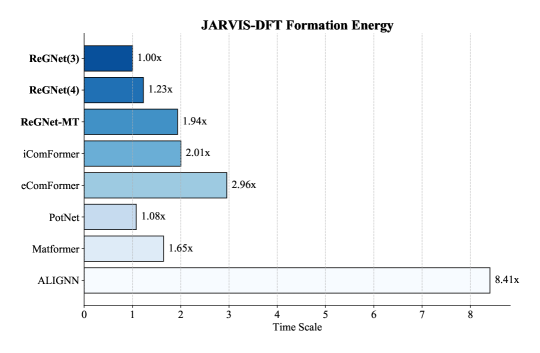
Figure 5: Efficiency comparison of training time per epoch, with each method’s training time scaled relative to ReGNet(3). 3 and 4 indicate the number of ReGNet blocks.

B.5 Full Ablation on JARVIS Dataset

Table 9: Ablation on our method with/without reciprocal space information and model depth in terms of test MAE on JARVIS dataset. 3 and 4 indicate the number of ReGNet blocks. The best results are shown in bold.

	Form. Energy	Bandgap(OPT)	$E_{total}$	Bandgap(MBJ)	$E_{hull}$
Method	meV/atom	eV	meV/atom	eV	meV
ReGNet w/o Reciprocal(3)	29.6	0.135	32.5	0.295	68.8
ReGNet(3)	27.8	0.127	27.2	0.242	52.9
ReGNet(4)	27.0	0.127	26.8	0.239	48.0

In addition to the primary results, we conduct an ablation study to assess the impact of incorporating reciprocal space information in ReGNet using the JARVIS dataset. As shown in Table˜9, integrating reciprocal space information consistently improves performance across all evaluated properties. Notably, ReGNet with reciprocal space information outperforms its counterpart without it, achieving significant gains in predictive accuracy for total energy and Ehull. The model with four ReGNet blocks achieves better result than the one with three blocks, highlighting the importance of both reciprocal space features and model depth in improving prediction accuracy.

B.6 Training Time Scale Efficiency Analysis

Beyond the superior modeling capacity for crystalline materials, our ReGNet is faster and more efficient than previous works. To demonstrate the efficiency of ReGNet, we compare ReGNet and its multi-task variant ReGNet-MT with iComFormer, eComFormer, PotNet, Matformer, and ALIGNN. Evaluation is in terms of training time per epoch on the task of JARVIS formation energy prediction. From Figure˜5, ReGNet demonstrates superior computational efficiency. Specifically, ReGNet(3) outperforms iComFormer by 1.77$\times$, eComFormer by 2.96$\times$, PotNet by 1.08$\times$, Matformer by 1.65$\times$, and ALIGNN by 8.41$\times$ speedup. Finally, the time for ReGNet-MT predicting 5 properties does not even double. These results highlight the effectiveness of ReGNet in reducing computational overhead while maintaining performance in prediction as previously mentioned.

References

- Ashcroft & Mermin (2001) Neil W. Ashcroft and N. David Mermin. Solid State Physics. Harcourt College Publishers, 2001.
- Ashcroft et al. (1978) Neil W Ashcroft, N David Mermin, and Sergio Rodriguez. Solid state physics. American Journal of Physics, 46(1):116–117, 1978.
- Beaini et al. (2023) Dominique Beaini, Shenyang Huang, Joao Alex Cunha, Zhiyi Li, Gabriela Moisescu-Pareja, Oleksandr Dymov, Samuel Maddrell-Mander, Callum McLean, Frederik Wenkel, Luis Müller, et al. Towards foundational models for molecular learning on large-scale multi-task datasets. arXiv preprint arXiv:2310.04292, 2023.
- Bloch (1929) Felix Bloch. Über die quantenmechanik der elektronen in kristallgittern. Zeitschrift für physik, 52(7):555–600, 1929.
- Chen et al. (2019) Chi Chen, Weike Ye, Yunxing Zuo, Chen Zheng, and Shyue Ping Ong. Graph networks as a universal machine learning framework for molecules and crystals. Chemistry of Materials, 31(9):3564–3572, 2019.
- Choudhary & DeCost (2021) Kamal Choudhary and Brian DeCost. Atomistic line graph neural network for improved materials property predictions. npj Computational Materials, 7(1):185, 2021.
- Choudhary et al. (2020) Kamal Choudhary, Kevin F Garrity, Andrew CE Reid, Brian DeCost, Adam J Biacchi, Angela R Hight Walker, Zachary Trautt, Jason Hattrick-Simpers, A Gilad Kusne, Andrea Centrone, et al. The joint automated repository for various integrated simulations (jarvis) for data-driven materials design. npj computational materials, 6(1):173, 2020.
- Choudhary et al. (2022) Kamal Choudhary, Brian DeCost, Chi Chen, Anubhav Jain, Francesca Tavazza, Ryan Cohn, Cheol Woo Park, Alok Choudhary, Ankit Agrawal, Simon JL Billinge, et al. Recent advances and applications of deep learning methods in materials science. npj Computational Materials, 8(1):59, 2022.
- Christofidellis et al. (2023) Dimitrios Christofidellis, Giorgio Giannone, Jannis Born, Ole Winther, Teodoro Laino, and Matteo Manica. Unifying molecular and textual representations via multi-task language modelling. In International Conference on Machine Learning, pp. 6140–6157. PMLR, 2023.
- Cullity & Smoluchowski (1957) Bernard Dennis Cullity and R Smoluchowski. Elements of x-ray diffraction. Physics Today, 10(3):50–50, 1957.
- Economou (2010) Eleftherios N. Economou. The Physics of Solids. Springer, 2010.
- Egerton et al. (2005) Ray F Egerton et al. Physical principles of electron microscopy, volume 56. Springer, 2005.
- Elton et al. (2018) Daniel C Elton, Zois Boukouvalas, Mark S Butrico, Mark D Fuge, and Peter W Chung. Applying machine learning techniques to predict the properties of energetic materials. Scientific reports, 8(1):9059, 2018.
- Evgeniou & Pontil (2004) Theodoros Evgeniou and Massimiliano Pontil. Regularized multi–task learning. In Proceedings of the tenth ACM SIGKDD international conference on Knowledge discovery and data mining, pp. 109–117, 2004.
- Gasteiger et al. (2020) Johannes Gasteiger, Janek Groß, and Stephan Günnemann. Directional message passing for molecular graphs. arXiv preprint arXiv:2003.03123, 2020.
- Goodall & Lee (2020) Rhys EA Goodall and Alpha A Lee. Predicting materials properties without crystal structure: deep representation learning from stoichiometry. Nature communications, 11(1):6280, 2020.
- Gross & Marx (2014) Richard Gross and Achim Marx. Festkörperphysik. De Gruyter, 2014.
- James (1963) RW James. The dynamical theory of x-ray diffraction. In Solid State Physics, volume 15, pp. 53–220. Elsevier, 1963.
- Jha et al. (2018) Dipendra Jha, Logan Ward, Arindam Paul, Wei-keng Liao, Alok Choudhary, Chris Wolverton, and Ankit Agrawal. Elemnet: Deep learning the chemistry of materials from only elemental composition. Scientific reports, 8(1):17593, 2018.
- Jones (2015) Robert O Jones. Density functional theory: Its origins, rise to prominence, and future. Reviews of modern physics, 87(3):897–923, 2015.
- Kingma (2014) Diederik P Kingma. Adam: A method for stochastic optimization. arXiv preprint arXiv:1412.6980, 2014.
- Kosmala et al. (2023) Arthur Kosmala, Johannes Gasteiger, Nicholas Gao, and Stephan Günnemann. Ewald-based long-range message passing for molecular graphs. In International Conference on Machine Learning, pp. 17544–17563. PMLR, 2023.
- Ladd et al. (1977) Marcus Frederick Charles Ladd, Rex Alfred Palmer, and Rex Alfred Palmer. Structure determination by X-ray crystallography, volume 233. Springer, 1977.
- Lin et al. (2023) Yuchao Lin, Keqiang Yan, Youzhi Luo, Yi Liu, Xiaoning Qian, and Shuiwang Ji. Efficient approximations of complete interatomic potentials for crystal property prediction. In International Conference on Machine Learning, pp. 21260–21287. PMLR, 2023.
- Liu et al. (2022) Shengchao Liu, Meng Qu, Zuobai Zhang, Huiyu Cai, and Jian Tang. Structured multi-task learning for molecular property prediction. In International conference on artificial intelligence and statistics, pp. 8906–8920. PMLR, 2022.
- Louis et al. (2020) Steph-Yves Louis, Yong Zhao, Alireza Nasiri, Xiran Wang, Yuqi Song, Fei Liu, and Jianjun Hu. Graph convolutional neural networks with global attention for improved materials property prediction. Physical Chemistry Chemical Physics, 22(32):18141–18148, 2020.
- Poeppelmeier (2023) Kenneth R Poeppelmeier. Comprehensive Inorganic Chemistry III. Elsevier, 2023.
- Ren et al. (2024) Yuxuan Ren, Dihan Zheng, Chang Liu, Peiran Jin, Yu Shi, Lin Huang, Jiyan He, Shengjie Luo, Tao Qin, and Tie-Yan Liu. Physical consistency bridges heterogeneous data in molecular multi-task learning. arXiv preprint arXiv:2410.10118, 2024.
- Riquelme et al. (2021) Carlos Riquelme, Joan Puigcerver, Basil Mustafa, Maxim Neumann, Rodolphe Jenatton, André Susano Pinto, Daniel Keysers, and Neil Houlsby. Scaling vision with sparse mixture of experts. Advances in Neural Information Processing Systems, 34:8583–8595, 2021.
- Rupp et al. (2012) Matthias Rupp, Alexandre Tkatchenko, Klaus-Robert Müller, and O Anatole Von Lilienfeld. Fast and accurate modeling of molecular atomization energies with machine learning. Physical review letters, 108(5):058301, 2012.
- Schütt et al. (2017) Kristof Schütt, Pieter-Jan Kindermans, Huziel Enoc Sauceda Felix, Stefan Chmiela, Alexandre Tkatchenko, and Klaus-Robert Müller. Schnet: A continuous-filter convolutional neural network for modeling quantum interactions. Advances in neural information processing systems, 30, 2017.
- Schütt et al. (2018) Kristof T Schütt, Huziel E Sauceda, P-J Kindermans, Alexandre Tkatchenko, and K-R Müller. Schnet–a deep learning architecture for molecules and materials. The Journal of Chemical Physics, 148(24), 2018.
- Shazeer et al. (2017) Noam Shazeer, Azalia Mirhoseini, Krzysztof Maziarz, Andy Davis, Quoc Le, Geoffrey Hinton, and Jeff Dean. Outrageously large neural networks: The sparsely-gated mixture-of-experts layer. arXiv preprint arXiv:1701.06538, 2017.
- Smith & Topin (2019) Leslie N Smith and Nicholay Topin. Super-convergence: Very fast training of neural networks using large learning rates. In Artificial intelligence and machine learning for multi-domain operations applications, volume 11006, pp. 369–386. SPIE, 2019.
- Staacke et al. (2021) Carsten G Staacke, Hendrik H Heenen, Christoph Scheurer, Gábor Csányi, Karsten Reuter, and Johannes T Margraf. On the role of long-range electrostatics in machine-learned interatomic potentials for complex battery materials. ACS Applied Energy Materials, 4(11):12562–12569, 2021.
- Taniai et al. (2024) Tatsunori Taniai, Ryo Igarashi, Yuta Suzuki, Naoya Chiba, Kotaro Saito, Yoshitaka Ushiku, and Kanta Ono. Crystalformer: infinitely connected attention for periodic structure encoding. arXiv preprint arXiv:2403.11686, 2024.
- Unke et al. (2021) Oliver T Unke, Stefan Chmiela, Michael Gastegger, Kristof T Schütt, Huziel E Sauceda, and Klaus-Robert Müller. Spookynet: Learning force fields with electronic degrees of freedom and nonlocal effects. Nature communications, 12(1):7273, 2021.
- Wang et al. (2021) Anthony Yu-Tung Wang, Steven K Kauwe, Ryan J Murdock, and Taylor D Sparks. Compositionally restricted attention-based network for materials property predictions. Npj Computational Materials, 7(1):77, 2021.
- Xiao et al. (2024) Peiyao Xiao, Hao Ban, and Kaiyi Ji. Direction-oriented multi-objective learning: Simple and provable stochastic algorithms. Advances in Neural Information Processing Systems, 36, 2024.
- Xie & Grossman (2018) Tian Xie and Jeffrey C Grossman. Crystal graph convolutional neural networks for an accurate and interpretable prediction of material properties. Physical review letters, 120(14):145301, 2018.
- Yan et al. (2022) Keqiang Yan, Yi Liu, Yuchao Lin, and Shuiwang Ji. Periodic graph transformers for crystal material property prediction. Advances in Neural Information Processing Systems, 35:15066–15080, 2022.
- Yan et al. (2024) Keqiang Yan, Cong Fu, Xiaofeng Qian, Xiaoning Qian, and Shuiwang Ji. Complete and efficient graph transformers for crystal material property prediction. arXiv preprint arXiv:2403.11857, 2024.
- Yu et al. (2022) Hongyu Yu, Liangliang Hong, Shiyou Chen, Xingao Gong, and Hongjun Xiang. Capturing long-range interaction with reciprocal space neural network. arXiv preprint arXiv:2211.16684, 2022.
- Zeni et al. (2023) Claudio Zeni, Robert Pinsler, Daniel Zügner, Andrew Fowler, Matthew Horton, Xiang Fu, Sasha Shysheya, Jonathan Crabbé, Lixin Sun, Jake Smith, et al. Mattergen: a generative model for inorganic materials design. arXiv preprint arXiv:2312.03687, 2023.
- Ziman (2001) John M Ziman. Electrons and phonons: the theory of transport phenomena in solids. Oxford university press, 2001.