Tomographic halo model of the unWISE-Blue galaxies using cross-correlations with BOSS CMASS galaxies

Abstract

The halo model offers a framework for investigating galaxy clustering, and for understanding the growth of galaxies and the distribution of galaxies of different types. Here, we use the halo model to study the small-scale clustering and halo occupation distribution (HOD) of the unWISE-Blue galaxy sample, an infrared-selected sample of $\sim$100 million galaxies across the entire extragalactic sky at $z\sim 0.5$ – similar redshifts to the Baryon Oscillation Spectroscopic Survey (BOSS) CMASS sample. Although the photometric unWISE galaxies cannot be easily split in redshift, we use their cross-correlation with the BOSS CMASS sample to tomographically probe the HOD of the unWISE galaxies at $0.45<z<0.75$. To do so, we develop a new method for applying the halo model to cross-correlations between a photometric sample and a spectroscopic sample in narrow redshift bins, incorporating halo exclusion, post-Limber corrections, and redshift-space distortions. We reveal strong evolution in the CMASS HOD, and modest evolution in the unWISE-Blue HOD. For unWISE-Blue, we find that the average bias and mean halo mass drop from $b=1.6$ and $\log_{10}(M_{\mathrm{h}}/M_{\odot})\sim 13.4$ at $z\sim 0.5$ to $b=1.4$ and $\log_{10}(M_{\mathrm{h}}/M_{\odot})\sim 13.1$ at $z\sim 0.7$, and that the satellite fraction drops modestly from $\sim$20% to $\sim$10% in the same range. These results are useful for creating mock samples of the unWISE-Blue galaxies. Furthermore, the techniques developed to obtain these results are applicable to other tomographic cross-correlations between photometric samples and narrowly-binned spectroscopic samples, such as clustering redshifts.

1 Introduction

Over a period of 10 years, the Wide-field Infrared Survey Explorer satellite (WISE; Wright et al., 2010) mapped the sky in the infrared, initially in four wavebands for the first year with active cooling, and then in two bands, at 3.4 and 4.6 $\mu$m, for the remaining nine years (the NEOWISE post-cryogenic survey; Mainzer et al., 2011, 2014). This survey has produced several very large catalogs of infrared sources, such as the unWISE catalog of 2 billion sources from the first five years of observations (Schlafly et al., 2019). A simple infrared color cut and the use of Gaia data to reject bright point sources yields a sample of 500 million galaxies at $0<z<2$ across the entire sky. The high number density and full sky coverage make unWISE an ideal sample for cross-correlations with other full-sky tracers, e.g. CMB secondary anisotropies such as lensing (Krolewski et al., 2020, 2021; Kusiak et al., 2022; Farren et al., 2024, 2023), the kinetic Sunyaev-Zel’dovich effect (Kusiak et al., 2021; Bloch & Johnson, 2024), the integrated Sachs-Wolfe effect (Krolewski & Ferraro, 2022), and other full-sky samples like high-energy neutrinos (Ouellette & Holder, 2024) and the cosmic infrared backgpround (Yan et al., 2024). To make further use of this sample, we must clearly understand the types of galaxies it contains.

To this end we employ the halo model, a framework for understanding the distribution of galaxies within the large-scale cosmic web (Seljak, 2000; Ma & Fry, 2000; Peacock & Smith, 2000; Cooray & Sheth, 2002; Smith et al., 2002). In the halo model, galaxies exist only within halos of dark matter, where each halo may have at most one central galaxy and an arbitrary number of satellite galaxies. The distribution of central and satellite galaxies within a halo, and the distribution of halos that host each type of galaxy, are controlled by the halo occupation distribution (HOD; Berlind et al., 2003; Zehavi et al., 2005; Zheng et al., 2007). Different HOD types are required for different galaxy types. Here, we adopt a strict halo model where halos are assumed to be spherical, and we use analytic expressions or numerical fits for the halo density profile, halo mass function, matter power spectrum, halo bias, concentration-mass relation and an exclusion model to account for overlaps between halos. The details are given in Section 4.1.

By fitting the parameters of the halo model to the clustering of the unWISE sample, we can determine the basic properties of these galaxies within the halo model framework. The unWISE galaxies are split into three samples at $z\sim 0.5$, $1.1$, and $1.5$ using a simple color cut (Schlafly et al., 2019; Krolewski et al., 2020). As a first step towards modelling their HOD, we consider the lowest-redshift “Blue” sample, with a broad redshift distribution centered at $z\sim 0.5$ and extending to $z\sim 1$. The sample includes galaxies across a wide range in redshift, but further subdivision in $z$ is not possible because the two-band WISE photometry cannot be used to construct accurate photometric redshifts. Cross-matching to optical imaging surveys would improve this situation, but would considerably reduce the sky coverage and decrease the number density, both of which are undesirable for many cross-correlation applications.

In order to understand the tomographic clustering, we consider the cross-correlation with the spectroscopic Sloan Digital Sky Survey (SDSS; York et al., 2000) Baryon Oscillation Spectroscopic Survey (BOSS; Dawson et al., 2013) CMASS galaxies (see Section 2.2 for details of this sample). By dividing CMASS into many narrow redshift bins and cross-correlating with unWISE, we can measure unWISE clustering tomographically, without requiring photometric redshifts for the unWISE galaxies. This approach is conceptually similar to clustering redshifts (Newman, 2008; McQuinn & White, 2013; Ménard et al., 2013).

This allows us to go beyond the limits of a photometric sample, enhancing our ability to understand the evolution of the sample with redshift. The correlation and cross-correlation measurements are presented in Section 3. The extensions to the halo model required to probe the cross-correlation are presented in Section 4.3. The resulting HOD constraints are presented in Section 5. As a by-product of our analysis we fit the CMASS galaxies, matching previous results (White et al., 2011; Alam et al., 2017; Reid et al., 2014; Saito et al., 2016). For the unWISE galaxies, we find evidence for a strongly evolving HOD, and we are able to compare the host halos of unWISE and CMASS galaxies. These results are discussed further in our conclusions, summarized in Section 6.

2 Data

2.1 unWISE

The WISE satellite mapped the entire sky at 3.4 (W1), 4.6 (W2), 12 (W3), and 22 (W4) $\mu$m for one year in the main mission (Wright et al., 2010), and subsequently for nine additional years in W1 and W2 for the non-cryogenic post-hibernation NEOWISE phase (Mainzer et al., 2011, 2014). This deep all-sky infrared imaging is ideal for identifying large samples of $z\gtrsim 1$ galaxies: the unWISE catalog (Lang, 2014; Meisner et al., 2017) contains 500 million galaxies across the entire sky. With a simple W1-W2 color cut, these galaxies can be divided into three samples at different redshifts, the Blue, Green, and Red samples at $z\sim 0.5$, 1.1, and 1.5, respectively. These samples are extensively described in Krolewski et al. (2020) and Schlafly et al. (2019), and their properties are summarized in Table 1 of Krolewski et al. (2020). Stars are removed by matching to Gaia DR2 (Gaia Collaboration et al., 2018) and removing any unWISE source within $2.75^{\prime\prime}$ of a Gaia point source. Residual stellar contamination is $<2\%$. We directly measure the slope of the number counts, $s\equiv d\log_{10}(N/\mathrm{d}m)$, by perturbing the photometry of the unWISE galaxies and applying the same color cuts (see Appendix D of Krolewski et al., 2020).

We measure the unWISE redshift distribution using the COSMOS2015 photometric redshifts in the 2 deg² COSMOS field (Fig. 1; Laigle et al., 2016). We use the photometric redshift from the nearest COSMOS source within $2.75^{\prime\prime}$ (1 WISE pixel), first removing any COSMOS source fainter than 20.7 (19.2) Vega magnitude at 3.6 (4.2) $\mu$m; this is necessary to eliminate spurious matches caused by blends in WISE, which has a $6^{\prime\prime}$ PSF. We use the median of the redshift likelihood distribution for each source, replacing it with the redshift from the AGN fit if the SED is better fit by an AGN. AGN contamination is low, especially for the Blue sample that we fit in this work, both because AGN mid-infrared colors are different from the Blue color cuts, and because the Gaia point-source cut removes the brightest quasars. Ultimately, only 19% of the COSMOS matches are better-fit by an AGN SED.

We additionally apply the linear imaging systematics weights described in Krolewski & Ferraro (2022) and Farren et al. (2024) to correct for spurious correlations between unWISE galaxy density and WISE depth and stellar density. After applying these weights, the unWISE galaxy density is uncorrelated with nine imaging systematics templates (WISE depth, extinction, dust density, and DIRBE estimates of diffuse infrared sky background).

2.2 CMASS

The Baryon Oscillation Spectroscopic Survey (BOSS; Dawson et al., 2013; Eisenstein et al., 2011) targeted 1.5 million galaxies, stars and quasars selected from 10,000 deg² of SDSS DR8 imaging (Gunn et al., 1998; York et al., 2000; Gunn et al., 2006; Fukugita et al., 1996; Lupton et al., 2001; Smith et al., 2002; Pier et al., 2003; Padmanabhan et al., 2008; Doi et al., 2010; Aihara et al., 2011). The upgraded BOSS spectrograph (Smee et al., 2013) enabled highly accurate and complete redshifts for these targets. The majority of the targets are luminous red galaxies at $0.2<z<0.75$, composing the CMASS and LOWZ samples. Successful redshifts are assembled into a uniformly-selected large-scale structure catalog in Reid et al. (2016).

In this paper, we use the CMASS galaxies as a spectroscopic tracer to tomographically probe the halo occupation distribution of the unWISE galaxies across a broad range of redshifts. We therefore measure the cross-correlation between unWISE galaxies and six bins from CMASS with $\Delta z=0.05$ from $z=0.45$ to 0.75. We restrict the clustering measurement to the union of the CMASS LSS mask and the unWISE mask. $\sim$75% of the CMASS sample is located in the North Galactic Cap (NGC). As the sample is slightly different in the South Galactic Cap (SGC), we restrict our measurement to the NGC for simplicity; the additional constraining power from SGC is minimal, and may require different HOD parameters due to the slightly different selection.

Like unWISE, the CMASS galaxy density must be corrected for its dependence on imaging systematics. It is also affected by fiber collisions: no galaxy pairs with separation $<55$” can be observed due to the physical size of the BOSS spectrograph fibers. Galaxies lost to fiber collisions tend to occupy overdense environments; therefore, accurately measuring the clustering requires correcting for fiber collisions. Like the imaging systematics, fiber collisions are approximately mitigated in the catalog by creating another set of weights, upweighting the nearest neighbor to a collided galaxy. We apply the default weights in the catalog,

$$w_{\textrm{tot}}=w_{\textrm{systot}}(w_{\textrm{cp}}+w_{\textrm{noz}}-1).$$ (1)

We also restrict our autocorrelation measurements to scales larger than the 55” collision scale (corresponding to 0.3 $h^{-1}$ Mpc at $z=0.45$ and 0.5 $h^{-1}$ Mpc at $z=0.75$).

Finally, due to the broad redshift kernel of the unWISE galaxies, we must account for magnification of CMASS galaxies by foreground unWISE galaxies, which depends on the number counts slope $s$ for CMASS. We determine $s$ by uniformly shifting the CMASS galaxies’ flux across all bands, and by accounting for the change in redshift success rate from lensing magnification. We then apply the CMASS targeting color cuts to the shifted photometry. Measurements of $s$ for CMASS are given in Appendix D of Farren et al. (2024), and are very similar to the measurements in Wenzl et al. (2023). We reproduce the magnification bias measurements in Table 1, and use $s=0.453$ for the unWISE-Blue sample.

$z_{\textrm{min}}$	$z_{\textrm{max}}$	$s$
0.45	0.50	0.937
0.50	0.55	1.040
0.55	0.60	1.148
0.60	0.65	1.352
0.65	0.70	1.553
0.70	0.75	1.957

Table 1: Magnification bias coefficient $s$ for the different CMASS redshift bins, reproducing Table 13 in Farren et al. (2024). We use $s=0.453$ for the unWISE-Blue sample.

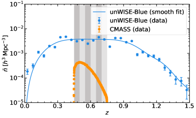
Figure 1: Number densities of unWISE-Blue (blue) and CMASS (orange) galaxy samples. The gray shaded regions demarcate the different redshift bins. Uncertainties on the unWISE-Blue $\bar{n}(z)$ are from Poisson fluctuations in the observed photo-$z$ number counts in the 2 deg² COSMOS field.

3 CMASS-unWISE cross-correlation measurement

We use the Davis-Peebles estimator (Davis & Peebles, 1983),

$$w_{12}(\theta)=\frac{D_{s}D_{p}}{D_{s}R_{p}}\frac{N_{R}}{N_{D}}-1,$$ (2)

to compute the cross-correlation in 10 log-spaced bins between 0.1 and 10 $h^{-1}$ Mpc at the mean redshift of each bin. We use a tree-based correlation function code to store the shared unWISE data and random catalogs across all redshift bins. The unWISE randoms are distributed within the unWISE mask, with the expected number of randoms in each pixel scaled using the sub-pixel mask accounting for area lost within each NSIDE=2048 HEALPix (Górski et al., 2005) pixel due to diffraction spikes, latents, or ghosts around modestly bright WISE sources.

We use jackknife resampling to compute the covariance matrix (see Mohammad & Percival (2022) for discussion on the accuracy of the jackknife covariance). We create jackknife regions by splitting the sky into NSIDE=8 HEALPix pixels, and then joining neighboring pixels until the regions are roughly the same size. This produces 136 jackknife regions. The error on $w_{12}(\theta)$ becomes

$$\sigma^{2}_{w}(\theta)=\sum_{L=1}^{N}\frac{R_{[L]}}{R}\left(w_{[L]}(\theta)-w(\theta)\right)^{2},$$ (3)

where $R$ refers to the numbers of randoms, the subscript $[L]$ indicates that we exclude the $L$th region (correcting the conventional jackknife factor for the fact that the regions are slightly different sizes; see Equation 5 in Myers et al. (2005)), and $w(\theta)$ is simply the measured cross-correlation using the full sky. We use the same jackknife regions for both the auto and cross-correlations, allowing us to compute the full covariance matrix between all spatial bins and between the auto and cross-correlations (Fig. 2).

Due to the finite number of jackknife realizations, there is a sample variance associated with the covariance matrix. This noise biases the expectation value of the inverse covariance matrix (Hartlap et al., 2007; Dodelson & Schneider, 2013; Percival et al., 2014; Sellentin & Heavens, 2016) and changes the form of the likelihood (Percival et al., 2022). We use the Gaussian approximation of Percival et al. (2022), following their Equations 54–56 to modify the covariance matrix.

The correlation function is normalized using the galaxy density across the entire survey area. However, the survey area is finite, meaning galaxy density across the survey area is not necessarily equal to the true galaxy density across the entire Universe. This can be corrected by subtracting the integral constraint, calculated by (Roche & Eales, 1999; Coil, 2013)

$$\mathrm{IC}=\frac{1}{\Omega^{2}}\iint w(\theta)\;\mathrm{d}\Omega_{1}\>\mathrm{d}\Omega_{2},$$ (4)

where $\Omega$ is the area of the survey and the integrals run over the survey window function. To study the size of the integral constraint, we compute it for a single example redshift bin, $0.45<z<0.50$, using CAMB (Lewis et al., 2000; Howlett et al., 2012) to compute $w(\theta)$ (out to very large scales) from the nonlinear power spectrum times fiducial linear biases of 1.87 and 1.68 appropriate for unWISE-Blue and CMASS. We find the integral constraint is 1.6% of the cross-correlation in the largest bin ($8<r<10$ $h^{-1}$ Mpc) and negligible compared to the much larger CMASS autocorrelation. This is equal to 0.3$\sigma$ for the final bin cross-correlation, i.e. considerably smaller than the statistical error. Due to the small size of the integral constraint, we neglect it hereafter.

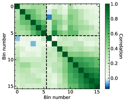
Figure 2: The jackknife correlation matrix for the $0.5<z<0.55$ redshift bin, with axes labelled by bin number. The black dotted lines separate the matrix into its component blocks: the upper left block is the CMASS autocorrelation matrix while the lower right block is the CMASS-unWISE cross-correlation matrix. The autocorrelation matrix has fewer elements due to the small-scale cut removing scales affected by fiber collisions.

4 The HOD model

In this section, we describe the HOD model used to jointly characterize the CMASS autocorrelation and CMASS-unWISE cross-correlation data. We begin by taking a step back and examining halo model described in Murray et al. (2021) (see also the recent review in Asgari et al. (2023)), whose HALOMOD code we use and modify.

4.1 Halo model

The halo model states that at large scales, all matter is bound to “halos” of dark matter. It is assumed that each halo is spherically symmetric and that halo shape depends solely on halo mass. This implies that the halo density is a strictly a function of halo mass and distance from the halo center, i.e. $\rho_{\mathrm{h}}=\rho_{\mathrm{h}}(r,M)$. Therefore, the density field in a region of the Universe that contains $n$ halos is

$$\rho(\bm{x})=\sum_{i=1}^{n}\rho_{\mathrm{h}}(|\bm{x}-\bm{x}_{i}|,M_{i}),$$ (5)

where $\bm{x}_{i}$ and $M_{i}$ are the position of the center and mass, respectively, of the $i$th halo. However, this function is difficult to compute in practice. The power of the halo model lies in its ability to convert Equation (5) into a semi-analytic form that can be readily calculated computationally. To do so, the halo model requires the following pieces of information:

• The moments of the halo density profiles ($\langle\rho_{\mathrm{h}}(r,M)\rangle$, $\langle\rho_{\mathrm{h}}^{2}(r,M)\rangle$, etc.). We use the Navarro-Frenk-White profile (Navarro et al., 1997).

• The halo mass function (HMF) $n(M)$, which provides the abundance of halos of a given mass. We use the Tinker et al. (2008) mass function. Masses are reported in their default units, spherical overdensity masses with $\Delta=200$ relative to the matter density.

• The matter overdensity

  $$\delta(\bm{x})\equiv\frac{\rho(\bm{x})-\bar{\rho}}{\bar{\rho}},$$ (6)

  where $\bar{\rho}$ is the mean of $\rho(\bm{x})$. This is set by the cosmology and primordial power spectrum; we use a Planck 2015 (Planck Collaboration et al., 2016) cosmology with $\sigma_{8}=0.831$, $n_{s}=0.9645$, and the nonlinear power spectrum from Takahashi et al. (2012).

• The halo bias $b_{\mathrm{h}}(\bm{x},M)$, which is the expected overdensity of halos of mass $M$ in a region with matter overdensity $\delta(\bm{x})$. We use the mass-bias relation of Tinker et al. (2010), and additionally allow for a scale-dependent bias following Tinker et al. (2005).

• The concentration-mass relation $c(M)$, which describes the link between halo shape and halo mass. We use the formulation of Duffy et al. (2008).

• A “halo exclusion” model to account for double counting of correlations within halos in both the 1-halo and 2-halo terms of the halo model. This is necessary to accurately model the transition region between the 1-halo and 2-halo terms, both of which are relevant to the scales of this work. Halo exclusion has previously been difficult to model. Using the NgMatched model of Tinker et al. (2005), we model exclusion between triaxial ellipsoids with a range of axis ratios. This method is cumbersome because it requires double integrals over both halo mass distributions at every wavenumber; it is simplified by calculating the number density with 2D integrals and then matching the number density in separable 1D integrals elsewhere.

4.2 HOD for cross-correlations

Thus far, the framework of the halo model considers only the bulk properties of halos, meaning each halo is essentially featureless beyond its density profile. To add galaxies to the halo model, we must specify $N(M)$, the HOD function that describes the number of galaxies that populate a halo of mass $M$.

In this paper, we use the HOD model developed in Zheng et al. (2007), which states that

$$\langle N(M)\rangle=\langle N_{\mathrm{c}}(M)\rangle+\langle N_{\mathrm{s}}(M)\rangle,$$ (7)

where

$$\langle N_{\mathrm{c}}(M)\rangle=\frac{1}{2}\left[1+\mathrm{erf}\left(\frac{\log M-\log M_{\mathrm{min}}}{\sigma_{\log M}}\right)\right]$$ (8)

and

$$\langle N_{\mathrm{s}}(M)\rangle=\langle N_{\mathrm{c}}(M)\rangle\left(\frac{M-M_{0}}{M_{1}}\right)^{\alpha},$$ (9)

where $\log$ is the base-10 logarithm ($\log_{10}$). $\langle N_{\mathrm{c}}(M)\rangle$ and $\langle N_{\mathrm{s}}(M)\rangle$ are the mean number of central and satellite galaxies, respectively, that one expects to find in a halo of mass $M$. $\langle N_{\mathrm{c}}(M)\rangle$ follows a binomial distribution and ranges between 0 and 1 (since there can be at most one central galaxy), while $\langle N_{\mathrm{s}}(M)\rangle$ follows a Poisson distribution and can be arbitrarily large.

The HOD parameters $M_{\mathrm{min}}$, $M_{0}$, $M_{1}$, $\alpha$, and $\sigma_{\log M}$ control the relationship between halo mass and galaxy number. Specifically (Zheng et al., 2007),

• $M_{\mathrm{min}}$ is the characteristic minimum mass a halo must have to host a central galaxy;

• $M_{0}$ sets a cutoff below which one finds zero satellites;

• $M_{1}$ sets the mass at which one finds one satellite per halo;

• $\alpha$ is the slope of the satellite galaxy number;

• $\sigma_{\log M}$ is the width of the central galaxy cutoff profile.

Moreover, we assume the “central condition” for the CMASS HOD, which requires that halos cannot host a satellite galaxy without also hosting a central. This is physically reasonable because central galaxies are typically more luminous than satellite galaxies, so if the satellite is bright enough to be included in the survey, then the central must be too. We do not assume the central condition for the unWISE-Blue HOD, since unWISE has a bright cut ($\mathrm{W1}>15.5$) that removes a fairly large number of galaxies; hence, the satellite could be in the sample, but the central would be too bright. Practically, this makes very little difference, since the data favors HODs where $N_{\mathrm{s}}$ drops off at much higher masses than $N_{\mathrm{c}}$. The central condition is not compatible with a binomial $N_{\mathrm{c}}$ and a Poissonian $N_{\mathrm{s}}$ (Beutler et al., 2013); the Poisson distribution for $N_{\mathrm{s}}$ is therefore modified to satisfy the central condition as shown in Table 3 of Asgari et al. (2023).

When considering cross-correlations, we must also consider the correlations between centrals and satellites of the two galaxy populations: if one sample inhabits a halo, is the other sample more or less likely to also inhabit that halo? These correlations are parameterized by $R_{\mathrm{cs}}$, $R_{\mathrm{ss}}$, and $R_{\mathrm{sc}}$, which are correlation coefficients controlling correlations between centrals and satellites of each type (Miyaji et al., 2011; Krause et al., 2013). For simplicity, we fix all three parameters to zero (the uncorrelated case); exploring the impact of these parameters is left for future work.

The Zheng et al. (2007) model assumes that at high mass, every halo hosts a central galaxy ($N_{\mathrm{c}}(M)=1$). However, CMASS has color cuts and flux limits creating incompleteness: the color cuts can reduce completeness at high mass while the flux limits generally reduce completeness at low mass and high redshift. The impact of flux limits is studied in Zhai et al. (2017) and Tinker et al. (2017), who find that the Zheng et al. (2007) HOD can reproduce the real galaxy occupation very well at low mass, largely by changing $M_{\textrm{min}}$ and $\sigma_{\log M}$. The impact of color cuts is studied in Leauthaud et al. (2016), who directly quantify CMASS completeness by comparing the CMASS stellar mass function to the stellar mass function of a massive galaxy sample selected without color cuts. At $z<0.6$, color cuts remove galaxies from CMASS even at the massive end, causing $N_{\mathrm{c}}(M)$ to asymptote to 30–50% below unity. This can be modelled by uniformly reducing $N(M)$ by a scaling factor $f_{\textrm{inc}}$, the asymptotic completeness at the high stellar-mass end. Leauthaud et al. (2016) report $f_{\textrm{inc}}$ in several redshift bins across the CMASS range; we reproduce their calculation using our exact redshift bins, using their publicly available data (Bundy et al., 2015). Specifically, we linearly interpolate their double-Schechter function fits for the total stellar mass function (Table 1 of Leauthaud et al. (2016)); measure the CMASS stellar mass function in a given redshift bin using their Stripe 82 catalog and masses, requiring a match to CMASS; and determine $f_{\textrm{inc}}$ by fitting the completeness $c$ as a function of $M_{\star}$ by (their Equation 17):

$$c=\frac{f_{\textrm{inc}}}{2}\left[1+\mathrm{erf}\left(\frac{\log(M_{*}/M_{1})}{\sigma}\right)\right].$$ (10)

with free parameters $f_{\textrm{inc}}$, $M_{1}$, and $\sigma$. We then apply this $f_{\textrm{inc}}$ scaling factor to $N_{\mathrm{c}}(M)$ in our implementation of the halo model.

Likewise, it is also possible that the unWISE sample does not include every central galaxy, i.e. $N_{\mathrm{c}}<1$ at high mass. unWISE also includes a bright cut, which could remove high-mass halos. Unlike CMASS, detailed studies such as Leauthaud et al. (2016) have not been performed, so the high-mass incompleteness is unknown. To encompass a range of possibilities, we will consider two limiting cases: in one (the default case), we require that the model matches the observed unWISE $\bar{n}(z)$ within the uncertainty (hence $N_{\textrm{c}}=1$ at high mass), and in the other, we impose the observed $\bar{n}(z)$ as a lower bound on the model $\bar{n}(z)$ (hence $N_{\textrm{c}}<1$ at high mass), equivalent to marginalizing over $f_{\textrm{inc}}$ with an uninformative prior. More complicated possibilities are certainly possible, for instance a Gaussian distribution for $N_{\textrm{c}}$ (e.g. Rocher et al., 2023), but they are beyond the scope of this paper, in which we only consider the Zheng et al. (2007) model as a first step in modelling the unWISE-Blue HOD. Within this model, the two cases considered span the uncertainty in unWISE incompleteness.

4.3 Angular cross-correlations

With the specifics of the HOD established, we turn our attention to angular correlations. Considering two galaxy fields, hereafter labelled 1 and 2., the two-point angular correlation function for these fields is given by (e.g. Murray et al., 2021)

$$w_{12}(\theta)\approx\int_{0}^{\infty}\int_{0}^{\infty}p(r_{1})p(r_{2})\xi_{12}(R,\bar{r})\>\mathrm{d}r_{1}\>\mathrm{d}r_{2},$$ (11)

where

$$p_{i}(r)\equiv\frac{\mathrm{d}N_{i}}{\mathrm{d}r}$$ (12)

is the probability density of finding a galaxy from the field $i$ at a line-of-sight comoving distance of $r$, $\xi_{12}$ is the two-point spatial correlation function for the fields 1 and 2,

$$R\equiv\sqrt{r_{1}^{2}+r_{2}^{2}-2r_{1}r_{2}\cos\theta}$$ (13)

is the projected separation between the points $r_{1}$ and $r_{2}$, and

$$\bar{r}\equiv\frac{r_{1}+r_{2}}{2}$$ (14)

is the the mean line-of-sight comoving distance.

4.3.1 Beyond the Limber approximation

To facilitate numerical calculations of $w_{12}$, Equation 11 is often approximated to a more computationally tractable form. For many surveys, each $p_{i}(r)$ is a broad distribution in redshift, and $\theta$ is a small angle, meaning it is appropriate to employ the approximation developed in Limber (1953). However, Limber’s equation diverges for narrow galaxy bins and wide angles (Simon, 2007). While we work on small scales in this paper, our spectroscopic bins are very narrow, with $\Delta z=0.05$. Hence, the Limber approximation is insufficient, and we apply the post-Limber formulation developed by Simon (2007):

$$w_{12}(\theta)\approx\frac{1}{1+\cos\theta}\;{\times}\\ \int_{0}^{\infty}\int_{\sqrt{2(1-\cos\theta)}\bar{r}}^{2\bar{r}}Q(\bar{r},\Delta)\xi_{12}(R,\bar{r},\mu)\frac{R}{\Delta}\>\mathrm{d}R\>\mathrm{d}\bar{r},$$ (15)

where

$$\Delta\equiv\frac{1}{\sqrt{2}}\sqrt{\frac{R^{2}-2\bar{r}^{2}(1-\cos\theta)}{1+\cos\theta}}$$ (16)

and

$$Q(\bar{r},\Delta)\equiv p_{1}(\bar{r}-\Delta)p_{2}(\bar{r}+\Delta)+p_{1}(\bar{r}+\Delta)p_{2}(\bar{r}-\Delta),$$ (17)

while $\mu$ is the cosine of the angle between $R$ and $\bar{r}$.

4.3.2 Redshift-space distortions

We also include the effect of redshift-space distortions (RSD) in the model by allowing $\xi_{12}$ to be a function of separation $R$, angle $\mu$, and comoving distance $\bar{r}$ (or equivalently redshift). Since the effects of RSD are small, we implement a linear model (Kaiser, 1987) where $\xi_{12}$ in Equation 15 takes the form

$$\xi_{12}(R,\bar{r},\mu)=\sum_{\ell\in\{0,2,4\}}\alpha_{\ell}(\beta_{1},\beta_{2})\xi_{12}^{\ell}(R,\bar{r})L_{\ell}(\mu),$$ (18)

where the RSD parameter $\beta\equiv f/b$ and $f$ is the growth factor, commonly approximated as $\Omega_{m}(z)^{0.55}$. Allowing for the cross-correlation of two tracers with differing biases, the coefficients $\alpha$ are:

$$\alpha_{0} =1+\frac{1}{3}(\beta_{1}+\beta_{2})+\frac{1}{5}\beta_{1}\beta_{2},$$ (19)

$$\alpha_{2} =\frac{2}{3}(\beta_{1}+\beta_{2})+\frac{4}{7}\beta_{1}\beta_{2},$$ (20)

$$\alpha_{4} =\frac{8}{35}\beta_{1}\beta_{2},$$ (21)

and the multipole moments of the correlation function are

$$\xi_{\ell}(R,\bar{r})=\frac{i^{\ell}}{2\pi^{2}}\int_{0}^{\infty}P_{12}(k,\bar{r})j_{\ell}(kR)k^{2}\>\mathrm{d}k.$$ (22)

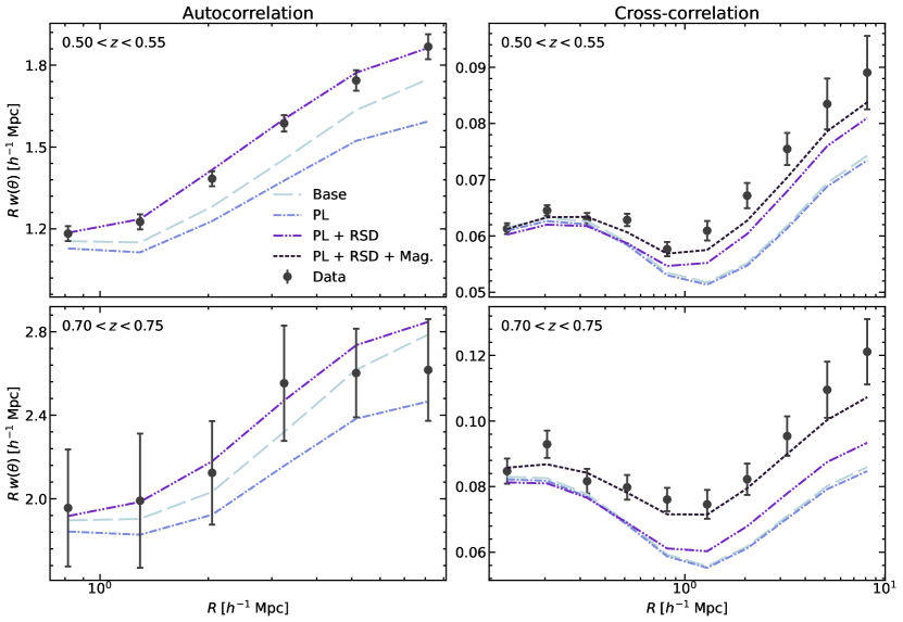
Figure 3: The angular correlation function data and best-fit models for the CMASS autocorrelation (left column) and the CMASS-unWISE cross-correlation (right column) in the redshift bins $0.5<z<0.55$ (top row) and $0.7<z<0.75$ (bottom row), with jackknife errors as described in Section 3. The Base best-fit considers only the standard Limber approximation to $w(\theta)$. In contrast, the PL best-fit uses the post-Limber equation described in Section 4.3.1. Next, the PL + RSD best-fit adds the effects of redshift-space distortion explained in Section 4.3.2. Finally, the PL + RSD + Mag. best-fit includes the magnification bias from Section 4.3.4. Since magnification is negligible for the autocorrelation, we take PL + RSD as the overall best-fit model for the CMASS autocorrelation, and PL + RSD + Mag. as the overall best-fit model for the CMASS-unWISE cross-correlation.

4.3.3 3D power spectrum: one-halo and two-halo terms

Next, we define the model for the 3D power spectrum $P_{12}(k,\bar{r})$ in Equation 22. Within the framework of the halo model, it is convenient to break the power spectrum into a term accounting for intrahalo galaxy correlations (the 1-halo term) and a term accounting for interhalo galaxy correlations (the 2-halo term). In particular, this decomposition is best done in real space, defining $P_{12}(k)$ as the Fourier transform of $\xi_{12}(r)$ (and dropping the redshift label $\bar{r}$ for clarity):

$$P_{12}(k) =4\pi\int_{0}^{\infty}\xi_{12}(r)r^{2}j_{0}(kr)\>\mathrm{d}r,$$ (23)

$$\xi_{12}(r) =[1+\xi_{12}^{1\mathrm{h}}(r)]+\xi_{12}^{2\mathrm{h}}(r),$$ (24)

where $j_{0}(x)=\sin(x)/x$ is the zeroth-order spherical Bessel function. The 1-halo term is given by

$$\xi_{12}^{\mathrm{1h}}(r)=\frac{1}{2\pi^{2}}\int_{0}^{\infty}P_{12}^{\mathrm{1h}}(k)k^{2}j_{0}(kr)\>\mathrm{d}k,$$ (25)

where

$$P_{12}^{\mathrm{1h}}(k)=\int n(M)u(k|M)\Big{[}N_{\mathrm{s},1}N_{\mathrm{s},2}u(k|M)\\ +\langle N_{\mathrm{c},1}N_{\mathrm{s},2}\rangle+\langle N_{\mathrm{c},2}N_{\mathrm{s},1}\rangle\Big{]\>\mathrm{d}M}$$ (26)

is the 1-halo power spectrum, with $u(k|M)$ being the mass-normalised Fourier transform of the halo profile. This form creates a spurious shot-noise power on large scales, which allows the 1-halo term to dominate the 2-halo term on very large scales. We use HALOMOD’s force_1halo_turnover option to remove this term.

The 2-halo term is given by

$$\xi_{12}^{\mathrm{2h}}(r)=\frac{1}{2\pi^{2}}\int_{0}^{\infty}P_{12}^{\mathrm{2h}}(k)k^{2}j_{0}(kr)\>\mathrm{d}k,$$ (27)

where the 2-halo power spectrum is

$$P_{\mathrm{12}}^{2\mathrm{h}}(k)=\iint I_{\mathrm{g}}(k,M_{1})I_{\mathrm{g}}(k,M_{2})\times\\ b(k,M_{2})b(M_{1},r)b(M_{2},r)P_{\mathrm{m}}(k)\>\mathrm{d}M_{1}\>\mathrm{d}M_{2}$$ (28)

and

$$I_{g}(k,M)=\frac{1}{\bar{n}_{g}}n(M)u(k|M)\langle N(M)\rangle.$$ (29)

Note that the $M_{1}$ and $M_{2}$ integrals are separable following the simplifications of the “Ng-Matched” exclusion model (as the triaxial exclusion model otherwise couples the mass limits) as described above in Section 4.1.

4.3.4 Magnification bias

Because unWISE has a very broad galaxy kernel, the cross-correlation arises both from clustered objects at the same redshift, and lensing magnification correlating galaxies at different redshifts. We separately compute the magnification contribution to the angular cross-correlation and add it to the clustering term, using the magnification bias values in Table 1. Since the magnification term is subdominant, for simplicity we do not model it with the halo model, but rather with a simple linear bias times the nonlinear HALOFit (Mead et al., 2021) power spectrum, requiring that the linear bias matches the linear bias of the halo model considered at each point in the MCMC chain.

4.3.5 Binning the angular cross-correlation

We measure the angular cross-correlation as a function of physical scale by converting the angle to a transverse distance using the comoving distance to the mean spectroscopic redshift of each bin, convering $w_{12}(\theta)$ to $w_{12}(R)$. We then compute the binned cross-correlation to compare to the data, averaging $w_{12}(R)$ within each bin in $R$ according to

$$w_{12,\textrm{bin},i}=\frac{1}{R_{\textrm{max},i}^{2}-R_{\textrm{min},i}^{2}}\int_{R_{\textrm{min},i}}^{R_{\textrm{max},i}}2R\,w_{12}(R)\>\mathrm{d}R.$$ (30)

The results of this model model are shown for two example bins at the low and high redshift end in Fig. 3, broken into its constituent terms to demonstrate the effects of the post-Limber, RSD, and magnificantion terms.

4.4 Likelihood

We then compute the standard Gaussian likelihood

$$\mathcal{L}_{\textrm{clus}}=-\frac{1}{2}(\bm{w}_{\textrm{data}}-\bm{w}_{\textrm{mod}})\mathbf{C}^{-1}(\bm{w}_{\textrm{data}}-\bm{w}_{\textrm{mod}})^{T}$$ (31)

where the data vectors run over both CMASS autocorrelation and CMASS-unWISE cross-correlation. We also add two terms of the form

$$\mathcal{L}_{\bar{n}}=-\frac{1}{2}\left(\frac{\bar{n}_{\textrm{mod}}-\bar{n}_{\textrm{data}}}{\sigma_{\bar{n}}}\right)^{2}$$ (32)

to the likelihood for the number density of the CMASS and unWISE galaxies. When marginalizing over the unWISE $f_{\textrm{inc}}$, we do not change the clustering (as this parameter only affects the total number of galaxies), but replace the Gaussian likelihood in $\bar{n}$ with a step function imposing the constraint that $\bar{n}_{\textrm{mod}}>$ $\bar{n}_{\textrm{data}}$.

We sample from the likelihood using the Cobaya MCMC sampler (Torrado & Lewis, 2021), sampling until the errorbars estimated from many sequential chains change by less than 10% when adding a new chain. We impose flat priors on the 10 HOD parameters (five for the CMASS HOD and five for the unWISE-Blue HOD), chosen to be large enough to never be informative.

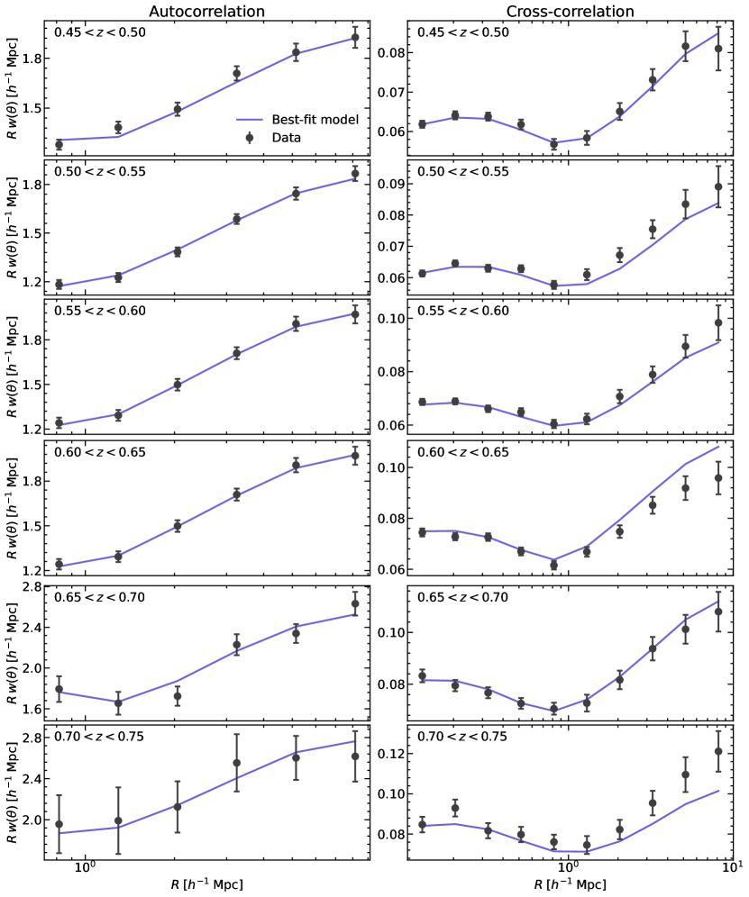
Figure 4: The angular correlation function data and overall best-fit models for the CMASS autocorrelation (left column) and the CMASS-unWISE cross-correlation (right column). From top to bottom, the rows correspond to the redshift bins $0.45<z<0.5$, $0.5<z<0.55$, $0.55<z<0.6$, $0.6<z<0.65$, $0.65<z<0.7$, and $0.7<z<0.75$. The model fits the data well in both autocorrelation and cross-correlation across all redshift bins.

5 HOD constraints

We show the best-fit and median marginalized results, and their errorbars (16th to 84th percentile range) for all HOD parameters and derived parameters in Tables 2 and 3, for the baseline case where unWISE-Blue is assumed to be fully complete ($f_{\textrm{inc}}=1$). We plot the best-fit models in Fig. 4. The model fits the data well in all redshift bins (with 9 degrees of freedom).

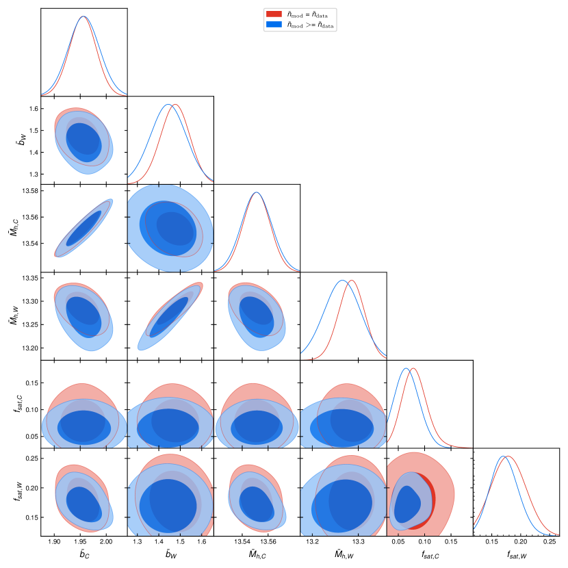
Figure 11: Constraints and degeneracies between the derived parameters at $0.55<z<0.6$. A subscript $C$ denotes the CMASS HOD parameters while a subscript $W$ denotes the unWISE-Blue HOD parameters. The default model is in red, and the model allowing for unWISE incompleteness is in blue.

We plot the evolution of the parameters in Figs. 5 and 6. We show the constraints on the HOD parameters in Fig. 10 and derived parameters in Fig. 11 for a single representative redshift bin at $0.55<z<0.60$. The strong degeneracy directions are very similar between all redshift bins, though the size of the contours increases as the correlation functions become noisier at higher redshift. We therefore only show contours from a single bin for clarity. In this redshift bin, the constraints when requiring the model to match the observed unWISE $\bar{n}$ are considerably stronger than when the observed $\bar{n}$ is only treated as a lower bound. On the other hand, in the first two and last redshift bins, the constraints are very similar to each other regardless of what we assume for the unWISE incompleteness.

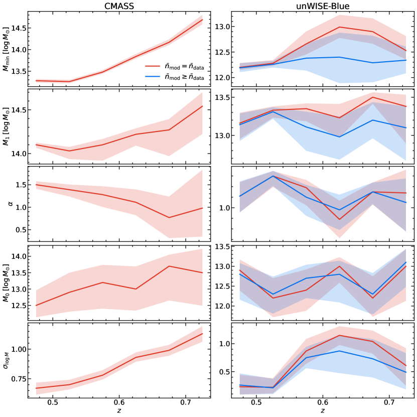
Figure 5: Evolution of the 5 HOD parameters for the CMASS (left column) and unWISE-Blue (right column) galaxies as a function of redshift. The unWISE-Blue panels show both the default case where we use the observed $\bar{n}$ in the likelihood, and the “incompleteness” case where the model is allowed to have higher number density than the data (corresponding to a situation where the unWISE-Blue galaxies randomly down-sample best-fit HOD). The shaded regions represent the $\pm 1\sigma$ uncertainties derived from the MCMC samples.

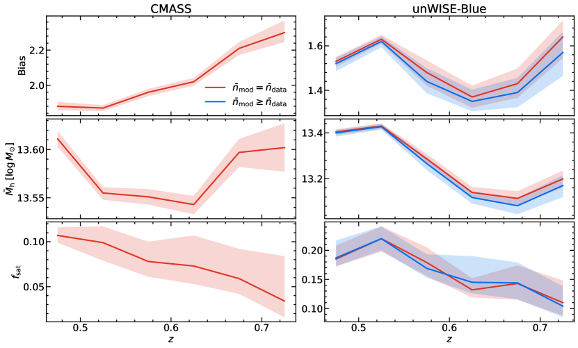
Figure 6: Evolution of the derived bias, mean halo mass ($\bar{M}_{h})$, and satellite fraction ($f_{\mathrm{sat}}$), parameters for the CMASS (left column) and unWISE-Blue (right column) galaxies as a function of redshift. The unWISE-Blue panels show both the default case where we use the observed $\bar{n}$ in the likelihood, and the “incompleteness” case where the model is allowed to have higher number density than the data (corresponding to a situation where the unWISE-Blue galaxies randomly down-sample best-fit HOD). The shaded regions represent the $\pm 1\sigma$ uncertainties derived from the MCMC samples.

5.1 CMASS

5.1.1 Redshift evolution of the CMASS HOD

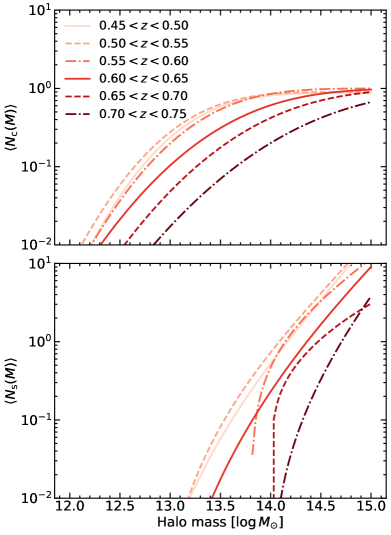
Figure 7: The mean number of central galaxies (top panel) and the mean number of satellite galaxies (bottom panel) for the CMASS HOD as functions of halo mass over all redshift bins. Note the evolution of in both $\langle N_{\mathrm{c}}(M)\rangle$ and $\langle N_{\mathrm{s}}(M)\rangle$ as a function of redshift. The sharp cutoff in $\langle N_{\mathrm{s}}(M)\rangle$ for $0.55<z<0.60$ and $0.60<z<0.65$ is due to the larger values of $\log_{10}(M_{0}/M_{\odot})$ (the mass at which there are zero satellite galaxies) for these bins, 13.8 and 14.0 respectively.

For CMASS, $M_{\textrm{min}}$ and $\sigma_{\log{M}}$ both significantly increase with redshift. This leads to an evolving HOD, i.e. the best-fit CMASS HOD in a single bin cannot fit the data in any other bin (holding the unWISE-Blue HOD constant). The evolving $N(M)$ is shown in Fig. 7. Despite the varying HOD parameters, the mean halo mass is constant from $0.5<z<0.65$ at $\log_{10}(M_{\mathrm{h}}/M_{\odot})\sim 13.55$, with a slight (but statistically significant) increase at $z>0.65$, and a similarly small decrease in the first redshift bin. This is due to a cancellation between the changes to $\langle N(M)\rangle$ (which favor higher halo mass at higher redshift) and the halo mass function, which exponentially decreases at the high mass end toward higher redshift. A halo of fixed mass is more biased at higher redshift, causing the mean halo bias to increase with redshift. The increase in $M_{\textrm{min}}$ and $\sigma_{\log{M}}$ also decreases the number density by decreasing $\langle N(M)\rangle$. Within the errorbars, $b(z)D(z)$ is quite close to constant at $z<0.65$ (ranging from 1.42 to 1.47) but then rises to 1.56 and 1.62 in the last two redshift bins. Finally, the satellite fraction declines with increasing redshift, but the changes are not statistically significant; the satellite fraction is $10^{+1.8}_{-1.7}\%$ in the $0.5<z<0.55$ bin.

5.1.2 Comparison to past work

These results for the CMASS HOD are similar to past findings. White et al. (2011) fit an HOD model to the correlation function measured from 44,000 CMASS galaxies at $0.4<z<0.7$ observed in the first semester of BOSS. Measuring within a single broad redshift bin at $z_{\textrm{eff}}=0.57$, they find $M_{\textrm{min}}=13.08\pm 0.12$, $M_{1}=14.06\pm 0.10$, $\sigma_{\log{M}}=0.60\pm 0.15$, $\alpha=0.90\pm 0.19$, and $M_{0}=13.13\pm 0.16$. These results are similar to our results in the $0.5<z<0.55$ and $0.55<z<0.6$ bin, though with a lower $M_{\textrm{min}}$ and $\sigma_{\log{M}}$. They find a mean halo mass of $M_{180b}=13.45\pm 0.03$ (equivalently 13.43 in our units, $M_{200b}$) and satellite fraction of $10\pm 2$%. Similarly, fitting to the DR10 projected correlation function and number density, Alam et al. (2017) finds best-fit values of $M_{\textrm{min}}=13.25$, $M_{1}=14.18$, $\sigma_{\log{M}}=0.54$, $M_{0}=12.39$, $\alpha=1.151$ (friends-of-friends halo masses). This yields a satellite fraction of 10% and a mean halo mass of 13.55 ($M_{200b}$). These parameters are in good agreement with our results except for the slightly lower $\sigma_{\log{M}}$. Reid et al. (2014) performs a similar fit, also including the monopole and quadrupole and varying the cosmological parameter $f\sigma_{8}$. They find $M_{\textrm{min}}=13.03\pm 0.03$, $\sigma_{\log M}=0.38\pm 0.06$, $M_{0}=13.27\pm 0.13$, $M_{1}=14.08\pm 0.06$, and $\alpha=0.76\pm 0.18$, for a satellite fraction of $10.2\pm 0.7$%, and a mean halo mass of 13.52.

Going beyond HOD measurements in a single redshift bin, Saito et al. (2016) fit the projected correlation function (across the entire redshift range) and the stellar mass function in narrow redshift bins to create mock catalogs that match the CMASS $n(z)$ and contain a redshift-evolving HOD. We compare our results to their publicly-available subhalo abundance-matched (SHAM) mock catalogs in Fig. 8. While both approaches find a redshift-evolving HOD, they are quite different in that Saito et al. (2016) only fit to the clustering in a single bin and use the stellar mass function to determine the redshift evolution, whereas we fit to the clustering in narrow redshift bins. Despite these differences, our HODs are qualitatively consistent in shape – i.e. $N_{\mathrm{c}}(M)$ and $N_{\mathrm{s}}(M)$ match well. However, Saito et al. (2016) finds a strong evolution in mean halo mass, from $\log_{10}(M_{\mathrm{h}}/M_{\odot})$ = 13.12 at $z=0.445$ to 13.66 at $z=0.685$, driven by the strong evolution in mean stellar mass. In contrast, we find a nearly constant mean halo mass. Saito et al. (2016) notes that their SHAM is inconsistent with the redshift-space monopole and quadrupole measured across the entire CMASS redshift range. Their model predicts a strong redshift evolution in the clustering amplitude of the multipoles (due to the strong increase in mean halo mass), which is not observed: the data is nearly constant in redshift (i.e. $b(z)D(z)$ is nearly constant). In contrast, our model is fit to the redshift-dependent clustering, and hence it shows much less evolution in mean halo mass and $b(z)D(z)$. Our results agree better with Saito et al. (2016) in the satellite fraction: they find a drop in the satellite fraction from 12% to 7% between $z=0.5$ and 0.7, matching our drop from 10% to 6%.

CMASS bin	$M_{\textrm{min}}$	$M_{1}$	$\alpha$	$M_{0}$	$\sigma_{\log{M}}$
$0.45<z<0.50$	$13.28^{+0.040}_{-0.041}$ (13.29)	$14.10^{+0.024}_{-0.034}$ (14.11)	$1.50^{+0.077}_{-0.091}$ (1.54)	$12.5^{+0.46}_{-0.36}$ (12.1)	$0.67^{+0.047}_{-0.054}$ (0.67)
$0.50<z<0.55$	$13.26^{+0.039}_{-0.037}$ (13.25)	$14.03^{+0.045}_{-0.093}$ (14.01)	$1.39^{+0.115}_{-0.152}$ (1.37)	$12.9^{+0.60}_{-0.59}$ (13.2)	$0.70^{+0.041}_{-0.040}$ (0.69)
$0.55<z<0.60$	$13.48^{+0.045}_{-0.038}$ (13.45)	$14.10^{+0.067}_{-0.181}$ (13.84)	$1.28^{+0.186}_{-0.274}$ (0.94)	$13.2^{+0.54}_{-0.80}$ (13.8)	$0.78^{+0.042}_{-0.036}$ (0.75)
$0.60<z<0.65$	$13.84^{+0.059}_{-0.047}$ (13.82)	$14.22^{+0.068}_{-0.129}$ (14.27)	$1.11^{+0.285}_{-0.287}$ (1.34)	$13.0^{+0.69}_{-0.66}$ (13.0)	$0.93^{+0.042}_{-0.036}$ (0.92)
$0.65<z<0.70$	$14.17^{+0.069}_{-0.062}$ (14.14)	$14.27^{+0.124}_{-0.299}$ (14.00)	$0.77^{+0.467}_{-0.457}$ (0.56)	$13.7^{+0.35}_{-1.05}$ (14.0)	$0.99^{+0.046}_{-0.045}$ (0.97)
$0.70<z<0.75$	$14.69^{+0.114}_{-0.106}$ (14.65)	$14.54^{+0.159}_{-0.317}$ (14.41)	$0.98^{+0.853}_{-0.634}$ (1.39)	$13.5^{+0.73}_{-1.01}$ (14.0)	$1.13^{+0.063}_{-0.068}$ (1.11)
Derived parameters	Bias	$\bar{M_{\mathrm{h}}}$ ($\log{M_{\odot}}$)	$f_{\textrm{sat}}$	$\chi^{2}$
$0.45<z<0.50$	$1.88^{+0.025}_{-0.022}$ (1.88)	$13.611^{+0.008}_{-0.008}$ (13.611)	$0.107^{+0.009}_{-0.009}$ (0.110)	16.155
$0.50<z<0.55$	$1.87^{+0.017}_{-0.018}$ (1.87)	$13.555^{+0.006}_{-0.007}$ (13.555)	$0.099^{+0.018}_{-0.020}$ (0.091)	14.498
$0.55<z<0.60$	$1.96^{+0.019}_{-0.021}$ (1.97)	$13.551^{+0.008}_{-0.008}$ (13.556)	$0.078^{+0.022}_{-0.017}$ (0.059)	6.675
$0.60<z<0.65$	$2.02^{+0.022}_{-0.022}$ (2.02)	$13.543^{+0.009}_{-0.010}$ (13.547)	$0.073^{+0.034}_{-0.020}$ (0.069)	9.033
$0.65<z<0.70$	$2.21^{+0.036}_{-0.037}$ (2.22)	$13.597^{+0.014}_{-0.015}$ (13.602)	$0.059^{+0.033}_{-0.017}$ (0.046)	9.012
$0.70<z<0.75$	$2.30^{+0.069}_{-0.054}$ (2.31)	$13.602^{+0.025}_{-0.025}$ (13.610)	$0.034^{+0.050}_{-0.018}$ (0.021)	5.772

Table 2: Marginalized and best-fit parameters for CMASS galaxies, requiring unWISE-Blue HOD to match observed number density. $\chi^{2}$ is the combined $\chi^{2}$ for the entire data vector (9 degrees of freedom).

unWISE-Blue bin	$M_{\textrm{min}}$	$M_{1}$	$\alpha$	$M_{0}$	$\sigma_{\log{M}}$
$0.45<z<0.50$	$12.20^{+0.083}_{-0.051}$ (12.16)	$13.16^{+0.137}_{-0.208}$ (13.09)	$1.11^{+0.132}_{-0.153}$ (1.06)	$12.9^{+0.27}_{-0.51}$ (13.0)	$0.23^{+0.213}_{-0.141}$ (0.07)
$0.50<z<0.55$	$12.28^{+0.062}_{-0.048}$ (12.24)	$13.33^{+0.049}_{-0.097}$ (13.30)	$1.30^{+0.046}_{-0.104}$ (1.28)	$12.2^{+0.50}_{-0.48}$ (12.4)	$0.22^{+0.161}_{-0.107}$ (0.15)
$0.55<z<0.60$	$12.66^{+0.244}_{-0.206}$ (12.73)	$13.35^{+0.069}_{-0.165}$ (13.27)	$1.19^{+0.073}_{-0.166}$ (1.10)	$12.4^{+0.52}_{-0.52}$ (12.8)	$0.87^{+0.217}_{-0.227}$ (0.96)
$0.60<z<0.65$	$12.99^{+0.238}_{-0.213}$ (13.00)	$13.23^{+0.181}_{-0.260}$ (13.11)	$0.89^{+0.177}_{-0.177}$ (0.82)	$13.0^{+0.23}_{-0.41}$ (13.1)	$1.15^{+0.162}_{-0.173}$ (1.18)
$0.65<z<0.70$	$12.90^{+0.260}_{-0.238}$ (12.95)	$13.50^{+0.064}_{-0.087}$ (13.51)	$1.15^{+0.089}_{-0.119}$ (1.16)	$12.2^{+0.55}_{-0.47}$ (11.7)	$1.04^{+0.195}_{-0.219}$ (1.08)
$0.70<z<0.75$	$12.53^{+0.281}_{-0.175}$ (12.39)	$13.38^{+0.152}_{-0.486}$ (12.47)	$1.14^{+0.219}_{-0.366}$ (0.62)	$13.0^{+0.43}_{-0.87}$ (13.6)	$0.61^{+0.309}_{-0.362}$ (0.38)
Derived parameters	Bias	$\bar{M_{\mathrm{h}}}$ ($\log{M_{\odot}}$)	$f_{\textrm{sat}}$
$0.45<z<0.50$	$1.53^{+0.020}_{-0.025}$ (1.54)	$13.404^{+0.012}_{-0.013}$ (13.407)	$0.185^{+0.023}_{-0.013}$ (0.180)
$0.50<z<0.55$	$1.63^{+0.019}_{-0.020}$ (1.63)	$13.430^{+0.011}_{-0.012}$ (13.430)	$0.220^{+0.021}_{-0.022}$ (0.216)
$0.55<z<0.60$	$1.48^{+0.054}_{-0.059}$ (1.45)	$13.286^{+0.022}_{-0.023}$ (13.273)	$0.179^{+0.026}_{-0.023}$ (0.164)
$0.60<z<0.65$	$1.37^{+0.051}_{-0.048}$ (1.35)	$13.140^{+0.024}_{-0.023}$ (13.131)	$0.132^{+0.020}_{-0.013}$ (0.127)
$0.65<z<0.70$	$1.43^{+0.068}_{-0.064}$ (1.41)	$13.114^{+0.031}_{-0.030}$ (13.104)	$0.143^{+0.031}_{-0.028}$ (0.184)
$0.70<z<0.75$	$1.64^{+0.074}_{-0.095}$ (1.69)	$13.199^{+0.036}_{-0.037}$ (13.223)	$0.110^{+0.038}_{-0.022}$ (0.088)

Table 3: Marginalized and best-fit parameters for unWISE galaxies, requiring unWISE-Blue HOD to match observed number density. $\chi^{2}$ is not shown, as Table 2 shows the combined $\chi^{2}$.

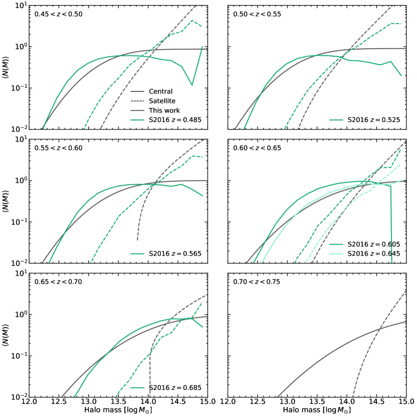
Figure 8: Comparison between our best-fit $\langle N(m)\rangle$ to the CMASS galaxies (gray lines) and those of Saito et al. (2016) (S2016; green lines). The solid lines depict $\langle N_{\mathrm{c}}(m)\rangle$ while the dashed lines depict $\langle N_{\mathrm{s}}(m)\rangle$. The S2016 measurements are reported in different redshift bins from our measurements, so we choose the nearest redshift bin to the center of each, reporting their central redshift value in each panel and comparing two bins from S2016 to our $0.6<z<0.65$ measurement. Note the qualitative similarities between the results in this paper and those in S2016 despite quantitative differences in methodology.

5.2 unWISE-Blue

5.2.1 Redshift evolution of the unWISE-Blue HOD—baseline results

Like CMASS, the unWISE-Blue sample HOD also evolves with redshift. If we require the model to match the unWISE number density (i.e. not allowing for incompleteness in $\langle N_{\mathrm{c}}(M)\rangle$), the largest difference is the dramatic increase of $M_{\textrm{min}}$ and $\sigma_{\log{M}}$ from the $0.5<z<0.55$ bin to $z>0.55$. This leads to a considerably different $\langle N_{\textrm{c}}(M)\rangle$ at $0.5<z<0.55$ than in the higher redshift bins (Fig. 9). We note that $M_{\textrm{min}}$ and $\sigma_{\log{M}}$ are strongly degenerate; while the 1D posteriors are very far apart on both parameters comparing $0.50<z<0.55$ and $0.55<z<0.60$, the 2D posteriors in the $M_{\textrm{min}}$–$\sigma_{\log{M}}$ plane just barely touch.

As with CMASS, we find that the best-fit HOD from the other redshift bins is strongly ruled out by the data in any redshift bin. We find that the average halo mass and bias generally decreases with redshift for the unWISE samples, with $\log_{10}(M_{\mathrm{h}}/M_{\odot})$ dropping from 13.4 at $z\sim 0.5$ to 13.1 at $z\sim 0.65$, and the bias dropping from 1.6 to 1.4 over the same redshift range. This is in contrast to the rough fit of Krolewski et al. (2020), who find $b(z)=0.8+1.2z$, implying an increase from $b=1.43$ to $b=1.61$ from $z=0.5$ to 0.7. However, that fitting function was a very approximate fit to underlying bias measurements that also decreased across the redshift range considered here of $0.45<z<0.75$, from 1.75 to 1.68 to 1.59 to 1.58 (dip in left panel of Fig. 19 in Krolewski et al. (2020)). The overall increasing $b(z)$ was intended to match the behavior over a much wider redshift range, $0<z<1$. Compared to CMASS, the unWISE galaxies have lower halo mass ($\log_{10}(M_{\mathrm{h}}/M_{\odot})$ $\sim 13.25$ vs. 13.55) and higher satellite fraction (15–20% vs. 6–10%).

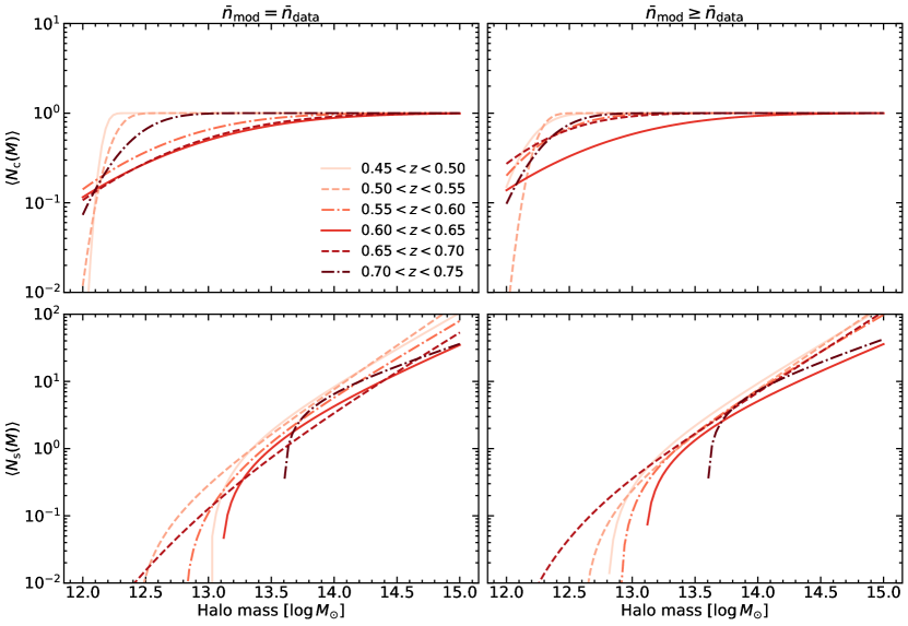
Figure 9: The mean number of central galaxies (top row) and the mean number of satellite galaxies (bottom row) for the unWISE-Blue HOD as functions of halo mass. The left column corresponds to the default case where we use the observed value of $\bar{n}$, while the right column corresponds to the “incompleteness” case where the model is allowed to have a higher $\bar{n}$ than the data. Plotting all redshift bins demonstrates the evolution of the unWISE-Blue HOD as a function of redshift. As in Fig. 7, the sharp drops in $\langle N_{\mathrm{s}}(M)\rangle$ occurr when the halo mass drops below $M_{0}$.

5.2.2 Allowing for incompleteness in unWISE-Blue

Tables 4 and 5 show our results if we allow for arbitrary incompleteness in the unWISE-Blue HOD. The unWISE-Blue HOD parameters are affected most strongly at $z>0.55$. This is because the clustering information alone favors an HOD matching the observed $\bar{n}(z)$ in the first two bins, whereas it prefers a larger $\bar{n}(z)$ at higher redshift. That is, the best-fit $f_{\textrm{inc}}$ is around 1 in the first two bins, but drops to around 0.5 at higher redshift. The most notable change at higher-$z$ is therefore a shift along the $M_{\textrm{min}}$–$\sigma_{\log{M}}$ degeneracy towards lower values of $M_{\textrm{min}}$ and higher number density. This shift is apparent in Fig. 9: $N_{\textrm{c}}$ with arbitrary incompleteness extends to lower halo mass, with a very slightly steeper dropoff, though not nearly as sharp as $N_{\textrm{c}}$ in the first two redshift bins.

When allowing for unWISE incompleteness, the CMASS parameters do not shift much, though the uncertainties are somewhat larger. The derived parameters are more stable to this change: the CMASS bias and mean halo mass (and their uncertainties) are nearly unchanged, and the median satellite fraction is similar but with somewhat larger errorbars. Likewise, the unWISE-Blue HODs have small changes in bias, mean halo mass, and satellite fraction, but these changes are all within the errorbar.

5.2.3 Comparison to past work

Kusiak et al. (2022) performs a similar analysis to us, fitting an HOD to the small-scale unWISE angular auto-correlation ($C_{\ell}^{gg}$) and cross-correlation with CMB lensing ($C_{\ell}^{\kappa g}$). Unlike this work, their HOD is redshift-independent, as they do not perform a tomographic measurement but rather consider only the galaxy auto-correlation and the cross-correlation with the broad CMB lensing kernel, neither of which allow them to extract redshift information. They also use a slightly different HOD model, fixing $M_{0}$ to zero and allowing the NFW truncation radius to vary as a free parameter.

For the unWISE-Blue sample, they find $\log_{10}(M_{\textrm{min}}/M_{\odot})=12.11\pm 0.37$, somewhat lower than our values. They also find a lower value for $M_{1}$, a slightly higher value for $\alpha$, and $\sigma_{\log{M}}=0.73^{+0.33}_{-0.22}$. Their derived parameters are quite consistent with ours, with a mean halo mass of $\log_{10}(M_{\mathrm{h}}/M_{\odot})=13.26\pm 0.02$, $b=1.50^{+0.01}_{-0.02}$, and satellite fraction of $0.23^{+0.06}_{-0.07}$. Our results suggest that while this redshift-independent HOD can fit the clustering of the entire unWISE-Blue sample well, a redshift-evolving HOD (with similar parameters on average) better fits the tomographic cross-correlation with CMASS spectroscopic galaxies. Our approach allows for dramatically improved resolution on the redshift evolution of the unWISE-Blue HOD, with better redshift resolution than previous work on different samples (i.e. the $\Delta z\sim 0.15$ photometric redshift bins in the DES redMaGiC and MagLim HOD analysis of Zacharegkas et al. (2022)).

6 Conclusions

We have measured the small-scale cross-correlation between the unWISE-Blue galaxies, selected via an infrared color cut from WISE imaging and possessing a broad redshift distribution at $0<z<1$, with the BOSS CMASS spectroscopic sample in narrow redshift bins of width $\Delta z=0.05$ between $z=0.45$ and 0.75. This allowed us to tomographically probe the unWISE and CMASS halo occupation distribution. We augmented the halo model, modifying the HALOMOD code (Murray et al., 2021), with the tools necessary to model this cross-correlation, including redshift-space distortions, beyond-Limber corrections, and halo exclusion. Our model fits the CMASS-unWISE cross-correlation and CMASS autocorrelation well at $0.1<r_{p}<10$ $h^{-1}$ Mpc.

We find that the CMASS HOD evolves strongly at $0.45<z<0.75$, with $\log_{10}(M_{\textrm{min}}/M_{\odot})$ increasing from 13.28 to 14.67 and the scatter $\sigma_{\log{M}}$ increasing from 0.67 to 1.11. The strong evolution in the halo mass function opposes the change in the HOD to yield a mean halo mass that is nearly constant, around $\log_{10}(M_{\mathrm{h}}/M_{\odot})=13.55$. The mean bias increases significantly, from 1.88 at $z=0.475$ to 2.32 at $z=0.725$. These results are largely consistent with past results, which generally fit the clustering of the sample across the entire redshift range (White et al., 2011; Reid et al., 2014; Saito et al., 2016; Alam et al., 2017).

The unWISE-Blue HOD is more constant than the CMASS HOD, and the evolution of the HOD parameters depends on whether we assume the HOD is complete at high masses, or allow for $\langle N_{c}(M)\rangle$ to asymptote to a value less than one at high halo masses. The evolution of derived parameters (mean bias, mean halo mass, and satellite fraction) is similar regardless of whether we allow for high-mass incompleteness. The bias is much more constant for unWISE-Blue than for CMASS; indeed, it declines only from $\sim$1.6 to $\sim$1.4 between $z\sim 0.5$ and 0.7. Likewise, the mean halo mass declines slightly from $\log_{10}(M_{\mathrm{h}}/M_{\odot}\sim 13.4$ to $\sim$13.1 from $z=0.5$ to 0.7. The satellite fraction of $\sim$20% is higher than the satellite fraction in BOSS, and declines slightly towards higher redshift.

The tomographic measurement of the unWISE-Blue HOD complements the previous unWISE-Blue HOD measurement of Kusiak et al. (2022) from the angular auto-correlation and the CMB lensing cross-correlation. Our HODs broadly agree with those of Kusiak et al. (2022), but our approach has the ability to test whether the HOD is redshift-independent, and indeed favors a modest evolution at $0.45<z<0.75$, spanning the peak of the unWISE-Blue redshift distribution. This distinction is potentially significant given the broad redshift distribution, and its implications for the unWISE auto-correlation and CMB lensing cross-correlation will be explored in future work. Our tomographic HOD model will also be useful for constructing mock catalogs for the unWISE-Blue sample (which are essential for cosmological modelling (Krolewski et al., 2021; Farren et al., 2024)) and for further enabling the use of this sample in cross-correlation measurements.

Code Availability

The code used to fit the data is available at https://github.com/jensenlawrence/CMASS-WISE-HOD.

Here we present additional tables and plots. In Tables 4 and 5, we give the marginalized constraints on the HOD and derived parameters for both CMASS and unWISE-Blue, allowing the unWISE-Blue model number density to exceed the data number density (i.e. allowing for an arbitrary $f_{\textrm{inc}}$ by removing the unWISE-Blue number density from the likelihood). In Figs. 10 and 11, we show contour plots for both the HOD and derived parameters for a representative redshift bin, $0.55<z<0.6$.

CMASS bin	$M_{\textrm{min}}$	$M_{1}$	$\alpha$	$M_{0}$	$\sigma_{\log{M}}$
$0.45<z<0.50$	$13.28^{+0.038}_{-0.039}$ (13.29)	$14.10^{+0.023}_{-0.030}$ (14.11)	$1.49^{+0.072}_{-0.081}$ (1.54)	$12.5^{+0.42}_{-0.36}$ (12.1)	$0.67^{+0.045}_{-0.050}$ (0.68)
$0.50<z<0.55$	$13.26^{+0.042}_{-0.038}$ (13.23)	$14.02^{+0.048}_{-0.079}$ (13.99)	$1.37^{+0.119}_{-0.131}$ (1.36)	$12.9^{+0.50}_{-0.60}$ (13.4)	$0.70^{+0.043}_{-0.041}$ (0.66)
$0.55<z<0.60$	$13.46^{+0.046}_{-0.037}$ (13.43)	$13.96^{+0.181}_{-0.310}$ (13.23)	$1.07^{+0.303}_{-0.356}$ (0.49)	$13.7^{+0.24}_{-0.77}$ (14.0)	$0.76^{+0.042}_{-0.038}$ (0.73)
$0.60<z<0.65$	$13.86^{+0.064}_{-0.051}$ (13.83)	$14.23^{+0.066}_{-0.084}$ (14.25)	$1.13^{+0.278}_{-0.274}$ (1.23)	$12.8^{+0.67}_{-0.52}$ (13.0)	$0.94^{+0.043}_{-0.038}$ (0.92)
$0.65<z<0.70$	$14.16^{+0.066}_{-0.058}$ (14.14)	$14.19^{+0.193}_{-0.828}$ (13.77)	$0.66^{+0.567}_{-0.463}$ (0.33)	$13.8^{+0.30}_{-1.09}$ (14.1)	$0.98^{+0.043}_{-0.042}$ (0.97)
$0.70<z<0.75$	$14.63^{+0.091}_{-0.087}$ (14.63)	$12.78^{+0.503}_{-0.372}$ (12.61)	$0.24^{+0.295}_{-0.177}$ (0.32)	$14.4^{+0.22}_{-0.19}$ (14.6)	$1.10^{+0.057}_{-0.058}$ (1.10)
Derived parameters	Bias	$\bar{M_{\mathrm{h}}}$ ($\log{M_{\odot}}$)	$f_{\textrm{sat}}$	$\chi^{2}$
$0.45<z<0.50$	$1.88^{+0.021}_{-0.021}$ (1.88)	$13.610^{+0.008}_{-0.007}$ (13.610)	$0.108^{+0.009}_{-0.009}$ (0.110)	16.403
$0.50<z<0.55$	$1.87^{+0.016}_{-0.017}$ (1.88)	$13.555^{+0.006}_{-0.006}$ (13.558)	$0.098^{+0.020}_{-0.018}$ (0.083)	14.372
$0.55<z<0.60$	$1.96^{+0.021}_{-0.021}$ (1.96)	$13.551^{+0.009}_{-0.008}$ (13.549)	$0.064^{+0.022}_{-0.011}$ (0.052)	6.651
$0.60<z<0.65$	$2.02^{+0.020}_{-0.023}$ (2.03)	$13.542^{+0.009}_{-0.009}$ (13.547)	$0.081^{+0.037}_{-0.022}$ (0.074)	9.089
$0.65<z<0.70$	$2.21^{+0.035}_{-0.034}$ (2.22)	$13.597^{+0.014}_{-0.014}$ (13.599)	$0.053^{+0.029}_{-0.017}$ (0.044)	9.042
$0.70<z<0.75$	$2.31^{+0.066}_{-0.055}$ (2.30)	$13.604^{+0.024}_{-0.023}$ (13.604)	$0.015^{+0.012}_{-0.008}$ (0.012)	5.730

Table 4: As in Table 2, but for the case where the model number density is allowed to exceed the observed number density.

unWISE-Blue bin	$M_{\textrm{min}}$	$M_{1}$	$\alpha$	$M_{0}$	$\sigma_{\log{M}}$
$0.45<z<0.50$	$12.19^{+0.093}_{-0.082}$ (12.19)	$13.14^{+0.147}_{-0.213}$ (13.10)	$1.11^{+0.138}_{-0.153}$ (1.06)	$12.8^{+0.28}_{-0.64}$ (13.0)	$0.26^{+0.210}_{-0.168}$ (0.22)
$0.50<z<0.55$	$12.26^{+0.066}_{-0.064}$ (12.24)	$13.31^{+0.059}_{-0.092}$ (13.28)	$1.30^{+0.049}_{-0.093}$ (1.25)	$12.3^{+0.44}_{-0.49}$ (12.6)	$0.21^{+0.160}_{-0.110}$ (0.13)
$0.55<z<0.60$	$12.38^{+0.287}_{-0.243}$ (12.32)	$13.11^{+0.200}_{-0.312}$ (13.17)	$1.10^{+0.115}_{-0.177}$ (1.09)	$12.7^{+0.34}_{-0.50}$ (12.9)	$0.75^{+0.195}_{-0.187}$ (0.54)
$0.60<z<0.65$	$12.40^{+0.481}_{-0.510}$ (12.84)	$12.98^{+0.268}_{-0.298}$ (13.00)	$0.98^{+0.144}_{-0.190}$ (0.78)	$12.8^{+0.34}_{-0.71}$ (13.1)	$0.87^{+0.283}_{-0.396}$ (1.09)
$0.65<z<0.70$	$12.29^{+0.529}_{-0.382}$ (12.30)	$13.20^{+0.235}_{-0.238}$ (13.30)	$1.15^{+0.088}_{-0.117}$ (1.20)	$12.3^{+0.53}_{-0.51}$ (12.0)	$0.73^{+0.352}_{-0.334}$ (0.70)
$0.70<z<0.75$	$12.34^{+0.265}_{-0.256}$ (12.33)	$13.10^{+0.280}_{-0.431}$ (12.44)	$1.05^{+0.227}_{-0.273}$ (0.64)	$13.1^{+0.34}_{-0.62}$ (13.6)	$0.49^{+0.342}_{-0.309}$ (0.36)
Derived parameters	Bias	$\bar{M_{\mathrm{h}}}$ ($\log{M_{\odot}}$)	$f_{\textrm{sat}}$	$f_{\textrm{inc}}$
$0.45<z<0.50$	$1.52^{+0.026}_{-0.034}$ (1.54)	$13.400^{+0.013}_{-0.016}$ (13.408)	$0.187^{+0.030}_{-0.014}$ (0.180)	$0.830^{+0.154}_{-0.083}$ (0.874)
$0.50<z<0.55$	$1.62^{+0.022}_{-0.026}$ (1.63)	$13.427^{+0.012}_{-0.013}$ (13.430)	$0.220^{+0.021}_{-0.020}$ (0.208)	$0.949^{+0.132}_{-0.091}$ (0.960)
$0.55<z<0.60$	$1.44^{+0.059}_{-0.053}$ (1.52)	$13.266^{+0.028}_{-0.028}$ (13.299)	$0.169^{+0.024}_{-0.016}$ (0.157)	$0.480^{+0.241}_{-0.127}$ (0.563)
$0.60<z<0.65$	$1.35^{+0.053}_{-0.044}$ (1.36)	$13.118^{+0.026}_{-0.026}$ (13.126)	$0.145^{+0.045}_{-0.019}$ (0.126)	$0.478^{+0.394}_{-0.177}$ (0.780)
$0.65<z<0.70$	$1.39^{+0.066}_{-0.066}$ (1.42)	$13.082^{+0.033}_{-0.037}$ (13.094)	$0.144^{+0.035}_{-0.028}$ (0.155)	$0.619^{+0.445}_{-0.252}$ (0.648)
$0.70<z<0.75$	$1.57^{+0.093}_{-0.105}$ (1.67)	$13.170^{+0.045}_{-0.050}$ (13.212)	$0.104^{+0.034}_{-0.019}$ (0.091)	$0.738^{+0.423}_{-0.195}$ (0.895)

Table 5: As in Table 3, but for the case where the model number density is allowed to exceed the observed number density.

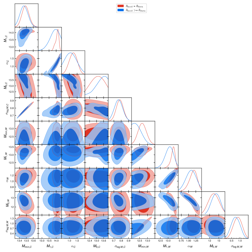
Figure 10: Constraints and degeneracies between the 10 HOD parameters at $0.55<z<0.6$. A subscript $C$ denotes the CMASS HOD parameters while a subscript $W$ denotes the unWISE-Blue HOD parameters. The default model is in red, and the model allowing for unWISE incompleteness is in blue. Parameter degeneracies are similar in other redshift bins.

References

- Aihara et al. (2011) Aihara, H., Allende Prieto, C., An, D., et al. 2011, ApJS, 193, 29
- Alam et al. (2017) Alam, S., Miyatake, H., More, S., Ho, S., & Mandelbaum, R. 2017, MNRAS, 465, 4853
- Asgari et al. (2023) Asgari, M., Mead, A. J., & Heymans, C. 2023, The Open Journal of Astrophysics, 6, 39
- Berlind et al. (2003) Berlind, A. A., Weinberg, D. H., Benson, A. J., et al. 2003, ApJ, 593, 1
- Beutler et al. (2013) Beutler, F., Blake, C., Colless, M., et al. 2013, MNRAS, 429, 3604
- Bloch & Johnson (2024) Bloch, R. & Johnson, M. C. 2024, arXiv e-prints, arXiv:2405.00809
- Bundy et al. (2015) Bundy, K., Leauthaud, A., Saito, S., et al. 2015, ApJS, 221, 15
- Coil (2013) Coil, A. L. 2013, in Planets, Stars and Stellar Systems. Volume 6: Extragalactic Astronomy and Cosmology, ed. T. D. Oswalt & W. C. Keel, Vol. 6, 387
- Cooray & Sheth (2002) Cooray, A. & Sheth, R. 2002, Phys. Rep., 372, 1
- Davis & Peebles (1983) Davis, M. & Peebles, P. J. E. 1983, ApJ, 267, 465
- Dawson et al. (2013) Dawson, K. S., Schlegel, D. J., Ahn, C. P., et al. 2013, AJ, 145, 10
- Dodelson & Schneider (2013) Dodelson, S. & Schneider, M. D. 2013, Phys. Rev. D, 88, 063537
- Doi et al. (2010) Doi, M., Tanaka, M., Fukugita, M., et al. 2010, AJ, 139, 1628
- Duffy et al. (2008) Duffy, A. R., Schaye, J., Kay, S. T., & Dalla Vecchia, C. 2008, MNRAS, 390, L64
- Eisenstein et al. (2011) Eisenstein, D. J., Weinberg, D. H., Agol, E., et al. 2011, AJ, 142, 72
- Farren et al. (2024) Farren, G. S., Krolewski, A., MacCrann, N., et al. 2024, ApJ, 966, 157
- Farren et al. (2023) Farren, G. S., Sherwin, B. D., Bolliet, B., et al. 2023, arXiv e-prints, arXiv:2311.04213
- Favole et al. (2016) Favole, G., McBride, C. K., Eisenstein, D. J., et al. 2016, MNRAS, 462, 2218
- Fukugita et al. (1996) Fukugita, M., Ichikawa, T., Gunn, J. E., et al. 1996, AJ, 111, 1748
- Gaia Collaboration et al. (2018) Gaia Collaboration, Brown, A. G. A., Vallenari, A., et al. 2018, A&A, 616, A1
- Górski et al. (2005) Górski, K. M., Hivon, E., Banday, A. J., et al. 2005, ApJ, 622, 759
- Gunn et al. (1998) Gunn, J. E., Carr, M., Rockosi, C., et al. 1998, AJ, 116, 3040
- Gunn et al. (2006) Gunn, J. E., Siegmund, W. A., Mannery, E. J., et al. 2006, AJ, 131, 2332
- Guo et al. (2013) Guo, H., Zehavi, I., Zheng, Z., et al. 2013, ApJ, 767, 122
- Guo et al. (2014) Guo, H., Zheng, Z., Zehavi, I., et al. 2014, MNRAS, 441, 2398
- Hartlap et al. (2007) Hartlap, J., Simon, P., & Schneider, P. 2007, A&A, 464, 399
- Howlett et al. (2012) Howlett, C., Lewis, A., Hall, A., & Challinor, A. 2012, J. Cosmology Astropart. Phys, 1204, 027
- Kaiser (1987) Kaiser, N. 1987, MNRAS, 227, 1
- Krause et al. (2013) Krause, E., Hirata, C. M., Martin, C., Neill, J. D., & Wyder, T. K. 2013, MNRAS, 428, 2548
- Krolewski & Ferraro (2022) Krolewski, A. & Ferraro, S. 2022, J. Cosmology Astropart. Phys, 2022, 033
- Krolewski et al. (2020) Krolewski, A., Ferraro, S., Schlafly, E. F., & White, M. 2020, J. Cosmology Astropart. Phys, 2020, 047
- Krolewski et al. (2021) Krolewski, A., Ferraro, S., & White, M. 2021, Journal of Cosmology and Astroparticle Physics, 2021 [\eprint[arXiv]2105.03421]
- Kusiak et al. (2021) Kusiak, A., Bolliet, B., Ferraro, S., Hill, J. C., & Krolewski, A. 2021, Phys. Rev. D, 104, 043518
- Kusiak et al. (2022) Kusiak, A., Bolliet, B., Krolewski, A., & Hill, J. C. 2022, Phys. Rev. D, 106, 123517
- Laigle et al. (2016) Laigle, C., McCracken, H. J., Ilbert, O., et al. 2016, ApJS, 224, 24
- Lang (2014) Lang, D. 2014, AJ, 147, 108
- Leauthaud et al. (2016) Leauthaud, A., Bundy, K., Saito, S., et al. 2016, MNRAS, 457, 4021
- Lewis et al. (2000) Lewis, A., Challinor, A., & Lasenby, A. 2000, ApJ, 538, 473
- Limber (1953) Limber, D. N. 1953, ApJ, 117, 134
- Lupton et al. (2001) Lupton, R., Gunn, J. E., Ivezić, Z., Knapp, G. R., & Kent, S. 2001, in Astronomical Society of the Pacific Conference Series, Vol. 238, Astronomical Data Analysis Software and Systems X, ed. J. Harnden, F. R., F. A. Primini, & H. E. Payne, 269
- Ma & Fry (2000) Ma, C.-P. & Fry, J. N. 2000, ApJ, 543, 503
- Mainzer et al. (2014) Mainzer, A., Bauer, J., Cutri, R. M., et al. 2014, ApJ, 792, 30
- Mainzer et al. (2011) Mainzer, A., Bauer, J., Grav, T., et al. 2011, ApJ, 731, 53
- McQuinn & White (2013) McQuinn, M. & White, M. 2013, MNRAS, 433, 2857
- Mead et al. (2021) Mead, A. J., Brieden, S., Tröster, T., & Heymans, C. 2021, MNRAS, 502, 1401
- Meisner et al. (2017) Meisner, A. M., Lang, D., & Schlegel, D. J. 2017, AJ, 153, 38
- Ménard et al. (2013) Ménard, B., Scranton, R., Schmidt, S., et al. 2013, arXiv e-prints, arXiv:1303.4722
- Miyaji et al. (2011) Miyaji, T., Krumpe, M., Coil, A. L., & Aceves, H. 2011, ApJ, 726, 83
- Mohammad & Percival (2022) Mohammad, F. G. & Percival, W. J. 2022, MNRAS, 514, 1289
- Murray et al. (2021) Murray, S., Diemer, B., Chen, Z., et al. 2021, Astronomy and Computing, 36, 100487
- Myers et al. (2005) Myers, A. D., Outram, P. J., Shanks, T., et al. 2005, MNRAS, 359, 741
- Navarro et al. (1997) Navarro, J. F., Frenk, C. S., & White, S. D. M. 1997, ApJ, 490, 493
- Newman (2008) Newman, J. A. 2008, ApJ, 684, 88
- Ouellette & Holder (2024) Ouellette, A. & Holder, G. 2024, arXiv e-prints, arXiv:2405.09633
- Padmanabhan et al. (2008) Padmanabhan, N., Schlegel, D. J., Finkbeiner, D. P., et al. 2008, ApJ, 674, 1217
- Peacock & Smith (2000) Peacock, J. A. & Smith, R. E. 2000, MNRAS, 318, 1144
- Percival et al. (2022) Percival, W. J., Friedrich, O., Sellentin, E., & Heavens, A. 2022, MNRAS, 510, 3207
- Percival et al. (2014) Percival, W. J., Ross, A. J., Sánchez, A. G., et al. 2014, MNRAS, 439, 2531
- Pier et al. (2003) Pier, J. R., Munn, J. A., Hindsley, R. B., et al. 2003, AJ, 125, 1559
- Planck Collaboration et al. (2016) Planck Collaboration, Ade, P. A. R., Aghanim, N., et al. 2016, A&A, 594, A13
- Reid et al. (2016) Reid, B., Ho, S., Padmanabhan, N., et al. 2016, MNRAS, 455, 1553
- Reid et al. (2014) Reid, B. A., Seo, H.-J., Leauthaud, A., Tinker, J. L., & White, M. 2014, MNRAS, 444, 476
- Roche & Eales (1999) Roche, N. & Eales, S. A. 1999, MNRAS, 307, 703
- Rocher et al. (2023) Rocher, A., Ruhlmann-Kleider, V., Burtin, E., et al. 2023, arXiv e-prints, arXiv:2306.06319
- Saito et al. (2016) Saito, S., Leauthaud, A., Hearin, A. P., et al. 2016, MNRAS, 460, 1457
- Schlafly et al. (2019) Schlafly, E. F., Meisner, A. M., & Green, G. M. 2019, ApJS, 240, 30
- Seljak (2000) Seljak, U. 2000, MNRAS, 318, 203
- Sellentin & Heavens (2016) Sellentin, E. & Heavens, A. F. 2016, MNRAS, 456, L132
- Simon (2007) Simon, P. 2007, A&A, 473, 711
- Smee et al. (2013) Smee, S. A., Gunn, J. E., Uomoto, A., et al. 2013, AJ, 146, 32
- Smith et al. (2002) Smith, J. A., Tucker, D. L., Kent, S., et al. 2002, AJ, 123, 2121
- Smith et al. (2002) Smith, R. E., Peacock, J. A., Jenkins, A., et al. 2002, Monthly Notices of the Royal Astronomical Society, 341, 1311
- Takahashi et al. (2012) Takahashi, R., Sato, M., Nishimichi, T., Taruya, A., & Oguri, M. 2012, Astrophysical Journal, 761
- Tinker et al. (2008) Tinker, J., Kravtsov, A. V., Klypin, A., et al. 2008, ApJ, 688, 709
- Tinker et al. (2017) Tinker, J. L., Brownstein, J. R., Guo, H., et al. 2017, ApJ, 839, 121
- Tinker et al. (2010) Tinker, J. L., Robertson, B. E., Kravtsov, A. V., et al. 2010, ApJ, 724, 878
- Tinker et al. (2005) Tinker, J. L., Weinberg, D. H., Zheng, Z., & Zehavi, I. 2005, ApJ, 631, 41
- Torrado & Lewis (2021) Torrado, J. & Lewis, A. 2021, J. Cosmology Astropart. Phys, 2021, 057
- Wenzl et al. (2023) Wenzl, L., Chen, S.-F., & Bean, R. 2023, arXiv e-prints, arXiv:2308.05892
- White et al. (2011) White, M., Blanton, M., Bolton, A., et al. 2011, ApJ, 728, 126
- Wright et al. (2010) Wright, E. L., Eisenhardt, P. R. M., Mainzer, A. K., et al. 2010, AJ, 140, 1868
- Yan et al. (2024) Yan, Z., Maniyar, A. S., & van Waerbeke, L. 2024, J. Cosmology Astropart. Phys, 2024, 058
- York et al. (2000) York, D. G., Adelman, J., Anderson, Jr., J. E., et al. 2000, AJ, 120, 1579
- Yuan et al. (2020) Yuan, S., Eisenstein, D. J., & Leauthaud, A. 2020, MNRAS, 493, 5551
- Yuan et al. (2022) Yuan, S., Garrison, L. H., Hadzhiyska, B., Bose, S., & Eisenstein, D. J. 2022, MNRAS, 510, 3301
- Yuan et al. (2021) Yuan, S., Hadzhiyska, B., Bose, S., Eisenstein, D. J., & Guo, H. 2021, MNRAS, 502, 3582
- Zacharegkas et al. (2022) Zacharegkas, G., Chang, C., Prat, J., et al. 2022, MNRAS, 509, 3119
- Zehavi et al. (2005) Zehavi, I., Zheng, Z., Weinberg, D. H., et al. 2005, ApJ, 630, 1
- Zhai et al. (2023) Zhai, Z., Percival, W. J., & Guo, H. 2023, MNRAS, 523, 5538
- Zhai et al. (2017) Zhai, Z., Tinker, J. L., Hahn, C., et al. 2017, ApJ, 848, 76
- Zheng et al. (2007) Zheng, Z., Coil, A. L., & Zehavi, I. 2007, ApJ, 667, 760
- Zhou et al. (2023) Zhou, R., Ferraro, S., White, M., et al. 2023, J. Cosmology Astropart. Phys, 2023, 097