Estimating Optimal Dynamic Treatment Regimes Using Irregularly Observed Data: A Target Trial Emulation and Bayesian Joint Modeling Approach

Abstract

An optimal dynamic treatment regime (DTR) is a sequence of decision rules aimed at providing the best course of treatments individualized to patients. While conventional DTR estimation uses longitudinal data, such data can also be irregular, where patient-level variables can affect visit times, treatment assignments and outcomes. In this work, we first extend the target trial framework – a paradigm to estimate statistical estimands specified under hypothetical randomized trials using observational data – to the DTR context; this extension allows treatment regimes to be defined with intervenable visit times. We propose an adapted version of G-computation marginalizing over random effects for rewards that encapsulate a treatment strategy’s value. To estimate components of the G-computation formula, we then articulate a Bayesian joint model to handle correlated random effects between the outcome, visit and treatment processes. We show via simulation studies that, in the estimation of regime rewards, failure to account for the observational treatment and visit processes produces bias which can be removed through joint modeling. We also apply our proposed method on data from INSPIRE 2 and 3 studies to estimate optimal injection cycles of Interleukin 7 to treat HIV-infected individuals.

Keywords: Adaptive treatment strategies, informative visit times, G-computation, correlated random effects

toc

1 Introduction

A dynamic treatment regime (DTR), also known as an adaptive treatment strategy, is a sequence of deterministic decision rules which, at every stage, assigns a treatment given an individual’s available history (Murphy, 2003; Moodie et al., 2007). In particular, interest lies in estimating the optimal DTR, which maximizes a quantity that can comprise of long-term and short-term outcomes (Murphy, 2003). In the context of precision medicine, these regimes allow decision-makers to tailor treatments with respect to a patient’s evolving health status and response to their previous treatments.

Sequential Multiple Assignment Randomized Trials (SMART) are study designs in which participants are randomized at every stage of a treatment sequence (Lavori and Dawson, 2000; Lei et al., 2012). SMARTs are ideal for developing DTRs but such trials are often impractical in practice due to logistical, ethical, and financial constraints (Wallace et al., 2016). As a result, researchers often rely on observational data to infer causal estimands and optimal DTRs (Lavori and Dawson, 2000; Lei et al., 2012). G-computation and marginal structural models (MSMs) have been used to estimate causal quantities with observational data, accounting for time-varying confounders (Hernán and Robins, 2020; Robins, 2000). However, observational longitudinal data can also be subject to irregular observation times, which can introduce bias if not properly accounted for (Zeger and Liang, 1986; Pullenayegum and Lim, 2016). Methods to account for irregularly observed data are generally built on generalized estimating equations (GEE) or joint modeling (Pullenayegum and Lim, 2016; Gasparini et al., 2020). In the former, bias induced by informative visit times can be corrected using inverse intensity weights (IIW). In the Bayesian paradigm, but not limited to it, methods for accounting for irregularly observed data have relied on shared or correlated random effects by jointly modeling the outcome and visit processes (Farewell et al., 2017; Ryu et al., 2007).

Bayesian methods have increasingly been applied to the estimation of DTRs, offering flexible frameworks to account for time-varying confounders and the complexities of longitudinal data. These approaches include two-step quasi-Bayesian methods, Bayesian extensions of MSMs, and techniques that utilize inverse probability treatment weighting (IPTW) within a Bayesian framework (Hoshino, 2008; Keil et al., 2018; Saarela et al., 2015). Recent advances have focused on estimating optimal DTRs, mainly using Bayesian methods, tailored for irregularly observed data (Coulombe et al., 2023; Guan et al., 2020; Hua et al., 2022; Oganisian et al., 2024). However, despite such recent methodological developments, there is limited work on using Bayesian joint models with correlated random effects with irregularly observed data to estimate optimal DTRs with intervenable visit times. One way to address this methodological problem is to build on the framework of the target trial, a hypothetical randomized trial whose purpose is to define causal quantities of interest such that they can be estimated using observational data (Hernán, 2011; Hernán and Robins, 2016). The DTR estimation problem has usually been formulated in the potential outcomes framework. Alternatively, the DTR estimation problem based on observational, possibly irregular, longitudinal data could be framed with respect to an ideal SMART by extending the target trial emulation framework. However, it appears that this has not been fully explored in the literature. In our work, we address these gaps by introducing a new yet parsimonious target trial notation and we show how optimal DTRs can be estimated using Bayesian joint modeling when sub-processes affect each other.

2 Methods

2.1 Notation

Akin to Yiu et al. (2022), we begin by simultaneously using the target trial paradigm from Hernán and Robins (2016) and the mathematical notation from Dawid and Didelez (2010)’s decision-theoretic framework. The target trial concept provides a formal causal framework that allowing explicit definition of each component of the trial under which we wish to define our causal estimand of interest (Hernán and Robins, 2016; Hernán et al., 2022). We then extend these frameworks by incorporating visit times information into both the target trial concept and the decision-theoretic mathematical notation.

We denote outcomes $Y_{ij}$, covariates $X_{ij}$ with $W_{ij}=(Y_{ij},X_{ij})$, treatments $A_{ij}$ and visit times $T_{ij}$ where $j\in\mathbb{N}$ indexes the observation number of an individual $i\in\mathbb{N}$. We denote $U_{i}=(U_{i,\mathrm{Y}},U_{i,\mathrm{X}},U_{i,\mathrm{A}},U_{i,\mathrm{T}})$ to be individual-specific random effects corresponding to each process and $\zeta_{i}$ to be the right-censoring time. Hereon, unless we talk about estimation procedures, we omit that subscript $i$ for notational simplicity, with all defined variables understood to be specific to any individual $i\in\mathbb{N}$. The overbar notation, e.g. $\overline{t}_{j}=(t_{1},\dots,t_{j})$, denotes a set of accrued variables and the underline notation, e.g. $\underline{t}_{j}=(t_{j},\dots,t_{K+1})$, represents accrued future variables; without loss of generality, we assume that $\overline{t}_{0}=\emptyset$ and the same for other variables. DTRs consist of decision functions $d_{j}$ where the corresponding treatment $d_{j}(h_{j})=a_{j}\in\Psi_{j}(h_{j})$ is assigned according to the history $h_{j}=(\overline{t}_{j},\overline{w}_{j},\overline{a}_{j-1})$ among possible options $\Psi_{j}(h_{j})$, also referred as the feasible set (Tsiatis et al., 2019). Furthermore, we define the optimal midstream DTR $\underline{d}_{k}^{\text{opt}}=\big{(}d^{\text{opt}}_{k},\dots,d_{K}^{\text{opt}}\big{)}$ maximizing a reward conditional on past history $H_{k}=h_{k}$. Optimal stage $j$ decisions $d_{j}^{\text{opt}}$ are defined recursively assuming that future decisions $d_{j+1}^{\text{opt}},\dots,d_{K}^{\text{opt}}$ are optimal.

2.2 Target Trial Definition

We define $\mathcal{R}_{k}(h_{k},\underline{t}_{k+1},\underline{d}_{k},\phi_{\mathcal{R}})$ as the reward which, conditional on past history $H_{k}=h_{k}$, is a function of expected outcomes from stages $k+1$ to $K+1$; we use $\phi_{\mathcal{R}}$ to represent reward parameters which we will expand in Section 2.3:

$$\mathcal{R}_{k}(h_{k},\underline{t}_{k+1},\underline{d}_{k},\phi_{\mathcal{R}}) =\sum_{j=k+1}^{K+1}\gamma_{j}\mathbb{E}_{\mathcal{E}}\left[Y_{j}\mid\overline{T}_{j}=\overline{t}_{j},\overline{A}_{j-1}=\overline{d}_{j-1},\overline{W}_{k}=\overline{w}_{k},\phi_{\mathcal{R}}\right]\,,$$

for any $i\in\mathbb{N}$. The conditional statement $A_{j}=d_{j}$ means that the random variable $A_{j}$ is assigned the treatment value of $d_{j}(h_{j})$ and $\overline{A}_{j-1}=\overline{d}_{j-1}$ means that the first $k-1$ treatments $\overline{a}_{k-1}\subset h_{k}$ are conditioned on and future treatments $a_{k},\dots,a_{j}$ are assigned according to the decision rules $d_{k},\dots,d_{j}$. Notice that $\mathcal{R}_{k}(h_{k},\underline{t}_{k+1},\underline{d}_{k},\phi_{\mathcal{R}})$ is marginal over $W_{k+1},\dots,W_{K+1}$ but are conditional on $\overline{W}_{k}=\overline{w}_{k}\subset h_{k}$. With the reward defined under $\mathcal{E}$ given $\phi_{\mathcal{R}}$, $d_{j}^{\text{opt}}$ can be defined recursively through backwards induction where we are primarily interested in the optimal decision function under true parameters $\phi_{\mathcal{R}0}$, i.e. $d_{j}^{\text{opt}}(h_{j},\phi_{\mathcal{R}0})$:

$$d_{j}^{\text{opt}}(h_{j},\phi_{\mathcal{R}}) =\operatorname*{argmax}_{a_{j}\in\Psi_{j}(h_{j})}\,\mathcal{R}_{j}\Big{(}h_{j},\underline{t}_{j+1},\big{(}a_{j},\underline{d}_{j+1}^{\text{opt}}\big{)},\phi_{\mathcal{R}}\Big{)}\quad\text{for }j=k,\dots,K-1\,,$$

with $d_{K}^{\text{opt}}(h_{K},\phi_{\mathcal{R}})=\operatorname*{argmax}_{a_{K}\in\Psi_{K}(h_{K})}\,\mathcal{R}_{K}\Big{(}h_{K},t_{K+1},\overline{a}_{K},\phi_{\mathcal{R}}\Big{)}$ being the terminal case. We expand on the recursive nature of $d_{j}^{\text{opt}}$’s in Appendix A.

 

Figure 1: Left: DAG for the observational ($\mathcal{O}$) data-generating process where three visits occur before censoring time. Right: DAG representing the target trial model ($\mathcal{E}$) of a two-stage regime in which treatments and observation times are no longer driven by past covariates, outcomes and latent random effects. Both DAGs encode the assumption that the random effects $U=(U_{\mathrm{W}},U_{\mathrm{A}},U_{\mathrm{T}})$ are independent conditional on $U^{*}$, a latent factor that affects them.

We model $\mathcal{E}$ as a SMART trial for estimating optimal DTRs, assuming that treatments $A_{j+1}$ and observation times $T_{j+1}$ are randomized independently of individual-specific information Lavori and Dawson (2000). Although randomization could incorporate individual characteristics and even be combined with deterministic decision rules, we focus here on a completely randomized SMART as our $\mathcal{E}$ for simplicity:

$$\overline{W}_{j+1},U\perp\!\!\!\perp_{\mathcal{E}}T_{j+1}\mid\overline{T}_{j},\overline{A}_{j},\phi_{\mathrm{T}}^{*}\,\,\,\text{and}\,\,\,\overline{W}_{j},U\perp\!\!\!\perp_{\mathcal{E}}A_{j}\mid\overline{T}_{j},\overline{A}_{j-1},\phi_{\mathrm{A}}^{*}\,,\quad\text{for }j=1,\dots,K\,,$$

where $\phi_{\mathrm{T}}^{*},\phi_{\mathrm{A}}^{*}$ are parameters respectively driving the target trial visit and treatment assignment processes. Equivalently, these conditions can be specified in $\mathcal{E}-$densities:

$$f_{\mathcal{E}}(a_{j+1},t_{j+1}\mid\overline{w}_{j+1},\overline{a}_{j},\overline{t}_{j},u,\phi_{\mathrm{A}}^{*},\phi_{\mathrm{T}}^{*})=f_{\mathcal{E}}(a_{j+1},t_{j+1}\mid\overline{a}_{j},\overline{t}_{j},\phi_{\mathrm{A}}^{*},\phi_{\mathrm{T}}^{*})\,,$$

for all $j=1,\dots,K-1$ and $f_{\mathcal{E}}(t_{K+1}\mid\overline{a}_{K},\overline{w}_{K},\overline{t}_{K},u,\phi_{\mathrm{T}}^{*})$ = $f_{\mathcal{E}}(t_{K+1}\mid\overline{a}_{K},\overline{t}_{K},\phi_{\mathrm{T}}^{*})$. Under these trial specifications, $\mathcal{R}_{k}(h_{k},\underline{t}_{k+1},\underline{d}_{k},\phi_{\mathcal{R}})$ can be written as follows:

$$\mathcal{R}_{k}(h_{k},\underline{t}_{k+1},\underline{d}_{k},\phi_{\mathcal{R}}) =\bigintsss_{u_{\mathrm{W}}}\left\{\sum_{j=k+1}^{K+1}\gamma_{j}\mathbb{E}_{\mathcal{E}}\left[Y_{j}\mid\overline{T}_{j}=\overline{t}_{j},\overline{A}_{j-1}=\overline{d}_{j-1},\overline{W}_{k}=\overline{w}_{k},u_{\mathrm{W}},\phi_{\mathrm{W}}\right]\right\}$$

$$\qquad\quad\times f_{\mathcal{E}}(u_{\mathrm{W}}\mid\overline{t}_{k},\overline{w}_{k},\overline{d}_{k-1},\phi_{\mathcal{R}})\,du_{\mathrm{W}}$$

$$=\bigintsss_{u_{\mathrm{W}}}\bigintsss_{w_{j+1}}\dots\bigintsss_{w_{K+1}}\sum_{j=k+1}^{K+1}\gamma_{j}y_{j}$$

$$\quad\times\frac{\left\{\prod_{j=k+1}^{K+1}f_{\mathcal{E}}(w_{j}\mid\overline{t}_{j},\overline{d}_{j-1},\overline{w}_{j-1},u_{\mathrm{W}},\phi_{\mathrm{W}})\right\}f_{\mathcal{E}}(u_{\mathrm{W}}\mid\phi_{\mathrm{U}})}{\bigintss_{u_{\mathrm{W}}}\left\{\prod_{j=1}^{k}f_{\mathcal{E}}(w_{j}\mid\overline{t}_{j},\overline{d}_{j-1},\overline{w}_{j-1},u_{\mathrm{W}},\phi_{\mathrm{W}})\right\}f_{\mathcal{E}}(u_{\mathrm{W}}\mid\phi_{\mathrm{U}})du_{\mathrm{W}}}$$

$$\quad\times dw_{K+1}\dots dw_{k+1}du_{\mathrm{W}}\,.$$

The full derivation is available in the Appendix B. While we consider $W_{j}$ as continuous variables, all integrals can be generalized by defining them as Riemann-Stieltjes integrals and cumulative distribution functions. By factorizing the rewards as above, we find that optimal rewards and regimes only depend on two sets of parameters, hence $\phi_{\mathcal{R}}=(\phi_{\mathrm{W}},\phi_{\mathrm{U}})$. The dotted arrows in Figure 1 linking random effects indicates their possible dependence. The absence of correlation between the random effects, reflecting unobserved individual-level variation, would render certain model components ignorable for outcomes. This would allow the likelihood to factorize into separate components and allowing inference to be carried out without modeling the treatment and visit processes (Farewell et al., 2017). In particular, in our work, we take interest in the scenario where this is not the case.

2.3 Relating the Target Trial and the Observational Setting

While data under $\mathcal{E}$ are unavailable, we can still infer on estimands defined under $\mathcal{E}$ using $\mathcal{O}$ data through several causal assumptions outlined in A1–A4.

1. Stability of random effects: the prior distribution of random effects $U_{\mathrm{W}}$ given $\phi_{\mathrm{U}}$ is the same under $\mathcal{E}$ and $\mathcal{O}$:

   $$f_{\mathcal{E}}(u_{\mathrm{W}}\mid\phi_{\mathrm{U}})=f_{\mathcal{O}}(u_{\mathrm{W}}\mid\phi_{\mathrm{U}})\,,$$

   for any $\phi_{\mathrm{U}}$.

1. Extended stability of observables:

   $$f_{\mathcal{E}}(w_{j}\mid\overline{t}_{j},\overline{a}_{j-1},\overline{w}_{j-1},u_{\mathrm{W}},\phi_{\mathrm{W}})=f_{\mathcal{O}}(w_{j}\mid\overline{t}_{j},\overline{a}_{j-1},\overline{w}_{j-1},u_{\mathrm{W}},\phi_{\mathrm{W}})\,,$$

   for $j=1,\dots,K+1$, for all $i\in\mathbb{N}$, for any $\phi_{\mathrm{W}}$.

1. Impact of random effects on longitudinal observations: Under $\mathcal{O}$, distributions of observables only depend on their corresponding random effects and parameters:

   $$T_{j}\perp\!\!\!\perp_{\mathcal{O}}U_{\mathrm{W}},U_{\mathrm{A}} \mid\overline{A}_{j-1},\overline{W}_{j-1},\overline{T}_{j-1},U_{\mathrm{T}},\phi_{\mathrm{T}}$$

   $$W_{j}\perp\!\!\!\perp_{\mathcal{E},\mathcal{O}}U_{\mathrm{T}},U_{\mathrm{A}} \mid\overline{T}_{j},\overline{A}_{j-1},\overline{W}_{j-1},U_{\mathrm{W}},\phi_{\mathrm{W}}$$

   $$A_{j}\perp\!\!\!\perp_{\mathcal{O}}U_{\mathrm{T}},U_{\mathrm{W}} \mid\overline{W}_{j-1},\overline{T}_{j-1},\overline{A}_{j-1},U_{\mathrm{A}},\phi_{\mathrm{A}}\,,$$

   for $j=1,\dots,K$. Recall that, from Section 2.2, the distributions of $A_{j}$ and $T_{j}$’s are defined as desired under $\mathcal{E}$. These assumptions complement the definition of the target trial from the previous subsection.

1. Positivity: conditional distributions under $\mathcal{E}$ of $A_{j}$ and $T_{j}$, given all past variables that could be observed, are absolutely continuous with respect to their $\mathcal{O}$ analogues:

   $$f_{\mathcal{E}}(a_{j}\mid\overline{t}_{j},\overline{a}_{j-1},\phi_{\mathrm{A}}^{*})>0 \Rightarrow f_{\mathcal{O}}\big{(}a_{j}\mid\overline{w}_{j},\overline{t}_{j},\overline{a}_{j-1},u_{\mathrm{A}},\phi_{\mathrm{A}})>0\,,\hskip 29.87547pt\text{for all $j=1,\dots,K$}\,;$$

   $$f_{\mathcal{E}}(t_{j}\mid\overline{a}_{j-1},\overline{t}_{j-1},\phi_{\mathrm{T}}^{*})>0 \Rightarrow f_{\mathcal{O}}\big{(}t_{j}\mid\overline{a}_{j-1},\overline{w}_{j-1},\overline{t}_{j-1},u_{i,\mathrm{T}},\phi_{\mathrm{T}})>0\,,\quad\text{for all $j=1,\dots,K+1$}\,,$$

   for all possible values of $u_{\mathrm{T}},u_{\mathrm{A}},\phi_{\mathrm{T}},\phi_{\mathrm{A}},\phi_{\mathrm{T}}^{*},\phi_{\mathrm{A}}^{*}$ and for all $i\in\mathbb{N}$.

Because stability assumptions A1 and A2 posit equivalencies in conditional distributions under $\mathcal{E}$ and $\mathcal{O}$, $\phi_{\mathrm{W}}$ parametrizes the conditional distribution of $W_{ij}$ under both $\mathcal{E}$ and $\mathcal{O}$ in A3. Moreover, these stability assumptions imply that the target trial and observational study have the same target population, i.e. same eligibility, inclusion and exclusion criteria. We provide an extended version of G-computation that builds upon Dawid and Didelez (2010) by tailoring their proposed causal assumptions to infer on our rewards as per Figure 1.

Theorem 1 (Extended G-Computation).

The conditional reward $\mathcal{R}_{k}(h_{k},\underline{t}_{k+1},\underline{d}_{k},\phi_{\mathcal{R}})$ can be expressed as an integral with respect to probability measures under $\mathcal{O}$ under A1–A4:

$$\mathcal{R}_{k}(h_{k},\underline{t}_{k+1},\underline{d}_{k},\phi_{\mathcal{R}}) =\bigintsss_{u_{\mathrm{W}}}\bigintsss_{w_{k+1}}\dots\bigintsss_{w_{K+1}}\sum_{j=k+1}^{K+1}\gamma_{j}y_{j}$$

$$\quad\times\frac{\left\{\prod_{j=1}^{K+1}f_{\mathcal{O}}(w_{j}\mid\overline{t}_{j},\overline{d}_{j-1},\overline{w}_{j-1},u_{i,\mathrm{W}},\phi_{\mathrm{W}})\right\}f_{\mathcal{O}}(u_{\mathrm{W}}\mid\phi_{\mathrm{U}})}{\bigintss_{u_{\mathrm{W}}}\left\{\prod_{j=1}^{k}f_{\mathcal{O}}(w_{j}\mid\overline{t}_{j},\overline{d}_{j-1},\overline{w}_{j-1},u_{\mathrm{W}},\phi_{\mathrm{W}})\right\}f_{\mathcal{O}}(u_{\mathrm{W}}\mid\phi_{\mathrm{U}})du_{\mathrm{W}}}$$

$$\quad\times\,dw_{K+1}\dots\,dw_{j+1}\,du_{\mathrm{W}}\,.$$

Proof.

The proof is available in the Appendix C. ∎

2.4 Bayesian Estimation: Parameters, Rewards and Optimal Decisions

We let $\pi_{0}(\phi)$ denote the prior on $\phi$ and $\pi_{n}(\phi)$ to denote the posterior distribution of $\phi$ given the data of $n$ observed individuals under $\mathcal{O}$. We are primarily interested in $\pi_{n}(\phi_{\mathcal{R}})=\int_{\phi_{\mathrm{T}},\phi_{\mathrm{A}}}\pi_{n}(d\phi)$, the marginal posterior distribution of $\phi_{\mathcal{R}}$, because they parametrize our rewards. Following Saarela et al. (2015), the proof that the reward evaluated at $\phi_{\mathcal{R}0}$ can be expressed as a limiting case of an integral with respect to the posterior $\pi_{n}(\phi_{\mathcal{R}})$ is available in Appendix D.1.

While the characterization of regimes, $\mathcal{E},\mathcal{O}$ processes and causal assumptions have been made entirely non-parametrically so far, model specifications are required to carry out posterior sampling. A pivotal point of this work stems from the requirement of $\pi_{n}(\phi_{\mathcal{R}})$ needing a joint model for fitting due to the presence of correlated random effects $U=(U_{\mathrm{W}},U_{\mathrm{A}},U_{\mathrm{T}})$ through its prior $f_{\mathcal{O}}(u\mid\phi_{\mathrm{U}})$. In other words, no components can be taken out of the integral to solely infer on the posterior $\pi_{n}(\phi_{\mathcal{R}})\stackrel{{\scriptstyle\phi_{\mathcal{R}}}}{{\propto}}\pi_{n}(\phi)$ which, in product form, is:

$$\pi_{n}(\phi) \propto\bigintsss_{u_{1},\dots,u_{n}}\Bigg{\{}\prod_{i=1}^{n}\Bigg{\{}\prod_{j=1}^{m_{i}}f_{\mathcal{O}}\big{(}w_{ij}\mid\overline{t}_{ij},\overline{a}_{i(j-1)},\overline{w}_{i(j-1)},u_{i,\mathrm{W}},\phi_{\mathrm{W}}\big{)}$$

$$\hskip 56.9055pt\times f_{\mathcal{O}}\big{(}t_{ij}\mid\overline{a}_{i(j-1)},\overline{w}_{i(j-1)},\overline{t}_{i(j-1)},u_{i,\mathrm{T}},\phi_{\mathrm{T}}\big{)}$$

$$\hskip 56.9055pt\times\mathbbm{1}_{j>1}\bigg{[}f_{\mathcal{O}}\big{(}a_{i(j-1)}\mid\overline{w}_{i(j-1)},\overline{t}_{i(j-1)},\overline{a}_{i(j-2)},u_{i,\mathrm{A}},\phi_{\mathrm{A}}\big{)}\bigg{]}\Bigg{\}}$$

$$\hskip 56.9055pt\times\left(1-\bigintsss_{t_{im_{i}}}^{\zeta_{i}}f_{\mathcal{O}}(s\mid\overline{w}_{im_{i}},\overline{t}_{im_{i}},\overline{a}_{i(m_{i}-1)},u_{i,\mathrm{T}},\phi_{\mathrm{T}})\,ds\right)f_{\mathcal{O}}(u_{i}\mid\phi_{\mathrm{U}})\Bigg{\}}\pi_{0}(\phi)\,.$$

The visit process contribution to likelihood formula above assumes an absence of competing risks, such as death, which is presumed to be a sufficiently rare outcome to be disregarded; this assumption is reasonable in the context of our data analysis in Section 4.

To estimate the optimal reward given $\phi_{\mathcal{R}}$, we simulate each treatment arm in a forward fashion. At each decision point $j\geqslant k$, the treatment arm yielding the maximum reward conditional the new simulated history $h_{j}$ serves as the optimal reward for the specific $\phi_{\mathcal{R}}$ value. To estimate the true conditional expectations $\mathbb{E}_{\mathcal{E}}\left[Y_{j}\mid\overline{T}_{j}=\overline{t}_{j},\overline{A}_{j-1}=\overline{d}_{j-1},\overline{W}_{k}=\overline{w}_{k},\phi_{\mathcal{R}}\right]$ in rewards, we carry out Monte Carlo integration for each posterior draw $\phi_{\mathcal{R}}^{(b)}$. With random effects $u_{\mathrm{W}}$ influenced by $h_{j}$ which is being conditioned on, a Metropolis algorithm is needed to sample from $f_{\mathcal{E}}(u_{\mathrm{W}}\mid\overline{w}_{k},\overline{t}_{k},\overline{d}_{k-1},\phi_{\mathrm{U}})$, which is the same distribution under $\mathcal{O}$ by Bayes’ Theorem and stability assumptions A1–A2. We provide details about the computational procedure in Appendix D.2. Given sufficiently large amounts of posterior draws via MCMC and Monte Carlo samples, the Monte Carlo error of posterior estimates should be negligible, i.e. converging to 0; see Appendix D.3 for more details.

3 Simulation Study

In our simulation study, we demonstrate that joint modeling of all model components ensures unbiased reward estimates, enabling more accurate identification and estimation of optimal treatment regimes.

3.1 Setup

We posit a data-generating process under $\mathcal{O}$ to estimate $\mathcal{E}$ quantities of interest, here rewards and optimal regimes. We begin by generating each individual’s unmeasured confounders $U_{i}=\log(U_{i,\mathrm{T}}),U_{i,\mathrm{W}},U_{i,\mathrm{A}}\mid\Sigma_{0}\sim\operatorname{MVN}\big{(}0,\Sigma_{0}\big{)}$ where $\Sigma_{0}$ specifies the degree of correlation between model-specific random effects. We define $\Sigma_{0}$ here to be a $3\times 3$ matrix with diagonal entries to be 0.36 and other correlation values to be 0.216. We simulate individual visits $T_{i1},\dots$ until the censoring time $\zeta_{i}\sim\operatorname{Unif}(3.5,4)$ is attained; each simulated individual has the observed data $\big{\{}(t_{ij},a_{ij},w_{ij})\big{\}}_{i=1}^{m_{i}}\cup\left\{t_{i(m_{i}+1)},w_{i(m_{i}+1)},m_{i}\right\}$ under $\mathcal{O}$. We define model-specific histories $H_{ij,\mathrm{A}}=\big{[}1,Y_{ij},X_{ij},A_{i(j-1)}\big{]}$, $H_{ij,\mathrm{Y}}=\big{[}1,T_{ij},X_{ij},A_{i(j-1)},A_{i(j-1)}X_{ij},A_{i(j-1)}T_{ij}\big{]}$ and $H_{ij,\mathrm{X}}=H_{ij,\mathrm{T}}=\big{[}X_{i(j-1)},A_{i(j-1)}\big{]}$. Under $\mathcal{O}$, at every time point $T_{ij}$, we simulate a corresponding “mark” $(W_{ij},A_{ij})$ given historic data according to the equations below and the following data-generating parameters: $\phi_{\mathrm{T}0}=(-0.3,0.5)$, $\lambda_{0}=0.2$, $\alpha_{0}=3.5$, $\phi_{\mathrm{Y}0}=(-0.3,0.3,0.3,0.55,-0.5,-0.5)$, $\phi_{\mathrm{A}0}=(0.2,-0.2,0.2)$, $\phi_{\mathrm{X}0}=(0.4,0.4)$ and $\tau_{\mathrm{X}0}^{2}=0.3$.

$$A_{ij}\mid\overline{W}_{ij},\overline{T}_{ij},\overline{A}_{i(j-1)},U_{i,\mathrm{A}},\phi_{\mathrm{A}} \sim\operatorname{Bern}\left(\Phi^{-1}\left(H_{ij,\mathrm{A}}^{\top}\phi_{\mathrm{A}}+U_{i,\mathrm{A}}\right)\right)$$

$$X_{ij}\mid\overline{T}_{ij},\overline{A}_{i(j-1)},\overline{W}_{i(j-1)},\phi_{\mathrm{X}} \sim\mathcal{N}\left(H_{ij,\mathrm{X}}^{\top}\phi_{\mathrm{X}}\scalebox{1.2}{,}\,\tau_{\mathrm{X}}^{2}\right)$$

$$Y_{ij}\mid\overline{X}_{ij},\overline{T}_{ij},\overline{A}_{i(j-1)},U_{i,\mathrm{Y}},\phi_{\mathrm{Y}} \sim\operatorname{Bern}\left(\Phi^{-1}\left(H_{ij,\mathrm{Y}}^{\top}\phi_{\mathrm{Y}}+U_{i,\mathrm{Y}}\right)\right)$$

$$T_{ij}-T_{i(j-1)}\mid\overline{W}_{i(j-1)},\overline{A}_{i(j-1)},\overline{T}_{i(j-1)},U_{i,\mathrm{T}},\phi_{\mathrm{T}} \sim\operatorname{Weibull}\left(\lambda_{0}\log(U_{i,\mathrm{T}})\exp\left\{H_{ij,\mathrm{T}}^{\top}\phi_{\mathrm{T}}\right\}\scalebox{1.2}{,}\,\alpha\right)$$

We provide the data-generating mechanism in Appendix E. Conditional on the posterior draw $\phi^{(b)}$, a posterior distribution of regime rewards can be obtained via Theorem 1. Using Monte Carlo integration for each $\phi^{(b)}$ as per Appendix D.2, we can estimate conditional rewards using an arbitrary large Monte Carlo sample size, i.e. $10\,000\,000$ here. Under $\mathcal{O}$, we simulate “training” sets of $n=100$ and $n=300$ participants whose data are used for posterior inference of $\phi_{\mathcal{R}}$. For each training set (or simulation replication), we carry out the Bayesian estimation procedure under four model specifications: $(Y,A,T)$, $(Y,A)$, $(Y,T)$ and $(Y)$. We refer to the latter three as “partial models” as at least one of the treatment and visit processes are not modeled. If included, they are all correctly specified; for instance, the outcome, time-varying covariate and treatment assignment processes are correctly specified in $(Y,A)$ but the visit process is not modeled at all.

Posterior draws of these parameters under each of the four models are used to estimate 1) the scalar-valued $\mathcal{R}_{k}(h_{k},\underline{t}_{k+1},\underline{d}_{k}^{\text{opt}},\phi_{\mathcal{R}0})$ and 2) the individualized treatments at visit times $t_{i2}=2$ and $t_{i3}=3$ for a “test” set of 100 participants not utilized in the posterior inference procedure for $\phi_{\mathcal{R}}$. Here, we define our feasible sets to be $\{0,1\}$ for all stages under $\mathcal{E}$. We carry out simulations for two sets of history profiles consisting of one observed visit: for $i=1$, $\overline{x}_{11}=x_{11}=-0.35$, $\overline{y}_{11}=y_{11}=1$ and, for $i=2$, $\overline{x}_{21}=x_{21}=0.35$, $\overline{y}_{21}=y_{21}=0$. We refer to these two patient histories as $h_{11}=(x_{11},y_{11})$ and $h_{21}=(x_{21},y_{21})$ respectively. For patient 1 with history $h_{11}$, $(d_{2}^{\text{opt}},d_{3}^{\text{opt}})=(1,d_{3}^{\text{opt}})$ with a true optimal reward value of 1.132 and, for patient 2 with history $h_{21}$, $(d_{2}^{\text{opt}},d_{3}^{\text{opt}})=(0,d_{3}^{\text{opt}})$ with a true optimal reward value of 0.952. The third treatment is left “to be decided” with respect to the decision function $d_{3}^{\text{opt}}$ according to their evolving status after their second visit:

$$\text{Patient 1:}\quad\max_{a\in\{0,1\}}\mathcal{R}_{1}\big{(}h_{11},(2,3),(a,d_{3}^{\text{opt}}),\phi_{\mathcal{R}0}\big{)} =\mathcal{R}_{1}\big{(}h_{11},(2,3),(1,d_{3}^{\text{opt}}),\phi_{\mathcal{R}0}\big{)}\approx 1.132\,;$$

$$\text{Patient 2:}\quad\max_{a\in\{0,1\}}\mathcal{R}_{1}\big{(}h_{11},(2,3),(a,d_{3}^{\text{opt}}),\phi_{\mathcal{R}0}\big{)} =\mathcal{R}_{1}\big{(}h_{21},(2,3),(0,d_{3}^{\text{opt}}),\phi_{\mathcal{R}0}\big{)}\approx 0.952\,.$$

We also simulate a “test” set of $n_{\text{test}}=100$ individuals from $\mathcal{E}$ and identify their optimal individualized treatments at times $2$ and $3$. We report the mean agreement rate (AR), the average probability of identifying the correct optimal treatment under all four model specifications across all $n_{\text{test}}$ individuals. Finally, generating $h_{i1}$ under $\mathcal{E}$ with $t_{1}=1$ and assuming future $t_{2}=2$ and $t_{3}=3$, we define individual-specific estimated benefit, bias and ARs for each test subject $i\in\{n+1,\dots,n+n_{\text{test}}\}$ as follows:

$$\operatorname{Benefit}_{i} =\mathcal{R}_{1}\big{(}h_{i1},(2,3),(1,d_{3}^{\text{opt}}),\phi_{\mathcal{R}0}\big{)}-\mathcal{R}_{1}\big{(}h_{i1},(2,3),(0,d_{3}^{\text{opt}}),\phi_{\mathcal{R}0}\big{)}$$

$$\operatorname{Bias}_{i} =\frac{1}{S}\sum_{s=1}^{S}\mathbb{E}_{\phi_{\mathcal{R}}\mid\mathcal{F}_{n}^{(s)}}\left[\mathcal{R}_{1}\big{(}h_{i1},(2,3),(\widehat{d}_{2}^{\text{opt}},\widehat{d}_{3}^{\text{opt}}),\phi_{\mathcal{R}}\big{)}\right]-\mathcal{R}_{1}\big{(}h_{i1},(2,3),(d_{2}^{\text{opt}},d_{3}^{\text{opt}}),\phi_{\mathcal{R}0}\big{)}$$

$$\operatorname{AR}_{i} =\frac{1}{S}\sum_{s=1}^{S}\mathbbm{1}\left\{\mathcal{R}_{1}\big{(}h_{i1},(2,3),(d_{2}^{\text{opt}},d_{3}^{\text{opt}}),\phi_{\mathcal{R}0}\big{)}=\mathbb{E}_{\phi_{\mathcal{R}}\mid\mathcal{F}_{n}^{(s)}}\left[\mathcal{R}_{1}\big{(}h_{i1},(2,3),(\widehat{d}_{2}^{\text{opt}},\widehat{d}_{3}^{\text{opt}}),\phi_{\mathcal{R}}\big{)}\right]\right\}\,.$$

We also elaborate on Monte Carlo error estimates across simulation replications in Appendix D.4.

3.2 Simulation Results

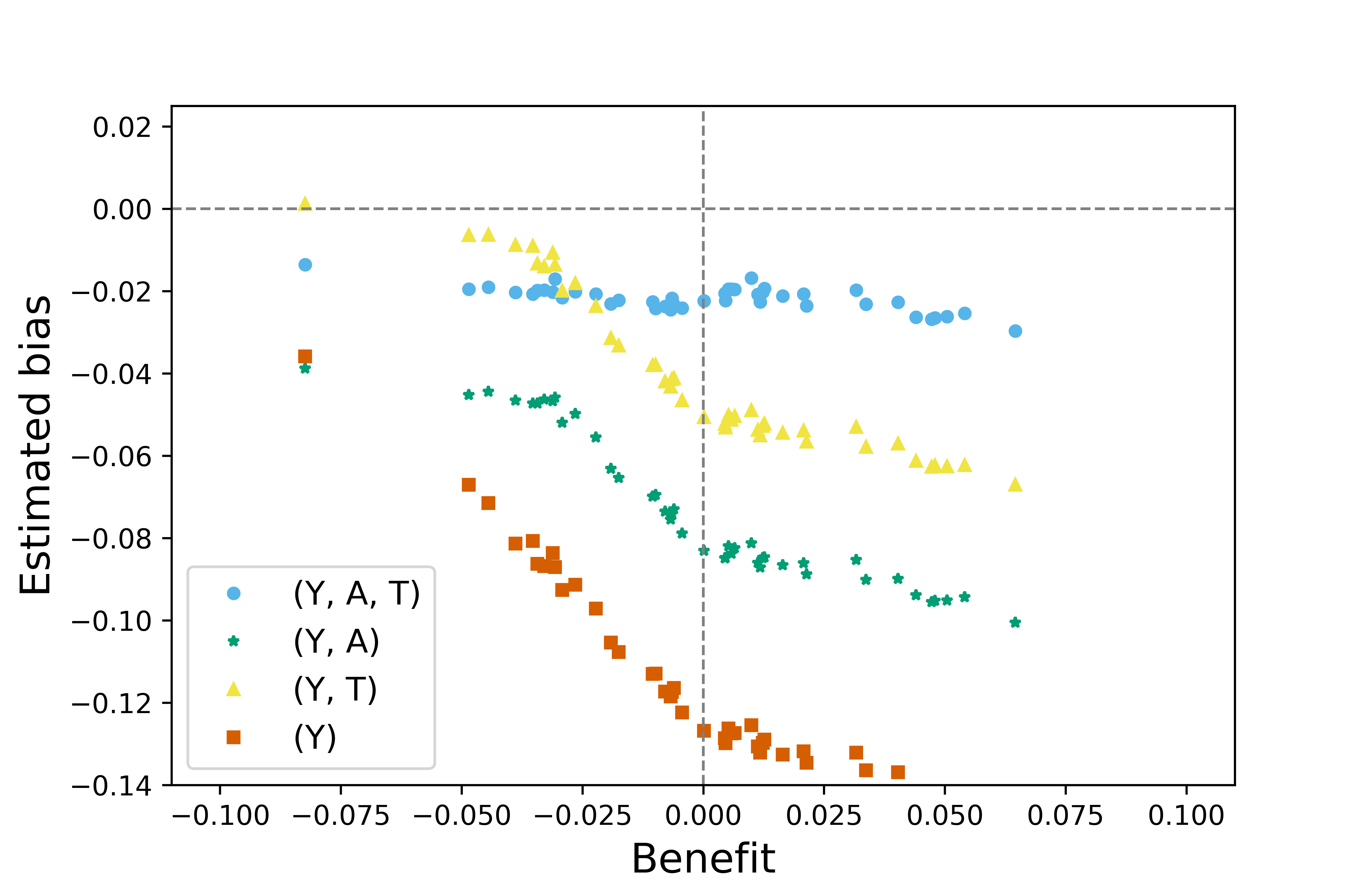
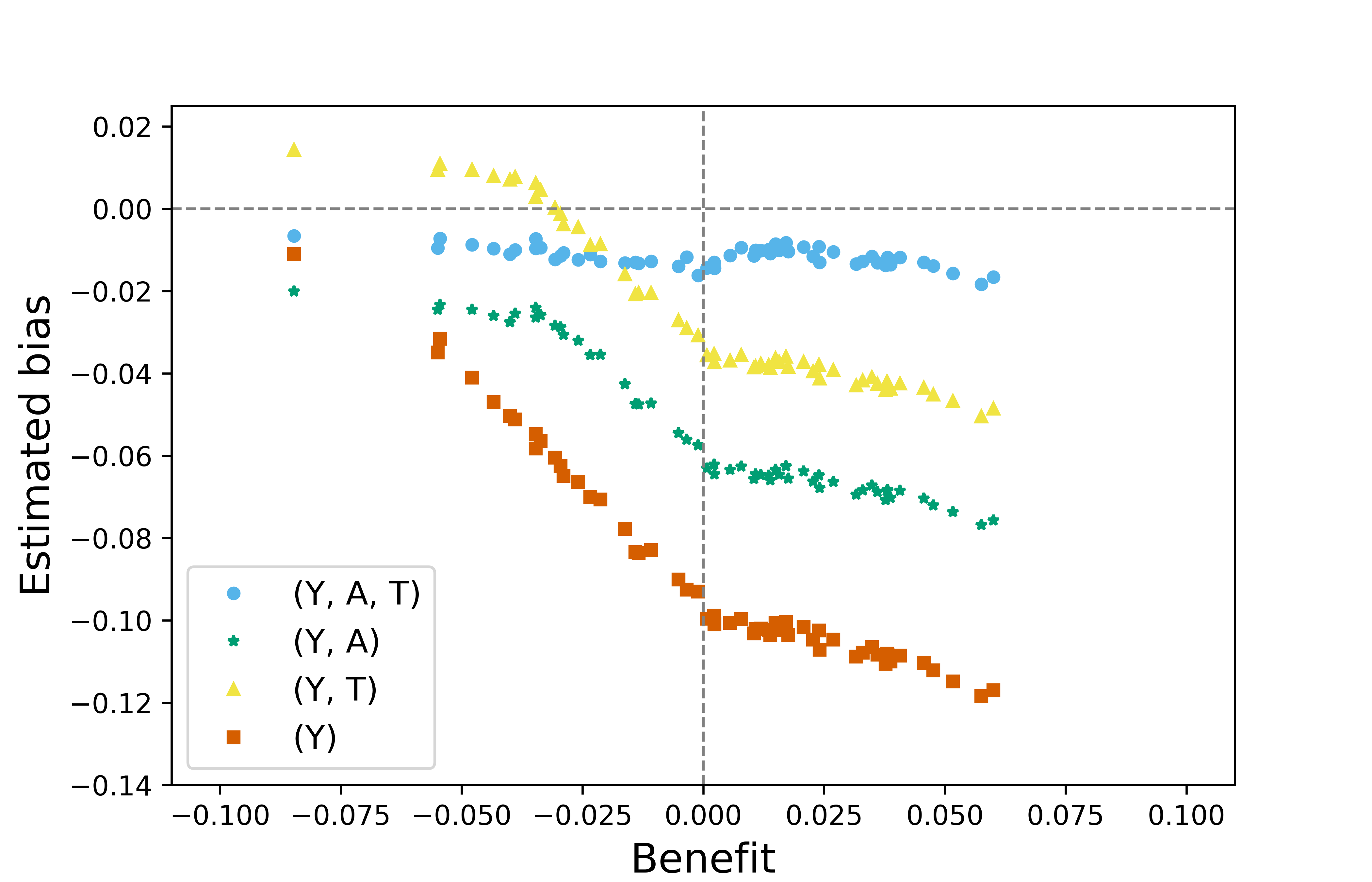
Figure 2: Benefit vs. estimated bias for all four model specifications given previous outcome $y_{i1}=0$ (left) and $y_{i1}=1$ (right).

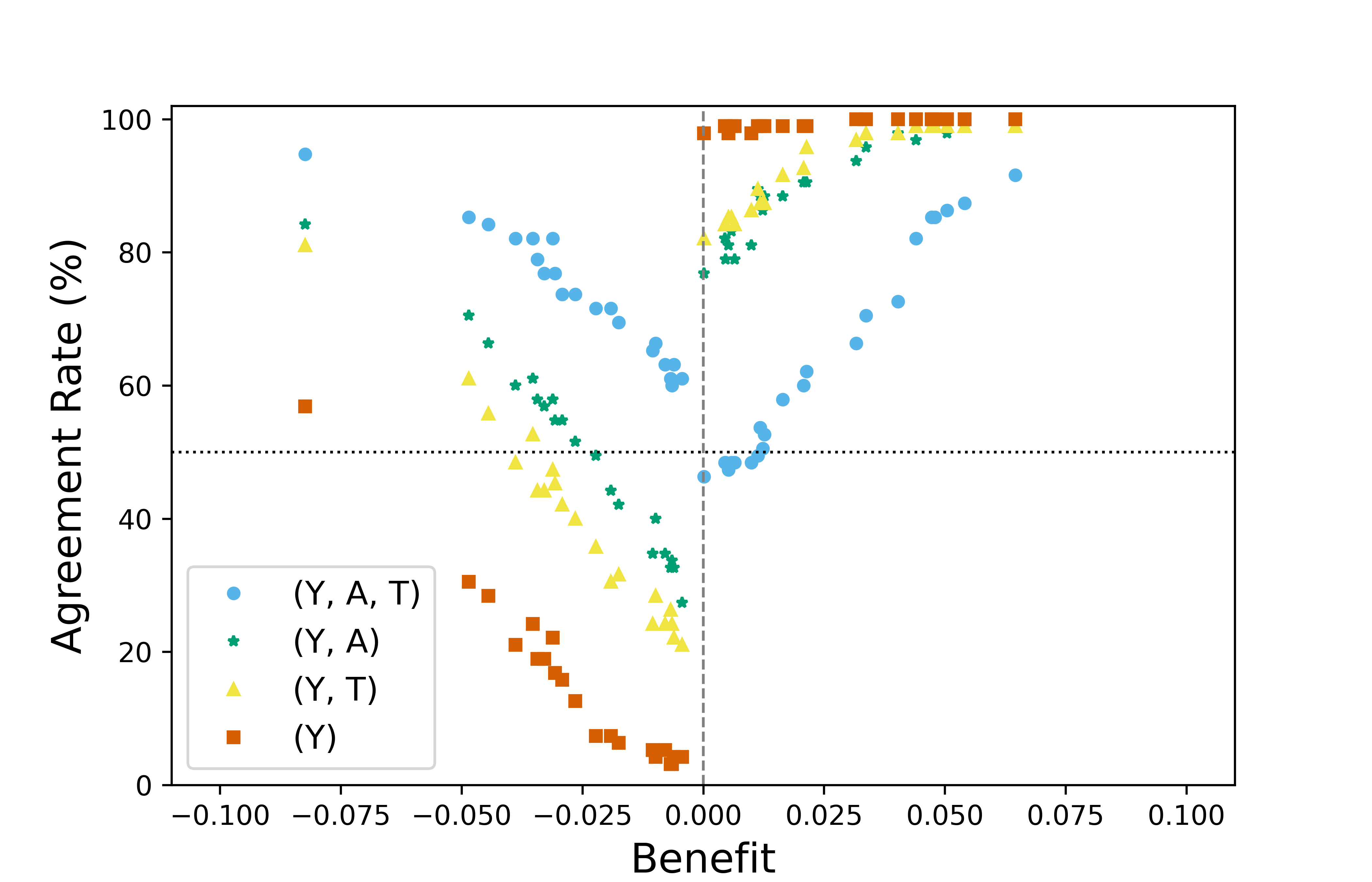
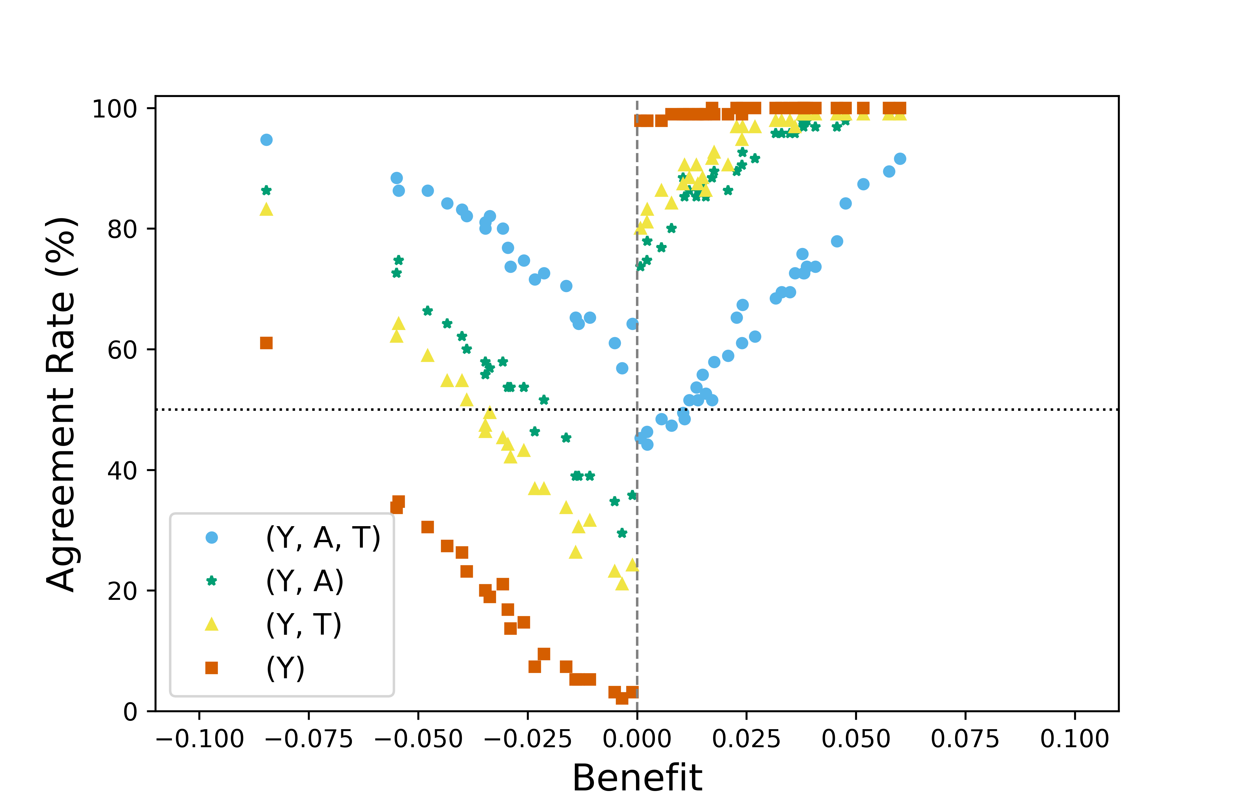
Figure 3: Benefit vs. agreement rate for all four model specifications given previous outcome $y_{i1}=0$ (left) and $y_{i1}=1$ (right).

In Figure 2, we observe the true benefit – reward difference under $(1,d_{3}^{\text{opt}})$ and $(0,d_{3}^{\text{opt}})$ – against the estimated loss, the difference in the estimated reward under estimated optimal regime $(\widehat{d}_{2}^{\text{opt}},\widehat{d}_{3}^{\text{opt}})$ and true optimal reward. We highlight that the bias estimates using $(Y,A,T)$ where all three processes are modeled are closest to 0 on average. For select individuals whose optimal regime is $(0,d_{3}^{\text{opt}})$, bias estimates from the $(Y,A,T)$ seem comparable to the ones from the $(Y,T)$ model and hover around the 0 mark, representing unbiasedness. The increase in the magnitude of estimated biases for the three partial models indicates in individuals whose optimal regime is $(1,d_{3}^{\text{opt}})$ that, in our simulation setting, treatment effectiveness seems over-estimated, with the $(Y)$ model performing the worse of all models. We provide bias and standard error estimates under optimal regime and fixed regimes in Appendix F.1 and F.2 respectively.

Similarly, in Figure 3, for individuals with a near-trivial benefit hovering around the 0 mark on the x-axis, we expect decision-makers to be ambivalent, i.e. having an AR around the 50% mark. As benefit increases, we expect ARs to increase and depart from the 50% mark and slowly converge to 100%. We observe this phenomenon for the full joint model $(Y,A,T)$, aligning with the finding from Figure 2 in that rewards estimates from $(Y,A,T)$ are best. We observe that the partial models are more polarized and biased, sometimes outright preferring one treatment regime over the other. Treatment effects seem to be overestimated in $(Y,A)$, $(Y,T)$ and $(Y)$ models. Given that $(1,d_{3}^{\text{opt}})$ is preferable over $(0,d_{3}^{\text{opt}})$ for around 57% of randomly generated individuals according to our simulation mechanism, this finding aligns well with the higher agreement rate of the partial models in individuals with positive benefit. Figures 2 and 3 highlight the importance of accurately estimating reward values under all treatment arms as the regime individualizing is a comparative process. We also report that, if random effects are generated under $(U_{i,\mathrm{W}},U_{i,\mathrm{A}})\perp\!\!\!\perp U_{i,\mathrm{T}}$ or $(U_{i,\mathrm{W}},U_{i,\mathrm{T}})\perp\!\!\!\perp U_{i,\mathrm{A}}$, estimation under partial models $(Y,A)$ and $(Y,T)$ is respectively equivalent to estimation under the full joint model $(Y,A,T)$; these results are also available in Appendix F.3. Lastly, we provide estimates of various standard errors and study the statistical significance of estimated bias in rewards in Appendix F.3.

4 Individualizing IL-7 Injection Cycles

4.1 INSPIRE 2 & 3 Trials

Human immunodeficiency virus (HIV) is a chronic disease primarily characterized by a depletion of CD4 cells leading to reduced immune system functionality (Douek et al., 2009). Highly active anti-retroviral therapy (HAART) replenishes CD4 cell count to a healthy threshold, i.e. above 500 cells/$\mu$L of blood, in HIV-infected individuals, enabling them to exhibit similar life expectancy as the non-infected (Douek et al., 2009). However, 15% to 30% of HIV-infected individuals fail to increase their CD4 count under HAART; such patients are referred to as low immunological responders (Levy et al., 2009). INSPIRE trials 2 and 3 were randomized trials which aimed to assess the benefits of repeated Interleukin-7 (IL-7) injections in low immunological responders as a means of increasing their CD4 cell count (Thiébaut et al., 2014, 2016). Data from the INSPIRE trials demonstrated that patients sustained an increase in CD4 cell count when given IL-7 injections (Thiébaut et al., 2014).

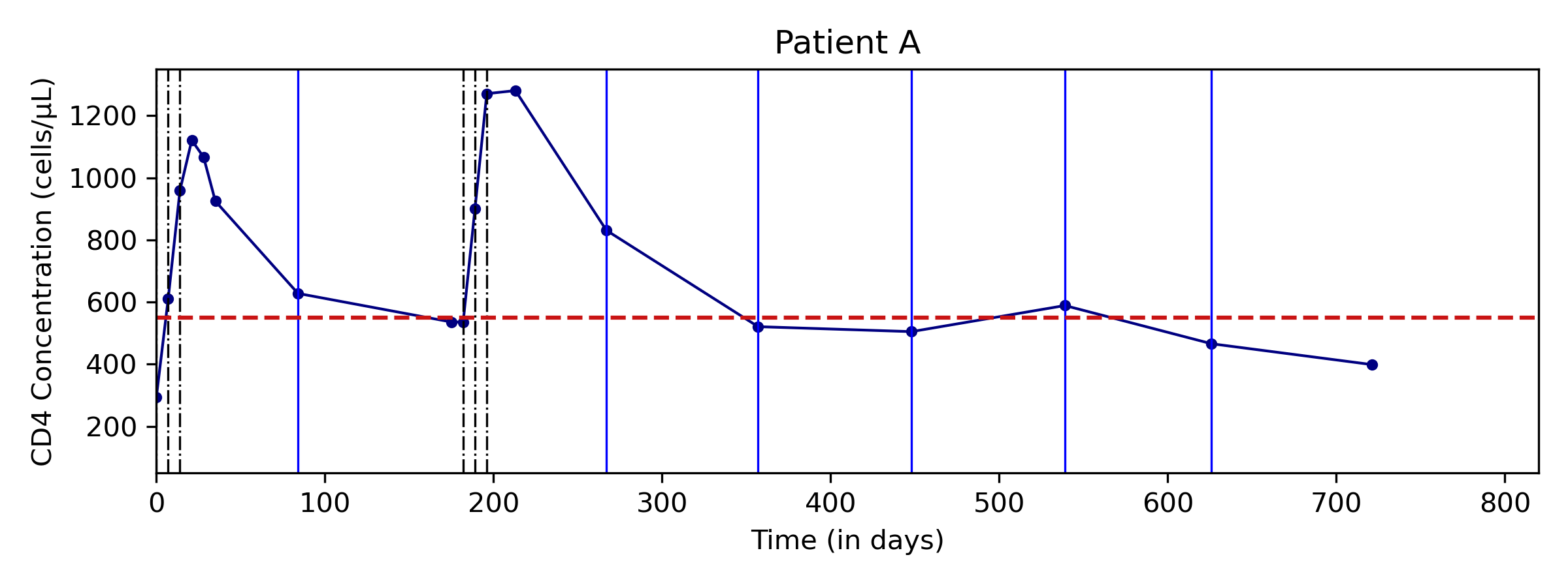
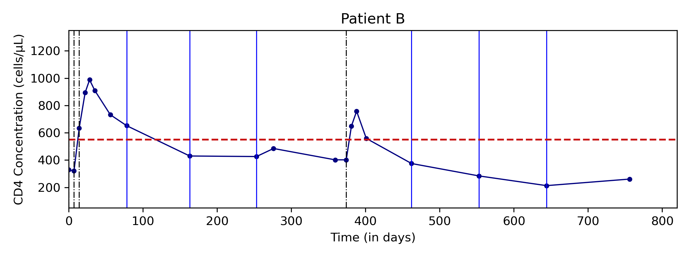
Figure 4: An example of the CD4 trajectory of two patients who has been observed for a total of around two years is displayed in Figure 4. Each dot represents a CD4 measurement. The vertical dashed-dot lines indicate administered injections and the solid vertical lines delineate approximate 90-windows around which investigators decided if injections were necessary or not.

The INSPIRE trials’ protocols calls for IL-7 injections at 20$\mu$g/Kg for each injection cycle administered at 90 day intervals if participants’ CD4 cell count falls below 550 cells/$\mu$L of blood (Thiébaut et al., 2016). However, this time interval varied between patients and within patient visits and participants also did not always receive all prescribed injections in a cycle when eligible.

4.2 Analysis Plan

4.2.1 Definition of Target Trial and Estimands

With $\operatorname{CD4}_{ij}$ being patient $i$’s CD4 measurement at visit $j\geqslant 1$, we define outcomes to be $Y_{ij}=\mathbbm{1}\left\{\operatorname{CD4}_{ij}\geqslant 500\right\}$ and $A_{ij}=1$ if an injection cycle was initiated at visit $j$, even if it was incomplete, and $0$ otherwise, akin to an intention-to-treat definition. We delineate the study designs of the INSPIRE trials and our target trial of interest as well as the observational setting in Appendix G.1. The applied problem is the following: given the 111 participant data from INSPIRE 2 and 3, we aim to optimize the injection cycles for the next year according to the target trial’s protocol, i.e. for the next four visits. We perform an in-depth analysis for two patients, whom we refer as “Patient A” and “Patient B”, whose trajectories are illustrative of two different patterns of sustained CD4 increase following IL-7 injections; their trajectories are displayed in Figure 4.

The nature of sustained levels of CD4 concentration, high or low, may not be well-explained by measured variables and could be captured through random effect modeling. Two baseline variables used for treatment tailoring are denoted by $X_{i0}$: BMI and age. We define a patient’s eligibility to receive injections at visit $j$ through a feasible set $\Psi_{j}(h_{j})=\{0,1\}$ if the total number of prior injections is two or less, otherwise $\Psi_{j}(h_{j})=\{0\}$.

Finally, employing the conditional reward defined in Section 2.2, we condition on one year’s worth of data for Patients A and B, i.e. $k=9$ for both individuals. Notably, patient A has received two injection cycles before day 365 whereas Patient B has only received one, since their second cycle starts at day 374. As such, given the feasible set definitions, Patient A would be eligible for a maximum of one more injections cycle whereas Patient B would eligible for up to two cycles. We are interested in optimizing treatment regimes for the next year, considering administering injections at 90-day intervals:

$$\mathcal{R}_{k}(h_{k},\underline{t}_{k},\underline{d}_{k}^{\text{opt}},\phi_{\mathcal{R}0})=\frac{1}{4}\sum_{j=k+1}^{k+4}\mathbb{E}_{\mathcal{E}}\big{[}Y_{j}\mid\overline{T}_{j}=\overline{t}_{j},\overline{A}_{j-1}=(\overline{a}_{k},d_{k}^{\text{opt}},\dots,d_{j-1}^{\text{opt}}),\overline{W}_{k}=\overline{w}_{k},\phi_{\mathcal{R}0}\big{]}\,.$$

Given that outcomes are binary, $\gamma_{j}=\frac{1}{4}$ for all $j$ allows the reward to be interpreted as an average probability across future outcomes. As a comparison, we also estimate rewards under a fixed regime “treat as early and as feasibly often as possible”, which we refer to as the “always treated” regime.

4.2.2 Bayesian Joint modeling of INSPIRE Data

The immediate rebounding of CD4 concentration after receiving IL-7 injections followed by a decaying effect with time can be seen in Figure 4; as such, we employ a dose-response (DR) relationship model to depict this phenomenon (Davidian and Giltinan, 2003). As above, we define a variable $Q_{ij}$ to be the indicator if patients have received any treatment before visit $j$ and $T_{ij}^{\text{last}}$ to be the time since the last injection if there were any and 0 otherwise.

$$Q_{ij}=\begin{cases}0&\quad\text{if }j=1\\ \mathbbm{1}\left[\sum_{k=1}^{j-1}A_{ik}>0\right]&\quad\text{if }j>1\end{cases}\,;\qquad T_{ij}^{\text{last}}=\begin{cases}0&\quad\text{if }Q_{ij}=0\\ T_{ij}-\max\big{\{}T_{ik}A_{ik}\big{\}}_{k=1}^{j-1}&\quad\text{if }Q_{ij}=1\end{cases}\,.$$

Moreover, we use an exponential function to mimic the rapid diminishing effects of IL-7 with increasing time without injections in defining $A_{ij}^{\text{DR}}=Q_{ij}\exp\left(-T_{ij}^{\text{last}}\eta_{i}\right)$ used in the outcome model, converging to 0 with increasing $T_{ij}^{\text{last}}$, and $\eta_{i}$ representing the individualized post-injection CD4 decay rate. Our model-specific regressors are: $H_{ij,\mathrm{A}}=\big{[}1,T_{ij}^{\text{last}},T_{ij}-T_{i(j-1)}\big{]}$, $H_{ij,\mathrm{Y}}=\big{[}1,A_{ij}^{\text{DR}},A_{ij}^{\text{DR}}*\operatorname{Age}_{i},A_{ij}^{\text{DR}}*\operatorname{BMI}_{i},Y_{i(j-1)}\big{]}$ and $H_{ij,\mathrm{T}}=\big{[}1,T_{ij}^{\text{last}},\operatorname{Phase}_{ij},\operatorname{Age}_{i},\operatorname{BMI}_{i}\big{]}$. In the following equations, we specify three model components: visit process, treatment assignment process and outcome process.

$$A_{ij}\mid\overline{T}_{ij},\overline{A}_{i(j-1)},\overline{Y}_{i(j-1)},X_{i0},\eta_{i},U_{i,\mathrm{A}},\phi_{\mathrm{A}} \sim\operatorname{Bern}\left(\Phi^{-1}\left(H_{ij,\mathrm{A}}^{\top}\phi_{\mathrm{A}}+U_{i,\mathrm{A}}\right)\right)$$

$$Y_{ij}\mid\overline{T}_{ij},\overline{A}_{i(j-1)},\overline{Y}_{i(j-1)},X_{i0},U_{i,\mathrm{Y}},\phi_{\mathrm{Y}} \sim\operatorname{Bern}\left(\Phi^{-1}\left(H_{ij,\mathrm{Y}}^{\top}\phi_{\mathrm{Y}}+U_{i,\mathrm{Y}}\right)\right)$$

$$T_{ij}-T_{i(j-1)}\mid\overline{A}_{i(j-1)},\overline{Y}_{i(j-1)},\overline{T}_{i(j-1)},\operatorname{Phase}_{ij},X_{i0},U_{i,\mathrm{T}},\phi_{T},\sigma_{\mathrm{T}}^{2} \sim\mathcal{N}\left(H_{ij,\mathrm{T}}^{\top}\phi_{T}+U_{i,\mathrm{T}},\sigma_{\mathrm{T}}^{2}\right)$$

The interarrival times $T_{ij}-T_{i(j-1)}$ were modeled using a Normal distribution, incorporating the protocol phase of the patient as a categorical variable. Given the ITT model for modeling the uptake of injection method, we employ a binomial GLM model with probit link. We exclude patient information from visits where they are receiving their second or third injection in a cycle, defining the first post-treatment observation as the initial “injection-free” visit following an IL-7 cycle. We consider correlated random intercepts $U_{i,\mathrm{T}},U_{i,\mathrm{W}},U_{i,\mathrm{A}}\mid\Sigma\sim\operatorname{MVN}\big{(}0,\Sigma\big{)}$ in the full joint model and similar conditional independence approaches in partial models $(Y,A)$, $(Y,T)$ and $(Y)$ as in the simulation study. We model the decay rate $\eta_{i}\mid\mu,\tau^{2}\sim\mathcal{N}(\mu,\tau^{2})$ and posit the following uninformative priors for our model parameters: $\phi_{\mathrm{T}}\sim\operatorname{MVN}\left(0,25\cdot\mathbf{I}_{\operatorname{dim}(\phi_{\mathrm{T}})}\right)$, $\sigma_{\mathrm{T}}^{2}\sim\operatorname{InvGamma}(0.1,0.1)$, $\phi_{\mathrm{A}}\sim\mathcal{N}(0,25\cdot\mathbf{I}_{\operatorname{dim}(\phi_{\mathrm{A}})})$, $\phi_{\mathrm{Y}}\sim\mathcal{N}(0,25\cdot\mathbf{I}_{\operatorname{dim}(\phi_{\mathrm{Y}})})$, $\mu\sim\mathcal{N}(0,25)$, $\tau^{2}\sim\operatorname{InvGamma}(0.1,0.1)$ and $\Sigma\sim\operatorname{InverseWishart}\big{(}\mathbf{I}_{3},3\big{)}$.

Four MCMC chains were run, each generating 100 000 samples, discarding the first 50 000 burn-in samples; traceplots for reward parameters $\phi_{\mathrm{Y}}$, $\phi_{\mathrm{U}}$, $\mu$ and $\tau^{2}$ are available in Appendix G.3. After applying a thinning interval of 10, G-computation was run on the 10 000 retained posterior samples to estimate the optimal and “always treated“ reward.

4.3 Data Analysis Results

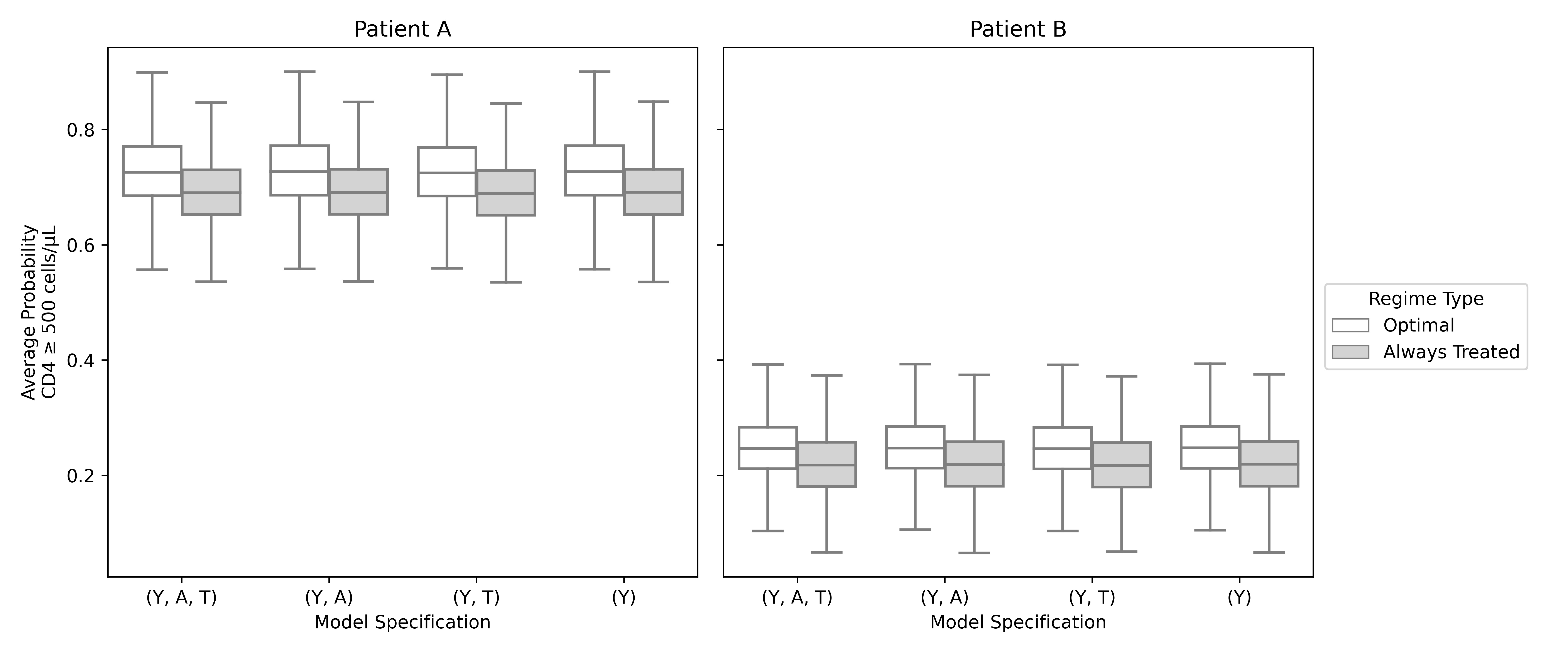
Figure 5: Estimated optimal reward under estimated optimal regime and estimated reward under an “always treated” regime for patients A and B under all four joint model specifications.

In Figure 5, we illustrate the posterior predictive rewards as boxplots if patient were seen for four more visits at 90 day intervals with treatment assigned under estimated optimal regime (in white) and under a fixed regime (in gray). From Figure 5, we can see that all four model specifications yield similar reward estimates under both regimes, indicating that little subject-specific heterogeneity underpinned the observational treatment and visit processes. As expected, the reward under an optimal rewards yields a larger value than under the “always treated” regime.

Under the full joint model $(Y,A,T)$ and estimated optimal regime, which we assume hereon, Patient A was recommended $\widehat{\underline{d}}_{k}^{\text{opt}}=(0,1,0,0)$ at a frequency of 64.9% followed by $(0,1,0,0)$ 29.0% of times whereas Patient B was recommended $(1,1,0,0)$ and $(1,0,1,0)$ respectively $54.5\%$ and $33.8\%$ of the time; more details of the frequency of treatment course recommendation is available in Appendix G.2. This result can be understood as the model recommending to treat as often as permitted, with the preferred timing to depend on patient’s history. For instance, from Figure 4, Patient A’s longitudinal CD4 measurements are on the higher side whereas Patient B’s CD4 count falls lower than Patient A. This explains why Patient A is more often recommended to receive an injection cycle after the first quarter than immediately whereas Patient B’s most recommended course of treatment to receive injections as soon as possible, if eligible. Moreover, given Patient’s A history, the average probability of having their CD4 count greater than 500 cells/$\mu$L is higher than Patient B’s. This reward estimation which is explainable through patient history stems from random effects $U_{i,\mathrm{Y}}$ and $\eta_{i}$ being sampled from a distribution conditional on observed history. Lastly, injection recommendation is not heavily affected by patient characteristics given the statistically insignificant estimates of tailoring variable coefficients based on 95% credible intervals; a summary of parameters from the fitted joint model is available in Table 8 in Appendix G.4. The similarity of results between model specifications can be attributed to the low correlation between model-specific random effects. While our proposed method and framework allows for correlated random effects, in this application the unobserved individual-level heterogeneity did not seem to be a major driver of the results.

5 Discussion and Conclusion

In this article, we first build upon the target trial paradigm using the decision theory framework from (Saarela et al., 2015) and (Yiu et al., 2022) to both articulate optimal multi-stage DTRs and incorporate visit time information. In the same spirit as the potential outcome framework, assumptions relating $\mathcal{E}$ and $\mathcal{O}$ settings handle well the continuous nature of visit times in the definition of the causal estimand, here optimal rewards and treatment regimes (Dawid and Didelez, 2010). Secondly, we propose using Bayesian joint modeling with irregular data to account for correlated random effects between different model components in estimating optimal treatment regimes and rewards. In particular, while Hua et al. (2022), Guan et al. (2020) and Oganisian et al. (2024) also explore Bayesian estimation of optimal DTRs with irregular data, our work studies the induced bias by ignoring the correlated structure of random effects and how this bias translates in the estimation procedure of optimal rewards.

Our notational framework assumes outcomes, covariates and treatments can only be measured at visits, akin to a marked point process. For instance, observational data collected from different data sources could have treatment assignments prescribed and clinical measurements taken on different days, requiring further refinement of our proposed framework. Moreover, our Bayesian joint model also makes strong parametric assumptions for the distribution of random effects, a restriction that can be relaxed in future work akin to Orihara et al. (2024). In the definition of our optimal rewards $\mathcal{R}_{k}(h_{k},\underline{t}_{k+1},\underline{d}_{k}^{\text{opt}},\phi_{\mathcal{R}0})$, we assume that future decision times $\underline{t}_{k+1}$ are chosen when defining the target trial of interest. Akin to Guan et al. (2020) and Hua et al. (2022), they could be part of the decision-making process and included in the definition of optimal DTRs. In principle, the proposed framework allows for optimization of visit times, but studying this is left as future work.

In the data analysis, we highlight several limitations. Akin to Villain et al. (2019) and Dong et al. (2023), the number of IL-7 injections can be included in the optimization procedure with a clearer articulation of the target trial. Secondly, in the spirit of retaining a parsimonious outcome model, only effect modifiers for the magnitude of injection benefits were looked into, in that we could also look into individualized effects of treatment decay. We also assume that the visit process random effect does not depend on the protocol phase, an assumption which can be relaxed since visit times in irregular data can vary more as a study progresses. Lastly, injection schedules and their visit times can themselves be optimized, motivating further methodological extension of this work.

To conclude, longitudinal observational data often feature irregular and informative observation times; we have shown that treating these times as non-informative can hinder identification of the optimal DTR and proposed a joint modeling approach to account for their informative nature. This, coupled with our target trial approach to identifying the causal estimand can be used to improve the rigor of DTR estimation.

Supplementary Materials to “Estimating Optimal Dynamic Treatment Regimes Using Irregularly Observed Data: A Target Trial Emulation and Bayesian Joint Modeling Approach”

Appendix A Characterizing Optimal Regimes via Optimal Decision Functions

A recursive definition of the reward $\mathcal{R}_{k}(h_{k},\underline{t}_{k+1},\underline{d}_{k}^{\text{opt}},\phi_{\mathcal{R}})$ can be used for any non-terminal stage $k$:

$$\quad\mathcal{R}_{k}(h_{k},\underline{t}_{k+1},\underline{d}_{k}^{\text{opt}},\phi_{\mathcal{R}})$$

$$=\gamma_{k+1}\mathbb{E}_{\mathcal{E}}\left[Y_{k+1}\mid\overline{T}_{k+1}=\overline{t}_{k+1},\overline{A}_{k}=\big{(}\overline{a}_{k-1},d_{k}^{\text{opt}}\big{)},\overline{W}_{k}=\overline{w}_{k},\phi_{\mathcal{R}}\right]$$

$$\quad+\sum_{j=k+2}^{K+1}\gamma_{j}\mathbb{E}_{\mathcal{E}}\left[Y_{j}\mid\overline{T}_{j}=\overline{t}_{j},\overline{A}_{j-1}=\big{(}\overline{a}_{k-1},d_{k}^{\text{opt}},\dots,d_{j-1}^{\text{opt}}\big{)},\overline{W}_{k}=\overline{w}_{k},\phi_{\mathcal{R}}\right]$$

$$=\gamma_{k+1}\mathbb{E}_{\mathcal{E}}\left[Y_{k+1}\mid\overline{T}_{k+1}=\overline{t}_{k+1},\overline{A}_{k}=\big{(}\overline{a}_{k-1},d_{k}^{\text{opt}}\big{)},\overline{W}_{k}=\overline{w}_{k},\phi_{\mathcal{R}}\right]$$

$$\qquad+\bigintsss_{w_{k+1}}\left\{\sum_{j=k+2}^{K+1}\gamma_{j}\mathbb{E}_{\mathcal{E}}\left[Y_{j}\mid\overline{T}_{j}=\overline{t}_{j},\overline{A}_{j-1}=\big{(}\overline{a}_{k-1},d_{k}^{\text{opt}},\dots,d_{j-1}^{\text{opt}}\big{)},\overline{W}_{k+1}=\overline{w}_{k+1},\phi_{\mathcal{R}}\right]\right\}$$

$$\hskip 56.9055pt\times f_{\mathcal{E}}\big{(}w_{k+1}\mid\overline{t}_{k+1},\big{(}\overline{a}_{k-1},d^{\text{opt}}_{k}(h_{k})\big{)},\overline{w}_{k},\phi_{\mathcal{R}0}\big{)}\,dw_{k+1}$$

$$=\gamma_{k+1}\mathbb{E}_{\mathcal{E}}\left[Y_{k+1}\mid\overline{T}_{k+1}=\overline{t}_{k+1},\overline{A}_{k}=\big{(}\overline{a}_{k-1},d_{k}^{\text{opt}}\big{)},\overline{W}_{k}=\overline{w}_{k},\phi_{\mathcal{R}}\right]$$

$$\qquad+\bigintsss_{w_{k+1}}\mathcal{R}_{k+1}(h_{k+1},\underline{t}_{k+2},\underline{d}^{\text{opt}}_{k+1},\phi_{\mathcal{R}})\,f_{\mathcal{E}}\big{(}w_{k+1}\mid\overline{t}_{k+1},\big{(}\overline{a}_{k-1},d^{\text{opt}}_{k}(h_{k})\big{)},\overline{w}_{k},\phi_{\mathcal{R}0}\big{)}\,dw_{k+1}\,.$$

As such, $d^{\text{opt}}_{j}$ for $j=k,\dots,K$ can be characterized recursively with $d_{K}^{\text{opt}}$ being the base case:

$$d_{K}^{\text{opt}}(h_{K},\phi_{\mathcal{R}}) =\operatorname*{argmax}_{d_{K}}\,\gamma_{K+1}\mathbb{E}_{\mathcal{E}}\left[Y_{k+1}\mid\overline{T}_{k+1}=\overline{t}_{K+1},\overline{A}_{K}=\big{(}\overline{a}_{K-1},d_{K}\big{)},\overline{W}_{K}=\overline{w}_{K},\phi_{\mathcal{R}}\right]$$

$$=\operatorname*{argmax}_{a_{K}\in\Psi_{K}(h_{K})}\,\gamma_{K+1}\mathbb{E}_{\mathcal{E}}\left[Y_{k+1}\mid\overline{T}_{k+1}=\overline{t}_{K+1},\overline{A}_{K}=\overline{a}_{K},\overline{W}_{K}=\overline{w}_{K},\phi_{\mathcal{R}}\right]$$

$$d_{j}^{\text{opt}}(h_{j},\phi_{\mathcal{R}}) =\operatorname*{argmax}_{d_{j}}\,\Bigg{\{}\gamma_{j+1}\mathbb{E}_{\mathcal{E}}\left[Y_{j+1}\mid\overline{T}_{j+1}=\overline{t}_{j+1},\overline{A}_{j}=\big{(}\overline{a}_{j-1},d_{j}\big{)},\overline{W}_{j}=\overline{w}_{j},\phi_{\mathcal{R}}\right]$$

$$\qquad+\bigintsss_{w_{j+1}}\mathcal{R}_{j+1}(h_{j+1},\underline{t}_{j+2},\underline{d}^{\text{opt}}_{j+1},\phi_{\mathcal{R}})\,f_{\mathcal{E}}\big{(}w_{j+1}\mid\overline{t}_{j+1},\big{(}\overline{a}_{j-1},d_{j}(h_{j})\big{)},\overline{w}_{j},\phi_{\mathcal{R}0}\big{)}\,dw_{j+1}\Bigg{\}}$$

$$=\operatorname*{argmax}_{a_{j}\in\Psi_{j}(h_{j})}\,\Bigg{\{}\gamma_{j+1}\mathbb{E}_{\mathcal{E}}\left[Y_{j+1}\mid\overline{T}_{j+1}=\overline{t}_{j+1},\overline{A}_{j}=\overline{a}_{j},\overline{W}_{j}=\overline{w}_{j},\phi_{\mathcal{R}}\right]$$

$$\qquad+\bigintsss_{w_{j+1}}\mathcal{R}_{j+1}(h_{j+1},\underline{t}_{j+2},\underline{d}^{\text{opt}}_{j+1},\phi_{\mathcal{R}})\,f_{\mathcal{E}}(w_{j+1}\mid\overline{t}_{j+1},\overline{a}_{j},\overline{w}_{j},\phi_{\mathcal{R}0})\,dw_{j+1}\Bigg{\}}\,.$$

Appendix B Derivation of Rewards

First, we begin with factorizing $f_{\mathcal{E}}(\overline{w}_{j+1},\overline{t}_{j+1},\overline{a}_{j}\mid u,\phi_{\mathrm{W}},\phi_{\mathrm{T}}^{*},\phi_{\mathrm{A}}^{*})$ for any $j=1,\dots,J$:

$$\quad f_{\mathcal{E}}(\overline{w}_{j+1},\overline{t}_{j+1},\overline{a}_{j}\mid u,\phi_{\mathrm{W}},\phi_{\mathrm{T}}^{*},\phi_{\mathrm{A}}^{*})$$

$$=f_{\mathcal{E}}(w_{j+1},t_{j+1}\mid\overline{w}_{j},\overline{t}_{j},\overline{a}_{j},u_{\mathrm{W}},u_{\mathrm{T}},\phi_{\mathrm{W}},\phi_{\mathrm{T}}^{*})\left\{\prod_{\ell=1}^{j}f_{\mathcal{E}}(a_{\ell},w_{\ell},t_{\ell}\mid\overline{a}_{\ell-1},\overline{w}_{\ell-1},\overline{t}_{\ell-1},u,\phi_{\mathrm{W}},\phi_{\mathrm{T}}^{*},\phi_{\mathrm{A}}^{*})\right\}$$

$$=f_{\mathcal{E}}(w_{j+1}\mid\overline{t}_{j+1},\overline{w}_{j},\overline{a}_{j},u_{\mathrm{W}},\phi_{\mathrm{W}})\,f_{\mathcal{E}}(t_{j+1}\mid\overline{w}_{j},\overline{t}_{j},\overline{a}_{j},u_{\mathrm{T}},\phi_{\mathrm{T}}^{*})$$

$$\quad\times\left\{\prod_{\ell=1}^{j}f_{\mathcal{E}}(a_{\ell}\mid\overline{w}_{\ell},\overline{t}_{\ell},\overline{a}_{\ell-1},u_{\mathrm{A}},\phi_{\mathrm{A}}^{*})f_{\mathcal{E}}(w_{\ell}\mid\overline{t}_{\ell},\overline{a}_{\ell-1},\overline{w}_{\ell-1},u_{\mathrm{W}},\phi_{\mathrm{W}})f_{\mathcal{E}}(t_{\ell}\mid\overline{a}_{\ell-1},\overline{w}_{\ell-1},\overline{t}_{\ell-1},u_{\mathrm{T}},\phi_{\mathrm{T}}^{*})\right\}$$

$$=\left\{\prod_{\ell=1}^{j+1}f_{\mathcal{E}}(w_{\ell}\mid\overline{t}_{\ell},\overline{a}_{\ell-1},\overline{w}_{\ell-1},u_{\mathrm{W}},\phi_{\mathrm{W}})\right\}\left\{\prod_{\ell=1}^{j+1}f_{\mathcal{E}}(t_{\ell}\mid\overline{a}_{\ell-1},\overline{w}_{\ell-1},\overline{t}_{\ell-1},u_{\mathrm{T}},\phi_{\mathrm{T}}^{*})\right\}$$

$$\quad\times\left\{\prod_{\ell=1}^{j}f_{\mathcal{E}}(a_{\ell}\mid\overline{w}_{\ell},\overline{t}_{\ell},\overline{a}_{\ell-1},u_{\mathrm{A}},\phi_{\mathrm{A}}^{*})\right\}$$

$$=\left\{\prod_{\ell=1}^{j+1}f_{\mathcal{E}}(w_{\ell}\mid\overline{t}_{\ell},\overline{a}_{\ell-1},\overline{w}_{\ell-1},u_{\mathrm{W}},\phi_{\mathrm{W}})\right\}\left\{\prod_{\ell=1}^{j+1}f_{\mathcal{E}}(t_{\ell}\mid\overline{a}_{\ell-1},\overline{t}_{\ell-1},u_{\mathrm{T}},\phi_{\mathrm{T}}^{*})\right\}$$

$$\quad\times\left\{\prod_{\ell=1}^{j}f_{\mathcal{E}}(a_{\ell}\mid\overline{t}_{\ell-1},\overline{a}_{\ell-1},u_{\mathrm{A}},\phi_{\mathrm{A}}^{*})\right\}$$

$$=\left\{\prod_{\ell=1}^{j+1}f_{\mathcal{E}}(w_{\ell}\mid\overline{t}_{\ell},\overline{a}_{\ell-1},\overline{w}_{\ell-1},u_{\mathrm{W}},\phi_{\mathrm{W}})\right\}f_{\mathcal{E}}(\overline{t}_{j+1},\overline{a}_{j}\mid u_{\mathrm{A}},u_{\mathrm{T}},\phi_{\mathrm{A}}^{*},\phi_{\mathrm{T}}^{*})$$

$$=\left\{\prod_{\ell=1}^{j+1}f_{\mathcal{E}}(w_{\ell}\mid\overline{t}_{\ell},\overline{a}_{\ell-1},\overline{w}_{\ell-1},u_{\mathrm{W}},\phi_{\mathrm{W}})\right\}f_{\mathcal{E}}(\overline{t}_{j+1},\overline{a}_{j}\mid\phi_{\mathrm{A}}^{*},\phi_{\mathrm{T}}^{*})\,.$$

The third to last equation is obtained from using the specifications of treatment and observation processes under $\mathcal{E}$ as per A3. Using the derivation above, we can show that $f_{\mathcal{E}}(\overline{w}_{j}\mid\overline{t}_{j},\overline{a}_{j-1},u_{\mathrm{W}},\phi_{\mathrm{W}})$ factorizes into a product of conditional distributions:

$$\qquad f_{\mathcal{E}}(\overline{w}_{j}\mid\overline{t}_{j},\overline{a}_{j-1},u_{\mathrm{W}},\phi_{\mathrm{W}},\phi_{\mathrm{A}}^{*},\phi_{\mathrm{T}}^{*})$$

$$=\frac{f_{\mathcal{E}}(\overline{w}_{j},\overline{t}_{j},\overline{a}_{j-1}\mid u,\phi_{\mathrm{W}},\phi_{\mathrm{A}}^{*},\phi_{\mathrm{T}}^{*})}{f_{\mathcal{E}}(\overline{t}_{j},\overline{a}_{j-1}\mid u,\phi_{\mathrm{A}}^{*},\phi_{\mathrm{T}}^{*})}$$

$$=\frac{\left\{\prod_{\ell=1}^{j}f_{\mathcal{E}}(w_{\ell}\mid\overline{t}_{\ell},\overline{a}_{\ell-1},\overline{w}_{\ell-1},u_{\mathrm{W}},\phi_{\mathrm{W}})\right\}f_{\mathcal{E}}(\overline{t}_{j},\overline{a}_{j-1}\mid\phi_{\mathrm{A}}^{*},\phi_{\mathrm{T}}^{*})}{f_{\mathcal{E}}(\overline{t}_{j},\overline{a}_{j-1}\mid\phi_{\mathrm{A}}^{*},\phi_{\mathrm{T}}^{*})}$$ using the previous derivation

$$=\frac{\left\{\prod_{\ell=1}^{j}f_{\mathcal{E}}(w_{\ell}\mid\overline{t}_{\ell-1},\overline{a}_{\ell-1},\overline{w}_{\ell-1},u_{\mathrm{W}},\phi_{\mathrm{W}})\right\}\cancel{f_{\mathcal{E}}(\overline{t}_{j},\overline{a}_{j-1}\mid\phi_{\mathrm{A}}^{*},\phi_{\mathrm{T}}^{*})}}{\cancel{f_{\mathcal{E}}(\overline{t}_{j},\overline{a}_{j-1}\mid\phi_{\mathrm{A}}^{*},\phi_{\mathrm{T}}^{*})}}$$

$$=\prod_{\ell=1}^{j}f_{\mathcal{E}}(w_{\ell}\mid\overline{t}_{\ell-1},\overline{a}_{\ell-1},\overline{w}_{\ell-1},u_{\mathrm{W}},\phi_{\mathrm{W}})$$

The density from the conditional reward $f_{\mathcal{E}}(w_{j}\mid\overline{t}_{j},\overline{a}_{j-1},\overline{w}_{k},u_{\mathrm{W}},\phi_{\mathrm{W}})$ only conditions on partial observations $\overline{W}_{k}=\overline{w}_{k}$. For $j>k+1$, we express it as:

$$\qquad f_{\mathcal{E}}(w_{j}\mid\overline{t}_{j},\overline{a}_{j-1},\overline{w}_{k},u_{\mathrm{W}},\phi_{\mathrm{W}})$$

$$=\bigintsss_{w_{k+1}}\dots\bigintsss_{w_{j+1}}f_{\mathcal{E}}(w_{k+1},\dots,w_{j+1},w_{j}\mid\overline{t}_{j},\overline{a}_{j-1},\overline{w}_{j-1},u_{\mathrm{W}},\phi_{\mathrm{W}})\,dw_{j+1}\dots\,dw_{k+1}\,du_{\mathrm{W}}\,.$$

The stage $j>k$ expected outcome conditional can then be rewritten:

$$\qquad\mathbb{E}_{\mathcal{E}}\left[Y_{j}\mid\overline{T}_{j}=\overline{t}_{j},\overline{A}_{j-1}=\overline{d}_{j-1},\overline{W}_{k}=\overline{w}_{k},\phi_{\mathcal{R}}\right]$$

$$=\bigintsss_{u_{\mathrm{W}}}\bigintsss_{w_{j}}y_{j}\,f_{\mathcal{E}}(w_{j}\mid\overline{t}_{j},\overline{a}_{j-1},\overline{w}_{k},u_{\mathrm{W}},\phi_{\mathrm{W}})\,f_{\mathcal{E}}(u_{\mathrm{W}}\mid\overline{t}_{j},\overline{a}_{j-1},\overline{w}_{j-1}\phi_{\mathrm{U}})\,\,dw_{j}\,du_{\mathrm{W}}$$

$$=\bigintsss_{u_{\mathrm{W}}}\bigintsss_{w_{k+1}}\dots\bigintsss_{w_{j}}y_{k}\,\prod_{\ell=k+1}^{j}f_{\mathcal{E}}(w_{\ell}\mid\overline{t}_{\ell-1},\overline{a}_{\ell-1},\overline{w}_{\ell-1},u_{\mathrm{W}},\phi_{\mathrm{W}})\,f_{\mathcal{E}}(u_{\mathrm{W}}\mid\overline{t}_{j},\overline{a}_{j-1},\overline{w}_{j-1}\phi_{\mathrm{U}})\,dw_{j}\dots\,dw_{k+1}\,du_{\mathrm{W}}\,.$$

Using this, we can then rewrite our reward $\mathcal{R}_{k}(h_{k},\underline{t}_{k+1},\underline{d}_{k},\phi_{\mathcal{R}})$ using conditional distributions of the two following forms: $f_{\mathcal{E}}(w_{j}\mid\overline{t}_{j},\overline{a}_{j-1},\overline{w}_{j-1},u_{\mathrm{W}},\phi_{\mathrm{W}})$ for some $j\leqslant K+1$ and $f_{\mathcal{E}}(u_{\mathrm{W}}\mid\phi_{\mathrm{U}})$. Grouping several alike terms and using Bayes’ formula from the third to fourth step yields the following derivation:

$$\qquad\mathcal{R}_{k}(h_{k},\underline{t}_{k+1},\underline{d}_{k},\phi_{\mathcal{R}})$$

$$=\sum_{j=k+1}^{K+1}\gamma_{j}\mathbb{E}_{\mathcal{E}}\left[Y_{j}\mid\overline{T}_{j}=\overline{t}_{j},\overline{A}_{j-1}=\overline{d}_{j-1},\overline{W}_{k}=\overline{w}_{k},\phi_{\mathcal{R}}\right]$$

$$=\bigintsss_{u_{\mathrm{W}}}\left\{\sum_{j=k+1}^{K+1}\gamma_{j}\mathbb{E}_{\mathcal{E}}\left[Y_{j}\mid\overline{T}_{j}=\overline{t}_{j},\overline{A}_{j-1}=\overline{d}_{j-1},\overline{W}_{k}=\overline{w}_{k},u_{\mathrm{W}},\phi_{\mathrm{W}}\right]\right\}f_{\mathcal{E}}(u_{\mathrm{W}}\mid\overline{t}_{k},\overline{w}_{k},\overline{d}_{k-1},\phi_{\mathcal{R}})\,du_{\mathrm{W}}$$

$$=\bigintsss_{u_{\mathrm{W}}}\Bigg{\{}\bigintsss_{w_{k+1}}\dots\bigintsss_{w_{K+1}}\sum_{j=k+1}^{K+1}\gamma_{j}y_{j}\prod_{j=k+1}^{K+1}f_{\mathcal{E}}(w_{j}\mid\overline{t}_{j},\overline{d}_{j-1},\overline{w}_{j-1},u_{\mathrm{W}},\phi_{\mathrm{W}})\,\,dw_{K+1}\dots\,dw_{j+1}\Bigg{\}}$$

$$\qquad\times f_{\mathcal{E}}(u_{\mathrm{W}}\mid\overline{w}_{j},\overline{t}_{j},\overline{d}_{j-1},\phi_{\mathcal{R}})\,du_{\mathrm{W}}$$

$$=\bigintsss_{u_{\mathrm{W}}}\Bigg{\{}\bigintsss_{w_{k+1}}\dots\bigintsss_{w_{K+1}}\sum_{j=k+1}^{K+1}\gamma_{j}y_{j}\prod_{j=k+1}^{K+1}f_{\mathcal{E}}(w_{j}\mid\overline{t}_{j},\overline{d}_{j-1},\overline{w}_{j-1},u_{\mathrm{W}},\phi_{\mathrm{W}})\,\,dw_{K+1}\dots\,dw_{k+1}\Bigg{\}}$$

$$\qquad\times\frac{\left\{\prod_{j=1}^{k}f_{\mathcal{E}}(w_{j}\mid\overline{t}_{j},\overline{d}_{j-1},\overline{w}_{j-1},u_{\mathrm{W}},\phi_{\mathrm{W}})\right\}f_{\mathcal{E}}(u_{\mathrm{W}}\mid\phi_{\mathrm{U}})}{\bigintss_{u_{\mathrm{W}}}\left\{\prod_{j=1}^{k}f_{\mathcal{E}}(w_{k}\mid\overline{t}_{k},\overline{d}_{k-1},\overline{w}_{k-1},u_{\mathrm{W}},\phi_{\mathrm{W}})\right\}f_{\mathcal{E}}(u_{\mathrm{W}}\mid\phi_{\mathrm{U}})\,du_{\mathrm{W}}}\,du_{\mathrm{W}}$$

$$=\bigintsss_{u_{\mathrm{W}}}\bigintsss_{w_{k+1}}\dots\bigintsss_{w_{K+1}}\left\{\sum_{j=k+1}^{K+1}\gamma_{j}y_{j}\right\}$$

$$\qquad\times\frac{\left\{\prod_{j=1}^{K+1}f_{\mathcal{E}}(w_{j}\mid\overline{t}_{j},\overline{d}_{j-1},\overline{w}_{j-1},u_{\mathrm{W}},\phi_{\mathrm{W}})\right\}f_{\mathcal{E}}(u_{\mathrm{W}}\mid\phi_{\mathrm{U}})}{\bigintss_{u_{\mathrm{W}}}\left\{\prod_{j=1}^{k}f_{\mathcal{E}}(w_{j}\mid\overline{t}_{j},\overline{d}_{j-1},\overline{w}_{j-1},u_{\mathrm{W}},\phi_{\mathrm{W}})\right\}f_{\mathcal{E}}(u_{\mathrm{W}}\mid\phi_{\mathrm{U}})\,du_{\mathrm{W}}}\,dw_{K+1}\dots\,dw_{k+1}\,du_{\mathrm{W}}\,,$$

where the last step in the derivation above combines products of $f_{\mathcal{E}}(w_{j}\mid\overline{t}_{j},\overline{d}_{j-1},\overline{w}_{j-1},u_{\mathrm{W}},\phi_{\mathrm{W}})$ for indices $j=1,\dots,k$ and $j=k+1,\dots,K+1$.

Appendix C Extended G-Computation Proof

Proof.

We make use of assumptions A1, A2 and A4 to convert $\mathcal{E}-$distributions into $\mathcal{O}-$distributions. We start with the ratio of $\mathcal{E}$ and $\mathcal{O}$ random effects $u_{\mathrm{W}}$ to be equal to 1:

$$\frac{f_{\mathcal{O}}(u_{\mathrm{W}}\mid\phi_{\mathrm{U}})}{f_{\mathcal{E}}(u_{\mathrm{W}}\mid\phi_{\mathrm{U}})}=1\,,$$

for all possible $u_{\mathrm{W}}$ due to A3. We also consider the following importance sampling ratio:

$$\frac{f_{\mathcal{O}}(w_{k}\mid\overline{t}_{k},\overline{d}_{k-1},\overline{w}_{k-1},u_{\mathrm{W}},\phi_{\mathrm{W}})}{f_{\mathcal{E}}(w_{k}\mid\overline{t}_{k},\overline{d}_{k-1},\overline{w}_{k-1},u_{\mathrm{W}},\phi_{\mathrm{W}})}=1$$

to be well-defined, i.e. have a non-zero denominator, due to A4 and to be equal to $1$ for any $k=1,\dots,K+1$ due to A2. With these stability assumptions, we directly convert $\mathcal{E}$ to $\mathcal{O}$ densities through direct substitions

$$\qquad\mathcal{R}_{k}(h_{k},\underline{t}_{k+1},\underline{d}_{k},\phi_{\mathcal{R}})$$

$$=\bigintsss_{u_{\mathrm{W}}}\bigintsss_{w_{k+1}}\dots\bigintsss_{w_{K+1}}\sum_{j=k+1}^{K+1}\gamma_{j}y_{j}$$

$$\quad\times\frac{\left\{\prod_{j=k+1}^{K+1}f_{\mathcal{E}}(w_{j}\mid\overline{t}_{j},\overline{d}_{j-1},\overline{w}_{j-1},u_{\mathrm{W}},\phi_{\mathrm{W}})\right\}f_{\mathcal{E}}(u_{\mathrm{W}}\mid\phi_{\mathrm{U}})}{\bigintss_{u_{\mathrm{W}}}\left\{\prod_{j=1}^{k}f_{\mathcal{E}}(w_{j}\mid\overline{t}_{j},\overline{d}_{j-1},\overline{w}_{j-1},u_{\mathrm{W}},\phi_{\mathrm{W}})\right\}f_{\mathcal{E}}(u_{\mathrm{W}}\mid\phi_{\mathrm{U}})du_{\mathrm{W}}}\,dw_{K+1}\dots dw_{k+1}du_{\mathrm{W}}$$

$$=\bigintsss_{u_{\mathrm{W}}}\bigintsss_{w_{k+1}}\dots\bigintsss_{w_{K+1}}\sum_{j=k+1}^{K+1}\gamma_{j}y_{j}$$

$$\quad\times\frac{\left\{\prod_{j=k+1}^{K+1}f_{\mathcal{O}}(w_{j}\mid\overline{t}_{j},\overline{d}_{j-1},\overline{w}_{j-1},u_{\mathrm{W}},\phi_{\mathrm{W}})\right\}f_{\mathcal{O}}(u_{\mathrm{W}}\mid\phi_{\mathrm{U}})}{\bigintss_{u_{\mathrm{W}}}\left\{\prod_{j=1}^{k}f_{\mathcal{O}}(w_{j}\mid\overline{t}_{j},\overline{d}_{j-1},\overline{w}_{j-1},u_{\mathrm{W}},\phi_{\mathrm{W}})\right\}f_{\mathcal{O}}(u_{\mathrm{W}}\mid\phi_{\mathrm{U}})du_{\mathrm{W}}}\,dw_{K+1}\dots dw_{k+1}du_{\mathrm{W}}\,.$$

The positivity assumption A4 is implicitly used when evoking $f_{\mathcal{E}}(w_{j}\mid\overline{t}_{j},\overline{a}_{j-1},\overline{w}_{j-1},u_{\mathrm{W}},\phi_{\mathrm{W}})$ where the conditional set must have non-zero density. Given that rewards are defined under $\mathcal{E}$, we require that the measure of the conditional set $(\overline{t}_{j},\overline{a}_{j-1},\overline{w}_{j-1})$ under $\mathcal{E}$ be absolutely continuous respect to its $\mathcal{O}$ analogue, i.e.:

$$f_{\mathcal{E}}(\overline{t}_{j},\overline{a}_{j-1},\overline{w}_{j-1})>0 \Rightarrow f_{\mathcal{O}}(\overline{t}_{k},\overline{a}_{j-1},\overline{w}_{j-1})>0$$

$$\Leftrightarrow f_{\mathcal{E}}(\overline{t}_{j},\overline{a}_{j-1},\overline{w}_{j-1}\mid u,\phi_{\mathrm{W}},\phi_{\mathrm{A}}^{*},\phi_{\mathrm{T}}^{*})>0 \Rightarrow f_{\mathcal{O}}(\overline{t}_{j},\overline{a}_{j-1},\overline{w}_{j-1}\mid u,\phi)>0\qquad(*)$$

for all $j=1,\dots,K+1$ and all possible $u,\phi,\phi_{\mathrm{A}}^{*},\phi_{\mathrm{T}}^{*}$ values. Akin to the factorization in B, the densities can be expressed as:

$$f_{\mathcal{E}}(\overline{t}_{j},\overline{a}_{j-1},\overline{w}_{j-1}\mid u,\phi_{\mathrm{W}},\phi_{\mathrm{A}}^{*},\phi_{\mathrm{T}}^{*}) =\left\{\prod_{\ell=1}^{j}f_{\mathcal{E}}(t_{\ell}\mid\overline{a}_{\ell-1},\overline{t}_{\ell-1},u_{\mathrm{T}},\phi_{\mathrm{T}}^{*})\right\}\left\{\prod_{\ell=1}^{j-1}f_{\mathcal{E}}(a_{\ell}\mid\overline{t}_{\ell-1},\overline{a}_{\ell-1},u_{\mathrm{A}},\phi_{\mathrm{A}}^{*})\right\}$$

$$\quad\times\ \left\{\prod_{\ell=1}^{j-1}f_{\mathcal{E}}(w_{\ell}\mid\overline{t}_{\ell},\overline{a}_{\ell-1},\overline{w}_{\ell-1},u_{\mathrm{W}},\phi_{\mathrm{W}})\right\}$$

$$f_{\mathcal{O}}(\overline{t}_{j},\overline{a}_{j-1},\overline{w}_{j-1}\mid u,\phi) =\left\{\prod_{\ell=1}^{j}f_{\mathcal{O}}(t_{\ell}\mid\overline{a}_{\ell-1},\overline{w}_{\ell-1},\overline{t}_{\ell-1},u_{\mathrm{T}},\phi_{\mathrm{T}})\right\}$$

$$\quad\times\left\{\prod_{\ell=1}^{j-1}f_{\mathcal{O}}(w_{\ell}\mid\overline{t}_{\ell},\overline{a}_{\ell-1},\overline{w}_{\ell-1},u_{\mathrm{W}},\phi_{\mathrm{W}})\right\}$$

$$\quad\times\left\{\prod_{\ell=1}^{j-1}f_{\mathcal{O}}(a_{\ell}\mid\overline{t}_{\ell-1},\overline{a}_{\ell-1},\overline{w}_{\ell-1},u_{\mathrm{A}},\phi_{\mathrm{A}})\right\}\,.$$

The factorization of joint densities can be incorporated into the condition $(*)$ above. Under A2, it simplifies to $f_{\mathcal{E}}(t_{j+1}\mid\overline{a}_{j},\overline{t}_{j},\phi_{\mathrm{T}}^{*})>0\Rightarrow f_{\mathcal{O}}(t_{j+1}\mid\overline{a}_{j},\overline{t}_{j},\overline{w}_{j},u_{\mathrm{T}},\phi_{\mathrm{T}})>0$ and $f_{\mathcal{E}}(a_{j}\mid\overline{t}_{j},\overline{a}_{j-1},\phi_{\mathrm{A}}^{*})>0\Rightarrow f_{\mathcal{O}}(a_{j}\mid\overline{w}_{j},\overline{t}_{j},\overline{a}_{j},u_{\mathrm{A}},\phi_{\mathrm{A}})>0$ for any $j$, which is the positivity assumption posited in A4. ∎

Appendix D Posterior Estimation of Rewards

D.1 Justification of Bayesian Estimator via de Finetti’s Representation Theorem

Following Saarela et al. (2023), we show that the rewards for a yet-to-be-observed individual $i>n$ evaluated at the true $\phi_{\mathrm{W}0}$ value is the limiting case of an expression that would serve as a natural Bayesian estimator using de Finetti’s Representation Theorem.

$$\quad\lim_{n\rightarrow\infty}\mathbb{E}_{\mathcal{E}}\left[Y_{j}\mid\overline{T}_{j}=\overline{t}_{j},\overline{A}_{j-1}=\overline{d}_{j-1},\overline{W}_{j-1}=\overline{w}_{j-1},\mathcal{F}_{n}\right]$$

$$=\lim_{n\rightarrow\infty}\bigintsss_{\phi_{\mathcal{R}}}\bigintsss_{u_{\mathrm{W}}}\mathbb{E}_{\mathcal{E}}\left[Y_{j}\mid\overline{T}_{j}=\overline{t}_{j},\overline{A}_{j-1}=\overline{d}_{j-1},\overline{W}_{j-1}=\overline{w}_{j-1},u_{\mathrm{W}},\phi_{\mathrm{W}}\right]f_{\mathcal{O}}(u_{\mathrm{W}}\mid\phi_{\mathrm{U}})\,\pi_{n}(d\phi_{\mathcal{R}})$$

$$=\bigintsss_{\phi_{\mathcal{R}}}\bigintsss_{u_{\mathrm{W}}}\mathbb{E}_{\mathcal{E}}\left[Y_{j}\mid\overline{T}_{j}=\overline{t}_{j},\overline{A}_{j-1}=\overline{d}_{j-1},\overline{W}_{j-1}=\overline{w}_{j-1},u_{\mathrm{W}}\right]f_{\mathcal{O}}(u_{\mathrm{W}}\mid\phi_{\mathrm{U}})\,\delta_{\phi_{\mathcal{R}0}}(d\phi_{\mathcal{R}})$$

$$=\mathbb{E}_{\mathcal{E}}\left[Y_{j}\mid\overline{T}_{j}=\overline{t}_{j},\overline{A}_{j-1}=\overline{d}_{j-1},\overline{W}_{j-1}=\overline{w}_{j-1},\phi_{\mathcal{R}0}\right]\,,$$

which is the $j$th stage intermediate reward under visit times $\overline{t}_{j}$, treatments $\overline{a}_{j-1}$ and the true parameter values $\phi_{\mathcal{R}0}$, assuming that the posterior converges to a degenerate distribution at $\phi_{\mathcal{R}0}$. The last equality uses $Y_{j}\perp\!\!\!\perp\mathcal{F}_{n}\mid\phi$ for $1\leqslant j\leqslant K$, $i\notin\{1,\dots,n\}$ from the representation theorem. With finite $n$, the above can be approximated by the posterior predictive expectation:

$$\qquad\mathbb{E}_{\mathcal{E}}\left[Y_{j}\mid\overline{T}_{j}=\overline{t}_{j},\overline{A}_{j-1}=\overline{d}_{j-1},\overline{W}_{j-1}=\overline{w}_{j-1},\phi_{\mathcal{R}0}\right]$$

$$\approx\mathbb{E}_{\mathcal{E}}\left[Y_{j}\mid\overline{T}_{j}=\overline{t}_{j},\overline{A}_{j-1}=\overline{a}_{j-1},\overline{W}_{j-1}=\overline{w}_{j-1},\mathcal{F}_{n}\right]$$

$$=\bigintsss_{\phi_{\mathcal{R}}}\mathbb{E}_{\mathcal{E}}\left[Y_{j}\mid\overline{T}_{j}=\overline{t}_{j},\overline{A}_{j-1}=\overline{a}_{j-1},\overline{W}_{j-1}=\overline{w}_{j-1},\phi_{\mathcal{R}}\right]\,\pi_{n}(d\phi_{\mathcal{R}})$$

$$\approx\frac{1}{B}\sum_{b=1}^{B}\mathbb{E}_{\mathcal{E}}\left[Y_{j}\mid\overline{T}_{j}=\overline{t}_{j},\overline{A}_{j-1}=\overline{a}_{j-1},\overline{W}_{j-1}=\overline{w}_{j-1},\phi_{\mathcal{R}}^{(b)}\right]\,,$$

where $\big{\{}\phi_{\mathcal{R}}^{(b)}\big{\}}_{b=1}^{B}$ are drawn from $\pi_{n}(\phi_{\mathcal{R}})$ following an MCMC procedure.

D.2 Monte Carlo Approximation to Optimal and Non-Optimal Rewards

We also introduce a Monte Carlo estimation procedure to estimate reward values for a fixed value of $\phi_{\mathcal{R}}$. Rewards involve nested integration which can be estimated via repeated sampling from $f_{\mathcal{O}}(\cdot)$ densities. Recall that, from Appendix B, that the conditional reward can be written as:

$$\qquad\mathcal{R}_{k}(h_{k},\underline{t}_{k+1},\underline{d}_{k},\phi_{\mathcal{R}})$$

$$=\bigintsss_{u_{\mathrm{W}}}\Bigg{\{}\bigintsss_{w_{k+1}}\dots\bigintsss_{w_{K+1}}\sum_{j=k+1}^{K+1}\gamma_{k}y_{k}\prod_{j=k+1}^{K+1}f_{\mathcal{E}}(w_{j}\mid\overline{t}_{j},\overline{d}_{j-1},\overline{w}_{j-1},u_{\mathrm{W}},\phi_{\mathrm{W}})\,\,dw_{K+1}\dots\,dw_{k+1}\Bigg{\}}$$

$$\qquad\times f_{\mathcal{E}}(u_{\mathrm{W}}\mid\overline{w}_{k},\overline{t}_{k},\overline{d}_{k-1},\phi_{\mathcal{R}})\,du_{\mathrm{W}}\,.$$

To sample random effects conditional on observed history $u_{\mathrm{W}}\sim f_{\mathcal{O}}(u_{\mathrm{W}}\mid\overline{t}_{j},\overline{w}_{j},\overline{a}_{j-1},\phi_{\mathrm{U}})$, we resort to a Metropolis argument. This can be done because we are able to evaluate the ratio of its density, the latter which can be expanded via Bayes’ Theorem:

$$f_{\mathcal{E}}(u_{\mathrm{W}}\mid\overline{w}_{k},\overline{t}_{k},\overline{d}_{k-1},\phi_{\mathcal{R}})=\frac{\left\{\prod_{j=1}^{k}f_{\mathcal{E}}(w_{j}\mid\overline{t}_{j},\overline{d}_{j-1},\overline{w}_{j-1},u_{\mathrm{W}},\phi_{\mathrm{W}})\right\}f_{\mathcal{E}}(u_{\mathrm{W}}\mid\phi_{\mathrm{U}})}{\bigintss_{u_{\mathrm{W}}}\left\{\prod_{j=1}^{k}f_{\mathcal{E}}(w_{j}\mid\overline{t}_{j},\overline{d}_{j-1},\overline{w}_{j-1},u_{\mathrm{W}},\phi_{\mathrm{W}})\right\}f_{\mathcal{E}}(u_{\mathrm{W}}\mid\phi_{\mathrm{U}})\,du_{\mathrm{W}}}\,.$$

The key is that the normalizing constant on the denominator does not depend on $u_{\mathrm{W}}$ as it is being marginalized out; otherwise, the denominator would also be difficult to evaluate. As a result, the ratio of densities in the Metropolis algorithm, say under random effect values of $u_{\mathrm{W}}^{\prime}$ and $u_{\mathrm{W}}^{(r-1)}$, can be computed as a ratio of densities:

$$\quad\frac{f_{\mathcal{E}}(u_{\mathrm{W}}^{{}^{\prime}}\mid\overline{w}_{k},\overline{t}_{k},\overline{d}_{k-1},\phi_{\mathcal{R}})}{f_{\mathcal{E}}(u_{\mathrm{W}}^{(r-1)}\mid\overline{w}_{k},\overline{t}_{k},\overline{d}_{k-1},\phi_{\mathcal{R}})}$$

$$=\frac{\frac{\left\{\prod_{j=1}^{k}f_{\mathcal{E}}(w_{j}\mid\overline{t}_{j},\overline{d}_{j-1},\overline{w}_{j-1},u_{\mathrm{W}}^{{}^{\prime}},\phi_{\mathrm{W}})\right\}f_{\mathcal{E}}(u_{\mathrm{W}}^{{}^{\prime}}\mid\phi_{\mathrm{U}})}{\bigintsss_{u_{\mathrm{W}}}\left\{\prod_{j=1}^{k}f_{\mathcal{E}}(w_{j}\mid\overline{t}_{j},\overline{d}_{j-1},\overline{w}_{j-1},u_{\mathrm{W}},\phi_{\mathrm{W}})\right\}f_{\mathcal{E}}(u_{\mathrm{W}}\mid\phi_{\mathrm{U}})\,du_{\mathrm{W}}}}{\frac{\left\{\prod_{j=1}^{k}f_{\mathcal{E}}(w_{j}\mid\overline{t}_{j},\overline{d}_{j-1},\overline{w}_{j-1},u_{\mathrm{W}}^{(r-1)},\phi_{\mathrm{W}})\right\}f_{\mathcal{E}}(u_{\mathrm{W}}^{(r-1)}\mid\phi_{\mathrm{U}})}{\bigintsss_{u_{\mathrm{W}}}\left\{\prod_{j=1}^{k}f_{\mathcal{E}}(w_{j}\mid\overline{t}_{j},\overline{d}_{j-1},\overline{w}_{j-1},u_{\mathrm{W}},\phi_{\mathrm{W}})\right\}f_{\mathcal{E}}(u_{\mathrm{W}}\mid\phi_{\mathrm{U}})\,du_{\mathrm{W}}}}$$

$$=\frac{\left\{\prod_{j=1}^{k}f_{\mathcal{E}}(w_{j}\mid\overline{t}_{j},\overline{d}_{j-1},\overline{w}_{j-1},u_{\mathrm{W}}^{{}^{\prime}},\phi_{\mathrm{W}})\right\}f_{\mathcal{E}}(u_{\mathrm{W}}^{{}^{\prime}}\mid\phi_{\mathrm{U}})}{\left\{\prod_{j=1}^{k}f_{\mathcal{E}}(w_{j}\mid\overline{t}_{j},\overline{d}_{j-1},\overline{w}_{j-1},u_{\mathrm{W}}^{(r-1)},\phi_{\mathrm{W}})\right\}f_{\mathcal{E}}(u_{\mathrm{W}}^{(r-1)}\mid\phi_{\mathrm{U}})}\,.$$

We use a proposal distribution of $f_{\mathcal{O}}(u_{\mathrm{W}}\mid\phi_{\mathrm{U}})$, a normal distribution from which we can easily sample. With this, we can estimate the reward using a Monte Carlo sample of size $R$ through the following steps:

1. For iteration $1\leqslant r\leqslant R$, sample a proposal $u_{\mathrm{W}}^{{}^{\prime}}$ from the prior $f_{\mathcal{E}}(u_{\mathrm{W}}\mid\phi_{\mathrm{U}})$.

2. Sample a dummy $\mathsf{U}\sim\operatorname{Unif}(0,1)$, assign $u_{\mathrm{W}}^{(r)}$ via:

   $$u_{\mathrm{W}}^{(r)}=\begin{cases}u_{\mathrm{W}}^{{}^{\prime}}&\text{if }\mathsf{U}\leqslant\min\left(\frac{f_{\mathcal{E}}(u_{\mathrm{W}}^{{}^{\prime}}\mid\overline{w}_{k},\overline{t}_{k},\overline{d}_{k-1},\phi_{\mathcal{R}})}{f_{\mathcal{E}}(u_{\mathrm{W}}^{(r-1)}\mid\overline{w}_{k},\overline{t}_{k},\overline{d}_{k-1},\phi_{\mathcal{R}})},1\right)\,,\\ u_{\mathrm{W}}^{(r-1)}&\text{otherwise.}\end{cases}$$

3. Sample $w_{j+1}^{(r)}\sim f_{\mathcal{O}}(w_{j+1}\mid\overline{t}_{j+1},\overline{w}_{j},\overline{a}_{j},u_{\mathrm{W}}^{(r)},\phi_{\mathrm{W}})$ starting from $j=k$.

4. Considering all valid $a_{j+1}\in\Psi_{j+1}(h_{j+1})$ possible arms where $h_{j+1}=\left(h_{j},t_{j+1},w_{j+1}^{(r)}\right)$ and $w_{j+1}^{(r)}$ obtained from the previous step, sample $w_{j+2}^{(r)}$.

5. When estimating fixed regimes, repeat steps 2 and 3 for stages $j+2,\dots,K+1$ and for all $r=1,\dots,R$ since future treatments are fixed. However, when estimating the optimal regime, $a_{k}^{\text{opt}}$ can be estimated using:

   $$\widehat{a}_{j}^{\text{opt}}=\operatorname*{argmax}_{a_{j}\in\Psi_{j}(h_{j})}\,\left\{\frac{1}{R}\sum_{r=1}^{R}w_{j+1}^{(r)}+\mathcal{R}_{k+1}\left(h_{j+1},\underline{t}_{j+2},\underline{d}_{j+1}^{\text{opt}},\phi_{\mathcal{R}}\right)\right\}\,,$$

   with the newly updated $h_{j+1}=\left(h_{j},t_{j+1},\frac{1}{R}\sum_{r=1}^{R}w_{j+1}^{(r)},a_{j}\right)$ depending on the $a_{j}$ being considered.

The estimation of $\widehat{a}_{j}^{\text{opt}}$ depends on $\mathcal{R}_{k+1}(h_{j+1},\underline{t}_{j+2},\underline{d}_{j+1}^{\text{opt}},\phi_{\mathcal{R}})$ which itself can be estimated using the steps above and also depends on optimal future rewards as well. As such, a recursive argument is evoked implying a backwards induction procedure where each feasible treatment arm must be considered in order to take max/argmax.

We note that, for numerical stability, the logarithm can be used in step 2:

$$\mathsf{U} \leqslant\min\left(\frac{f_{\mathcal{E}}(u_{\mathrm{W}}^{{}^{\prime}}\mid\overline{w}_{k},\overline{t}_{k},\overline{d}_{k-1},\phi_{\mathcal{R}})}{f_{\mathcal{E}}(u_{\mathrm{W}}^{(r-1)}\mid\overline{w}_{k},\overline{t}_{k},\overline{d}_{k-1},\phi_{\mathcal{R}})},1\right)$$

$$\log(\mathsf{U}) \leqslant\log\left(\min\left(\frac{f_{\mathcal{E}}(u_{\mathrm{W}}^{{}^{\prime}}\mid\overline{w}_{k},\overline{t}_{k},\overline{d}_{k-1},\phi_{\mathcal{R}})}{f_{\mathcal{E}}(u_{\mathrm{W}}^{(r-1)}\mid\overline{w}_{k},\overline{t}_{k},\overline{d}_{k-1},\phi_{\mathcal{R}})},1\right)\right)$$

$$=\min\left(\log\left(\frac{f_{\mathcal{E}}(u_{\mathrm{W}}^{{}^{\prime}}\mid\overline{w}_{k},\overline{t}_{k},\overline{d}_{k-1},\phi_{\mathcal{R}})}{f_{\mathcal{E}}(u_{\mathrm{W}}^{(r-1)}\mid\overline{w}_{k},\overline{t}_{k},\overline{d}_{k-1},\phi_{\mathcal{R}})}\right),\log(1)\right)$$

$$=\min\Bigg{(}\sum_{j=1}^{k}\left\{\log\left(f_{\mathcal{E}}(w_{j}\mid\overline{t}_{j},\overline{d}_{j-1},\overline{w}_{j-1},u_{\mathrm{W}}^{{}^{\prime}},\phi_{\mathrm{W}}\right)-\log\left(f_{\mathcal{E}}(w_{j}\mid\overline{t}_{j},\overline{d}_{j-1},\overline{w}_{j-1},u_{\mathrm{W}}^{(r-1)},\phi_{\mathrm{W}}\right)\right\}$$

$$\hskip 48.36958pt+\log\left(f_{\mathcal{E}}(u_{\mathrm{W}}^{{}^{\prime}}\mid\phi_{\mathrm{U}}\right)-\log\left(f_{\mathcal{E}}(u_{\mathrm{W}}^{(r-1)}\mid\phi_{\mathrm{U}}\right),0\Bigg{)}\,.$$

Lastly, the exponential increase in computational costs with respect to the number of decision points in this optimization procedure can be mitigated with Numba due to its ability to optimize repeated computational tasks (Lam et al., 2015). However, while Numba significantly accelerates computations, it cannot completely eliminate the inherent complexity of the problem.

D.3 Monte Carlo Standard Error of Reward Estimates

Let $\theta^{(b,r)}$ denote the $r$th draw from $f_{\mathcal{O}}(\theta\mid\phi_{\mathcal{R}}^{(b)})$, a distribution parametrized by $\phi_{\mathcal{R}}^{(b)}$ with the $b$th posterior draw for parameter $\phi_{\mathcal{R}}$. For our purposes, we are interested in Monte Carlo draws for the conditional reward given posterior draws. To calculate the Monte Carlo standard error of Bayesian estimator $\widehat{\theta}=\frac{1}{B\cdot R}\sum_{b,r}\theta^{(b,r)}$, we articulate two properties that we will make use of:

• Rewards with superscript $(b)$ are conditionally independent of one and another:

  $$\theta^{(b,r_{1})}\perp\!\!\!\perp\theta^{(b,r_{2})}\mid\phi_{\mathcal{R}}^{(b)}\quad\text{for any }1\leqslant r_{1}<r_{2}\leqslant R\,.$$

• Assuming that MCMC draws $\left\{\phi_{\mathcal{R}}^{(b)}\right\}_{b=1}^{B}$ are themselves independent given sufficiently large $R$ and thinning process, we assume that $\text{Var}(\theta^{(b_{1},r)})=\text{Var}(\theta^{(b_{2},r)})$ for any $1\leqslant b_{1},b_{2}\leqslant B$. Using $\widehat{\theta}$ to denote the point estimate of $\theta$ across $B$ posterior predictive draws and $R$ samples in the Monte Carlo integration, combining with Monte Carlo draws being independent by construction yields:

  $$\text{Var}\left(\widehat{\theta}\right) =\frac{1}{B^{2}}\sum_{b=1}^{B}\text{Var}\left(\frac{1}{R}\sum_{r=1}^{R}\theta^{(b,r)}\right)$$

  $$=\frac{1}{B^{2}}\sum_{b=1}^{B}\left\{\mathbb{E}\left[\text{Var}\left(\frac{1}{R}\sum_{r=1}^{R}\theta^{(b,r)}\mid\phi_{\mathcal{R}}^{(b)}\right)\right]+\text{Var}\left[\mathbb{E}\left(\frac{1}{R}\sum_{r=1}^{R}\theta^{(b,r)}\mid\phi_{\mathcal{R}}^{(b)}\right)\right]\right\}$$

  $$=\frac{1}{B^{2}}\sum_{b=1}^{B}\left\{\mathbb{E}\left[\text{Var}\left(\frac{1}{R}\sum_{r=1}^{R}\theta^{(b,r)}\mid\phi_{\mathcal{R}}^{(b)}\right)\right]+\text{Var}\left[\mathbb{E}\left(\frac{1}{R}\sum_{r=1}^{R}\theta^{(b,r)}\mid\phi_{\mathcal{R}}^{(b)}\right)\right]\right\}$$

  $$=\frac{1}{B^{2}}\sum_{b=1}^{B}\left\{\frac{1}{R^{2}}\sum_{r=1}^{R}\mathbb{E}\left[\text{Var}\left(\theta^{(b,r)}\mid\phi_{\mathcal{R}}^{(b)}\right)\right]+\text{Var}\left[\mathbb{E}\left(\frac{1}{R}\sum_{r=1}^{R}\theta^{(b,r)}\mid\phi_{\mathcal{R}}^{(b)}\right)\right]\right\}$$

  $$=\frac{\sum_{b=1}^{B}\mathbb{E}\left[\text{Var}\left(\theta^{(b,1)}\mid\phi_{\mathcal{R}}^{(b)}\right)\right]}{B^{2}R}+\frac{\sum_{b=1}^{B}\text{Var}\left[\mathbb{E}\left(\frac{1}{R}\sum_{r=1}^{R}\theta^{(b,r)}\mid\phi_{\mathcal{R}}^{(b)}\right)\right]}{B^{2}}\,.$$

  Notice that, with $R\rightarrow\infty$, we are left with the variance due to the MCMC procedure:

  $$\lim_{R\rightarrow\infty}\text{Var}\left(\widehat{\theta}\right)=\frac{\sum_{b=1}^{B}\text{Var}\left[\mathbb{E}\left(\frac{1}{R}\sum_{r=1}^{R}\theta^{(b,r)}\mid\phi_{\mathcal{R}}^{(b)}\right)\right]}{B^{2}}\,.$$

  However, with $B\rightarrow\infty$, we are left with an asymptotically 0 variance.

D.4 Monte Carlo Standard Error of Simulation Study Reward Estimates

An additional layer to the reward estimate is that multiple replications of the entire simulation are run:

$$\mathcal{R}_{k}(h_{k},\underline{t}_{k+1},\underline{d}_{k+1},\phi_{\mathcal{R}0}) \approx\frac{1}{S}\sum_{s=1}^{S}\left(\frac{1}{B}\sum_{b=1}^{B}\mathcal{R}_{k}(h_{k},\underline{t}_{k+1},\underline{d}_{k+1},\phi_{\mathcal{R}}^{(s,b)})\right)$$

$$\approx\frac{1}{S}\sum_{s=1}^{S}\left(\frac{1}{B}\sum_{b=1}^{B}\left(\frac{1}{R}\sum_{r=1}^{R}\left\{\sum_{j=k+1}^{K+1}w_{j}^{(s,b,r)}\right\}\right)\right)$$

where $\phi_{\mathcal{R}}^{(s,b)}$ is the $b$th draw from the posterior distribution of $\phi_{\mathcal{R}}$ conditional via MCMC on the $s$th generated dataset $\mathcal{F}_{n}^{(s)}$. Here, we denote $\theta^{(s,b,r)}$ to be the $r$th sample in the Monte Carlo integration and $b$th MCMC draw for the $s$th simulation, for $s=1,\dots,S$ with $S$ being the total number of simulation study replications. We also index MCMC draws of the reward parameters $\phi_{\mathcal{R}}^{(s,b)}$ with the simulation iteration.

$$\text{Var}(\widehat{\theta}) =\frac{1}{S^{2}}\sum_{s=1}^{S}\text{Var}\left(\frac{1}{B}\sum_{b=1}^{B}\frac{1}{R}\sum_{r=1}^{R}\theta^{(s,b,r)}\right)$$

$$=\frac{1}{S^{2}}\sum_{s=1}^{S}\left\{\text{Var}\left[\mathbb{E}\left(\frac{1}{B}\sum_{b=1}^{B}\frac{1}{R}\sum_{r=1}^{R}\theta^{(s,b,r)}\right)\mid\mathcal{F}_{n}^{(s)}\right]+\mathbb{E}\left[\text{Var}\left(\frac{1}{B}\sum_{b=1}^{B}\frac{1}{R}\sum_{r=1}^{R}\theta^{(s,b,r)}\right)\mid\mathcal{F}_{n}^{(s)}\right]\right\}$$

$$=\frac{1}{S^{2}}\sum_{s=1}^{S}\Bigg{\{}\text{Var}\left[\mathbb{E}\left(\frac{1}{B}\sum_{b=1}^{B}\frac{1}{R}\sum_{r=1}^{R}\theta^{(s,b,r)}\right)\mid\mathcal{F}_{n}^{(s)}\right]+\frac{\sum_{b=1}^{B}\mathbb{E}\left[\text{Var}\left(\theta^{(s,b,1)}\mid\phi_{\mathcal{R}}^{(s,b)},\mathcal{F}_{n}^{(s)}\right)\right]}{B^{2}R}$$

$$\hskip 56.9055pt+\frac{\sum_{b=1}^{B}\text{Var}\left[\mathbb{E}\left(\frac{1}{R}\sum_{r=1}^{R}\theta^{(s,b,r)}\mid\phi_{\mathcal{R}}^{(s,b)},\mathcal{F}_{n}^{(s)}\right)\right]}{S^{2}B^{2}}\Bigg{\}}$$

$$=\frac{\sum_{s}\text{Var}\left[\mathbb{E}\left(\frac{1}{B}\sum_{b=1}^{B}\frac{1}{R}\sum_{r=1}^{R}\theta^{(s,b,r)}\right)\mid\mathcal{F}_{n}^{(s)}\right]}{S^{2}}+\frac{\sum_{s,b}\text{Var}\left[\mathbb{E}\left(\frac{1}{R}\sum_{r}\theta^{(s,b,r)}\mid\phi_{\mathcal{R}}^{(s,b)},\mathcal{F}_{n}^{(s)}\right)\right]}{S^{2}B^{2}}$$

$$\qquad+\frac{\sum_{s,b,r}\mathbb{E}\left[\text{Var}\left(\theta^{(s,b,r)}\mid\phi_{\mathcal{R}}^{(s,b)},\mathcal{F}_{n}^{(s)}\right)\right]}{S^{2}B^{2}R^{2}}\,.$$

From the second step to the third, we make use of the result from Appendix D.3. Each term characterizes different quantities in the variability of simulations.

• $\frac{\sum_{s}\text{Var}\left[\mathbb{E}\left(\frac{1}{B}\sum_{b=1}^{B}\frac{1}{R}\sum_{r=1}^{R}\theta^{(s,b,r)}\right)\mid\mathcal{F}_{n}^{(s)}\right]}{S^{2}}$: between-simulation variability;

• $\frac{\sum_{s,b}\text{Var}\left[\mathbb{E}\left(\frac{1}{R}\sum_{r}\theta^{(s,b,r)}\mid\phi_{\mathcal{R}}^{(s,b)},\mathcal{F}_{n}^{(s)}\right)\right]}{S^{2}B^{2}}$: variability due to MCMC draws, or variability of the distribution over which integration is conducted;

• $\frac{\sum_{s,b}\mathbb{E}\left[\text{Var}\left(\theta^{(s,b,1)}\mid\phi_{\mathcal{R}}^{(s,b)},\mathcal{F}_{n}^{(s)}\right)\right]}{S^{2}B^{2}R}$: variability due to Monte Carlo integration.

Appendix E Simulation Study Data Generation

Input: Parameters $\phi_{\mathrm{A0}},\phi_{\mathrm{T0}},\phi_{\mathrm{X0}},\phi_{\mathrm{Y0}},\sigma^{2}_{\mathrm{X0}},\lambda_{0},\alpha_{0},\Sigma_{0}$

1 for i in {1, …, n} do

2    $\log(U_{i,\mathrm{T}}),U_{i,\mathrm{W}},U_{i,\mathrm{A}}\sim\operatorname{MVN}\big{(}0,\Sigma_{0}\big{)}$

    $\zeta_{i}\sim\mathcal{U}(3.5,4)$ /* Independent censoring */

    /* First Visit */

3    $j\leftarrow 1$

4    $T_{i1}\leftarrow 0$

5    $X_{i1}\leftarrow 0$

6    $Y_{i1}\sim\operatorname{Bern}\left(\Phi^{-1}\left(H_{ij,\mathrm{Y}}\phi_{\mathrm{Y}0}+U_{i,\mathrm{W}}\right)\right)$

7    while $T_{ij}<\zeta_{i}$ do

       /* Visit occurs, increment counting process */

8       $j\leftarrow j+1$

       /* Defining model-specific regressors */

9       $H_{ij,\mathrm{A}}\leftarrow\big{[}1,Y_{ij},X_{ij},A_{i(j-1)}\big{]}$

10       $H_{ij,\mathrm{Y}}\leftarrow\big{[}1,T_{ij},X_{ij},A_{i(j-1)},A_{i(j-1)}X_{ij},A_{i(j-1)}T_{ij}\big{]}$

11       $H_{ij,\mathrm{X}}\leftarrow H_{ij,\mathrm{T}}\leftarrow\big{[}X_{i(j-1)},A_{i(j-1)}\big{]}$

       /* Sampling $X_{ij},Y_{ij},A_{ij}$ */

12       $A_{ij}\mid\overline{W}_{ij},\overline{T}_{ij},\overline{A}_{i(j-1)},U_{i,\mathrm{A}},\phi_{\mathrm{A}}\sim\operatorname{Bern}\left(\Phi^{-1}\left(H_{ij,\mathrm{A}}\phi_{\mathrm{A}}+U_{i,\mathrm{A}}\right)\right)$

13       $X_{ij}\mid\overline{T}_{ij},\overline{A}_{i(j-1)},\overline{W}_{i(j-1)},U_{i,\mathrm{X}},\phi_{\mathrm{X}}\sim\mathcal{N}\left(H_{ij,\mathrm{X}}\phi_{\mathrm{X}}+U_{i,\mathrm{X}},\Sigma_{\mathrm{W}}\right)$

14       $Y_{ij}\mid\overline{X}_{ij},\overline{T}_{ij},\overline{A}_{i(j-1)},U_{i,\mathrm{Y}},\phi_{\mathrm{Y}}\sim\operatorname{Bern}\left(\Phi^{-1}\left(H_{ij,\mathrm{Y}}\phi_{\mathrm{Y}}+U_{i,\mathrm{Y}}\right)\right)$

       /* Generate candidate $T_{ij}$ */

15       $T_{ij}-T_{i(j-1)}\mid H_{ij,\mathrm{T}},U_{i,\mathrm{T}},\phi_{\mathrm{T}}\sim\operatorname{Weibull}\left(\lambda_{0}\log(U_{i,\mathrm{T}})\exp\left\{H_{ij,\mathrm{T}}\phi_{\mathrm{T}}\right\},\alpha\right)$

16      

17    end while

18   

19 end for

Algorithm 1 Data Generation Procedure for Simulation Study

Algorithm 2 Data Generation Procedure for Simulation Study

Appendix F More Simulation Results

F.1 Accuracy of Optimal Reward Estimates

		Patient 1				Patient 2
$n$	Model	Bias	MC Error	SE MC	Avg. SE	Bias	MC Error	SE MC	Avg. SE
$300$	$(Y,A,T)$	3.867	0.053	5.301	7.003	2.068	0.058	5.757	7.035
	$(Y,A)$	8.347	0.062	6.239	7.273	6.378	0.068	6.837	7.409
	$(Y,T)$	5.669	0.065	6.468	7.538	2.814	0.069	6.850	7.578
	$(Y)$	11.901	0.069	6.901	7.682	9.440	0.076	7.640	7.921
$100$	$(Y,A,T)$	9.564	0.093	9.329	10.864	4.490	0.110	10.990	11.273
	$(Y,A)$	12.973	0.096	9.607	11.066	8.088	0.113	11.316	11.572
	$(Y,T)$	10.728	0.100	9.992	11.377	5.225	0.116	11.629	11.860
	$(Y)$	14.939	0.102	10.15	11.535	9.796	0.118	11.768	12.095

Table 1: Simulation results showcasing bias, Monte Carlo error (MC Error), standard error of the Monte Carlo sampling distribution (SE MC) and average standard error (Avg. SE) in estimating the reward under optimal regime for both patient profiles $h_{11}$, $h_{21}$ as defined above. All quantities have been multiplied by 100 in the table.

From Table 1, we observe that the bias in estimating the optimal reward value decreases with increasing sample size and $(Y,A,T)$ model yields the lowest bias estimate compared to the three other partial models. We note that, akin to Saarela et al. (2015), the estimates in the rewards under optimal regime do not appear to be completely unbiased due to the non-linearity induced in the definition of optimal rewards and non-smooth estimators can violate conventional asymptotic convergence properties. However, under fixed regimes, e.g. $(d_{2},d_{3})=(0,0)$ or $(d_{2},d_{3})=(1,1)$, regimes which we refer as “never treated” and “always treated”, we report that reward estimates are unbiased (see Appendix F) and our method performs as we expect.

	$|\,$Bias$\,|$	$\overline{\text{MC Error}}$	$\overline{\text{SD MC}}$	$\overline{\text{Avg SE}}$	AR
$(Y,A,T)$	3.049	0.517	5.035	13.406	68.4%
$(Y,A)$	7.300	0.522	5.087	13.010	73.2%
$(Y,T)$	4.183	0.532	5.181	13.243	70.3%
$(Y)$	10.431	0.525	5.112	12.767	62.9%

Table 2: Simulation results showcasing absolute bias, Monte Carlo error, standard deviation of the Monte Carlo sampling distribution (MC Error), average standard error (Avg SE) and agreement rate (AR), all averaged across 100 randomly generated patient profiles under $\mathcal{E}$. All quantities except AR have been multiplied by 100 in the table.

F.2 Accuracy of Reward Estimates Under Fixed Regime

		Patient 1				Patient 2
$n$	Model	Bias	MC Error	SE MC	Avg. SE	Bias	MC Error	SE MC	Avg. SE
$100$	$(Y,A,T)$	2.192	1.636	15.945	16.393	–0.442	1.668	16.256	15.275
	$(Y,A)$	8.672	1.568	15.287	15.888	6.725	1.589	15.491	14.999
	$(Y,T)$	6.919	1.633	15.913	16.062	5.033	1.574	15.341	14.876
	$(Y)$	13.132	1.546	15.07	15.462	12.159	1.479	14.415	14.344
$300$	$(Y,A,T)$	0.796	0.950	9.256	10.235	–0.567	1.039	10.13	9.503
	$(Y,A)$	8.628	0.891	8.684	9.813	8.446	0.984	9.594	9.326
	$(Y,T)$	6.077	0.930	9.069	9.942	5.638	0.983	9.579	9.208
	$(Y)$	13.884	0.864	8.426	9.417	14.927	0.904	8.810	8.754

Table 3: Simulation results showcasing bias, Monte Carlo error (MC Error), standard error of the Monte Carlo sampling distribution (SE MC) and average standard error (Avg. SE) for both patient profiles under an always treated regime. All quantities have been multiplied by 100 in the table.

		Patient 1				Patient 2
$n$	Model	Bias	MC Error	SE MC	Avg. SE	Bias	MC Error	SE MC	Avg. SE
$100$	$(Y,A,T)$	1.883	1.037	10.105	10.914	–2.633	0.991	9.656	10.326
	$(Y,A)$	1.455	1.036	10.102	10.947	–1.963	0.984	9.590	10.319
	$(Y,T)$	–1.712	1.010	9.848	10.592	–5.412	0.997	9.713	10.247
	$(Y)$	–1.885	1.029	10.029	10.59	–4.561	1.000	9.743	10.180
$300$	$(Y,A,T)$	0.062	0.581	5.664	7.068	–1.131	0.558	5.443	6.776
	$(Y,A)$	–0.567	0.588	5.728	7.099	–0.255	0.566	5.516	6.725
	$(Y,T)$	–4.175	0.560	5.456	6.867	–4.459	0.562	5.480	6.643
	$(Y)$	–4.547	0.562	5.478	6.811	–3.290	0.569	5.545	6.585

Table 4: Simulation results showcasing bias, Monte Carlo error (MC Error), standard error of the Monte Carlo sampling distribution (SE MC) and average standard error (Avg. SE) for both patient profiles under an never treated regime. All quantities have been multiplied by 100 in the table.

F.3 Using Data Generated With Partially Correlated and Uncorrelated Random Effects

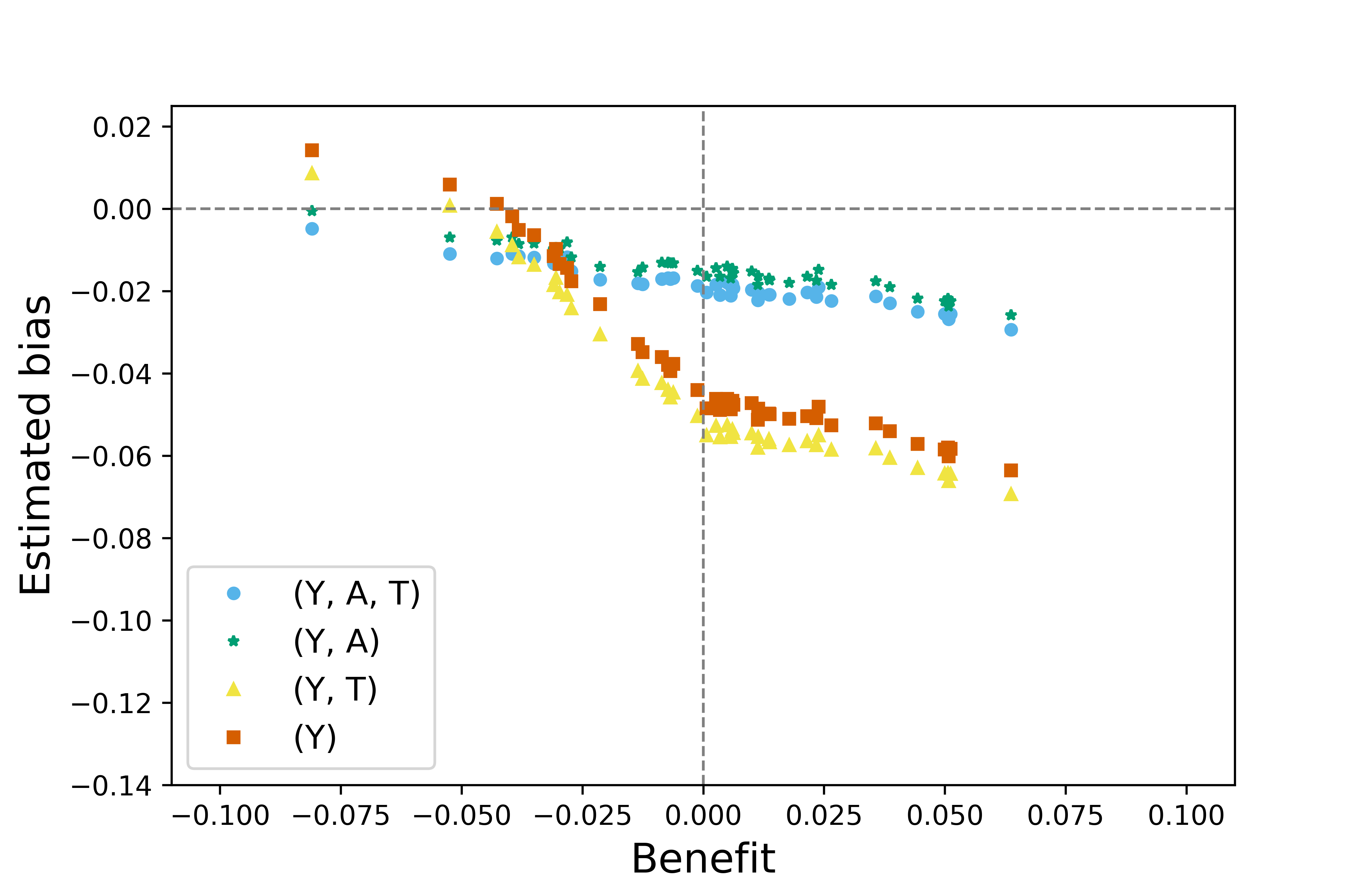
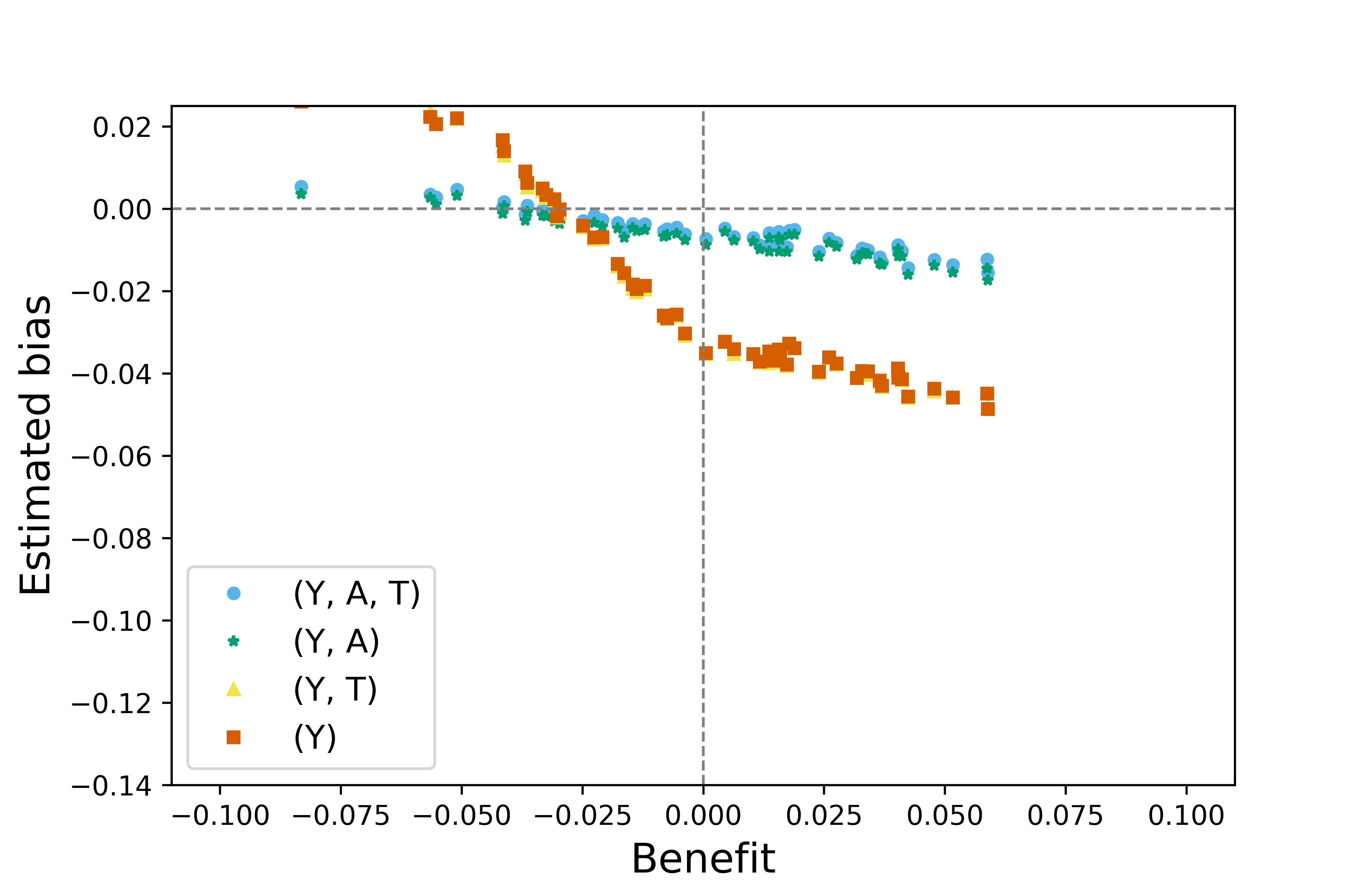
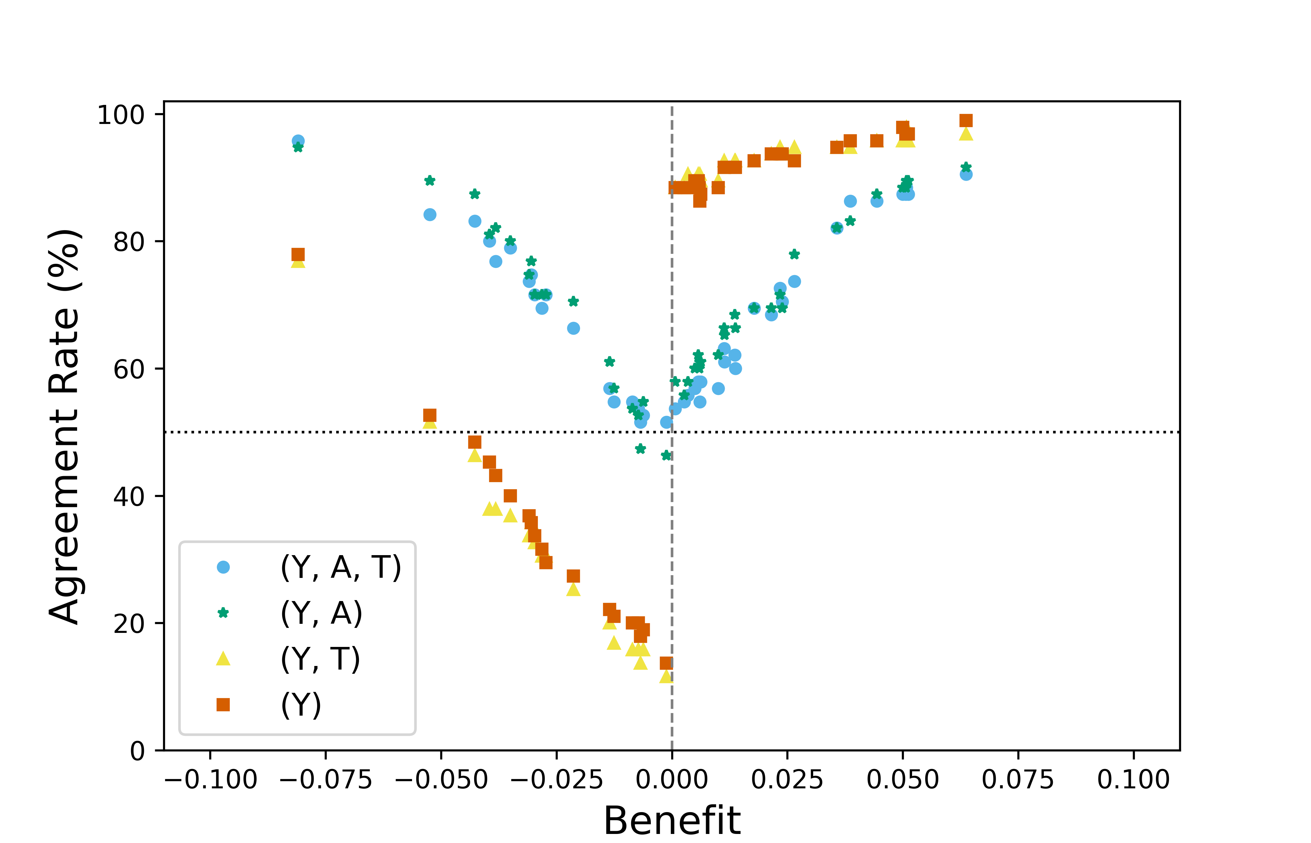
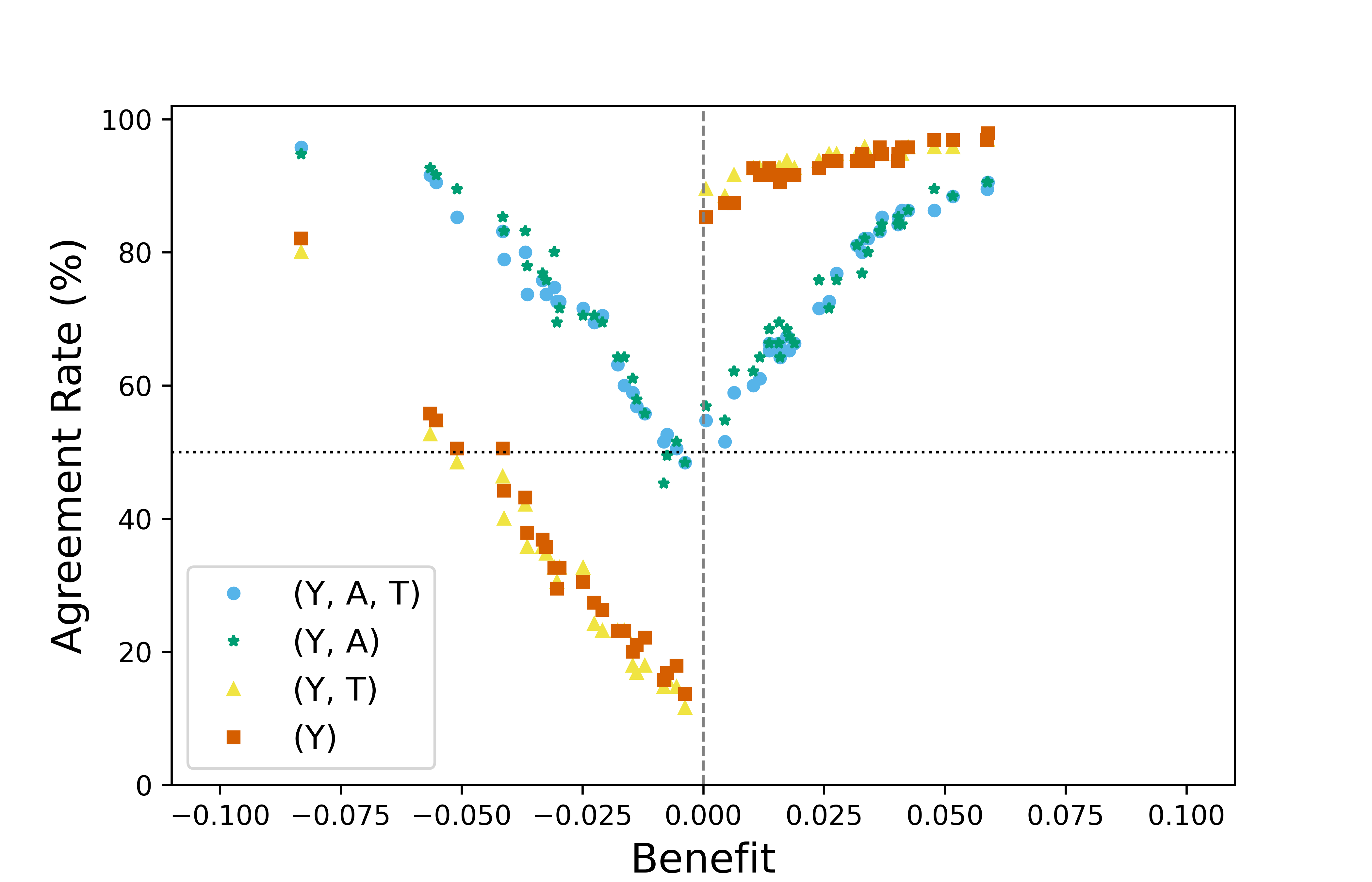
Figure 6: Benefit vs. estimated loss for all four model specifications given previous outcome – $y_{i1}=0$ (left) and $y_{i1}=1$ (right) – and data generated under $(u_{i,\mathrm{W}},u_{i,\mathrm{A}})\perp\!\!\!\perp u_{i,\mathrm{T}}.$

Figure 7: Benefit vs. agreement rate for all four model specifications given previous outcome – $y_{i1}=0$ (left) and $y_{i1}=1$ (right) – and data generated under $(u_{i,\mathrm{W}},u_{i,\mathrm{A}})\perp\!\!\!\perp u_{i,\mathrm{T}}.$

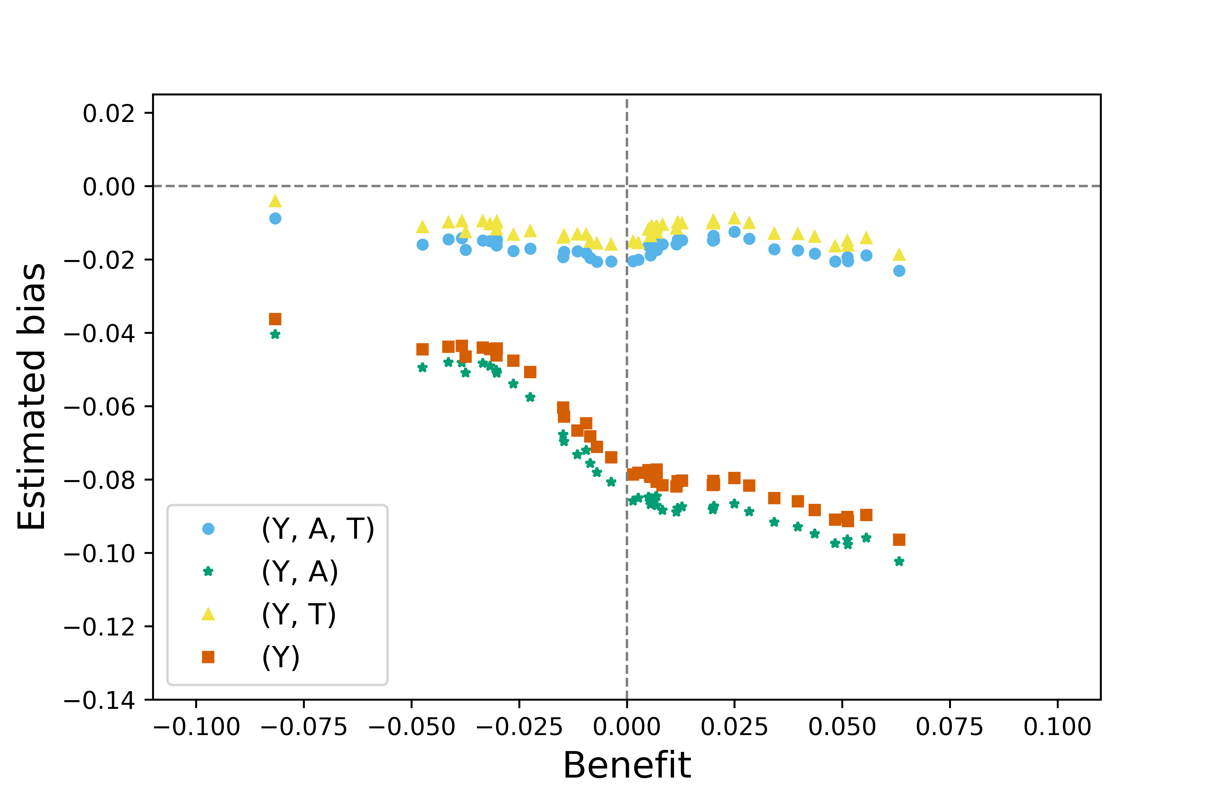
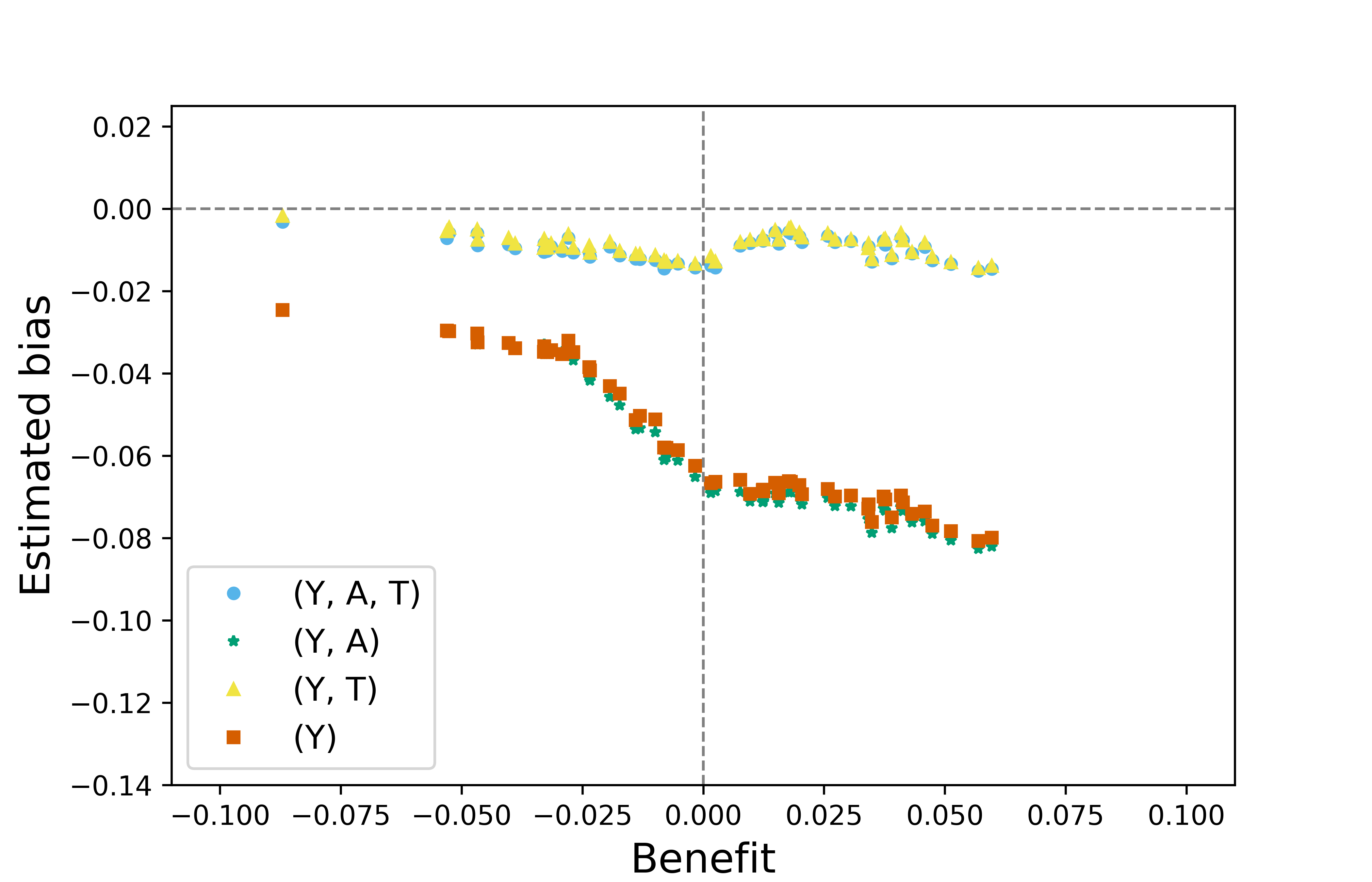
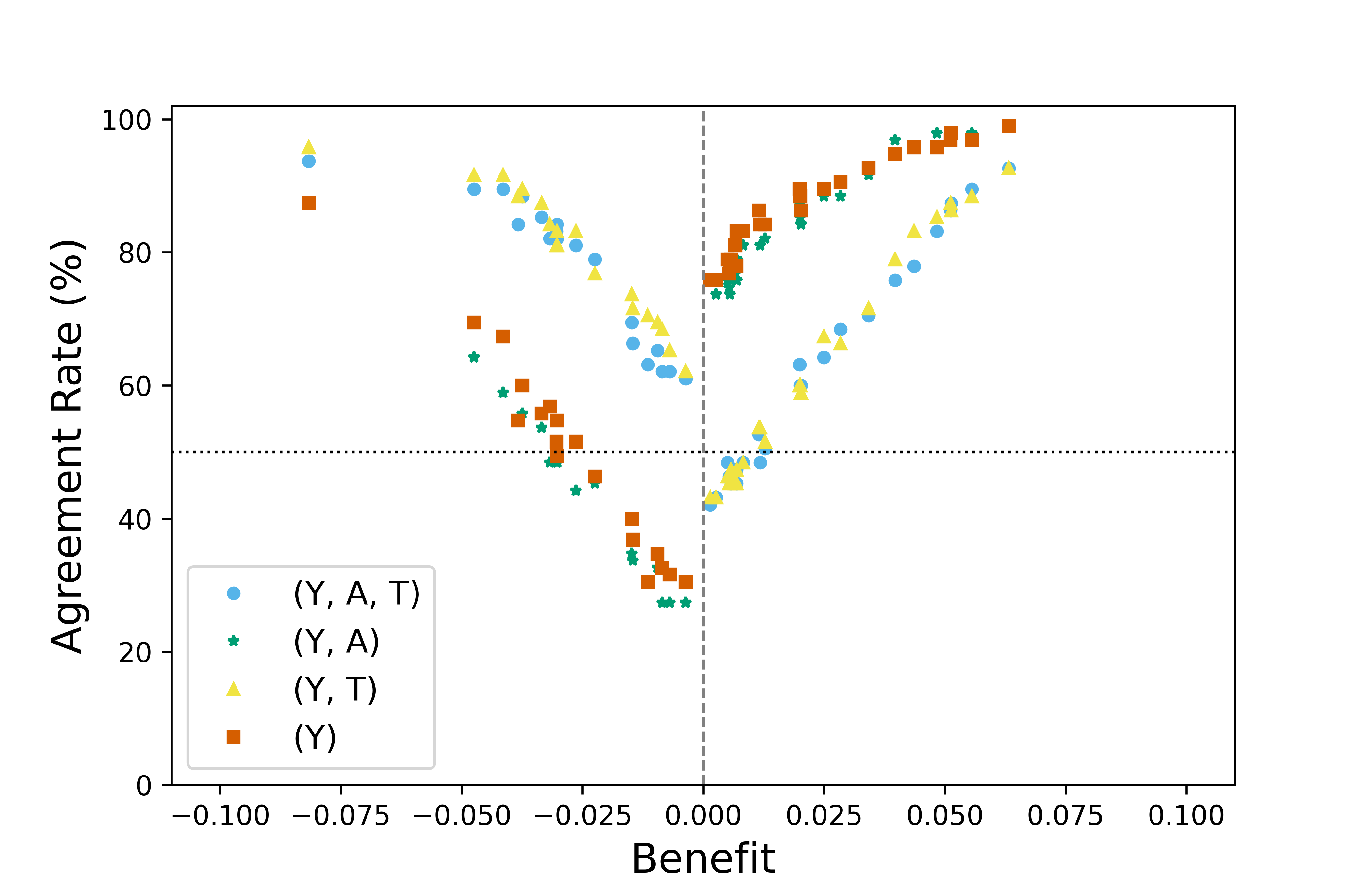
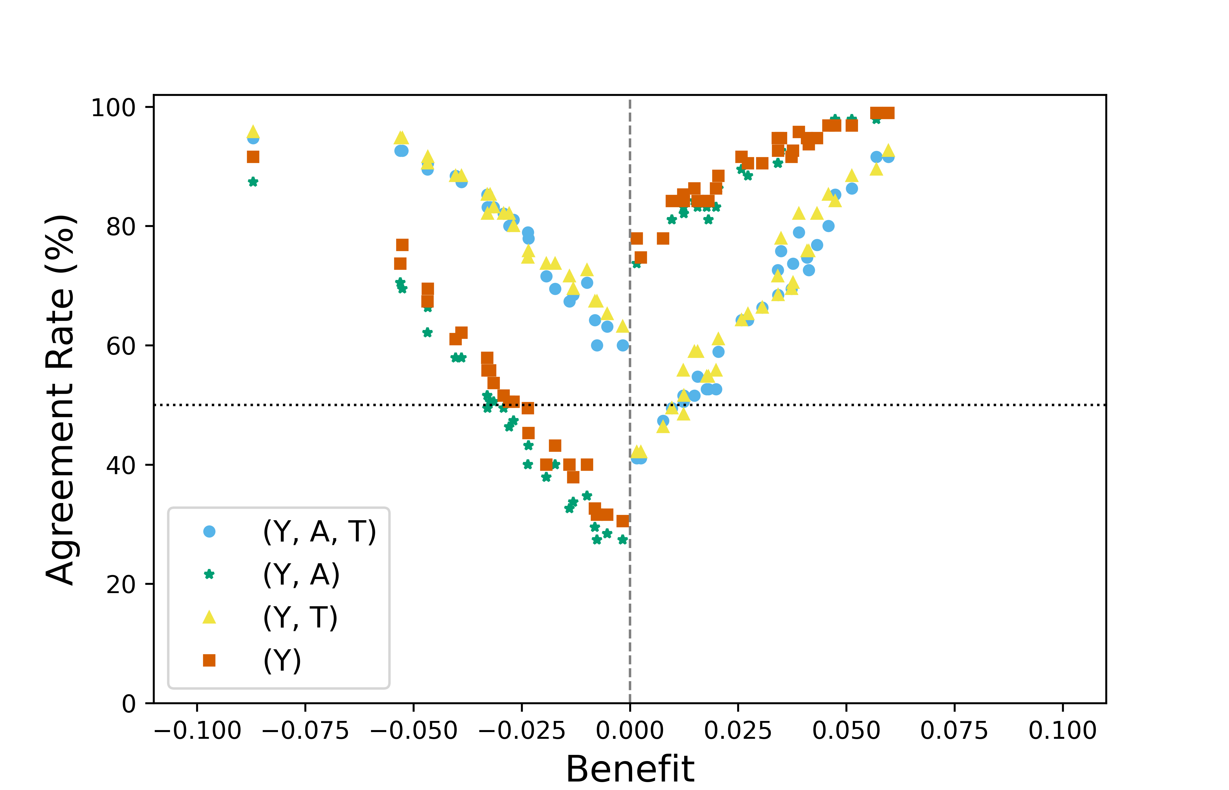
Figure 8: Benefit vs. estimated loss for all four model specifications given previous outcome – $y_{i1}=0$ (left) and $y_{i1}=1$ (right) – and data generated under $(u_{i,\mathrm{W}},u_{i,\mathrm{T}})\perp\!\!\!\perp u_{i,\mathrm{A}}.$

Figure 9: Benefit vs. agreement rate for all four model specifications given previous outcome – $y_{i1}=0$ (left) and $y_{i1}=1$ (right) – and data generated under $(u_{i,\mathrm{W}},u_{i,\mathrm{T}})\perp\!\!\!\perp u_{i,\mathrm{A}}.$

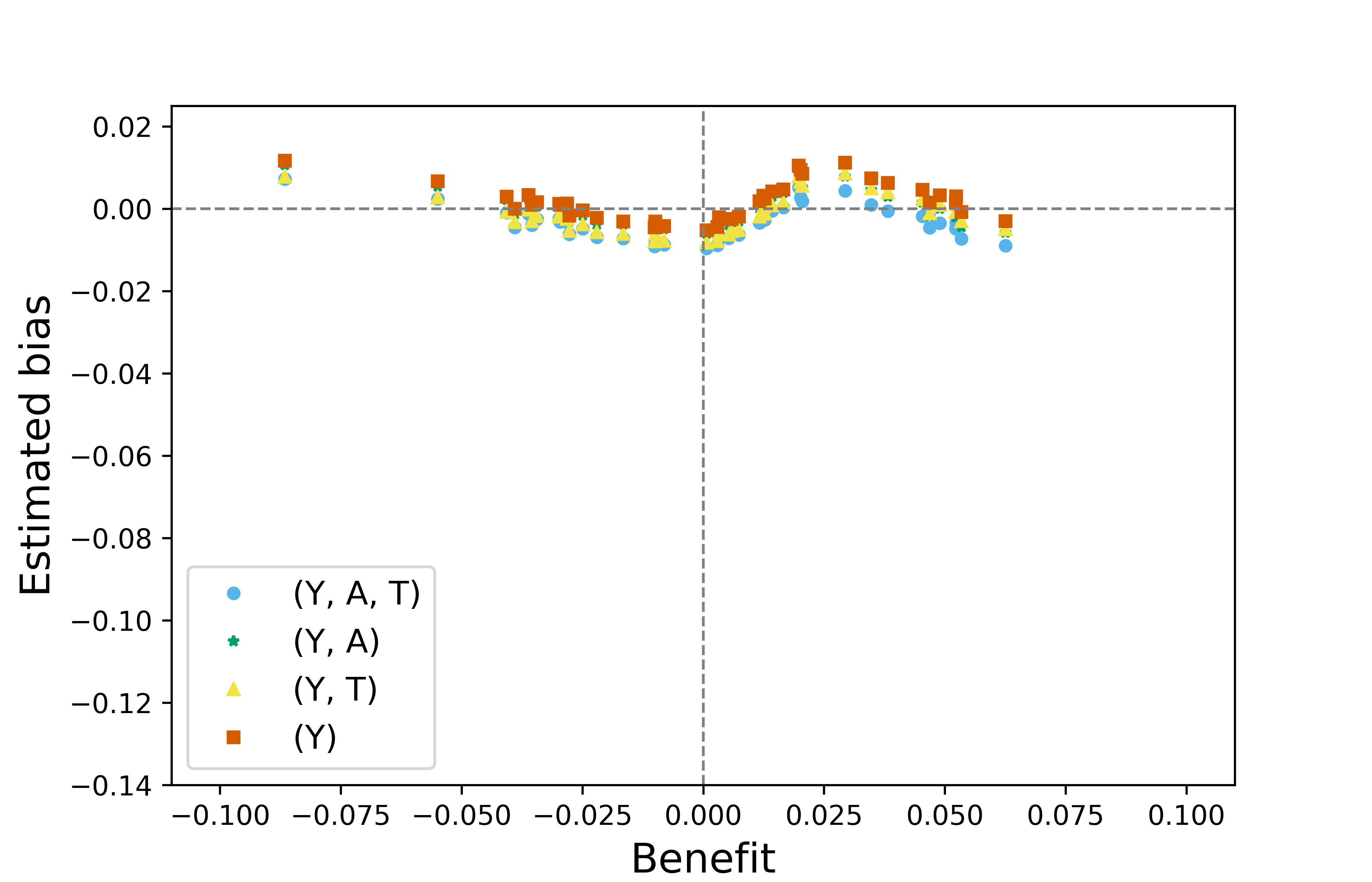
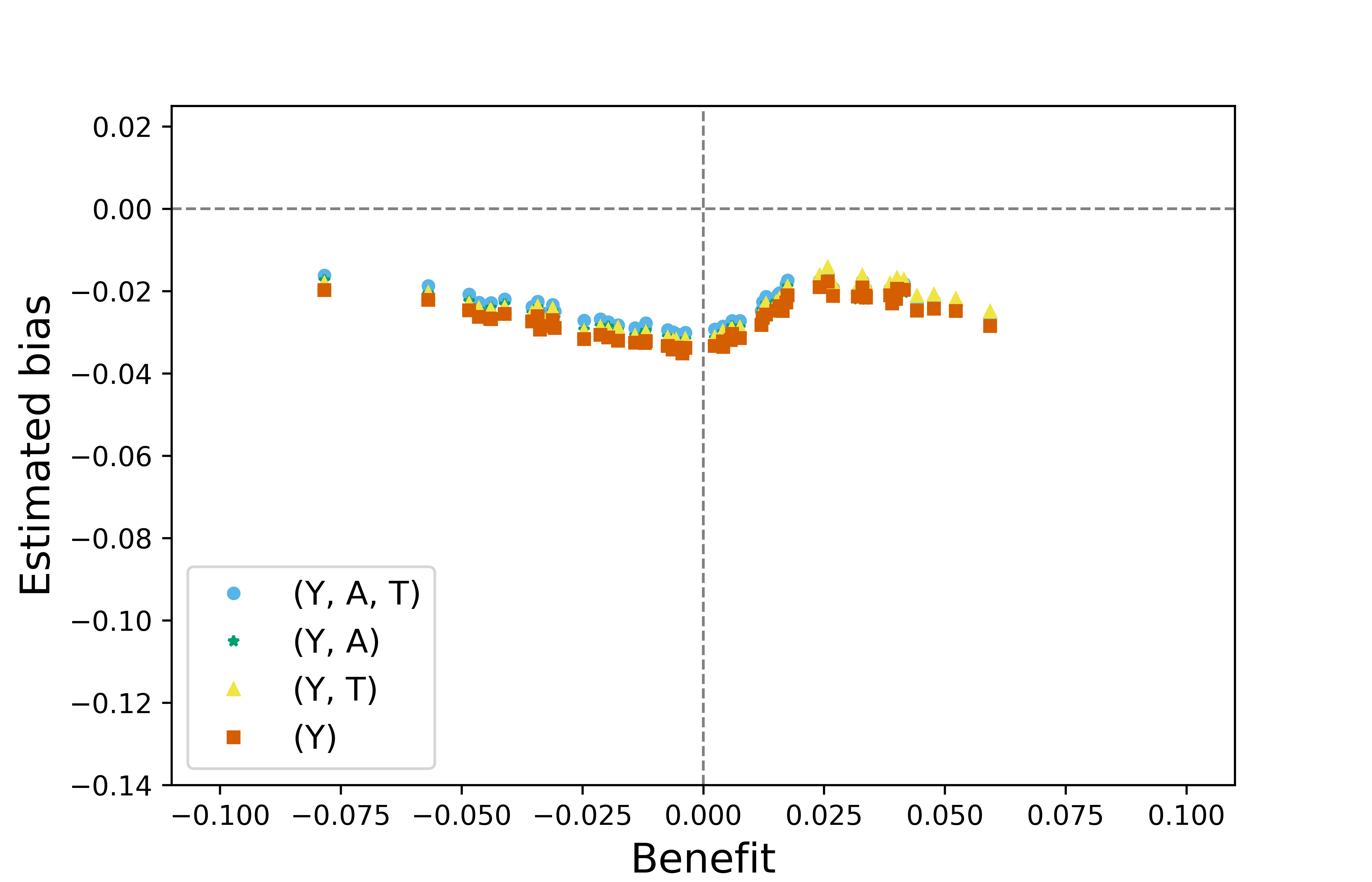
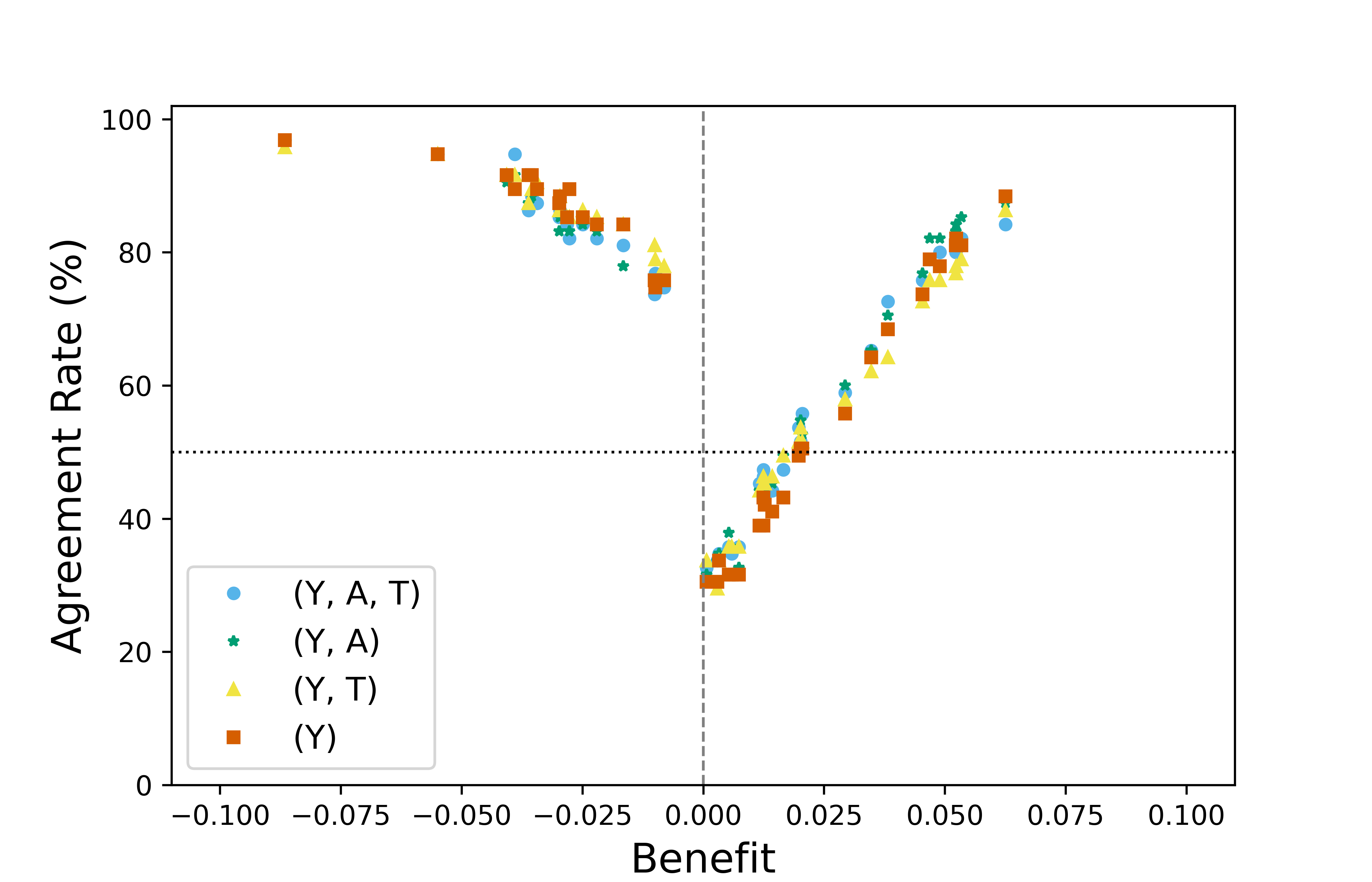
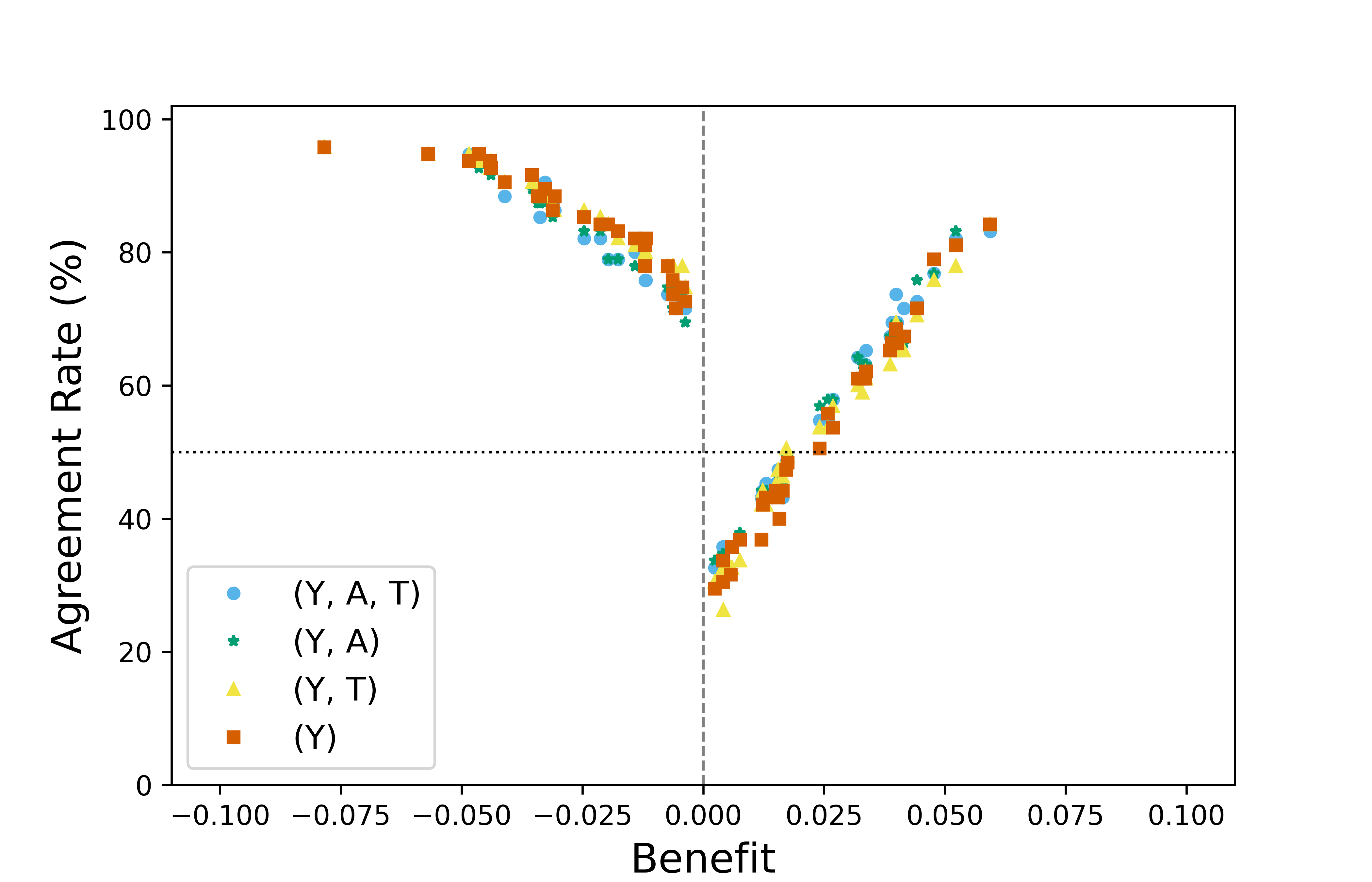
Figure 10: Benefit vs. estimated loss for all four model specifications given previous outcome – $y_{i1}=0$ (left) and $y_{i1}=1$ (right) – and data generated under $u_{i,\mathrm{W}}\perp\!\!\!\perp u_{i,\mathrm{A}}\perp\!\!\!\perp u_{i,\mathrm{T}}$.

Figure 11: Benefit vs. agreement rate for all four model specifications given previous outcome – $y_{i1}=0$ (left) and $y_{i1}=1$ (right) – and data generated under $u_{i,\mathrm{W}}\perp\!\!\!\perp u_{i,\mathrm{A}}\perp\!\!\!\perp u_{i,\mathrm{T}}$.

Appendix G Details on Data Analysis

G.1 Protocols of Original INSPIRE Studies and Target Trial

Protocol Component	INSPIRE 2 & 3 Protocols	Observational Setting	Target Trial Specification
Eligibility Criteria	HIV-infected adults on HAART	Idem	Idem
Treatment strategy	Three injections of IL-7 administered at 7-day intervals	One, two or three injections of IL-7 administered at 7-day intervals	Three injections of IL-7 administered at 7-day intervals
Treatment assignment	Provide IL-7 doses if CD4 blood concentration $\leqslant$ 550 cells/$\mu$L with a maximum of 4 injection cycles over 21 months of follow-up	0, 1, 2 or 3 injections were provided; when CD4 $\leqslant$ 550 cells/$\mu$L, at least one injection was often provided, but not always.	0 or 3 injections randomly provided, at 90-day intervals, with a maximum of three cycles across follow-up
Follow-up schedule	Quarterly intervals between assessments at which injections are decided to be administered or not	Some departure in protocol, both in the number of injections and scheduled visit time, can be observed.	Exactly 90-day intervals
Outcome	post-injection CD4 concentration	post-injection CD4 concentration	indicator of CD4 $\geqslant$ 500 cells/$\mu$L of blood
Target of inference	Time spent with CD4 blood concentration $\geqslant 500$ cells/$\mu$L	Idem	Conditional rewards under optimal regime

Table 5: Component-wise specifications of the INSPIRE 2 & 3 studies and the completely randomized SMART as $\mathcal{E}$ that we wish to emulate. Deviations from the INSPIRE protocol may result in confounding and informative visit time biases, rendering the data observational.

G.2 Frequency of Individualized Treatment Frequency

Treatment Course	Recommendation Frequency
$(0,1,0,0)$	67.9%
$(1,0,0,0)$	29.1%
$(0,0,1,0)$	3.0%

Table 6: Patient A individualized treatment recommendation.

Treatment course	Recommendation frequency
$(1,1,0,0)$	53.5%
$(1,0,1,0)$	33.8%
$(0,1,1,0)$	11.3%
$(0,1,0,1)$	0.6%
$(1,0,0,1)$	0.4%
$(0,0,1,1)$	0.3%

Table 7: Patient B individualized treatment recommendation.

G.3 MCMC Chains

Traceplots and empirical density plots for all four chains for reward parameters $\phi_{\mathrm{Y}}$, $\phi_{\mathrm{U}}$, $\mu$ and $\tau$ for the full joint model $(Y,A,T)$ are respectively displayed in Figures 12, 13 and 14 below.

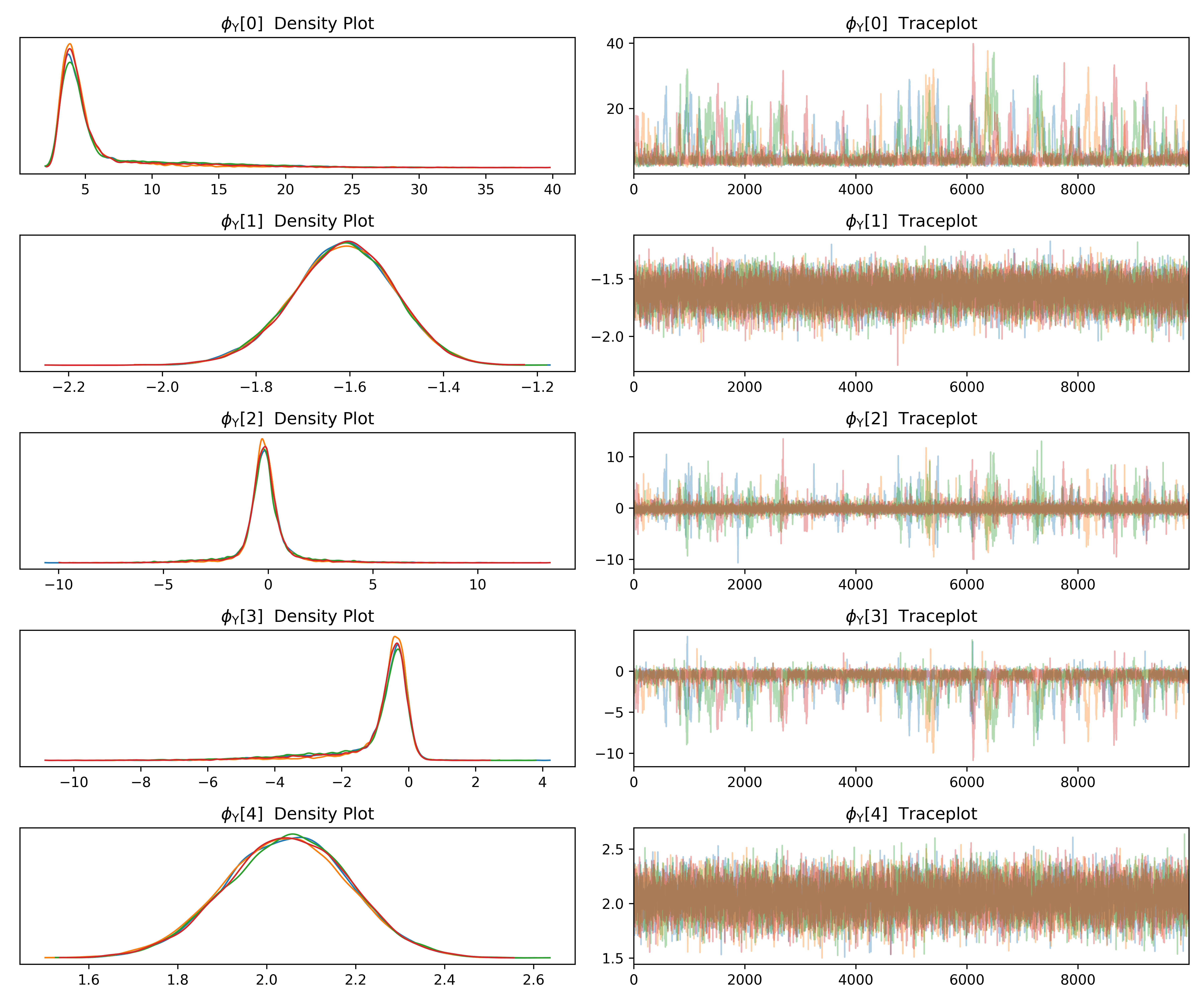
Figure 12: $\phi_{\mathrm{Y}}$ traceplots

Figure 13: $\phi_{\mathrm{U}}$ traceplots

Figure 14: $\mu$ and $\tau^{2}$ traceplots

G.4 Summary Table of Outcome Model Parameters

Coefficient	Estimate	95% Credible Interval
Intercept	–2.05	(–2.48, –1.70)
$A_{ij}^{\text{DR}}$	–3.41	(–2.83, –4.11)
$A_{ij}^{\text{DR}}*\operatorname{Age}_{i}$	–0.20	(–0.60, –0.21)
$A_{ij}^{\text{DR}}*\operatorname{BMI}_{i}$	–0.18	(–0.35, –0.16)
$A_{ij}^{\text{DR}}*Y_{i(j-1)}$	–1.48	(–1.24, –1.73)
$\mu$	–5.24	(–5.80, –4.68)
$\tau^{2}$	0.82	(–0.47, –1.64)

Table 8: Summary of outcome model parameters from MCMC.

	$\operatorname{Cov}(\cdot,U_{\mathrm{T}})$	$\operatorname{Cov}(\cdot,U_{\mathrm{A}})$	$\operatorname{Cov}(\cdot,U_{\mathrm{Y}})$
$\operatorname{Cov}(U_{\mathrm{T}},\cdot)$	–0.61 (–0.14, –4.11)	–0.01 (–2.43, –1.72)	–0.03 (–0.25, –0.42)
$\operatorname{Cov}(U_{\mathrm{A}},\cdot)$	–0.01 (–2.43, –1.72)	–0.70 (–0.14, –9.18)	–0.01 (–0.45, –0.45)
$\operatorname{Cov}(U_{\mathrm{Y}},\cdot)$	–0.03 (–0.25, –0.42)	–0.01 (–0.45, –0.45)	–0.17 (–0.08, –0.35)

Table 9: Summary of correlation matrix fit from MCMC.

References

- Coulombe et al. (2023) Coulombe, J., E. E. Moodie, S. M. Shortreed, and C. Renoux (2023). Estimating individualized treatment rules in longitudinal studies with covariate-driven observation times. Statistical Methods in Medical Research 32(5), 868–884.
- Davidian and Giltinan (2003) Davidian, M. and D. M. Giltinan (2003). Nonlinear models for repeated measurement data: an overview and update. Journal of Agricultural, Biological, and Environmental Statistics 8, 387–419.
- Dawid and Didelez (2010) Dawid, A. P. and V. Didelez (2010). Identifying the consequences of dynamic treatment strategies: A decision-theoretic overview. Statistics Surveys 4, 184 – 231.
- Dong et al. (2023) Dong, L., E. E. Moodie, L. Villain, and R. Thiébaut (2023). Evaluating the use of generalized dynamic weighted ordinary least squares for individualized HIV treatment strategies. The Annals of Applied Statistics 17, 2432–2451.
- Douek et al. (2009) Douek, D. C., M. Roederer, and R. A. Koup (2009). Emerging concepts in the immunopathogenesis of aids. Annual Review of Medicine 60(1), 471–484.
- Farewell et al. (2017) Farewell, D., C. Huang, and V. Didelez (2017). Ignorability for general longitudinal data. Biometrika 104(2), 317–326.
- Gasparini et al. (2020) Gasparini, A., K. R. Abrams, J. K. Barrett, R. W. Major, M. J. Sweeting, N. J. Brunskill, and M. J. Crowther (2020). Mixed-effects models for health care longitudinal data with an informative visiting process: A Monte Carlo simulation study. Statistica Neerlandica 74(1), 5–23.
- Guan et al. (2020) Guan, Q., B. J. Reich, E. B. Laber, and D. Bandyopadhyay (2020). Bayesian nonparametric policy search with application to periodontal recall intervals. Journal of the American Statistical Association 115(531), 1066–1078.
- Hernán (2011) Hernán, M. A. (2011). With great data comes great responsibility: publishing comparative effectiveness research in epidemiology. Epidemiology (Cambridge, Mass.) 22(3), 290.
- Hernán and Robins (2016) Hernán, M. A. and J. M. Robins (2016). Using big data to emulate a target trial when a randomized trial is not available. American Journal of Epidemiology 183(8), 758–764.
- Hernán and Robins (2020) Hernán, M. A. and J. M. Robins (2020). Causal inference: what if.
- Hernán et al. (2022) Hernán, M. A., W. Wang, and D. E. Leaf (2022). Target trial emulation: A framework for causal inference from observational data. JAMA 328(24), 2446–2447.
- Hoshino (2008) Hoshino, T. (2008). A Bayesian propensity score adjustment for latent variable modeling and MCMC algorithm. Computational Statistics & Data Analysis 52(3), 1413–1429.
- Hua et al. (2022) Hua, W., H. Mei, S. Zohar, M. Giral, and Y. Xu (2022). Personalized dynamic treatment regimes in continuous time: a Bayesian approach for optimizing clinical decisions with timing. Bayesian Analysis 17(3), 849–878.
- Keil et al. (2018) Keil, A. P., E. J. Daza, S. M. Engel, J. P. Buckley, and J. K. Edwards (2018). A Bayesian approach to the G-formula. Statistical Methods in Medical Research 27(10), 3183–3204.
- Lam et al. (2015) Lam, S. K., A. Pitrou, and S. Seibert (2015). Numba: A LLVM-based Python JIT compiler. In Proceedings of the Second Workshop on the LLVM Compiler Infrastructure in HPC, pp. 1–6.
- Lavori and Dawson (2000) Lavori, P. W. and R. Dawson (2000). A design for testing clinical strategies: biased adaptive within-subject randomization. Journal of the Royal Statistical Society: Series A (Statistics in Society) 163(1), 29–38.
- Lei et al. (2012) Lei, H., I. Nahum-Shani, K. Lynch, D. Oslin, and S. A. Murphy (2012). A “SMART” design for building individualized treatment sequences. Annual Review of Clinical Psychology 8, 21–48.
- Levy et al. (2009) Levy, Y., C. Lacabaratz, L. Weiss, J.-P. Viard, C. Goujard, J.-D. Lelièvre, F. Boué, J.-M. Molina, C. Rouzioux, V. Avettand-Fénoêl, et al. (2009). Enhanced T cell recovery in HIV-1–infected adults through IL-7 treatment. The Journal of Clinical Investigation 119(4), 997–1007.
- Moodie et al. (2007) Moodie, E. E., T. S. Richardson, and D. A. Stephens (2007). Demystifying optimal dynamic treatment regimes. Biometrics 63(2), 447–455.
- Murphy (2003) Murphy, S. A. (2003). Optimal dynamic treatment regimes. Journal of the Royal Statistical Society: Series B (Statistical Methodology) 65(2), 331–355.
- Oganisian et al. (2024) Oganisian, A., K. D. Getz, T. A. Alonzo, R. Aplenc, and J. A. Roy (2024). Bayesian semiparametric model for sequential treatment decisions with informative timing. Biostatistics 25, 947 – 961.
- Orihara et al. (2024) Orihara, S., S. Sugasawa, T. Ohigashi, T. Nakagawa, and M. Taguri (2024). Nonparametric bayesian adjustment of unmeasured confounders in cox proportional hazards models.
- Pullenayegum and Lim (2016) Pullenayegum, E. M. and L. S. Lim (2016). Longitudinal data subject to irregular observation: A review of methods with a focus on visit processes, assumptions, and study design. Statistical Methods in Medical Research 25(6), 2992–3014.
- Robins (2000) Robins, J. M. (2000). Marginal structural models versus structural nested models as tools for causal inference. In Statistical Models in Epidemiology, the Environment, and Clinical Trials, pp. 95–133. Springer.
- Ryu et al. (2007) Ryu, D., D. Sinha, B. Mallick, S. R. Lipsitz, and S. E. Lipshultz (2007). Longitudinal studies with outcome-dependent follow-up: models and Bayesian regression. Journal of the American Statistical Association 102(479), 952–961.
- Saarela et al. (2015) Saarela, O., E. Arjas, D. A. Stephens, and E. E. Moodie (2015). Predictive Bayesian inference and dynamic treatment regimes. Biometrical Journal 57(6), 941–958.
- Saarela et al. (2023) Saarela, O., D. A. Stephens, and E. E. Moodie (2023). The role of exchangeability in causal inference. Statistical Science 1(1), 1–17.
- Saarela et al. (2015) Saarela, O., D. A. Stephens, E. E. Moodie, and M. B. Klein (2015). On Bayesian estimation of marginal structural models. Biometrics 71(2), 279–288.
- Thiébaut et al. (2014) Thiébaut, R., J. Drylewicz, M. Prague, C. Lacabaratz, S. Beq, A. Jarne, T. Croughs, R.-P. Sekaly, M. M. Lederman, I. Sereti, et al. (2014). Quantifying and predicting the effect of exogenous Interleukin-7 on CD4+ T cells in HIV-1 infection. PLoS Computational Biology 10(5), e1003630.
- Thiébaut et al. (2016) Thiébaut, R., A. Jarne, J.-P. Routy, I. Sereti, M. Fischl, P. Ive, R. F. Speck, G. d’Offizi, S. Casari, D. Commenges, et al. (2016). Repeated cycles of recombinant human Interleukin 7 in HIV-infected patients with low CD4 T-cell reconstitution on antiretroviral therapy: results of 2 phase II multicenter studies. Clinical Infectious Diseases 62(9), 1178–1185.
- Tsiatis et al. (2019) Tsiatis, A. A., M. Davidian, S. T. Holloway, and E. B. Laber (2019). Dynamic treatment regimes: Statistical methods for precision medicine. CRC press.
- Villain et al. (2019) Villain, L., D. Commenges, C. Pasin, M. Prague, and R. Thiébaut (2019). Adaptive protocols based on predictions from a mechanistic model of the effect of IL7 on CD4 counts. Statistics in Medicine 38(2), 221–235.
- Wallace et al. (2016) Wallace, M. P., E. E. Moodie, and D. A. Stephens (2016). Smart thinking: a review of recent developments in sequential multiple assignment randomized trials. Current Epidemiology Reports 3, 225–232.
- Yiu et al. (2022) Yiu, A., E. Fong, S. Walker, and C. Holmes (2022). Causal predictive inference and target trial emulation.
- Zeger and Liang (1986) Zeger, S. L. and K.-Y. Liang (1986). Longitudinal data analysis for discrete and continuous outcomes. Biometrics 42(1), 121–130.