Parameter Tracking in Federated Learning with Adaptive Optimization

Abstract

In Federated Learning (FL), model training performance is strongly impacted by data heterogeneity across clients. Gradient Tracking (GT) has recently emerged as a solution which mitigates this issue by introducing correction terms to local model updates. To date, GT has only been considered under Stochastic Gradient Descent (SGD)-based model training, while modern FL frameworks increasingly employ adaptive optimizers for improved convergence. In this work, we generalize the GT framework to a more flexible Parameter Tracking (PT) paradigm and propose two novel adaptive optimization algorithms, FAdamET and FAdamGT, that integrate PT into Adam-based FL. We provide a rigorous convergence analysis of these algorithms under non-convex settings. Our experimental results demonstrate that both proposed algorithms consistently outperform existing methods when evaluating total communication cost and total computation cost across varying levels of data heterogeneity, showing the effectiveness of correcting first-order information in federated adaptive optimization.

1 Introduction

Federated Learning (FL) has emerged as a promising paradigm for training Machine Learning (ML) models across distributed devices [17, 10]. Migitating data heterogeneity remains one of the most critical challenges in FL. This non-i.i.d. characteristic of client data often results in slower convergence and suboptimal model performance. While traditional Stochastic Gradient Descent (SGD)-based optimizers are widely employed in FL frameworks, they exhibit limited effectiveness in addressing the adverse effects of heterogeneous data [24]. To overcome these limitations, the concept of Gradient Tracking (GT) has been introduced [5]. GT incorporates correction terms during communication, enabling clients to locally estimate and compensate for the gradient contributions from other clients in the network. This approach helps mitigate the negative impacts of data heterogeneity, thereby improving the convergence behavior and stability of the global model.

Beyond the widely used SGD optimizer, moment-based optimizers have emerged as prominent local update schemes for ML training [6, 9, 12]. Numerous algorithms have been proposed, and these adaptive optimizers have demonstrated superior empirical performance compared to SGD. Efforts have been made to integrate adaptive optimizers into FL frameworks; however, these approaches often suffer from performance degradation in the presence of data heterogeneity, especially when communication cost is high and cannot be performed frequently. Existing research leveraging GT to address data heterogeneity in FL primarily focuses on SGD optimizers. Consequently, since most adaptive optimization algorithms involves multiplying and dividing gradient-based estimates, how to effectively track first-order gradient information remains a challenging task.

Motivated by this, we investigate the following questions:

1. Will adaptive optimization algorithms designed using GT obtain performance advantages across FL systems as their SGD counterparts?

2. What is the best way to incorporate the concept of GT into adaptive federated optimization?

In answering these questions, we extend the concept of GT to a more generalized framework termed Parameter Tracking (PT). Building upon this foundation, we propose two novel algorithms leveraging the Adaptive Moment Estimation (Adam) optimizer. Through rigorous convergence analysis and comprehensive experimental evaluations, we demonstrate that both algorithms effectively stabilize the global learning process. As a result, increasing levels of non-i.i.d. data distributions across clients do not readily lead to a decline in performance, addressing a critical limitation in existing federated optimization techniques.

Our main contributions are as follows:

• We introduce a generalized concept of GT termed Parameter Tracking (PT), where local clients track the discrepancy between their locally collected first-order information and the server’s aggregated information (Sec. 4.1). This extension proves beneficial when integrating the Adam optimizer into FL.

• Base on the concept of PT, we propose two novel Adam-based algorithms, FAdamET and FAdamGT, by leveraging different interpretations of PT. Both approaches effectively track global information by using control variables that does not require any additional fine-tuning, mitigating model biases caused by various levels of non-i.i.d. data efficiently (Sec. 4.2 and 4.3).

• We provide a rigorous theoretical analysis of the convergence rates for both algorithms. This offers insights into their stability and efficiency under heterogeneous data conditions, and better understanding of how PT works differently when applied to different steps of the local update process (Sec. 5.2).

• We perform extensive experiments across diverse datasets and multiple FL settings, including image classification tasks using convolution neural networks (CNN) and sequence classification tasks using large language models (LLMs), demonstrating the superior performance of our proposed methods compared to existing baselines (Sec. 6).

2 Related Works

Gradient Tracking: Gradient Tracking (GT) methods [5, 21, 27, 13, 3, 26, 29] have emerged as a powerful solution to address data heterogeneity challenges in decentralized optimization algorithms. The core principle of GT lies in tracking gradient information from neighboring nodes during each communication round, ensuring more accurate gradient estimates across the network. Centralized FL algorithms such as SCAFFOLD [11] and Proxskip [20] are both designed base on this concept, and multiple works on serverless FL settings demonstrated superior improvement [18, 8, 2, 1], where communication efficiency is a primary concern. By effectively reducing the synchronization frequency while still guaranteeing convergence to the optimal point, GT has proven to be highly effective in mitigating the adverse effects of heterogeneous data distributions. Furthermore, existing studies have shown that under proper initialization of gradient tracking variables, many standard assumptions on data heterogeneity can be relaxed.

Recent advancements have also extended GT methods to address hierarchical network structures. SDGT was introduced as the first GT algorithm tailored for semi-decentralized networks [4], bridging the gap between fully decentralized and centralized topologies. Meanwhile, [7] proposed MTGC, a multi-timescale GT algorithm capable of operating efficiently in multi-tier networks. Despite these advancements, existing works predominantly focus on designing SGD based algorithms, leaving the combination of GT and adaptive optimizers largely unexplored and an open challenge.

Adaptive Optimizer: SGD optimizers rely on fixed or decaying learning rates, which often require careful tuning and may struggle with scenarios involving sparse gradients or noisy updates. To address these limitations, adaptive optimizers dynamically adjust learning rates based on the gradient history of individual parameters, enabling more effective navigation of complex optimization landscapes. Among the most prominent adaptive optimizers are AdaGrad [6], and Adam [12]. AdaGrad introduces per-parameter learning rate scaling to handle sparse features effectively. Building on this foundation, Adam combines the benefits of momentum with adaptive learning rates, achieving robust convergence across various learning tasks. Recent advancements have further explored the decoupling of weight decay [19] and the time-varying effects of regularization terms [31], pushing the boundaries of adaptive optimization.

Several approaches have been proposed to integrate adaptive optimizers into FL. [23] introduced FedAdam, where the central server employs an adaptive optimizer to update the global model using aggregated client gradients. Additionally, [30] incorporates adaptive optimization directly on local clients. More recently, [25] presented FedLADA, an FL algorithm in which clients utilize the Adam optimizer for local updates. In FedLADA, the update gradient is computed as a weighted average of local gradients and global gradients. However, besides FedLADA, all of these algorithms aren’t designed to deal with data heterogeneity, and hence requires frequent global aggregation for good results. FedLADA although maintained a global gradient estimation, requires a weighted sum operation where an additional hyperparameter has to be fine-tuned based on different data. This causes the performance to vary dramatically base on the chosen weights, which is not required in our algorithms.

3 System Model and Motivation

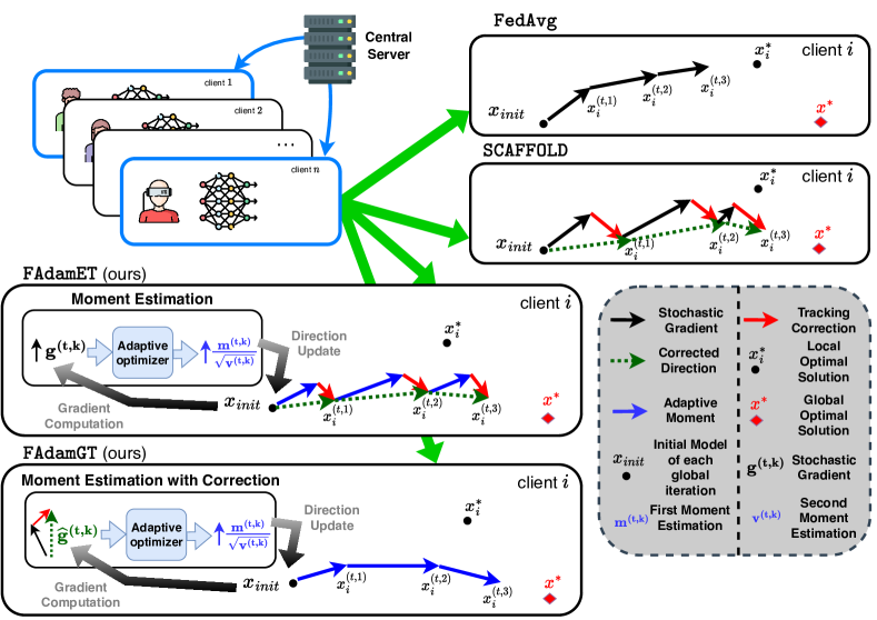
Figure 1: Visualization of the local update process of multiple federated learning algorithms. Whereas SCAFFOLD adds correction terms into the SGD update of FedAvg, our methods, FAdamET and FAdamGT, incorporate PT correction terms into local updates based on adaptive optimization updates. FAdamET injects correction terms after computing adaptive estimated moments, and FAdamGT injects correction terms before computing adaptive estimated moments.

3.1 System Model

The problem we aim to solve follows the form:

$$\textstyle\min_{x\in\mathbb{R}^{d}}f(x) \textstyle=\frac{1}{n}\sum_{i=1}^{n}f_{i}(x),$$ (1)

where $f_{i}(x)=\mathbb{E}_{\xi_{i}\sim\mathcal{D}_{i}}f_{i}(x;\xi_{i})$ is the expectation of the stochastic local function, and $n$ is the total number of clients (typically edge devices) in the system, indexed $i=1,\ldots,n$. $f_{i}(x)$ is the local ML loss function computed at client $i$ for model parameters $x\in\mathbb{R}^{d}$, $\mathcal{D}_{i}$ is the local data distribution at client $i$, and $\xi_{i}$ is an unbiased random sample from $\mathcal{D}_{i}$. The server is connected to each device over a star topology, hence allowing the server to have direct communication between any device in the network.

The training process operates on two distinct timescales: an outer timescale and an inner timescale. The outer timescale, denoted as $t=1,2,\ldots,T$, represents global aggregation rounds where the central server updates the global model. The inner timescale, denoted as $k=1,\ldots,K$, represents local training steps performed by each client between global aggregations. We assume a fixed number of $K$ local updates occur between two consecutive global aggregation rounds.

For each global iteration $t$, the training procedure can be described in three iterative steps: (i) Client Selection and Initialization: At each global round $t$, the server selects a subset of clients $\mathcal{S}^{t}\subseteq\{1,\ldots,n\}$, where $|\mathcal{S}^{t}|=S\leq n$. The global model is broadcasted to the selected clients to initialize local training. (ii) Local Model Updates: Each selected client performs $K$ local updates using a local optimizer, independently updating their local models based on their respective datasets. (iii) Global Model Aggregation: After completing $K$ local updates, the selected clients send their updated model parameters to the server. The server then aggregates these updates to refine the global model.

3.2 Limitation of Existing Works

Federated adaptive algorithms such as LocalAdam exhibit instability under data heterogeneity, similar to FedAvg. Specifically, the local update does not remain stable at the optimal solution. Let $m_{i}=m^{*}=\nabla f(x^{*})=0$, $v_{i}=v^{*}=\nabla f(x^{*})\odot\nabla f(x^{*})$, and $x_{i}=x^{*}$. A single local update on client $i$ at the optimal point can be expressed as:

$$\textstyle m_{i}^{+} \textstyle=\beta_{1}m^{*}+(1-\beta_{1})\nabla f_{i}(x^{*}),$$

$$\textstyle v_{i}^{+} \textstyle=\beta_{2}v^{*}+(1-\beta_{2})\nabla f_{i}(x^{*})\odot\nabla f_{i}(x^{*}),$$

$$x_{i}^{+} \textstyle=x_{i}-\eta\frac{m_{i}^{+}}{\sqrt{v_{i}^{+}}+\epsilon}\neq x^{*}.$$ (LocalAdam)

This discrepancy between $x_{i}^{+}$ and $x^{*}$ implies that LocalAdam only converges to a region around the stationary point, where the radius depends on the degree of data heterogeneity.

To aim to address this issue, FedLADA introduces a weighted-average update, where a global averaged term $g_{\alpha}$ is calculated by the server and broadcasted to all sampled clients. The ideal value of $g_{\alpha}$ is $g_{\alpha}^{*}=\frac{m^{*}}{\sqrt{v^{*}}+\epsilon}$. However, even with the additional weighted-average operation, the ideal update of FedLADA still remains unstable:

$$\textstyle m_{i}^{+} \textstyle=\beta_{1}m^{*}+(1-\beta_{1})\nabla f_{i}(x^{*}),$$

$$\textstyle v_{i}^{+} \textstyle=\beta_{2}v^{*}+(1-\beta_{2})\nabla f_{i}(x^{*})\odot\nabla f_{i}(x^{*}),$$

$$x_{i}^{+} \textstyle=x_{i}-\eta\left(\alpha\frac{m_{i}^{+}}{\sqrt{v_{i}^{+}}+\epsilon}+(1-\alpha)g_{\alpha}^{*}\right).$$ (FedLADA)

The iterates are still unstable, since for any $\alpha\in(0,1]$, $x_{i}^{+}\neq x^{*}$. The equality only holds when $\alpha=0$, indicating that no local gradients are utilized during local updates, which is a trivial and impractical solution for mitigating data heterogeneity effectively.

4 Proposed Algorithm

The usage of PT correction is shown in Figure 1, where we show two possible locations when correction terms can participate into the local update: before the moment estimation and after the moment estimation.

4.1 Model Correction with First-order Information

GT has significantly improved the performance of SGD methods. We generalize GT to Parameter Tracking, where the core principle remains to locally track first-order update information, but it is not strictly limited to gradient information. This generalization aims to make FL with all kinds of local optimizer more resilient to data heterogeneity.

Adam optimizer employs multiple variables to track first-order information. With parameter tracking, these variables can be adapted at various stages of the algorithm, enabling the derivation of novel FL algorithms. In this paper, we propose two such algorithms, building upon LocalAdam [25] as a baseline, which replaces the local SGD optimizer in FedAvg with an Adam optimizer.

Case 1: Estimate Correction with Parameter Tracking. For a given local iteration, the local Adam optimizer performs updates as follows:

$$m_{i}^{+} \textstyle=\beta_{1}m_{i}+(1-\beta_{1})g_{i},$$

$$v_{i}^{+} \textstyle=\beta_{2}v_{i}+(1-\beta_{2})g_{i}\odot g_{i},$$

$$x_{i}^{+} \textstyle=x_{i}-\eta\frac{m_{i}^{+}}{\sqrt{v_{i}^{+}}+\epsilon},$$ (2)

where $m_{i}$ and $v_{i}$ represent first and second moment estimates, and $\epsilon$ ensures numerical stability. In an ideal communication scenario where server synchronization occurs at every local step, the server update can be expressed as:

$$\textstyle x^{+}=x-\eta\sum_{i=1}^{n}\frac{m_{i}^{+}}{\sqrt{v_{i}^{+}}+\epsilon}.$$

The objective of parameter tracking is to correct the discrepancy between the server and local updates via an ideal correction term:

$$\textstyle z_{\textrm{ideal}}=\sum_{i=1}^{n}\frac{m_{i}^{+}}{\sqrt{v_{i}^{+}}+\epsilon}-\frac{m_{i}^{+}}{\sqrt{v_{i}^{+}}+\epsilon}.$$

As shown in Figure 1, the corrected local update now becomes:

$$\textstyle x_{i}^{+}=x_{i}-\eta\left(\frac{m_{i}^{+}}{\sqrt{v_{i}^{+}}+\epsilon}+z_{\textrm{ideal}}\right)=x^{+}.$$

This adjustment ensures that local updates better approximate globally synchronized updates.

Case 2: Gradient Correction with Parameter Tracking.

Instead of emulating LocalAdam with per-iteration communication, we now start from the setting where the server applies Adam updates onto the global model using aggregated gradients from local clients. Based on (2), the ideal server-side update can be given as:

$$m^{+} =\textstyle\beta_{1}m+(1-\beta_{1})\sum_{i=1}^{n}g_{i},$$

$$v^{+} =\textstyle\beta_{2}v+(1-\beta_{2})\sum_{i=1}^{n}g_{i}\odot\sum_{i=1}^{n}g_{i},$$

$$x^{+} =\textstyle x-\eta\frac{m^{+}}{\sqrt{v^{+}}+\epsilon}.$$ (3)

The correction term here thus accounts for the difference between aggregated gradients and local gradients:

$$\textstyle z_{\textrm{ideal}}=\sum_{i=1}^{n}g_{i}-g_{i}.$$

As shown in Figure 1, by incorporating this correction term, the local updates are refined as:

$$m_{i}^{+} \textstyle=\beta_{1}m_{i}+(1-\beta_{1})(g_{i}+z_{\textrm{ideal}}),$$

$$v_{i}^{+} \textstyle=\beta_{2}v_{i}+(1-\beta_{2})(g_{i}+z_{\textrm{ideal}})\odot(g_{i}+z_{\textrm{ideal}}),$$

$$x_{i}^{+} \textstyle=x_{i}-\eta\left(\frac{m_{i}^{+}}{\sqrt{v_{i}^{+}}+\epsilon}\right)\approx x^{+}.$$

This formulation ensures that local updates align closely with the server updates in (4.1), and if $m_{i}=m,\forall i$ and $v_{i}=v,\forall i$, we get $x_{i}^{+}=x^{+}$.

4.2 Estimate Tracking

Based on Case 1 of Sec. 4.1, we propose Federated Adaptive Moment Estimation with Estimate Tracking (FAdamET), where we incorporate the concept of PT into LocalAdam. As shown in Algorithm 1, during each global iteration $t$, the server samples a set of clients $\mathcal{S}^{t}$ with size $S$ for training, and a smaller subset of clients $\mathcal{Y}^{t}\subseteq\mathcal{S}^{t}$ with size $Y$ that will perform update on the tracking terms. Further experimental results shows that choosing $Y\leq S$ can still obtain comparable results while saving total communication.

During the start of each local training interval, the server broadcasts the global model $x^{(t)}$ and the global correction term $y^{(t)}$ to all sampled clients $\mathcal{S}^{t}$. Then, for each sampled client $i$ at local iteration $k$, stochastic gradient $g_{i}^{(t,k)}=\nabla f_{i}(x_{i}^{(t,k)},\xi_{i}^{(t,k)})$ is computed locally using the local model $x_{i}^{(t,k)}$. The adaptive local update direction $\Delta_{i}^{(t,k)}$ then calculated using $g_{i}^{(t,k)}$. In this work, we use the Adam optimizer as shown in line 13-16 of Algorithm 1, but it is possible for a more general framework where other adaptive optimizers are considered. Then, the local model performs one update using the PT correction terms and the local update direction:

$$x_{i}^{(t,k+1)}=x_{i}^{(t,k)}-\eta_{l}(\Delta_{i}^{(t,k)}+y^{(t)}-y_{i}^{(t)}).$$

After $K$ local updates, all clients in $\mathcal{S}^{t}$ aggregated its local model to the server to update the global model $x^{(t)}$, and all clients in $\mathcal{Y}^{t}$ updates locally its PT correction terms and aggregate them to the server to update the server’s correction term $y^{(t)}$.

Algorithm 1 FAdamET and FAdamGT

1: Input: Global aggregations $T$, minibatch size, $|\xi_{i}^{(t,k)}|$, initial global model $x^{(1)}$

2: Output: Global model $x^{(T+1)}$

3: for $t=1$ to $T$ do

4:  randomly sample clients $\mathcal{S}^{t}\subseteq\{1,\ldots,n\}$.

5:  randomly sample clients for update tracking terms $\mathcal{Y}^{t}\subseteq\mathcal{S}^{t}$

6:  server broadcasts $(x^{(t)},y^{(t)})$ to all clients $i\in\mathcal{S}^{t}$

7:  for clients $i\in\mathcal{S}^{t}$ in parallel do

8:   initialize: $x_{i}^{(t,1)}=x^{(t)}$, $m_{i}^{(t,1)}=0$, $v_{i}^{(t,1)}=v_{i}^{(t)}$

9:   for $k=1$ to $K$ do

10:    compute mini-batch gradient $g_{i}^{(t,k)}$

11:    $\hat{g}_{i}^{(t,k)}=g_{i}^{(t,k)}$ (FAdamET)

12:    $\hat{g}_{i}^{(t,k)}=g_{i}^{(t,k)}+y^{(t)}-y_{i}^{(t)}$ (FAdamGT)

13:    $m_{i}^{(t,k+1)}=\beta_{1}m_{i}^{(t,k)}+(1-\beta_{1})\hat{g}_{i}^{(t,k)}$

14:    $v_{i}^{(t,k+1)}=\beta_{2}v_{i}^{(t,k)}+(1-\beta_{2})\hat{g}_{i}^{(t,k)}\odot\hat{g}_{i}^{(t,k)}$

15:    $\hat{v}_{i}^{(t,k+1)}=\max(\hat{v}_{i}^{(t,k)},v_{i}^{(t,k+1)})$

16:    $\Delta_{i}^{(t,k)}=m_{i}^{(t,k+1)}/(\sqrt{\hat{v}_{i}^{(t,k+1)}}+\epsilon)$

17:    $x_{i}^{(t,k+1)}=x_{i}^{(t,k)}-\eta_{l}(\Delta_{i}^{(t,k)}+y^{(t)}-y_{i}^{(t)})$ (FAdamET)

18:    $x_{i}^{(t,k+1)}=x_{i}^{(t,k)}-\eta_{l}\Delta_{i}^{(t,k)}$ (FAdamGT)

19:   end for

20:   if  $i\in\mathcal{Y}^{t}$ then

21:    $y_{i}^{(t+1)}=y_{i}^{(t)}-y^{(t)}+\frac{1}{K\eta_{l}}(x^{(t)}-x_{i}^{(t,K+1)})$ (FAdamET)

22:    $y_{i}^{(t+1)}=\frac{1}{K}\sum_{k=1}^{K}g_{i}^{(t,k)}$ (FAdamGT)

23:   end if

24:   $v_{i}^{(t+1)}=v_{i}^{(t,K+1)}$

25:  end for

26:  Server aggregates $x_{i}^{(t,K+1)}-x^{(t)}$ from clients $i\in\mathcal{S}^{t}$.

27:  Server aggregates $y_{i}^{(t+1)}-y_{i}^{(t)}$ from clients $i\in\mathcal{Y}^{t}$.

28:  $x^{(t+1)}=x^{(t)}+\eta_{g}\frac{1}{S}\sum_{i\in\mathcal{S}^{t}}(x_{i}^{(t,K+1)}-x^{(t)})$.

29:  $y^{(t+1)}=y^{(t)}+\frac{1}{n}\sum_{i\in\mathcal{Y}^{t}}(y_{i}^{(t+1)}-y_{i}^{(t)})$

30: end for

4.3 Gradient Tracking

Based on Case 2 of Sec. 4.1, we propose Federated Adaptive Moment Estimation with Gradient Tracking (FAdamGT), where the PT correction is injected before moment estimation. As shown in Algorithm 1, during each global iteration $t$, the server samples a set of clients $\mathcal{S}^{t}$ with size $S$ for training, and a smaller subset of clients $\mathcal{Y}^{t}\subseteq\mathcal{S}^{t}$ with size $Y$ that updates on the tracking terms.

The broadcast and aggregation mostly aligns with FAdamET, the main difference being where the PT correction occurs. After each client $i$ computes the stochastic gradient $g_{i}^{(t,k)}$, the PT correction is added to the gradient:

$$\hat{g}_{i}^{(t,k)}=g_{i}^{(t,k)}+y^{(t)}-y_{i}^{(t)}.$$

The corrected gradient direction $\hat{g}_{i}^{(t,k)}$ is then used to compute the adaptive local update direction $\Delta_{i}^{(t,k)}$. Same as FAdamET, it is possible to replace the Adam optimizer used in line 13-16 of Algorithm 1 with other adaptive optimizers for a more general framework.

5 Convergence Analysis

5.1 Analysis Assumptions

We first establish a few general and commonly employed assumptions that we will consider throughout our analysis.

Assumption 1 (General Characteristics of Loss Functions).

Assumptions applied to loss functions include: 1) The stochastic gradient norm of the loss function $\ell(\cdot)$ is bounded by a constant $G$, i.e., $\|{g}_{i}^{(t)}\|\leq G,~\forall i,t$. 2) Each local loss $f_{i}$ is $L$-smooth $\forall i\in\{1,\ldots,n\}$, i.e., $\|\nabla f_{i}(x_{1})-\nabla f_{i}(x_{2})\|\leq L\|x_{1}-x_{2}\|,~\forall x_{1},x_{2}\in\mathbb{R}^{d}.$

Assumption 2 (Characteristics of Gradient Noise).

Consider ${n}_{i}^{(t,k)}={g}_{i}^{(t,k)}-\nabla f_{i}(x_{i}^{(t,k)})$ as the noise of the gradient estimate through the SGD process for device $i$ at time $t,k$. The noise variance is upper bounded by $\sigma^{2}>0$, i.e., $\mathbb{E}[\|{n}_{i}^{(t,k)}\|^{2}]\leq\sigma^{2}~\forall i,t,k$.

5.2 Non-Convex Convergence Behavior

We now present our main theoretical result, the cumulative average of the global loss gradient can attain sublinear convergence to a stationary point under non-convex problems. The detailed proofs, including of the intermediate lemmas, can be found in Appendix A and B.

Theorem 1.

Under Assumptions 1, 2, and the global and local step size satisfies the following conditions:

$$\eta_{g}\eta_{l} =\min(\frac{(1-\beta_{1})\beta_{1}}{8KL(G+\epsilon)},\frac{1}{8KL},\frac{1}{12TL},\sqrt{\frac{S}{T}}).$$ (C.1)

Consider the following conditions for local step size $\eta_{l}$:

$$\eta_{l} \leq\frac{1}{12T^{3/2}L},$$ (C.2)

$$\eta_{l} \leq\min\left(\frac{\sqrt{G+\epsilon+(1-\beta_{1})\beta_{1}}\sqrt{G+\epsilon}}{12\sqrt{2}(1-\beta_{1})\beta_{1}KL},\frac{1}{12T^{3/2}L}\right).$$ (C.3)

When satisfying Conditions (C.1) and (C.3), for any given global iteration $T>1$, the iterates of FAdamET can be bounded as:

$$\frac{1}{T}\sum_{t=1}^{T}\mathbb{E}\|\nabla f(x^{(t)})\|^{2}$$

$$=\mathcal{O}\left(\frac{\mathbb{E}f(x^{(1)})-f^{*}}{K\sqrt{ST}}+\frac{K}{T}+\frac{YK^{2}}{nT}+\frac{K^{2}}{T^{3}}\right).$$ (4)

When satisfying Conditions (C.1) and (C.2), for any given global iteration $T>1$, the iterates of FAdamGT can be bounded as:

$$\frac{1}{T}\sum_{t=1}^{T}\mathbb{E}\|\nabla f(x^{(t)})\|^{2}=\mathcal{O}\left(\frac{\mathbb{E}f(x^{(1)})-f^{*}}{K\sqrt{ST}}+\frac{K}{T}+\frac{K^{2}}{T^{3}}\right).$$ (5)

The theorems demonstrate that for both algorithms, the global model $x^{(t)}$ converges sublinearly to a stationary point as $T\to\infty$. Both algorithms exhibit a primary convergence term of $\mathcal{O}(\frac{1}{K\sqrt{ST}})$, which is influenced by the model’s initialization. However, while FAdamGT has only two terms that grow with $K$, FAdamET includes three such terms.

Notably, FAdamGT achieves a superior convergence rate compared to FAdamET. This is attributed to fewer constraints on the upper bound of the local step size $\eta_{l}$ and the absence of the $\mathcal{O}(\frac{YK^{2}}{nT})$ term present in FAdamET, resulting in a tighter convergence guarantee. Detailed proofs in Appendix A and B show that the correction terms in FAdamET introduce additional growing terms, leading to the $\mathcal{O}(\frac{YK^{2}}{nT})$ component. In contrast, the negative effects of correction terms in FAdamGT cancel out during global aggregation. The $\mathcal{O}(\frac{YK^{2}}{nT})$ term also implies that the performance of estimate tracking in FAdamET can vary depending on the subset size $Y$ of sampled clients used to update the tracking variables.

6 Experiments

6.1 Experimental Setup

In the baseline comparisons, we consider three widely used datasets: CIFAR-10, CIFAR-100 [14] and TinyImageNet [16]. For all three datasets, we adopt the ResNet-18 model. We set the total number of clients as $n=100$, the client sampling rate $\frac{S}{n}$ to $10\%$, and set the number of local iterations $K=3$. To generate non-i.i.d. data distribution, each dataset is distributed among all clients through a Dirichlet distribution, and the Dirichlet parameter is set to $\alpha=0.1$.

We compared our algorithm with several FL methods: 1) FedAvg, where local updates are performed using SGD optimizer, 2) SCAFFOLD, where local updates are performed using SGD optimizer with gradient correction, 3) LocalAdam, where the local updates are performed using Adam optimizer and 4) FedLADA, where the local updates are performed using a weighted average of Adam optimizer and gradient estimation. For SGD-based baselines, we set $\eta_{l}=0.1$ and $\eta_{g}=1$. For Adam-based baselines and our methods, we set $\eta_{l}=0.001$ and $\eta_{g}=1$. We set $(\beta_{1},\beta_{2})=(0.9,0.99)$ and $\epsilon=10^{-8}$ for all Adam optimizers, and set weight decay to $10^{-8}$. All mean and standard deviation is based on four random trials.

Furthermore, we conducted experiments on Large Language Models (LLMs). We tested on a Parameter-Efficient Fine-Tuning (PEFT) algorithm named FedIT [32], where only a limited amount of the LLM’s parameters are trained using Low Rank Adaptation (LoRA) modules. The baseline we consider is FedIT, where clients use Adam to perform local updates, we name it FedIT-Adam. We then compare this baseline with our method, where we add estimate tracking and gradient tracking to the Adam optimizer, named FedIT-AdamET and FedIT-AdamGT. We use the GPT-2 model [22], and set the total number of clients as $n=100$ and the client sampling rate to $10\%$. We set $(\beta_{1},\beta_{2})=(0.9,0.99)$ and $\epsilon=10^{-8}$ for all Adam optimizers, and set weight decay to $10^{-8}$. We tested on two datasets, 20NewsGroups and the GLUE benchmark [15, 28]. All datasets are distributed among all clients through Dirichlet distribution with parameter set to $\alpha=0.1$. The mean and standard deviation is based on four random trials. All learning rates and the target accuracy for each dataset are listed in Appendix C.

6.2 Experiments on CIFAR and TinyImageNet

Table 1 presents a comparison of the total cost to attain certain accuracy between our proposed methods and existing algorithms. We evaluate two types of cost: 1) The total global iterations, where the system priorities computation efficiency, 2) the total communication operations each client performs, where the system priorities communication efficiency. The sample set size for tracking term aggregation is half the size of the sample set used for model aggregation, denoted as $Y=\frac{S}{2}$. Our method, FAdamGT, consistently outperforms all baseline algorithms both when we evaluate performance using total global iterations and using total communication per client, demonstrating superior convergence performance and robustness to data heterogeneity through the integration of adaptive optimization and parameter tracking. For FAdamET, while it continues to outperform existing methods when evaluating total global iterations, the performance gap between FAdamET and other baselines diminishes when evaluating total communication per client. Figure 2 demonstrates that both FAdamET and FAdamGT outperforms the baselines in different number of local iterations, showing the consistent performance of our algorithm across multiple communication settings.

Figure 3 illustrates the performance improvement of our algorithm compared to LocalAdam under varying levels of non-iid data. We vary the Dirichlet parameter $\alpha$ from 0.1 to 1 to represent different levels of non-i.i.d. When evaluating the total global iterations, the performance gap between LocalAdam and our proposed methods is more pronounced under high data heterogeneity. In contrast, for the more i.i.d. setting, the performance gap between FAdamET and LocalAdam becomes negligible, and the gap between LocalAdam and FAdamGT also narrows. When evaluating the total communication per client, we can see that though FAdamET cannot match the performance of LocalAdam, FAdamGT still outperforms LocalAdam under high data heterogeneity. These observations demonstrate that parameter tracking significantly enhances performance in scenarios with high data heterogeneity, while maintaining comparable performance to baseline methods in low heterogeneity settings.

Table 1: The comparison of our methods against multiple baselines on multiple datasets. For all CIFAR-10 experiments, the target accuracy is 75%, for CIFAR-100, the target accuracy is set at 50%, while for TinyImageNet, it is set at 30%. The mean and standard deviation is based on four random trials. We see that FAdamET and FAdamGT steadily outperforms all baselines when counting the total global iterations, while FAdamGT outperforms all baseline when counting the total communication for each client.

Settings	Dataset	FedAvg	SCAFFOLD	LocalAdam	FedLADA	FAdamET (ours)	FAdamGT (ours)
Total Global Iterations	CIFAR-10	1388.5$\pm$98.6	561.8$\pm$41.3	589.5$\pm$74.0	790.3$\pm$19.1	394.8$\pm$31.3	310.0$\pm$16.8
	CIFAR-100	$>$3000	662.5$\pm$29.0	678.3$\pm$40.6	$>$3000	530.3$\pm$17.6	323.8$\pm$16.3
	TinyImageNet	1994.5$\pm$198.9	209.8$\pm$7.2	177.3$\pm$8.3	198.8$\pm$8.7	157.0$\pm$6.4	66.3$\pm$4.4
Total Communication per Client	CIFAR-10	2777.0$\pm$197.1	2247.0$\pm$165.2	1179.0$\pm$148.0	3951.3$\pm$95.6	1381.6$\pm$109.4	1085.0$\pm$58.9
	CIFAR-100	$>$6000	2650.0$\pm$116.0	1356.5$\pm$81.3	$>$15000	1855.9$\pm$61.6	1133.1$\pm$57.0
	TinyImageNet	3989.0$\pm$397.8	839.0$\pm$28.9	354.5$\pm$16.6	988.8$\pm$43.6	549.5$\pm$22.4	231.9$\pm$15.3

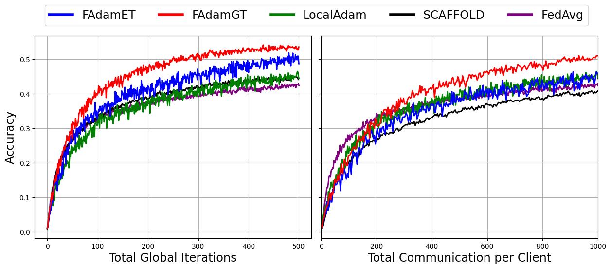
Figure 2: Comparison of achieved accuracy for a given number of global iterations or total communication on CIFAR-100. We can show that our method steadily outperform baselines under different evaluation methods.

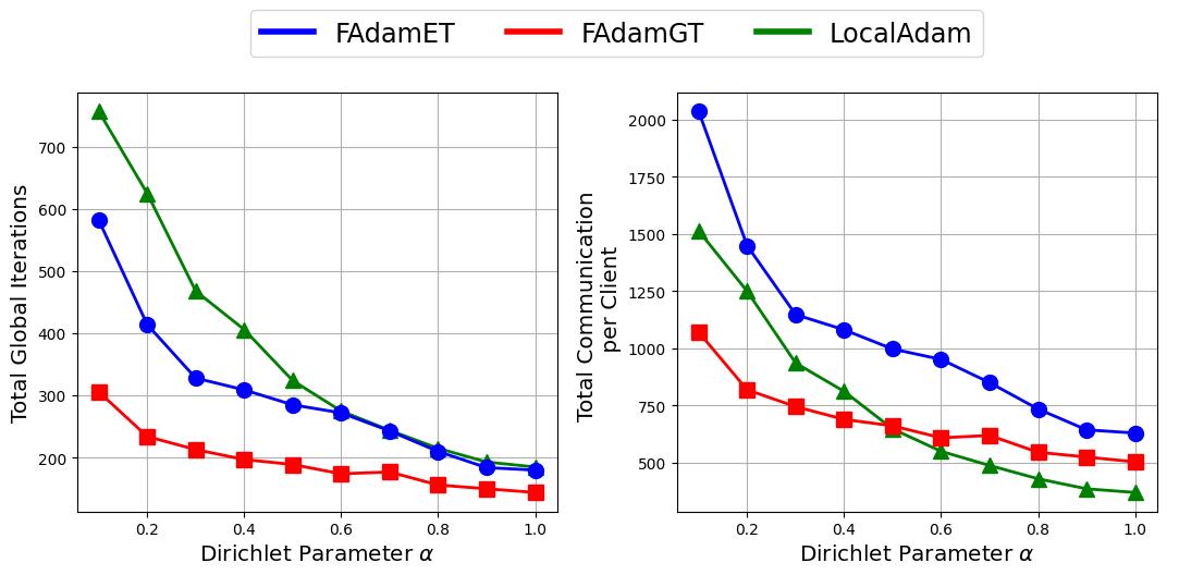
Figure 3: Comparison of the total cost of Adam-based methods under varying Dirichlet parameters on CIFAR-100 to attain $50\%$ accuracy. The results show that, in terms of communication efficiency, the proposed methods are more advantageous in non-i.i.d. settings, where data heterogeneity poses greater challenges.

Figure LABEL:fig:tracking_rate evaluates the performance of our proposed methods under different subset sizes $Y$ used for updating tracking terms. We set the total clients to be $n=100$. In these set of experiments, we increase the client sample size from $S=10$ to $S=50$. This allows a wider range of $Y$ value to compare the difference in terms of communication efficiency. We then compare the communication and computation cost for both algorithms across various $Y$ values ranging from 1 to 50. The results reveal that, for both FAdamET and FAdamGT, the total iterations to achieve certain accuracy under increases slowly as the $Y$ value decreases. This finding demonstrates the possibility to significantly reduce the total number of communications required by the parameter tracking process without compromising training performance. The implication is particularly valuable when communication costs are a major bottleneck.

These findings are further substantiated by the communication per client plots in Figure LABEL:fig:tracking_rate. The plots highlight that the appropriate $Y$ values not only reduces communication overhead but also maintains superior performance compared to all other configurations and baseline methods. This advantage underscores the robustness of parameter tracking in FAdamGT, which effectively balances communication efficiency and convergence. By leveraging a reduced set size $Y$, FAdamGT achieves steady improvements over baselines while preserving its performance.

6.3 Experiments on PEFT tasks using LLMs

In these PEFT tasks, the model weights transmitted between the server and each client account for only 1.9% of the total weights stored locally on the clients. This indicates that the primary bottleneck lies in the computational cost rather than the communication cost. Consequently, we focus on evaluating the performance of each method based on the total number of required global iterations.

Table 2 presents the performance of parameter tracking when integrated into the FedIT framework. In these experiments, the size of the sample set used for model aggregation is equal to the sample set for tracking term aggregation, i.e., $Y=S$. The local epochs between two consecutive global aggregations is set to one, and the target accuracy for each experiment is detailed in Appendix C.

The results demonstrate that while the improvement introduced by ET is less pronounced compared to its impact in CIFAR-100 and TinyImageNet experiments, GT consistently yields significant enhancements over the vanilla version of FedIT. This observation highlights the robustness and adaptability of parameter tracking mechanisms. The substantial improvements achieved by GT emphasize its ability to capture and leverage first-order information effectively during adaptive optimization. This underscores the generalizability of parameter tracking techniques, where a broad family of optimizers can benefit from enhanced convergence rates, showing its potential for advancing large-scale federated learning applications.

Table 2: Required total global iterations for FedIT to attain certain accuracy. The mean and standard deviation is based on four random trials. Though incorporating ET doesn’t bring visible improvement, GT improves the performance of Adam optimizer and results in faster convergence.

Dataset	FedIT- Adam	FedIT- AdamET	FedIT- AdamGT
20NewsGroups	156.8$\pm$7.8	155.0$\pm$7.0	143.3$\pm$4.1
SST-2	47.0$\pm$5.8	48.8$\pm$8.4	30.3$\pm$7.3
QQP	213.0$\pm$53.8	196.3$\pm$5.1	63.0$\pm$4.6
QNLI	117.0$\pm$10.4	99.8$\pm$11.2	55.5$\pm$16.3

7 Conclusion

In this paper, we introduce Parameter Tracking, a general framework for developing FL algorithms that are robust to data heterogeneity. By incorporating parameter tracking into local adaptive optimizers, we propose two novel algorithms: FAdamET and FAdamGT. Through rigorous theoretical analysis, we demonstrate that both algorithms achieve sublinear convergence to a stationary point and reveal the impact of parameter tracking when applied at different stages of the local update process. Comprehensive numerical evaluations confirm that both methods outperform all baselines, delivering superior training performance in heterogeneous data settings. These results pave the way for future advancements in federated optimization algorithms.

Appendix

[sections] [sections]l1

Appendix A Theoretical Analysis for FAdamET (Theorem 1)

We first define the following auxilary definitions that will be helpful throughout the proof.

We define $c^{k}$ as the sum of all moving average coefficients to compute the first order moment $m_{i}^{(t,k)}$:

$$c^{(k,k^{\prime})} =(1-\beta_{1})\beta_{1}^{k-k^{\prime}}$$ (A.0.1)

$$c^{k} =\sum_{k^{\prime}=1}^{k}c^{(k,k^{\prime})}<1$$ (A.0.2)

We first define the unbiased version of $m_{i}^{(t,k)}$ taking expectation on all stochastic gradients $g_{i}^{(t,k)}$. We define $\tilde{m}_{i}^{(t,k)}$ as the following:

$$\tilde{m}_{i}^{(t,k)} \overset{\Delta}{=}\sum_{k^{\prime}=1}^{k}c^{(k,k^{\prime})}\nabla f_{i}(x_{i}^{(t,k)})$$ (A.0.3)

We define an auxilary variable $\alpha_{i}^{t,k}$:

$$\alpha_{i}^{t,k}=\begin{cases}m_{i}^{t-1,k}/(\sqrt{v_{i}^{t-1,k}}+\epsilon),&i\in\mathcal{Y}^{t-1}\\ \alpha_{i}^{t-1,k},&i\notin\mathcal{Y}^{t-1}\end{cases}$$ (A.0.4)

We define the tracking variable drift term as:

$$\Gamma^{(t)}=\frac{1}{nK}\sum_{i=1}^{n}\sum_{k=1}^{K}\mathbb{E}\left\|\alpha_{i}^{t,k}-\nabla f_{i}(x^{(t)})\right\|^{2}$$ (A.0.5)

We define the local update deviation term as:

$$\mathcal{E}^{(t)}=\frac{1}{n}\sum_{i=1}^{n}\sum_{k=1}^{K}\mathbb{E}\|\tilde{m}_{i}^{(t,k)}-c^{k}\nabla f_{i}(x^{(t)})\|^{2}$$ (A.0.6)

Proof.

Given global iteration $t$, the update of the model at the server can be written as:

$$x^{(t+1)} =x^{(t)}+\eta_{g}\frac{1}{S}\sum_{i\in\mathcal{S}^{(t)}}(x_{i}^{(t,K+1)}-x^{(t)})$$ (A.0.7)

$$=x^{(t)}-\eta_{g}\eta_{l}\frac{1}{S}\sum_{i\in\mathcal{S}^{(t)}}\sum_{k=1}^{K}\frac{m_{i}^{(t,k)}}{\sqrt{\hat{v}_{i}^{(t,k)}}+\epsilon}$$ (A.0.8)

By injecting Assumption 1, we can get the following inequality:

$$\mathbb{E}f(x^{(t+1)})\leq \mathbb{E}f(x^{(t)})-\underbrace{\eta_{g}\eta_{l}\mathbb{E}\left\langle\nabla f(x^{(t)}),\frac{1}{|\mathcal{S}^{(t)}|}\sum_{i\in\mathcal{S}^{(t)}}\sum_{k=1}^{K}\frac{m_{i}^{(t,k)}}{\sqrt{\hat{v}_{i}^{(t,k)}}+\epsilon}\right\rangle}_{\text{Term I}}$$ (A.0.9)

$$+\underbrace{\eta_{g}^{2}\eta_{l}^{2}\frac{L}{2}\mathbb{E}\left\|\frac{1}{|\mathcal{S}^{(t)}|}\sum_{i\in\mathcal{S}^{(t)}}\sum_{k=1}^{K}\frac{m_{i}^{(t,k)}}{\sqrt{\hat{v}_{i}^{(t,k)}}+\epsilon}\right\|^{2}}_{\text{Term II}}$$ (A.0.10)

For term I, we first define the average of all square root second moment:

$$\bar{v}^{(t)}=\frac{1}{n}\sum_{i=1}^{n}\sqrt{v_{i}^{(t)}}$$ (A.0.11)

Then we can upper bound it by Assumption 1:

$$-\eta_{g}\eta_{l}\mathbb{E}\left\langle\nabla f(x^{(t)}),\frac{1}{S}\sum_{i\in\mathcal{S}^{(t)}}\sum_{k=1}^{K}\frac{m_{i}^{(t,k)}}{\sqrt{\hat{v}_{i}^{(t,k)}}+\epsilon}\right\rangle$$ (A.0.12)

$$-\eta_{g}\eta_{l}\mathbb{E}\left\langle\nabla f(x^{(t)}),\frac{1}{S}\sum_{i\in\mathcal{S}^{(t)}}\sum_{k=1}^{K}\frac{\tilde{m}_{i}^{(t,k)}}{\sqrt{\hat{v}_{i}^{(t,k)}}+\epsilon}\right\rangle$$ (A.0.13)

$$=-\eta_{g}\eta_{l}\mathbb{E}\left\langle\nabla f(x^{(t)}),\frac{1}{n}\sum_{i=1}^{n}\sum_{k=1}^{K}\left(\frac{\tilde{m}_{i}^{(t,k)}}{\sqrt{\hat{v}_{i}^{(t,k)}}+\epsilon}-\frac{\tilde{m}_{i}^{(t,k)}}{{\bar{v}^{(t)}}+\epsilon}+\frac{\tilde{m}_{i}^{(t,k)}}{{\bar{v}^{(t)}}+\epsilon}-\frac{c^{k}\nabla f_{i}(x^{(t)})}{{\bar{v}^{(t)}}+\epsilon}+\frac{c^{k}\nabla f_{i}(x^{(t)})}{{\bar{v}^{(t)}}+\epsilon}\right)\right\rangle$$ (A.0.14)

$$\overset{(a)}{\leq}-\eta_{g}\eta_{l}K\frac{(1-\beta_{1})\beta_{1}}{G+\epsilon}\mathbb{E}\|\nabla f(x^{(t)}\|^{2}$$ (A.0.15)

$$-\eta_{g}\eta_{l}K\mathbb{E}\left\langle\nabla f(x^{(t+1)}),\frac{1}{nK}\sum_{i=1}^{n}\sum_{k=1}^{K}\left(\frac{\tilde{m}_{i}^{(t,k)}}{\sqrt{\hat{v}_{i}^{(t,k)}}+\epsilon}-\frac{\tilde{m}_{i}^{(t,k)}}{{\bar{v}^{(t)}}+\epsilon}+\frac{\tilde{m}_{i}^{(t,k)}}{{\bar{v}^{(t)}}+\epsilon}-\frac{c^{k}\nabla f_{i}(x^{(t)})}{{\bar{v}^{(t)}}+\epsilon}\right)\right\rangle$$ (A.0.16)

$$\leq-\frac{\eta_{g}\eta_{l}K}{2}\frac{(1-\beta_{1})\beta_{1}}{G+\epsilon}\mathbb{E}\|\nabla f(x^{(t)}\|^{2}+\eta_{g}\eta_{l}\frac{G+\epsilon}{(1-\beta_{1})\beta_{1}\epsilon^{2}}\frac{1}{n}\sum_{i=1}^{n}\sum_{k=1}^{K}\mathbb{E}\|\tilde{m}_{i}^{(t,k)}-c^{k}\nabla f_{i}(x^{(t)})\|^{2}$$ (A.0.17)

$$+\eta_{g}\eta_{l}K\frac{G+\epsilon}{(1-\beta_{1})\beta_{1}}\mathbb{E}\|\frac{1}{nK}\sum_{i=1}^{n}\sum_{k=1}^{K}\frac{\tilde{m}_{i}^{(t,k)}}{\sqrt{\hat{v}_{i}^{(t,k)}}+\epsilon}-\frac{\tilde{m}_{i}^{(t,k)}}{{\bar{v}^{(t)}}+\epsilon}\|^{2}$$ (A.0.18)

$$\leq-\frac{\eta_{g}\eta_{l}K}{2}\frac{(1-\beta_{1})\beta_{1}}{G+\epsilon}\mathbb{E}\|\nabla f(x^{(t)}\|^{2}+\eta_{g}\eta_{l}\frac{G+\epsilon}{(1-\beta_{1})\beta_{1}\epsilon^{2}}\frac{1}{n}\sum_{i=1}^{n}\sum_{k=1}^{K}\mathbb{E}\|\tilde{m}_{i}^{(t,k)}-c^{k}\nabla f_{i}(x^{(t)})\|^{2}$$ (A.0.19)

$$+\eta_{g}\eta_{l}K\frac{G^{2}(G+\epsilon)}{(1-\beta_{1})\beta_{1}}\mathbb{E}\|\frac{1}{nK}\sum_{i=1}^{n}\sum_{k=1}^{K}\frac{\sqrt{\hat{v}_{i}^{(t,k)}}-\bar{v}^{(t)}}{(\sqrt{\hat{v}_{i}^{(t,k)}}+\epsilon)(\bar{v}^{(t)}+\epsilon)}\|^{2}$$ (A.0.20)

$$\overset{(b)}{\leq}-\frac{\eta_{g}\eta_{l}K}{2}\frac{(1-\beta_{1})\beta_{1}}{G+\epsilon}\mathbb{E}\|\nabla f(x^{(t)}\|^{2}+\eta_{g}\eta_{l}\frac{G+\epsilon}{(1-\beta_{1})\beta_{1}\epsilon^{2}}\frac{1}{n}\sum_{i=1}^{n}\sum_{k=1}^{K}\mathbb{E}\|\tilde{m}_{i}^{(t,k)}-c^{k}\nabla f_{i}(x^{(t)})\|^{2}$$ (A.0.21)

$$+\eta_{g}\eta_{l}K\frac{G^{2}(G+\epsilon)}{(1-\beta_{1})\beta_{1}\epsilon^{2}}\mathbb{E}\|\bar{v}^{(t+1)}-\bar{v}^{(t)}\|^{2}$$ (A.0.22)

Where (a) the fact that $(1-\beta_{1})\beta_{1}\leq c^{k}\leq\beta_{1}$, and (b) uses the fact that $\hat{v}_{i}^{(t,1)}\leq\hat{v}_{i}^{(t,2)}\leq\ldots\leq\hat{v}_{i}^{(t,K+1)}$.

For term II, we can bound it as:

$$\frac{\eta_{g}^{2}\eta_{l}^{2}L}{2}\mathbb{E}\left\|\frac{1}{|\mathcal{S}^{(t)}|}\sum_{i\in\mathcal{S}^{(t)}}\sum_{k=1}^{K}\frac{m_{i}^{(t,k)}}{\sqrt{\hat{v}_{i}^{(t,k)}}+\epsilon}\right\|^{2}=\eta_{g}^{2}\eta_{l}^{2}L\mathbb{E}\left\|\frac{1}{n}\sum_{i=1}^{n}\sum_{k=1}^{K}\frac{\tilde{m}_{i}^{(t,k)}}{\sqrt{\hat{v}_{i}^{(t,k)}}+\epsilon}\right\|^{2}+\eta_{g}^{2}\eta_{l}^{2}KL\sigma^{2}$$ (A.0.23)

$$=\eta_{g}^{2}\eta_{l}^{2}L\mathbb{E}\left\|\frac{1}{n}\sum_{i=1}^{n}\sum_{k=1}^{K}\frac{\tilde{m}_{i}^{(t,k)}}{\sqrt{\hat{v}_{i}^{(t,k)}}+\epsilon}-\nabla f_{i}(x^{(t)})+\nabla f_{i}(x^{(t)})\right\|^{2}+\eta_{g}^{2}\eta_{l}^{2}KL\sigma^{2}$$ (A.0.24)

$$\leq 2\eta_{g}^{2}\eta_{l}^{2}K^{2}L\mathbb{E}\|\nabla f(x^{(t)}\|^{2}+2\eta_{g}^{2}\eta_{l}^{2}L\frac{K}{n}\sum_{i=1}^{n}\sum_{k=1}^{K}\|\frac{\tilde{m}_{i}^{(t,k)}}{\sqrt{\hat{v}_{i}^{(t,k)}}+\epsilon}-\frac{c^{k}\nabla f_{i}(x^{(t)})}{\sqrt{\hat{v}_{i}^{(t,k)}}+\epsilon}+\frac{c^{k}\nabla f_{i}(x^{(t)})}{\sqrt{\hat{v}_{i}^{(t,k)}}+\epsilon}-\nabla f_{i}(x^{(t)})\|^{2}$$ (A.0.25)

$$+\eta_{g}^{2}\eta_{l}^{2}KL\sigma^{2}$$ (A.0.26)

$$\leq 2\eta_{g}^{2}\eta_{l}^{2}K^{2}L\mathbb{E}\|\nabla f(x^{(t)}\|^{2}+\frac{4\eta_{g}^{2}\eta_{l}^{2}KL}{\epsilon^{2}}\frac{1}{n}\sum_{i=1}^{n}\sum_{k=1}^{K}\|\tilde{m}_{i}^{(t,k)}-c^{k}\nabla f_{i}(x^{(t)})\|^{2}+\frac{4\eta_{g}^{2}\eta_{l}^{2}(1-\epsilon)^{2}}{\epsilon^{2}}K^{2}LG^{2}$$ (A.0.27)

$$+\eta_{g}^{2}\eta_{l}^{2}KL\sigma^{2}$$ (A.0.28)

If we choose $\eta_{g}\eta_{l}\leq\min(\frac{(1-\beta_{1})\beta_{1}}{8KL(G+\epsilon)},\frac{1}{4KL})$, we can combine Term I and II and get:

$$\mathbb{E}f(x^{(t+1)})\leq \mathbb{E}f(x^{(t)})-\frac{\eta_{g}\eta_{l}K}{4}\frac{(1-\beta_{1})\beta_{1}}{G+\epsilon}\mathbb{E}\|\nabla f(x^{(t)}\|^{2}+\frac{\eta_{g}\eta_{l}}{\epsilon^{2}}\left(\frac{G+\epsilon}{(1-\beta_{1})\beta_{1}}+\frac{1}{2}\right)\mathcal{E}^{(t)}$$ (A.0.29)

$$+\eta_{g}\eta_{l}K\frac{G^{2}(G+\epsilon)}{(1-\beta_{1})\beta_{1}\epsilon^{2}}\mathbb{E}\|\bar{v}^{(t+1)}-\bar{v}^{(t)}\|^{2}+\frac{2\eta_{g}^{2}\eta_{l}^{2}(1-\epsilon)^{2}}{\epsilon^{2}}K^{2}LG^{2}+\eta_{g}^{2}\eta_{l}^{2}KL\sigma^{2}$$ (A.0.30)

By using Lemma A.0.1, we can formulate the following:

$$\mathbb{E}f(x^{(t+1)})\leq \mathbb{E}f(x^{(t)})\left(-\frac{\eta_{g}\eta_{l}K}{4}\frac{(1-\beta_{1})\beta_{1}}{G+\epsilon}+\frac{\eta_{g}\eta_{l}}{\epsilon^{2}}\left(\frac{G+\epsilon}{(1-\beta_{1})\beta_{1}}+\frac{1}{2}\right)48\eta_{l}^{2}K^{3}L^{2}\right)\mathbb{E}\|\nabla f(x^{(t)}\|^{2}$$ (A.0.31)

$$+\frac{\eta_{g}\eta_{l}}{\epsilon^{2}}\left(\frac{G+\epsilon}{(1-\beta_{1})\beta_{1}}+\frac{1}{2}\right)96K^{3}L^{2}\eta_{l}^{2}\Gamma^{(t)}$$ (A.0.32)

$$+\eta_{g}\eta_{l}K\frac{G^{2}(G+\epsilon)}{(1-\beta_{1})\beta_{1}\epsilon^{2}}\mathbb{E}\|\bar{v}^{(t+1)}-\bar{v}^{(t)}\|^{2}$$ (A.0.33)

$$+\frac{2\eta_{g}^{2}\eta_{l}^{2}(1-\epsilon)^{2}}{\epsilon^{2}}K^{2}LG^{2}+\frac{\eta_{g}\eta_{l}}{\epsilon^{2}}\left(\frac{G+\epsilon}{(1-\beta_{1})\beta_{1}}+\frac{1}{2}\right)144K^{3}L^{2}\eta_{l}^{2}\left(\frac{G^{2}(1+\epsilon)+\sigma^{2}}{\epsilon}\right)$$ (A.0.34)

$$+\eta_{g}^{2}\eta_{l}^{2}KL\sigma^{2}$$ (A.0.35)

By choosing the local step size as $\eta_{l}\leq\frac{\sqrt{G+\epsilon+(1-\beta_{1})\beta_{1}}\sqrt{G+\epsilon}}{12\sqrt{2}(1-\beta_{1})\beta_{1}KL}$, we can get:

$$\frac{\eta_{g}\eta_{l}K}{12}\frac{(1-\beta_{1})\beta_{1}}{G+\epsilon}\mathbb{E}\|\nabla f(x^{(t)}\|^{2} \leq\mathbb{E}f(x^{(t)})-\mathbb{E}f(x^{(t+1)})$$ (A.0.36)

$$+\frac{\eta_{g}\eta_{l}}{\epsilon^{2}}\left(\frac{G+\epsilon}{(1-\beta_{1})\beta_{1}}+\frac{1}{2}\right)96K^{3}L^{2}\eta_{l}^{2}\Gamma^{(t)}$$ (A.0.37)

$$+\eta_{g}\eta_{l}K\frac{G^{2}(G+\epsilon)}{(1-\beta_{1})\beta_{1}\epsilon^{2}}\mathbb{E}\|\bar{v}^{(t+1)}-\bar{v}^{(t)}\|^{2}$$ (A.0.38)

$$+\frac{2\eta_{g}^{2}\eta_{l}^{2}(1-\epsilon)^{2}}{\epsilon^{2}}K^{2}LG^{2}+\frac{\eta_{g}\eta_{l}}{\epsilon^{2}}\left(\frac{G+\epsilon}{(1-\beta_{1})\beta_{1}}+\frac{1}{2}\right)144K^{3}L^{2}\eta_{l}^{2}\left(\frac{G^{2}(1+\epsilon)+\sigma^{2}}{\epsilon}\right)$$ (A.0.39)

$$+\eta_{g}^{2}\eta_{l}^{2}KL\sigma^{2}$$ (A.0.40)

By moving constants across the inequality and taking average over all iterations, we can get:

$$\frac{1}{T}\sum_{t=1}^{T}\mathbb{E}\|\nabla f(x^{(t)}\|^{2} \leq\frac{12(G+\epsilon)(\mathbb{E}f(x^{(1)})-\mathbb{E}f(x^{(T+1)}))}{\eta_{g}\eta_{l}K(1-\beta_{1})\beta_{1}T}$$ (A.0.41)

$$+\frac{12}{K\epsilon^{2}}\left(\frac{G+\epsilon}{(1-\beta_{1})\beta_{1}}+\frac{1}{2}\right)^{2}96K^{3}L^{2}\eta_{l}^{2}\sum_{t=1}^{T}\Gamma^{(t)}$$ (A.0.42)

$$+\frac{12G^{2}(G+\epsilon)^{2}}{(1-\beta_{1})^{2}\beta_{1}^{2}\epsilon^{2}T}\mathbb{E}\|\bar{v}^{(T+1)}-\bar{v}^{(1)}\|^{2}$$ (A.0.43)

$$+\frac{24\eta_{g}\eta_{l}(1-\epsilon)^{2}KLG^{2}(G+\epsilon)}{(1-\beta_{1})\beta_{1}\epsilon^{2}}$$ (A.0.44)

$$+\frac{12}{\epsilon^{2}}\left(\frac{G+\epsilon}{(1-\beta_{1})\beta_{1}}+\frac{1}{2}\right)^{2}144K^{2}L^{2}\eta_{l}^{2}\left(\frac{G^{2}(1+\epsilon)+\sigma^{2}}{\epsilon}\right)$$ (A.0.45)

$$+\frac{12\eta_{g}\eta_{l}L(G+\epsilon)}{(1-\beta_{1})\beta_{1}}\sigma^{2}$$ (A.0.46)

By using Lemma A.0.2, we can bound $\sum_{t=1}^{T}\Gamma^{(t)}$ with:

$$\sum_{t=1}^{T}\Gamma^{(t)} \leq\sum_{t=1}^{T}(1-\frac{Y}{2n})^{T-t}\Gamma^{(1)}+T^{2}\frac{Y}{n}\left(\frac{G^{2}(1+\epsilon)+\sigma^{2}}{\epsilon}+6n^{2}G^{2}\right)$$ (A.0.47)

$$=T^{2}\frac{Y}{n}\left(\frac{G^{2}(1+\epsilon)+\sigma^{2}}{\epsilon}+6n^{2}G^{2}\right)$$ (A.0.48)

Finally, by bounding $\eta_{l}\leq\frac{1}{12T^{3/2}L}$, $\eta_{g}\eta_{l}\leq\frac{1}{12TL}$, and a specific step size

$$\eta_{g}\eta_{l}=\min(\frac{(1-\beta_{1})\beta_{1}}{8KL(G+\epsilon)},\frac{1}{4KL},\frac{1}{12TL},\sqrt{\frac{S}{T}})$$ (A.0.49)

we can get the convergence rate:

$$\frac{1}{T}\sum_{t=1}^{T}\mathbb{E}\|\nabla f(x^{(t)}\|^{2} \leq\frac{12(G+\epsilon)(\mathbb{E}f(x^{(1)})-\mathbb{E}f(x^{(T+1)}))}{K(1-\beta_{1})\beta_{1}\sqrt{ST}}$$ (A.0.50)

$$+\left(\frac{G+\epsilon}{(1-\beta_{1})\beta_{1}}+\frac{1}{2}\right)^{2}\left(\frac{G^{2}(1+\epsilon)+\sigma^{2}}{\epsilon}+6n^{2}G^{2}\right)\frac{12YK^{2}}{\epsilon^{2}nT}$$ (A.0.51)

$$+\frac{24G^{4}(G+\epsilon)^{2}}{(1-\beta_{1})^{2}\beta_{1}^{2}\epsilon^{2}T}$$ (A.0.52)

$$+\frac{2(1-\epsilon)^{2}KG^{2}(G+\epsilon)}{(1-\beta_{1})\beta_{1}\epsilon^{2}T}$$ (A.0.53)

$$+\left(\frac{G+\epsilon}{(1-\beta_{1})\beta_{1}}+\frac{1}{2}\right)^{2}\left(\frac{G^{2}(1+\epsilon)+\sigma^{2}}{\epsilon}\right)\frac{12K^{2}}{\epsilon^{2}T^{3}}$$ (A.0.54)

$$+\frac{12(G+\epsilon)}{(1-\beta_{1})\beta_{1}T}\sigma^{2}$$ (A.0.55)

$$=\mathcal{O}\left(\frac{\mathbb{E}f(x^{(1)})-f^{*}}{K\sqrt{ST}}+\frac{1}{T}+\frac{K}{T}+\frac{YK^{2}}{T}+\frac{K^{2}}{T^{3}}\right)$$ (A.0.56)

∎

Lemma A.0.1.

Under Assumption 1, the local devation term $\mathcal{E}^{(t)}=\frac{1}{n}\sum_{i=1}^{n}\sum_{k=1}^{K}\mathbb{E}\|\tilde{m}_{i}^{(t,k)}-c^{k}\nabla f_{i}(x^{(t)})\|^{2}$ can be bounded as the following:

$$\mathcal{E}^{(t)}\leq 48K^{3}L^{2}\eta_{l}^{2}\|\nabla f(x^{(t)})\|^{2}+96K^{3}L^{2}\eta_{l}^{2}\Gamma^{(t)}+144K^{3}L^{2}\eta_{l}^{2}\left(\frac{G^{2}(1+\epsilon)+\sigma^{2}}{\epsilon}\right)$$ (A.0.57)

Proof.

$$\frac{1}{n}\sum_{i=1}^{n}\sum_{k=1}^{K}\mathbb{E}\|\tilde{m}_{i}^{(t,k)}-c^{k}\nabla f_{i}(x^{(t)})\|^{2}$$ (A.0.58)

$$=\frac{1}{n}\sum_{i=1}^{n}\sum_{k=1}^{K}\mathbb{E}\|\sum_{k^{\prime}=1}^{k}c^{(k,k^{\prime})}\left(\nabla f_{i}(x_{i}^{(t,k^{\prime})})-\nabla f_{i}(x^{(t)})\right)\|^{2}$$ (A.0.59)

$$\leq\frac{L^{2}}{n}\sum_{i=1}^{n}\sum_{k=1}^{K}\sum_{k^{\prime}=1}^{k}c^{(k,k^{\prime})}\mathbb{E}\|x_{i}^{(t,k^{\prime})}-x^{(t)}\|^{2}$$ (A.0.60)

We can simplify the formulation by first unfolding each local step $x_{i}^{(t,k^{\prime})}$:

$$\frac{1}{n}\sum_{i=1}^{n}\mathbb{E}\|x_{i}^{(t,k^{\prime})}-x^{(t)}\|^{2}$$ (A.0.61)

$$\leq(1+\frac{1}{K-1})\frac{1}{n}\sum_{i=1}^{n}\mathbb{E}\|x_{i}^{(t,k^{\prime}-1)}-x^{(t)}\|^{2}$$ (A.0.62)

$$+K\frac{1}{n}\sum_{i=1}^{n}\mathbb{E}\left\|\eta_{l}\left(\frac{m_{i}^{(t,k^{\prime}-1)}}{\sqrt{\hat{v}_{i}^{(t,k^{\prime}-1)}}+\epsilon}-\nabla f_{i}(x^{(t)})+y^{(t)}-y_{i}^{(t)}+\nabla f_{i}(x^{(t)})-\nabla f(x^{(t)})+\nabla f(x^{(t)})\right)\right\|^{2}$$ (A.0.63)

$$\leq(1+\frac{1}{K-1})\frac{1}{n}\sum_{i=1}^{n}\mathbb{E}\|x_{i}^{(t,k^{\prime}-1)}-x^{(t)}\|^{2}+3K\eta_{l}^{2}\mathbb{E}\|\nabla f(x^{(t)})\|^{2}+3K\eta_{l}^{2}\Gamma^{(t)}+12K\eta_{l}^{2}\left(\frac{G^{2}(1+\epsilon)+\sigma^{2}}{\epsilon}\right)$$ (A.0.64)

$$\leq\sum_{r=1}^{k^{\prime}}(1+\frac{1}{K-1})^{r}\left(4K\eta_{l}^{2}\mathbb{E}\|\nabla f(x^{(t)})\|^{2}+8K\eta_{l}^{2}\frac{1}{nK}\sum_{i=1}^{n}\sum_{k^{\prime\prime}=1}^{K}\|\alpha_{i}^{t,k^{\prime\prime}}-\nabla f_{i}(x^{(t)})\|^{2}\right)$$ (A.0.65)

$$+\sum_{r=1}^{k^{\prime}}(1+\frac{1}{K-1})^{r}12K\eta_{l}^{2}\left(\frac{G^{2}(1+\epsilon)+\sigma^{2}}{\epsilon}\right)$$ (A.0.66)

Using the fact that $(1+\frac{1}{K-1})^{r}\leq 2e\leq 6$, we can get that:

$$\frac{1}{n}\sum_{i=1}^{n}\sum_{k=1}^{K}\mathbb{E}\|m_{i}^{(t,k)}-c^{k}\nabla f_{i}(x^{(t)})\|^{2}\leq 48K^{3}L^{2}\eta_{l}^{2}\|\nabla f(x^{(t)})\|^{2}+96K^{3}L^{2}\eta_{l}^{2}\Gamma^{(t)}+144K^{3}L^{2}\eta_{l}^{2}\left(\frac{G^{2}(1+\epsilon)+\sigma^{2}}{\epsilon}\right)$$ (A.0.67)

∎

Lemma A.0.2.

Under Assumption 2, the tracking variable drift term $\Gamma^{(t)}=\frac{1}{nK}\sum_{i=1}^{n}\sum_{k=1}^{K}\mathbb{E}\left\|\alpha_{i}^{t,k}-\nabla f_{i}(x^{(t)})\right\|^{2}$ can be bounded as:

$$\Gamma^{(t)}\leq(1-\frac{Y}{n})\Gamma^{(t-1)}+\frac{Y}{n}\left(\frac{G^{2}(1+\epsilon)+\sigma^{2}}{\epsilon}\right)$$ (A.0.68)

Proof.

By using the definition of $\alpha_{i}^{t,k}$, we can get the following relation:

$$\Gamma^{(t)} =\frac{1}{nK}\sum_{i=1}^{n}\sum_{k=1}^{K}\mathbb{E}\left\|\alpha_{i}^{t,k}-\nabla f_{i}(x^{(t)})\right\|^{2}$$ (A.0.69)

$$\leq(1-\frac{Y}{n})(1+\frac{Y}{2n})\frac{1}{nK}\sum_{i=1}^{n}\sum_{k=1}^{K}\mathbb{E}\left\|\alpha_{i}^{t-1,k}-\nabla f_{i}(x^{(t-1)})\right\|^{2}+2(1+\frac{2n}{Y})G^{2}$$ (A.0.70)

$$+\frac{Y}{n}\frac{1}{nK}\sum_{i=1}^{n}\sum_{k=1}^{K}\mathbb{E}\left\|\frac{m_{i}^{t-1,k}}{\sqrt{v_{i}^{t-1,k}}+\epsilon}-\nabla f_{i}(x^{(t)})\right\|^{2}$$ (A.0.71)

$$\leq(1-\frac{Y}{2n})\Gamma^{(t-1)}+\frac{Y}{n}\left(\frac{G^{2}(1+\epsilon)+\sigma^{2}}{\epsilon}+6n^{2}G^{2}\right)$$ (A.0.72)

∎

Appendix B Theoretical Analysis for FAdamGT (Theorem 1)

We first define the expected first order moment $\tilde{m}_{i}^{(t,k)}$ as the following:

$$\tilde{m}_{i}^{(t,k)} \overset{\Delta}{=}\sum_{k^{\prime}=1}^{k}c^{(k,k^{\prime})}\left(\nabla f_{i}(x_{i}^{(t,k)})-\nabla f_{i}(\gamma_{i}^{(t,k)})+\frac{1}{n}\sum_{i=1}^{n}\nabla f_{i}(\gamma_{i}^{(t,k)})\right)$$ (B.0.1)

Where $\gamma_{i}^{(t,k)}$ is an auxilary variable that tracks the GT terms:

$$\gamma_{i}^{(t,k)}=\begin{cases}x_{i}^{(t-1,k)}\quad i\in\mathcal{Y}^{t-1}\\ \gamma_{i}^{(t-1,k)}\quad i\notin\mathcal{Y}^{t-1}\end{cases}$$ (B.0.2)

We further define the local deviation term $\Xi^{(t)}$ as:

$$\Xi^{(t)}=\frac{1}{n}\sum_{i=1}^{n}\sum_{k=1}^{K}\mathbb{E}\|\sum_{k^{\prime}=1}^{k}c^{(k,k^{\prime})}\nabla f_{i}(x_{i}^{(t,k^{\prime})})-c^{k}\nabla f_{i}(x^{(t)})\|^{2}$$ (B.0.3)

Proof.

Given global iteration $t$, the update of the model at the server can be written as:

$$x^{(t+1)} =x^{(t)}+\eta_{g}\frac{1}{S}\sum_{i\in\mathcal{S}^{(t)}}(x_{i}^{(t,K+1)}-x^{(t)})$$ (B.0.4)

$$=x^{(t)}-\eta_{g}\eta_{l}\frac{1}{S}\sum_{i\in\mathcal{S}^{(t)}}\sum_{k=1}^{K}\frac{m_{i}^{(t,k)}}{\sqrt{\hat{v}_{i}^{(t,k)}}+\epsilon}$$ (B.0.5)

By injecting Assumption 1, we can get the following inequality:

$$\mathbb{E}f(x^{(t+1)})\leq \mathbb{E}f(x^{(t)})-\underbrace{\eta_{g}\eta_{l}\mathbb{E}\left\langle\nabla f(x^{(t)}),\frac{1}{S}\sum_{i\in\mathcal{S}^{(t)}}\sum_{k=1}^{K}\frac{m_{i}^{(t,k)}}{\sqrt{\hat{v}_{i}^{(t,k)}}+\epsilon}\right\rangle}_{\text{Term I}}$$ (B.0.6)

$$+\underbrace{\eta_{g}^{2}\eta_{l}^{2}\frac{L}{2}\mathbb{E}\left\|\frac{1}{S}\sum_{i\in\mathcal{S}^{(t)}}\sum_{k=1}^{K}\frac{m_{i}^{(t,k)}}{\sqrt{\hat{v}_{i}^{(t,k)}}+\epsilon}\right\|^{2}}_{\text{Term II}}$$ (B.0.7)

For term I, we first define the average of all square root second moment:

$$\bar{v}^{(t)}=\frac{1}{n}\sum_{i=1}^{n}\sqrt{v_{i}^{(t)}}$$ (B.0.8)

Term I can be upper bounded as:

$$-\eta_{g}\eta_{l}\mathbb{E}\left\langle\nabla f(x^{(t)}),\frac{1}{S}\sum_{i\in\mathcal{S}^{(t)}}\sum_{k=1}^{K}\frac{m_{i}^{(t,k)}}{\sqrt{\hat{v}_{i}^{(t,k)}}+\epsilon}\right\rangle$$ (B.0.9)

$$=-\eta_{g}\eta_{l}\mathbb{E}\left\langle\nabla f(x^{(t)}),\frac{1}{S}\sum_{i\in\mathcal{S}^{(t)}}\sum_{k=1}^{K}\frac{\tilde{m}_{i}^{(t,k)}}{\sqrt{\hat{v}_{i}^{(t,k)}}+\epsilon}\right\rangle$$ (B.0.10)

$$=-\eta_{g}\eta_{l}\mathbb{E}\left\langle\nabla f(x^{(t)}),\frac{1}{n}\sum_{i=1}^{n}\sum_{k=1}^{K}\frac{\sum_{k^{\prime}=1}^{k}c^{(k,k^{\prime})}\left(\nabla f_{i}(x_{i}^{(t,k^{\prime})})+\frac{1}{K}\sum_{k^{\prime\prime}=1}^{K}\left(\frac{1}{n}\sum_{i^{\prime}=1}^{n}\nabla f_{i}^{\prime}(\gamma_{i}^{\prime(t,k^{\prime\prime})})-\nabla f_{i}(\gamma_{i}^{(t,k^{\prime\prime})})\right)\right)}{\sqrt{\hat{v}_{i}^{(t,k)}}+\epsilon}\right\rangle$$ (B.0.11)

Using the fact that $\sum_{i=1}^{n}\left(\nabla f_{i}(\gamma_{i}^{(t,k)})-\frac{1}{n}\sum_{i^{\prime}=1}^{n}\nabla f_{i}^{\prime}(\gamma_{i}^{\prime(t,k)})\right)=0$, we can show that:

$$-\eta_{g}\eta_{l}\mathbb{E}\left\langle\nabla f(x^{(t)}),\frac{1}{S}\sum_{i\in\mathcal{S}^{(t)}}\sum_{k=1}^{K}\frac{m_{i}^{(t,k)}}{\sqrt{\hat{v}_{i}^{(t,k)}}+\epsilon}\right\rangle$$ (B.0.13)

$$=-\eta_{g}\eta_{l}\mathbb{E}\left\langle\nabla f(x^{(t)}),\frac{1}{n}\sum_{i=1}^{n}\sum_{k=1}^{K}\left(\frac{\sum_{k^{\prime}=1}^{k}c^{(k,k^{\prime})}\nabla f_{i}(x_{i}^{(t,k^{\prime})})}{\sqrt{\hat{v}_{i}^{(t,k)}}+\epsilon}-\frac{\sum_{k^{\prime}=1}^{k}c^{(k,k^{\prime})}\nabla f_{i}(x_{i}^{(t,k^{\prime})})}{{\bar{v}^{(t)}}+\epsilon}\right)\right\rangle$$ (B.0.14)

$$-\eta_{g}\eta_{l}\mathbb{E}\left\langle\nabla f(x^{(t)}),\frac{1}{n}\sum_{i=1}^{n}\sum_{k=1}^{K}\left(\frac{\sum_{k^{\prime}=1}^{k}c^{(k,k^{\prime})}\nabla f_{i}(x_{i}^{(t,k^{\prime})})}{{\bar{v}^{(t)}}+\epsilon}-\frac{c^{k}\nabla f_{i}(x^{(t)})}{{\bar{v}^{(t)}}+\epsilon}+\frac{c^{k}\nabla f_{i}(x^{(t)})}{{\bar{v}^{(t)}}+\epsilon}\right)\right\rangle$$ (B.0.15)

$$\leq-\eta_{g}\eta_{l}K\frac{(1-\beta_{1})\beta_{1}}{G+\epsilon}\mathbb{E}\|\nabla f(x^{(t)}\|^{2}$$ (B.0.16)

$$-\eta_{g}\eta_{l}\mathbb{E}\left\langle\nabla f(x^{(t)}),\frac{1}{n}\sum_{i=1}^{n}\sum_{k=1}^{K}\left(\frac{\sum_{k^{\prime}=1}^{k}c^{(k,k^{\prime})}\nabla f_{i}(x_{i}^{(t,k^{\prime})})}{\sqrt{\hat{v}_{i}^{(t,k)}}+\epsilon}-\frac{\sum_{k^{\prime}=1}^{k}c^{(k,k^{\prime})}\nabla f_{i}(x_{i}^{(t,k^{\prime})})}{{\bar{v}^{(t)}}+\epsilon}\right)\right\rangle$$ (B.0.17)

$$-\eta_{g}\eta_{l}\mathbb{E}\left\langle\nabla f(x^{(t)}),\frac{1}{n}\sum_{i=1}^{n}\sum_{k=1}^{K}\left(\frac{\sum_{k^{\prime}=1}^{k}c^{(k,k^{\prime})}\nabla f_{i}(x_{i}^{(t,k^{\prime})})}{{\bar{v}^{(t)}}+\epsilon}-\frac{c^{k}\nabla f_{i}(x^{(t)})}{{\bar{v}^{(t)}}+\epsilon}\right)\right\rangle$$ (B.0.18)

$$\leq-\frac{\eta_{g}\eta_{l}K}{2}\frac{(1-\beta_{1})\beta_{1}}{G+\epsilon}\mathbb{E}\|\nabla f(x^{(t)}\|^{2}+\eta_{g}\eta_{l}\frac{G+\epsilon}{(1-\beta_{1})\beta_{1}\epsilon^{2}}\frac{1}{n}\sum_{i=1}^{n}\sum_{k=1}^{K}\mathbb{E}\|\sum_{k^{\prime}=1}^{k}c^{(k,k^{\prime})}\nabla f_{i}(x_{i}^{(t,k^{\prime})})-c^{k}\nabla f_{i}(x^{(t)})\|^{2}$$ (B.0.19)

$$+\eta_{g}\eta_{l}K\frac{G+\epsilon}{(1-\beta_{1})\beta_{1}}\mathbb{E}\|\frac{1}{nK}\sum_{i=1}^{n}\sum_{k=1}^{K}\frac{\sum_{k^{\prime}=1}^{k}c^{(k,k^{\prime})}\nabla f_{i}(x_{i}^{(t,k^{\prime})})}{\sqrt{\hat{v}_{i}^{(t,k)}}+\epsilon}-\frac{\sum_{k^{\prime}=1}^{k}c^{(k,k^{\prime})}\nabla f_{i}(x_{i}^{(t,k^{\prime})})}{{\bar{v}^{(t)}}+\epsilon}\|^{2}$$ (B.0.20)

$$\leq-\frac{\eta_{g}\eta_{l}K}{2}\frac{(1-\beta_{1})\beta_{1}}{G+\epsilon}\mathbb{E}\|\nabla f(x^{(t)}\|^{2}+\eta_{g}\eta_{l}\frac{G+\epsilon}{(1-\beta_{1})\beta_{1}\epsilon^{2}}\frac{1}{n}\sum_{i=1}^{n}\sum_{k=1}^{K}\mathbb{E}\|\sum_{k^{\prime}=1}^{k}c^{(k,k^{\prime})}\nabla f_{i}(x_{i}^{(t,k^{\prime})})-c^{k}\nabla f_{i}(x^{(t)})\|^{2}$$ (B.0.21)

$$+\eta_{g}\eta_{l}K\frac{G^{2}(G+\epsilon)}{(1-\beta_{1})\beta_{1}}\mathbb{E}\|\frac{1}{nK}\sum_{i=1}^{n}\sum_{k=1}^{K}\frac{\sqrt{\hat{v}_{i}^{(t,k)}}-\bar{v}^{(t)}}{(\sqrt{\hat{v}_{i}^{(t,k)}}+\epsilon)(\bar{v}^{(t)}+\epsilon)}\|^{2}$$ (B.0.22)

$$\leq-\frac{\eta_{g}\eta_{l}K}{2}\frac{(1-\beta_{1})\beta_{1}}{G+\epsilon}\mathbb{E}\|\nabla f(x^{(t)}\|^{2}+\eta_{g}\eta_{l}\frac{G+\epsilon}{(1-\beta_{1})\beta_{1}\epsilon^{2}}\frac{1}{n}\sum_{i=1}^{n}\sum_{k=1}^{K}\mathbb{E}\|\sum_{k^{\prime}=1}^{k}c^{(k,k^{\prime})}\nabla f_{i}(x_{i}^{(t,k^{\prime})})-c^{k}\nabla f_{i}(x^{(t)})\|^{2}$$ (B.0.23)

$$+\eta_{g}\eta_{l}K\frac{G^{2}(G+\epsilon)}{(1-\beta_{1})\beta_{1}\epsilon^{2}}\mathbb{E}\|\bar{v}^{(t+1)}-\bar{v}^{(t)}\|^{2}$$ (B.0.24)

Similar to Appendix A, term II can also be upper bounded as:

$$\frac{\eta_{g}^{2}\eta_{l}^{2}L}{2}\mathbb{E}\left\|\frac{1}{S}\sum_{i\in\mathcal{S}^{(t)}}\sum_{k=1}^{K}\frac{m_{i}^{(t,k)}}{\sqrt{\hat{v}_{i}^{(t,k)}}+\epsilon}\right\|^{2}$$ (B.0.25)

$$\leq 2\eta_{g}^{2}\eta_{l}^{2}K^{2}L\mathbb{E}\|\nabla f(x^{(t)}\|^{2}+\frac{4\eta_{g}^{2}\eta_{l}^{2}KL}{\epsilon^{2}}\frac{1}{n}\sum_{i=1}^{n}\sum_{k=1}^{K}\|\sum_{k^{\prime}=1}^{k}c^{(k,k^{\prime})}\nabla f_{i}(x_{i}^{(t,k^{\prime})})-c^{k}\nabla f_{i}(x^{(t)})\|^{2}$$ (B.0.26)

$$+\frac{4\eta_{g}^{2}\eta_{l}^{2}(1-\epsilon)^{2}}{\epsilon^{2}}K^{2}LG^{2}+\eta_{g}^{2}\eta_{l}^{2}KL\sigma^{2}$$ (B.0.27)

If we choose $\eta_{g}\eta_{l}\leq\min(\frac{(1-\beta_{1})\beta_{1}}{8KL(G+\epsilon)},\frac{1}{4KL})$, we can combine Term I and II and get:

$$\mathbb{E}f(x^{(t+1)})\leq \mathbb{E}f(x^{(t)})-\frac{\eta_{g}\eta_{l}K}{4}\frac{(1-\beta_{1})\beta_{1}}{G+\epsilon}\mathbb{E}\|\nabla f(x^{(t)}\|^{2}+\frac{\eta_{g}\eta_{l}}{\epsilon^{2}}\left(\frac{G+\epsilon}{(1-\beta_{1})\beta_{1}}+\frac{1}{2}\right)\Xi^{(t)}$$ (B.0.28)

$$+\eta_{g}\eta_{l}K\frac{G^{2}(G+\epsilon)}{(1-\beta_{1})\beta_{1}\epsilon^{2}}\mathbb{E}\|\bar{v}^{(t+1)}-\bar{v}^{(t)}\|^{2}+\frac{2\eta_{g}^{2}\eta_{l}^{2}(1-\epsilon)^{2}}{\epsilon^{2}}K^{2}LG^{2}+\eta_{g}^{2}\eta_{l}^{2}KL\sigma^{2}$$ (B.0.29)

By using Lemma B.0.1, we can bound $\Xi^{(t)}$ and get:

$$\mathbb{E}f(x^{(t+1)})\leq \mathbb{E}f(x^{(t)})-\frac{\eta_{g}\eta_{l}K}{4}\frac{(1-\beta_{1})\beta_{1}}{G+\epsilon}\mathbb{E}\|\nabla f(x^{(t)}\|^{2}+\frac{\eta_{g}\eta_{l}}{\epsilon^{2}}\left(\frac{G+\epsilon}{(1-\beta_{1})\beta_{1}}+\frac{1}{2}\right)4K^{3}L^{2}\eta_{l}^{2}\left(\frac{G^{2}(1+\epsilon)+\sigma^{2}}{\epsilon}\right)$$ (B.0.30)

$$+\eta_{g}\eta_{l}K\frac{G^{2}(G+\epsilon)}{(1-\beta_{1})\beta_{1}\epsilon^{2}}\mathbb{E}\|\bar{v}^{(t+1)}-\bar{v}^{(t)}\|^{2}+\frac{2\eta_{g}^{2}\eta_{l}^{2}(1-\epsilon)^{2}}{\epsilon^{2}}K^{2}LG^{2}+\eta_{g}^{2}\eta_{l}^{2}KL\sigma^{2}$$ (B.0.31)

We can reorganize the inequality and get:

$$\frac{\eta_{g}\eta_{l}K}{4}\frac{(1-\beta_{1})\beta_{1}}{G+\epsilon}\mathbb{E}\|\nabla f(x^{(t)}\|^{2}\leq \mathbb{E}f(x^{(t)})-\mathbb{E}f(x^{(t+1)})$$ (B.0.32)

$$+\frac{\eta_{g}\eta_{l}}{\epsilon^{2}}\left(\frac{G+\epsilon}{(1-\beta_{1})\beta_{1}}+\frac{1}{2}\right)4K^{3}L^{2}\eta_{l}^{2}\left(\frac{G^{2}(1+\epsilon)+\sigma^{2}}{\epsilon}\right)$$ (B.0.33)

$$+\eta_{g}\eta_{l}K\frac{G^{2}(G+\epsilon)}{(1-\beta_{1})\beta_{1}\epsilon^{2}}\mathbb{E}\|\bar{v}^{(t+1)}-\bar{v}^{(t)}\|^{2}$$ (B.0.34)

$$+\frac{2\eta_{g}^{2}\eta_{l}^{2}(1-\epsilon)^{2}}{\epsilon^{2}}K^{2}LG^{2}+\eta_{g}^{2}\eta_{l}^{2}KL\sigma^{2}$$ (B.0.35)

By summing up all global iterations $T$ and dividing both sides with constants, we get:

$$\frac{1}{T}\sum_{i=1}^{T}\mathbb{E}\|\nabla f(x^{(t)}\|^{2}\leq \frac{4(G+\epsilon)(\mathbb{E}f(x^{(1)})-\mathbb{E}f(x^{(T+1)}))}{\eta_{l}\eta_{g}K(1-\beta_{1})\beta_{1}T}$$ (B.0.36)

$$+16K^{2}L^{2}\eta_{l}^{2}\left(\frac{G+\epsilon}{(1-\beta_{1})\beta_{1}}+\frac{1}{2}\right)^{2}\left(\frac{G^{2}(1+\epsilon)+\sigma^{2}}{\epsilon}\right)$$ (B.0.37)

$$+\frac{G^{4}(G+\epsilon)}{(1-\beta_{1})\beta_{1}\epsilon^{2}T}$$ (B.0.38)

$$+\frac{8\eta_{g}\eta_{l}(1-\epsilon)^{2}(G+\epsilon)}{(1-\beta_{1})\beta_{1}\epsilon^{2}}KLG^{2}$$ (B.0.39)

$$+\frac{4\eta_{g}\eta_{l}L(G+\epsilon)}{(1-\beta_{1})\beta_{1}}\sigma^{2}$$ (B.0.40)

Finally, by bounding $\eta_{l}\leq\frac{1}{12T^{3/2}L}$, $\eta_{g}\eta_{l}\leq\frac{1}{12TL}$, and a specific step size

$$\eta_{g}\eta_{l}=\min(\frac{(1-\beta_{1})\beta_{1}}{8KL(G+\epsilon)},\frac{1}{4KL},\frac{1}{12TL},\sqrt{\frac{S}{T}})$$ (B.0.41)

we can get:

$$\frac{1}{T}\sum_{i=1}^{T}\mathbb{E}\|\nabla f(x^{(t)}\|^{2}\leq \frac{4(G+\epsilon)(\mathbb{E}f(x^{(1)})-\mathbb{E}f(x^{(T+1)}))}{(1-\beta_{1})\beta_{1}K\sqrt{ST}}$$ (B.0.42)

$$+\left(\frac{G+\epsilon}{(1-\beta_{1})\beta_{1}}+\frac{1}{2}\right)^{2}\left(\frac{G^{2}(1+\epsilon)+\sigma^{2}}{\epsilon}\right)\frac{16K^{2}}{T^{3}}$$ (B.0.43)

$$+\frac{G^{4}(G+\epsilon)}{(1-\beta_{1})\beta_{1}\epsilon^{2}T}$$ (B.0.44)

$$+\frac{8(1-\epsilon)^{2}G^{2}(G+\epsilon)}{(1-\beta_{1})\beta_{1}\epsilon^{2}}\frac{K}{T}$$ (B.0.45)

$$+\frac{4(G+\epsilon)}{(1-\beta_{1})\beta_{1}}\sigma^{2}\frac{1}{T}$$ (B.0.46)

$$=\mathcal{O}\left(\frac{\mathbb{E}f(x^{(1)})-f^{*}}{K\sqrt{ST}}+\frac{1}{T}+\frac{K}{T}+\frac{K^{2}}{T^{3}}\right)$$ (B.0.47)

∎

Lemma B.0.1.

Under Assumption 1 and 2, the local deviation term $\Xi^{(t)}$ can be bounded as the following:

$$\Xi^{(t)}\leq 4K^{3}L^{2}\eta_{l}^{2}\left(\frac{G^{2}(1+\epsilon)+\sigma^{2}}{\epsilon}\right)$$ (B.0.48)

Proof.

We first define the unbiased version of $m_{i}^{(t,k)}$ taking expectation on all stochastic gradients $g_{i}^{(t,k)}$. Then, we can bound the deviation term as:

$$\Xi^{(t)}= \frac{1}{n}\sum_{i=1}^{n}\sum_{k=1}^{K}\mathbb{E}\|\sum_{k^{\prime}=1}^{k}c^{(k,k^{\prime})}\nabla f_{i}(x_{i}^{(t,k^{\prime})})-c^{k}\nabla f_{i}(x^{(t)})\|^{2}$$ (B.0.49)

$$\leq\frac{L^{2}}{n}\sum_{i=1}^{n}\sum_{k=1}^{K}\sum_{k^{\prime}=1}^{k}c^{(k,k^{\prime})}\mathbb{E}\|x_{i}^{(t,k^{\prime})}-x^{(t)}\|^{2}$$ (B.0.50)

We can simplify the formulation by first unfolding each local step $x_{i}^{(t,k^{\prime})}$:

$$\frac{1}{n}\sum_{i=1}^{n}\mathbb{E}\|x_{i}^{(t,k^{\prime})}-x^{(t)}\|^{2}$$ (B.0.51)

$$\leq(1+\frac{1}{K-1})\frac{1}{n}\sum_{i=1}^{n}\mathbb{E}\|x_{i}^{(t,k^{\prime}-1)}-x^{(t)}\|^{2}+K\frac{1}{n}\sum_{i=1}^{n}\mathbb{E}\left\|\eta_{l}\frac{m_{i}^{(t,k^{\prime}-1)}}{\sqrt{\hat{v}_{i}^{(t,k^{\prime}-1)}}+\epsilon}\right\|^{2}$$ (B.0.52)

$$\leq(1+\frac{1}{K-1})\frac{1}{n}\sum_{i=1}^{n}\mathbb{E}\|x_{i}^{(t,k^{\prime}-1)}-x^{(t)}\|^{2}+4K\eta_{l}^{2}\left(\frac{G^{2}(1+\epsilon)+\sigma^{2}}{\epsilon}\right)$$ (B.0.53)

$$\leq\sum_{r=1}^{k^{\prime}}(1+\frac{1}{K-1})^{r}\left(4K\eta_{l}^{2}\left(\frac{G^{2}(1+\epsilon)+\sigma^{2}}{\epsilon}\right)\right)$$ (B.0.54)

Using the fact that $(1+\frac{1}{K-1})^{r}\leq 2e\leq 6$, we can get that:

$$\frac{1}{n}\sum_{i=1}^{n}\sum_{k=1}^{K}\mathbb{E}\|\sum_{k^{\prime}=1}^{k}c^{(k,k^{\prime})}\nabla f_{i}(x_{i}^{(t,k^{\prime})})-c^{k}\nabla f_{i}(x^{(t)})\|^{2}\leq 4K^{3}L^{2}\eta_{l}^{2}\left(\frac{G^{2}(1+\epsilon)+\sigma^{2}}{\epsilon}\right)$$ (B.0.55)

∎

Appendix C Learning Rate and Target Accuracy for PEFT tasks

Table C.1: The hyperparameters and target accuracy for PEFT tasks.

Dataset	$\eta_{l}$	$\eta_{g}$	Target Accuracy
20NewsGroups	$5\times 10^{-3}$	$1\times 10^{-1}$	75%
SST-2	$1\times 10^{-3}$	$3\times 10^{-1}$	85%
QQP	$1\times 10^{-4}$	$3\times 10^{-1}$	75%
QNLI	$3\times 10^{-5}$	$3\times 10^{-1}$	75%

References

• Alghunaim [2024] S. A. Alghunaim. Local exact-diffusion for decentralized optimization and learning. IEEE Transactions on Automatic Control, 2024.
• Berahas et al. [2023] A. S. Berahas, R. Bollapragada, and S. Gupta. Balancing communication and computation in gradient tracking algorithms for decentralized optimization. arXiv preprint arXiv:2303.14289, 2023.
• Carnevale et al. [2022] G. Carnevale, F. Farina, I. Notarnicola, and G. Notarstefano. Gtadam: Gradient tracking with adaptive momentum for distributed online optimization. IEEE Transactions on Control of Network Systems, 10(3):1436–1448, 2022.
• Chen et al. [2024] E. Chen, S. Wang, and C. G. Brinton. Taming subnet-drift in d2d-enabled fog learning: A hierarchical gradient tracking approach. In IEEE INFOCOM 2024-IEEE Conference on Computer Communications, pages 2438–2447. IEEE, 2024.
• Di Lorenzo and Scutari [2016] P. Di Lorenzo and G. Scutari. Next: In-network nonconvex optimization. IEEE Transactions on Signal and Information Processing over Networks, 2(2):120–136, 2016.
• Duchi et al. [2011] J. Duchi, E. Hazan, and Y. Singer. Adaptive subgradient methods for online learning and stochastic optimization. Journal of machine learning research, 12(7), 2011.
• Fang et al. [2024] W. Fang, D.-J. Han, E. Chen, S. Wang, and C. Brinton. Hierarchical federated learning with multi-timescale gradient correction. In The Thirty-eighth Annual Conference on Neural Information Processing Systems, 2024.
• Ge and Chang [2023] S. Ge and T.-H. Chang. Gradient and variable tracking with multiple local SGD for decentralized non-convex learning. arXiv preprint arXiv:2302.01537, 2023.
• Graves [2013] A. Graves. Generating sequences with recurrent neural networks. arXiv preprint arXiv:1308.0850, 2013.
• Kairouz et al. [2021] P. Kairouz, H. B. McMahan, B. Avent, A. Bellet, M. Bennis, A. N. Bhagoji, K. Bonawitz, Z. Charles, G. Cormode, R. Cummings, et al. Advances and open problems in federated learning. Foundations and Trends® in Machine Learning, 14(1–2):1–210, 2021.
• Karimireddy et al. [2020] S. P. Karimireddy, S. Kale, M. Mohri, S. Reddi, S. Stich, and A. T. Suresh. Scaffold: Stochastic controlled averaging for federated learning. In International conference on machine learning, pages 5132–5143. PMLR, 2020.
• Kingma [2014] D. P. Kingma. Adam: A method for stochastic optimization. arXiv preprint arXiv:1412.6980, 2014.
• Koloskova et al. [2021] A. Koloskova, T. Lin, and S. U. Stich. An improved analysis of gradient tracking for decentralized machine learning. Neural Information Processing Systems, 34:11422–11435, 2021.
• Krizhevsky et al. [2009] A. Krizhevsky, G. Hinton, et al. Learning multiple layers of features from tiny images. Master’s thesis, University of Tront, 2009.
• Lang [1995] K. Lang. Newsweeder: Learning to filter netnews. In Machine learning proceedings 1995, pages 331–339. Elsevier, 1995.
• Le and Yang [2015] Y. Le and X. Yang. Tiny imagenet visual recognition challenge. CS 231N, 7(7):3, 2015.
• Li et al. [2020] T. Li, A. K. Sahu, A. Talwalkar, and V. Smith. Federated learning: Challenges, methods, and future directions. IEEE Signal Processing Magazine, 37(3):50–60, 2020.
• Liu et al. [2023] Y. Liu, T. Lin, A. Koloskova, and S. U. Stich. Decentralized gradient tracking with local steps. arXiv preprint arXiv:2301.01313, 2023.
• Loshchilov [2017] I. Loshchilov. Decoupled weight decay regularization. arXiv preprint arXiv:1711.05101, 2017.
• Mishchenko et al. [2022] K. Mishchenko, G. Malinovsky, S. Stich, and P. Richtárik. Proxskip: Yes! local gradient steps provably lead to communication acceleration! finally! In International Conference on Machine Learning, pages 15750–15769. PMLR, 2022.
• Nedic et al. [2017] A. Nedic, A. Olshevsky, and W. Shi. Achieving geometric convergence for distributed optimization over time-varying graphs. SIAM Journal on Optimization, 27(4):2597–2633, 2017.
• Radford et al. [2019] A. Radford, J. Wu, R. Child, D. Luan, D. Amodei, I. Sutskever, et al. Language models are unsupervised multitask learners. OpenAI blog, 1(8):9, 2019.
• Reddi et al. [2020] S. Reddi, Z. Charles, M. Zaheer, Z. Garrett, K. Rush, J. Konečnỳ, S. Kumar, and H. B. McMahan. Adaptive federated optimization. arXiv preprint arXiv:2003.00295, 2020.
• Ruder [2016] S. Ruder. An overview of gradient descent optimization algorithms. arXiv preprint arXiv:1609.04747, 2016.
• Sun et al. [2023] Y. Sun, L. Shen, H. Sun, L. Ding, and D. Tao. Efficient federated learning via local adaptive amended optimizer with linear speedup. arXiv preprint arXiv:2308.00522, 2023.
• Takezawa et al. [2022] Y. Takezawa, H. Bao, K. Niwa, R. Sato, and M. Yamada. Momentum tracking: Momentum acceleration for decentralized deep learning on heterogeneous data. arXiv preprint arXiv:2209.15505, 2022.
• Tian et al. [2018] Y. Tian, Y. Sun, and G. Scutari. Asy-sonata: Achieving linear convergence in distributed asynchronous multiagent optimization. In 2018 56th Annual Allerton Conference on Communication, Control, and Computing (Allerton), pages 543–551. IEEE, 2018.
• Wang [2018] A. Wang. Glue: A multi-task benchmark and analysis platform for natural language understanding. arXiv preprint arXiv:1804.07461, 2018.
• Wang et al. [2024] Z. Wang, D. Wang, J. Lian, H. Ge, and W. Wang. Momentum-based distributed gradient tracking algorithms for distributed aggregative optimization over unbalanced directed graphs. Automatica, 164:111596, 2024.
• Xie et al. [2019] C. Xie, O. Koyejo, I. Gupta, and H. Lin. Local adaalter: Communication-efficient stochastic gradient descent with adaptive learning rates. arXiv preprint arXiv:1911.09030, 2019.
• Xie et al. [2024] Z. Xie, Z. Xu, J. Zhang, I. Sato, and M. Sugiyama. On the overlooked pitfalls of weight decay and how to mitigate them: A gradient-norm perspective. Advances in Neural Information Processing Systems, 36, 2024.
• Zhang et al. [2024] J. Zhang, S. Vahidian, M. Kuo, C. Li, R. Zhang, T. Yu, G. Wang, and Y. Chen. Towards building the federatedgpt: Federated instruction tuning. In ICASSP 2024-2024 IEEE International Conference on Acoustics, Speech and Signal Processing (ICASSP), pages 6915–6919. IEEE, 2024.
• Zou et al. [2019] F. Zou, L. Shen, Z. Jie, W. Zhang, and W. Liu. A sufficient condition for convergences of adam and rmsprop. In Proceedings of the IEEE/CVF Conference on computer vision and pattern recognition, pages 11127–11135, 2019.