Controllable Video Generation with Provable Disentanglement

Abstract

Controllable video generation remains a significant challenge, despite recent advances in generating high-quality and consistent videos. Most existing methods for controlling video generation treat the video as a whole, neglecting intricate fine-grained spatiotemporal relationships, which limits both control precision and efficiency. In this paper, we propose Controllable Video Generative Adversarial Networks (CoVoGAN) to disentangle the video concepts, thus facilitating efficient and independent control over individual concepts. Specifically, following the minimal change principle, we first disentangle static and dynamic latent variables. We then leverage the sufficient change property to achieve component-wise identifiability of dynamic latent variables, enabling independent control over motion and identity. To establish the theoretical foundation, we provide a rigorous analysis demonstrating the identifiability of our approach. Building on these theoretical insights, we design a Temporal Transition Module to disentangle latent dynamics. To enforce the minimal change principle and sufficient change property, we minimize the dimensionality of latent dynamic variables and impose temporal conditional independence. To validate our approach, we integrate this module as a plug-in for GANs. Extensive qualitative and quantitative experiments on various video generation benchmarks demonstrate that our method significantly improves generation quality and controllability across diverse real-world scenarios.

1 Introduction

Video generation (Vondrick et al., 2016; Tulyakov et al., 2018; Wang et al., 2022) has become a prominent research focus, driven by its wide-ranging applications in fields such as world simulator (OpenAI, 2024), autonomous driving (Wen et al., 2024; Wang et al., 2023), and medical imaging (Li et al., 2024a; Cao et al., 2024). In particular, controllable video generation (Zhang et al., 2025) is essential for advancing more reliable and efficient video generation models.

Numerous methods have been proposed over the past decade for better video generation. Among these efforts, VideoGAN (Vondrick et al., 2016) is a pioneering approach that treats the video as a $4D$ spatiotemporal block and uses a unified representation (i.e., a multivariate normal distribution in VideoGAN) for generation. Recent methods (Ho et al., 2022; Zhou et al., 2022; Yang et al., 2024b; Zheng et al., 2024) that have demonstrated strong performance can also be classified into this category, with differences in the frameworks (e.g., diffusion models and VAEs) and shape of the representation (e.g., vector or spatiotemporal block). However, such a simple representation neglects the intricate spatial-temporal relationships, and limits the precision and efficiency of controllable video generation. For example, videos featuring the same object but under different motions may have vastly different representations.

To address this issue, one intuitive solution is to learn a disentangled representation of the video, within whom the internal relationships are often not considered. (Hyvärinen & Oja, 2000; Tulyakov et al., 2018; Yu et al., 2022; Skorokhodov et al., 2022; Wei et al., 2024) explicitly decompose video generation into two parts: motion and identity, representing dynamic and static information, respectively. This separation allows for more targeted control over each aspect, making it possible to modify the motion independently without affecting the identity. (Zhang et al., 2025; Shen et al., 2023) leverage attention mechanisms to further disentangle different concepts within the video, enhancing the ability to control specific features with greater precision. (Fei et al., 2024; Lin et al., 2023) utilize Large Language Models to find the intricate video temporal dynamics within the video and then enrich the scene with reasonable details, enabling a more transparent generative process. These methods are intuitive and effective, yet they lack a solid guarantee of disentanglement, making the control less predictable and potentially leading to unintentional coupling of different aspects of the video.

These limitations of previous approaches motivate us to rethink the paradigm of video generation. Inspired by recent advancements in nonlinear Independent Component Analysis (ICA) (Hyvarinen & Morioka, 2017; Khemakhem et al., 2020; Yao et al., 2022; Hyvarinen & Morioka, 2016) and the successful applications like video understanding (Chen et al., 2024), we propose the Controllable Video Generative Adversarial Network (CoVoGAN) with a Temporal Transition Module plugin. Building upon StyleGAN2-ADA (Karras et al., 2020), we distinguish between two types of factors: the dynamic factors that evolve over time, referred to as style dynamics, and the static factors that remain unchanged, which we call content elements. This distinction clarifies the separation between style dynamics (motion), and content elements (identity), allowing for more precise control. By leveraging the minimal change principle, we demonstrate their blockwise identifiability (Von Kügelgen et al., 2021; Li et al., 2024b) and find the conditions under which motion and identity can be disentangled, explaining the effectiveness of the previous line of methods that separate motion and identity. In addition, we employ sufficient change property to disentangle different concepts of motion, such as head movement or eye blinking. Specifically, we introduce a flow (Rezende & Mohamed, 2015) mechanism to ensure that the estimated style dynamics are mutually independent conditioned on the historical information. Furthermore, we prove the component-wise identifiability of the style dynamics and provide a disentanglement guarantee for the motion in the video.

We conduct both quantitative and qualitative experiments on various video generation benchmarks. For quantitative evaluation, we use FVD (Unterthiner et al., 2019) to assess the quality of the generated videos. For qualitative analysis, we evaluate the degree of disentanglement by manipulating different dimensions of the latent variables across multiple datasets and comparing the resulting video outputs. Experimental results demonstrate that our method significantly outperforms other GAN-based video generation models with similar backbone structures to CoVoGAN. Additionally, our method exhibits greater robustness during training and faster inference speed compared to baseline approaches.

Key Insights and Contributions of our research include:

• We propose a Temporal Transition Module to achieve a disentangled representation, which leverages minimal change principle and sufficient change property.

• We implement the Module in a GAN, i.e., CoVoGAN, to learn the underlying generative process from video data with disentanglement guarantees, enabling more precise and interpretable control.

• To the best of our knowledge, this is the first work to provide an identifiability theorem in the context of video generation. This helps to clarify previous intuitive yet unproven techniques and suggests potential directions for future exploration.

• Extensive evaluations across multiple datasets demonstrate the effectiveness of CoVoGAN, achieving superior results in terms of generative quality, controllability, robustness, and computational efficiency.

2 Related Works

2.1 Controllale Video Generation

Recent advances in controllable video generation have led to significant progress, with text-to-video (T2V) models (Yang et al., 2024b; Singer et al., 2022; Ho et al., 2022; Zhou et al., 2022; Zheng et al., 2024) achieving impressive results in generating videos from textual descriptions. However, effectiveness of the control is highly dependent on the quality of the input prompt, making it difficult to achieve fine-grained control over the generated content. An alternative method for control involves leveraging side information such as pose (Tu et al., 2024; Zhu et al., 2025), camera motion (Yang et al., 2024a; Wang et al., 2024), depth (Liu et al., 2024; Xing et al., 2024) and so on. While this approach allows for more precise control, it requires paired data, which can be challenging to collect. Besides, most of the aforementioned alignment-based techniques share a common issue: the control signals are directly aligned with the entire video. This issue not only reduces efficiency but also complicates the task of achieving independent control over different aspects of the video, which further motivates us to propose a framework to find the disentanglement representation for conditional generation.

2.2 Nonlinear Independent Component Analysis

Nonlinear independent component analysis offers a potential approach to uncover latent causal variables in time series data. These methods typically utilize auxiliary information, such as class labels or domain-specific indices, and impose independence constraints to enhance the identifiability of latent variables. Time-contrastive learning (TCL) (Hyvarinen & Morioka, 2016) builds on the assumption of independent sources and takes advantage of the variability in variance across different segments of data. Similar Permutation-based contrastive learning (PCL) (Hyvarinen & Morioka, 2017) introduces a learning framework that tell true independent sources from their permuted counterparts. Additionally, i-VAE (Khemakhem et al., 2020) employs deep neural networks and Variational Autoencoders (VAEs) to closely approximate the joint distribution of observed data and auxiliary non-stationary regimes. Recently, (Yao et al., 2021, 2022) extends the identifiability to linear and nonlinear non-Gaussian cases without auxiliary variables, respectively. CaRiNG (Chen et al., 2024) further tackles the case when the mixing process is non-invertible. Additionally, CITRIS (Lippe et al., 2022, 2023) emphasizes the use of intervention target data, and IDOL (Li et al., 2024c) incorporates sparsity into the latent transition process to identify latent variables, even in the presence of instantaneous effects.

3 Problem Setup

3.1 Generative Process

Consider a video sequence $V=\{{\mathbf{x}}_{1},{\mathbf{x}}_{2},\dots,{\mathbf{x}}_{T}\}$ consisting of $T$ consecutive frames. Each frame ${\mathbf{x}}_{t}\in\mathbb{R}^{n_{x}}$ is generated via an arbitrary nonlinear mixing function $g$, which maps a set of latent variables to the observed frame ${\mathbf{x}}_{t}$. The latent variables are decomposed into two distinct parts: ${\mathbf{z}}_{t}^{s}\in\mathbb{R}^{n_{s}}$, capturing the style dynamics that evolve over time, and ${\mathbf{z}}^{c}\in\mathbb{R}^{n_{c}}$, encoding the content variables that remain consistent across all frames of the video. Furthermore, these latent variables are assumed to arise from a stationary, non-parametric, time-delayed causal process.

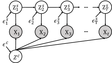
Figure 1: The generative process. The gray shade of nodes indicates that the variable is observable.

As shown in Figure 1 and Equation 1, the generative process is formulated as:

$$\left\{\begin{aligned} &{\mathbf{x}}_{t}=g({\mathbf{z}}_{t}^{s},{\mathbf{z}}^{c}),\\ &z_{t,i}^{s}=f^{s}_{i}\left(\mathbf{Pa}(z_{t,i}^{s}),\epsilon_{t,i}^{s}\right),\\ &z_{j}^{c}={f^{c}_{j}\left(\epsilon_{j}^{c}\right)},\end{aligned}\right.\text{with}\left\{\begin{aligned} \epsilon^{s}_{t,i}\sim p^{s}_{\epsilon_{i}},\\ \epsilon^{c}_{j}\sim p^{c}_{\epsilon_{j}},\end{aligned}\right.$$ (1)

in which $z_{t,i}^{s},z_{i}^{c}\in\mathbb{R}$ refers to the $i$-th entry of ${\mathbf{z}}_{t}^{s}$ and $j$-th entry of ${\mathbf{z}}^{c}$, respectively. $\mathbf{Pa}(z_{t,i}^{s})$ refers to the time-daleyed parents of $z_{t,i}^{s}$. All noise terms $\epsilon_{t,i}$ and $\epsilon_{j}$ are independently sampled from their respective distributions: $p_{\epsilon_{i}}^{s}$ for the $i$-th entry of the style dynamics, and $p_{\epsilon_{j}}^{c}$ for the $j$-th entry of the content elements. The components of ${\mathbf{z}}_{t}^{s}$ are mutually independent, conditioned on all historical variables $\cup_{i=1}^{n_{s}}\mathbf{Pa}(z_{t,i}^{s})$. The non-parametric causal transition $f_{i}$ enables an arbitrarily nonlinear interaction between the noise term $\epsilon_{t,i}$ and the set of parent variables $\mathbf{Pa}(z_{t,i}^{s})$, allowing for flexible modeling of the style dynamics.

3.2 Identification of the Latent Causal Process

For simplicity, we denote $\textbf{f}^{s}$ as the group of functions $\{f^{s}_{i}\}_{i=1}^{n_{s}}$, and similarly for $\textbf{f}^{c},\textbf{p}^{s},\textbf{p}^{c}$.

Definition 3.1 (Observational equivalence).

Let $V=\{{\mathbf{x}}_{1},{\mathbf{x}}_{2},\cdots,{\mathbf{x}}_{T}\}$ represent the observed video generated by the true generative process specified by $(g,\textbf{f}^{s},\textbf{f}^{c},\textbf{p}^{s},\textbf{p}^{c})$, as defined in Equation 1. A learned generative model $(\hat{g},\hat{\textbf{f}}^{s},\hat{\textbf{f}}^{c},\hat{\textbf{p}}^{s},\hat{\textbf{p}}^{c})$ is observationally equivalent to the true process if the model distribution $p_{(\hat{g},\hat{\textbf{f}}^{s},\hat{\textbf{f}}^{c},\hat{\textbf{p}}^{s},\hat{\textbf{p}}^{c})}(V)$ matches the data distribution $p_{(g,\textbf{f}^{s},\textbf{f}^{c},\textbf{p}^{s},\textbf{p}^{c})}(V)$ for all values of $V$.

Illustration. When observational equivalence is achieved, the distribution of videos generated by the model exactly matches that of the ground truth, i.e., the training set. In other words, the model produces video data that is indistinguishable from the actual observed data.

Definition 3.2 (Blockwise Identification of Generative Process).

Let the true generative process be $(g,\textbf{f}^{s},\textbf{f}^{c},\textbf{p}^{s},\textbf{p}^{c})$ as specified in Equation 1 and let its estimation be $(\hat{g},\hat{\textbf{f}}^{s},\hat{\textbf{f}}^{c},\hat{\textbf{p}}^{s},\hat{\textbf{p}}^{c})$. The generative process is identifiable up to the subspace of style dynamics and content elements, if the observational equivalence ensures that the estimated $(\hat{{\mathbf{z}}}_{t}^{s},\hat{{\mathbf{z}}}^{c})$ satisfies the condition that there exist bijective mappings from $(\hat{{\mathbf{z}}}_{t}^{s},\hat{{\mathbf{z}}}^{c})$ to $({\mathbf{z}}_{t}^{s},{\mathbf{z}}^{c})$ and from $\hat{{\mathbf{z}}}^{c}$ to ${\mathbf{z}}^{c}$. Formally, there exists invertible functions $h:\mathbb{R}^{n_{s}+n_{c}}\rightarrow\mathbb{R}^{n_{s}+n_{c}}$ and $h_{c}:\mathbb{R}^{n_{c}}\rightarrow\mathbb{R}^{n_{c}}$ such that

$$\ \ p_{(\hat{g},\hat{\textbf{f}}^{s},\hat{\textbf{f}}^{c},\hat{\textbf{p}}^{s},\hat{\textbf{p}}^{c})}(V)=p_{(g,\textbf{f}^{s},\textbf{f}^{c},\textbf{p}^{s},\textbf{p}^{c})}(V)$$ (2)

$$\Rightarrow \ \ [{\mathbf{z}}_{t}^{s},{\mathbf{z}}^{c}]=h([\hat{{\mathbf{z}}}_{t}^{s},\hat{{\mathbf{z}}}^{c}]),{\mathbf{z}}^{c}=h_{c}(\hat{{\mathbf{z}}}^{c}),$$

where $[\cdot]$ denotes concatenation.

Illustration. When blockwise identification is achieved, content elements are effectively disentangled. As a result, motion control can be applied independently, allowing manipulation of motion without altering the video’s content. For example, in a video where a camera moves forward, it becomes easy to change the camera’s direction without affecting the scene itself.

Definition 3.3 (Component-wise Identification of Style Dynamics).

On top of Definition 3.2, when $h^{s}$ is a combination of permutation $\pi$ and a component-wise invertible transformation $\mathcal{T}$. Formally,

$$\ \ p_{(\hat{g},\hat{\textbf{f}}^{s},\hat{\textbf{f}}^{c},\hat{\textbf{p}}^{s},\hat{\textbf{p}}^{c})}(V)=p_{(g,\textbf{f}^{s},\textbf{f}^{c},\textbf{p}^{s},\textbf{p}^{c})}(V)$$ (3)

$$\Rightarrow \ \ {\mathbf{z}}_{t}^{s}=(\pi\cdot\mathcal{T})(\hat{g}^{-1}_{s}({\mathbf{x}}_{t})).$$

Illustration. Achieving component-wise identification ensures that each estimated style variable corresponds exactly to one true style variable, which facilitates the disentangling of motion features. This enables efficient and precise control over video generation. For example, when generating a video of a person’s face, one can control different aspects, such as head movements or eye blinks, by adjusting the corresponding variables.

4 Theoritical Analysis

In this section, we discuss the conditions under which the blockwise identification (Definition 3.2) and component-wise identification (Definition 3.3) hold.

4.1 Blockwise Identification

Without loss of generality, we first consider the case where $\text{Pa}(z_{t,i}^{s})={\mathbf{z}}_{t-1}^{s}$, meaning that the time-dependent effects are governed by the dynamics of the previous time step.

Definition 4.1.

(Linear Operator) Consider two random variables $a$ and $b$ with support $\mathcal{A}$ and $\mathcal{B}$, the linear operator $L_{b\mid a}$ is defined as a mapping from a density function $p_{a}$ in some function space $\mathcal{F}(\mathcal{A})$ onto the density function $L_{b\mid a}\circ p_{a}$ in some function space $\mathcal{F}(\mathcal{B})$,

$$\mathcal{F}(\mathcal{A})\rightarrow\mathcal{F}(\mathcal{B}):\ p_{b}=L_{b\mid a}\circ p_{a}=\int_{\mathcal{A}}p_{b\mid a}(\cdot\mid a)p_{a}(a)da.$$

Theorem 4.2 (Blockwise Identifiability).

Consider video observation $V=\{{\mathbf{x}}_{1},{\mathbf{x}}_{2},\dots,{\mathbf{x}}_{T}\}$ generated by process $(g,\textbf{f}^{s},\textbf{f}^{c},\textbf{p}^{s},\textbf{p}^{c})$ with latent variables denoted as ${\mathbf{z}}_{t}^{s}$ and ${\mathbf{z}}_{c}$, according to Equation 1, where ${\mathbf{x}}_{t}\in\mathbb{R}^{n_{x}},{\mathbf{z}}_{t}^{s}\in\mathbb{R}^{n_{s}},{\mathbf{z}}^{c}\in\mathbb{R}^{n_{c}}$. If assumptions

• B1 (Positive Density) the probability density function of latent variables is always positive and bounded;

• B2 (Minimal Changes) the linear operators $L_{{\mathbf{x}}_{t+1}\mid{\mathbf{z}}_{t}^{s},{\mathbf{z}}^{c}}$ and $L_{{\mathbf{x}}_{t-1}\mid{\mathbf{x}}_{t+1}}$ are injective for bounded function space;

• B3 (Weakly Monotonic) for any $\dot{\mathbf{z}}_{t},\ddot{\mathbf{z}}_{t}\in\mathcal{Z}^{c}\times\mathcal{Z}^{s}_{t}$ $(\dot{\mathbf{z}}_{t}\neq\ddot{\mathbf{z}}_{t})$, the set $\{\mathbf{x}_{t}:p(\mathbf{x}_{t}|\dot{\mathbf{z}}_{t})\neq p(\mathbf{x}_{t}|\ddot{\mathbf{z}}_{t})\}$ has positive probability, and conditional densities are bounded and continuous;

• B4 (Blockwise Independence) the learned $\hat{{\mathbf{z}}}_{t}^{s}$ is independent with $\hat{{\mathbf{z}}}^{c}$;

are satisfied, then ${\mathbf{z}}_{t}$ is blockwisely identifiable with regard to $\hat{{\mathbf{z}}}_{t}$ from learned model $(\hat{g},\hat{\textbf{f}}^{s},\hat{\textbf{f}}^{c},\hat{\textbf{p}}^{s},\hat{\textbf{p}}^{c})$ under Observation Equivalence.

Illustration of Assumptions. The assumptions above are commonly used in the literature on the identification of latent variables under measurement error (Hu & Schennach, 2008). Firstly, Assumption B1 requires a continuous distribution. Secondly, Assumption B2 imposes a minimal requirement on the number of variables. The linear operator $L_{b|a}$ ensures that there is sufficient variation in the density of $b$ for different values of $a$, thereby guaranteeing injectivity. In a video, ${\mathbf{x}}_{t}$ is of much higher dimensionality compared to the latent variables. As a result, the injectivity assumption is easily satisfied. In practice, following the principle of minimal changes, if a model with fewer latent variables can successfully achieve observational equivalence, it is more likely to learn the true distribution. Assumption B3 requires the distribution of ${\mathbf{x}}_{t}$ changes when the value of latent variables changes. This assumption is much weaker compared to the widely used invertibility assumption adopted by previous works, such as (Yao et al., 2022). Assumption B4 requires that the learned latent variables have independent style dynamics and content elements.

Overall, the first three assumptions about the data are easily satisfied in real-world video scenarios. The last assumption, however, is a requirement for models. Most models that explicitly separate motion and identity satisfy this assumption.

Proof Sketch. We separately prove the identifiability of all latent variables and ${\mathbf{z}}^{c}$. For the first part, it is built on (Fu et al., 2025), following the line of work from (Hu & Schennach, 2008). Intuitively, it demonstrates that a minimum of 3 different observations of latent variables are required for identification under the given data generation process. For the second part, we use the contradiction to show that the same ${\mathbf{z}}^{c}$ in different frames of a video can be identified leveraging the invariance.

4.2 Component-wise Identification

Theorem 4.3 (Component-wise Identifiability).

Consider video observation $V=\{{\mathbf{x}}_{1},{\mathbf{x}}_{2},\dots,{\mathbf{x}}_{T}\}$ generated by process $(g,\textbf{f}^{s},\textbf{f}^{c},\textbf{p}^{s},\textbf{p}^{c})$ with latent variables denoted as ${\mathbf{z}}_{t}^{s}$ and ${\mathbf{z}}_{c}$, according to Equation 1, where ${\mathbf{x}}_{t}\in\mathbb{R}^{n_{x}},{\mathbf{z}}_{t}^{s}\in\mathbb{R}^{n_{s}},{\mathbf{z}}^{c}\in\mathbb{R}^{n_{c}}$. Suppose assumptions in Theorem 4.2 hold. If assumptions

• C1 (Smooth and Positive Density) the probability density function of latent variables is always third-order differentiable and positive;

• C2 (Sufficient Changes) let $\eta_{t,i}\triangleq\log p(z^{s}_{t,i}|{\mathbf{z}}_{t-1}^{s})$ and

  $$\mathbf{v}_{t,l} \triangleq\Big{(}\frac{\partial^{2}\eta_{t,1}}{\partial z_{t,1}\partial z_{t-1,l}},\cdots,\frac{\partial^{2}\eta_{t,n_{s}}}{\partial z_{t,n}\partial z_{t-1,l}}\Big{)}$$ (4)

  $$\oplus\Big{(}\frac{\partial^{3}\eta_{t,1}}{\partial^{2}z_{t,1}\partial z_{t-1,l}},\cdots,\frac{\partial^{3}\eta_{t,n_{s}}}{\partial^{2}z_{t,n}\partial z_{t-1,l}}\Big{)},$$

  for $l\in\{1,2,\cdots,n\}$. For each value of ${\mathbf{z}}_{t}$, there exists $2n_{s}$ different of values of $z_{t-1,l}$ such that the $2n_{s}$ vector ${\mathbf{v}}_{t,l}\in\mathbb{R}^{2n_{s}}$ are linearly independent;

• C3 (Conditional Independence) the learned $\hat{{\mathbf{z}}}_{t}^{s}$ is independent with $\hat{{\mathbf{z}}}^{c}$, and all entries of $\hat{{\mathbf{z}}}_{t}^{s}$ are mutually independent conditioned on $\hat{{\mathbf{z}}}_{t-1}^{s}$;

are satisfied, then ${\mathbf{z}}_{t}^{s}$ is component-wisely identifiable with regard to $\hat{{\mathbf{z}}}_{t}^{s}$ from learned model $(\hat{g},\hat{\textbf{f}}^{s},\hat{\textbf{f}}^{c},\hat{\textbf{p}}^{s},\hat{\textbf{p}}^{c})$ under Observation Equivalence.

Proof Sketch. In summary, component-wise identification relies on the changeability of style dynamics, i.e., sufficient changes. Starting from the results of blockwise identification, we establish the connection between ${\mathbf{z}}_{t}^{s}$ and $\hat{{\mathbf{z}}}_{t}^{s}$ in terms of their distributions, i.e., $p({\mathbf{z}}_{t})=p(\hat{{\mathbf{z}}}_{t})\cdot|H_{t}|$, where $H_{t}$ is the jacobian matrix. Leveraging the second-order derivative of the log probability, we construct a system of equations with terms of $\frac{\partial z_{t,i}^{s}}{\partial\hat{z}_{t,j}^{s}}\cdot\frac{\partial z_{t,i}^{s}}{\partial\hat{z}_{t,k}^{s}}$ and coefficients as specified in assumption C2. We leverage the third-order derivative of the previous latent variable $z_{t-1,l}$ to eliminate $|H_{t}|$, utilizing the fact that the history does not influence the current mapping from estimation to truth. Solving this system yields $\frac{\partial z_{t,i}^{s}}{\partial\hat{z}_{t,j}^{s}}\cdot\frac{\partial z_{t,i}^{s}}{\partial\hat{z}_{t,k}^{s}}=0$.

Illustration of Assumptions. The assumptions C1 and C2 on the data generative process are commonly adopted in existing identifiable results for Temporally Causal Representation Learning (Yao et al., 2022). Specifically, C1 implies that the latent variables evolve continuously over time, while C2 ensures that the variability in the data can be effectively captured. The assumption C3 constraints to the learned model requires it to separate different variables of style dynamics into independent parts.

5 Approach

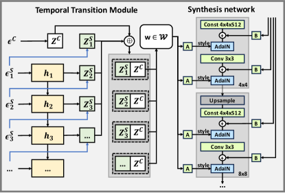
Figure 2: The workflow of the Generator proceeds from left to right, starting with random noise. It first passes through a Temporal Transition Module to obtain a disentangled representation, which is then fed into the synthesis network for frame-level generation. The blue arrow in the figure represents a component-wise flow.

Given our results on identifiability, we implement our model, CoVoGAN. Our architecture is based on StyleGAN2-ADA (Skorokhodov et al., 2022), incorporating a Temporal Transition Module in the Generator to enforce the minimal change principle and sufficient change property. Additionally, we add a Video Discriminator to ensure observational equivalence of the joint distribution $p(V)$.

5.1 Model Structure

Noise Sampling. The structure of the generator is shown in Figure 2. To generate a video with length $T$, we first independently sample random noise from a normal distribution $\epsilon\sim\mathcal{N}(\mathbf{0},\mathbf{I})$. We then naively split them into several parts, i.e., $\epsilon=[\epsilon^{c};\epsilon^{s}_{1};\epsilon^{s}_{2};\cdots;\epsilon^{s}_{T}]$.

Temporal Transition Module. Following the generative process in Equation 1, we handle ${\mathbf{z}}^{c}$ and ${\mathbf{z}}_{t}^{s}$ separately. On the one hand, we employ an autoregressive model to capture historical information, followed by a conditional flow to generate ${\mathbf{z}}_{t}^{s}$. Specifically, we implement a Gated Recurrent Unit (GRU) (Chung et al., 2014) and Deep Sigmoid Flow (DSF) (Huang et al., 2018), formulated as

$${\mathbf{h}}_{t}=\text{GRU}({\mathbf{h}}_{t-1},\epsilon_{t}^{s}),z_{t,i}^{s}=\text{DSF}_{i}(\epsilon_{t,i}^{s};{\mathbf{h}}_{t-1}).$$ (5)

On the other hand, since ${\mathbf{z}}^{c}$ are not required to be mutually independent, we use an MLP to generate ${\mathbf{z}}^{c}$, i.e.,

$${\mathbf{z}}^{c}=\text{MLP}(\epsilon^{c}).$$ (6)

Concatenate ${\mathbf{z}}_{t}^{s}$ and ${\mathbf{z}}^{c}$, and then we obtain the disentangled representation ${\mathbf{z}}_{t}={\mathbf{z}}^{c}\oplus{\mathbf{z}}_{t}^{s}$ for each frame at time step $t$ of the video.

Synthesis Network. The synthesis network is designed in the same way as StyleGAN2-ADA. The generated representation ${\mathbf{z}}_{t}$ is first fed into the mapping network to obtain a semantic vector $w({\mathbf{z}}_{t})\in\mathcal{W}$, and then the $t$-th frame of the video is generated by the convolutional network with $w$.

Discriminator Structure. To ensure observational equivalence, we implement a video discriminator $D_{V}$ separate from the image discriminator $D_{I}$. For the image discriminator, we follow the design of the original StyleGAN2-ADA. For the video discriminator, we adopt a channel-wise concatenation of activations at different resolutions to model and manage the spatiotemporal output of the generator.

Loss. In addition to the original loss function of StyleGAN2-ADA, we introduce two additional losses: (1) a video discriminator loss, and (2) a mutual information maximization term (Chen et al., 2016) between the latent dynamic variables ${\mathbf{z}}_{t}^{s}$ and the intermediate layer outputs of the video discriminator. This encourages the model to learn a more informative and structured representation.

5.2 Relationship between Model and Theorem.

In this subsection, we discuss the relationship between the CoVoGAN  model and the Theorem.

Blockwise Identification. As discussed in Theorem 4.2, achieving blockwise identifiability benefits from minimizing the dimension $n_{s}$ of the style dynamics, especially when the true $n_{s}$ is unknown. In practice, this translates to a hyperparameter selection question. In our experiments, we opted for a relatively modest value of $n_{s}$ and observed that it suffices to attain a satisfactory level of disentanglement capability. Furthermore, as required by assumption B4, the learned variables $\hat{{\mathbf{z}}}_{t}^{s}$ and $\hat{{\mathbf{z}}}^{c}$ are blockwise independent, i.e., $\hat{{\mathbf{z}}}_{t}^{s}\perp\!\!\!\perp\hat{{\mathbf{z}}}^{c}$. This independence is necessary to achieve blockwise identifiability.

Componenetwise Identification. As outlined in Theorem 4.3, the sufficient change property is a critical assumption for achieving identifiability. To enforce temporally conditional independence, we employ a component-wise flow model that transforms a set of independent noise variables $\epsilon_{t}^{s}$ into the style dynamics, conditioned on historical information. Furthermore, the flow model is designed to maximally preserve the information from $\epsilon_{t,i}^{s}$ to $z_{t,i}^{s}$, enabling the model to effectively capture sufficient variability in the data.

Note that when computing the historical information $h_{t}$, we utilize $\epsilon_{t}^{s}$ instead of ${\mathbf{z}}_{t}^{s}$ (as illustrated in the generative process in Equation 1) as the condition for the component-wise flow. This approach offers two key advantages. First, it simplifies the model architecture since the flow does not need to incorporate the output from another flow. Second, the noise terms already fully characterize the corresponding style dynamics, which remains consistent with the theoretical framework.

Furthermore, given that the precise time lag of dynamic variables remains unspecified a priori in the dataset, the GRU’s gating mechanism can selectively filter out irrelevant historical information that lies outside $\text{Pa}({\mathbf{z}}_{t})$. This capability enables the model to demonstrate significantly superior performance compared to traditional non-gated architectures, such as vanilla RNNs.

A detailed ablation study is presented in Section A4.1.

6 Experiments

In this section, we perform extensive experimental validation to comprehensively evaluate CoVoGAN. We design both qualitative and quantitative experiments to systematically assess the generation quality and controllability of our proposed model. Additionally, we conduct comparative studies to evaluate the robustness and computational efficiency of our model against state-of-the-art baselines. Finally, we perform comprehensive ablation studies to demonstrate the effectiveness of our proposed modules and analyze their individual contributions.

6.1 Experimental Setups

Datasets. We evaluate our model on three different real-world datasets: FaceForensics (Rössler et al., 2018), SkyTimelapse (Xiong et al., 2018), and RealEstate (Zhou et al., 2018). These datasets respectively capture dynamic variations in facial expressions, sky transitions, and complex camera movements, providing comprehensive evaluation scenarios for our method. FaceForensics and SkyTimelapse are widely adopted benchmarks in video generation research, particularly for facial manipulation and natural scene modeling. The RealEstate dataset contains video sequences featuring complex camera movements within static scenes. The camera motions in RealEstate are more intuitive and easily interpretable by human observers, including forward/backward movements, lateral shifts, etc. We particularly leverage this dataset to effectively demonstrate the precise controllability of CoVoGAN in handling explicit camera motion parameters. All datasets consist of videos with a resolution of 256 × 256 pixels, and we employ standard train-test splits for fair evaluation. Detailed statistics and additional information about the datasets are provided in Appendix A2.

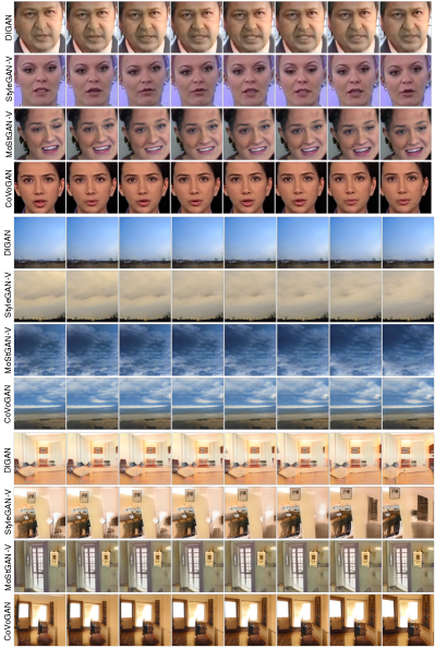
Figure 3: Random samples from the comparison baselines and our model on real-world datasets FaceForensics $256^{2}$, SkyTimelapse $256^{2}$, RealEstate $256^{2}$. Start from t = 0 and report every 2-nd frame from a 16-frame video clip.

Evaluation metrics. To comprehensively evaluate the performance of CoVoGAN, we employ both quantitative and qualitative assessment metrics. For quantitative evaluation, we adopt the Fréchet Video Distance (FVD) (Unterthiner et al., 2018), a widely-used metric for assessing video generation quality. FVD computes the Wasserstein-2 distance between feature distributions of real and generated videos in a learned feature space, providing a comprehensive measure of visual quality and temporal coherence. We report FVD scores at two different temporal scales: $\text{FVD}_{8}$ and $\text{FVD}_{16}$, where the subscript denotes the number of frames in a video. For qualitative evaluation, we present randomly sampled video sequences generated by our model.

6.2 Quality of the video.

We conduct comparisons between our proposed CoVoGAN and four baselines: MoCoGAN-HD, DIGAN, StyleGAN-V, and MoStGAN-V, across three benchmark datasets: FaceForensics, SkyTimelapse, and RealEstate. For MoCoGAN-HD, we utilize the image generator pretrained by the original authors and train the remaining components (including the motion generator and discriminator). Due to the unavailability of pretrained models for the RealEstate dataset, we exclude MoCoGAN-HD from the comparisons on this specific dataset. For the remaining baselines (DIGAN, StyleGAN-V, and MoSTGAN-V), we train the models from scratch using their official implementations to ensure comparability. The quantitative evaluation results, presented in Table 1, show that CoVoGAN consistently achieves superior performance across all datasets, with significantly lower FVD scores compared to the baseline methods. This improvement in FVD metrics demonstrates our model’s enhanced capability to generate high-quality, temporally coherent videos. Some randomly sampled videos are shown in Figure 3.

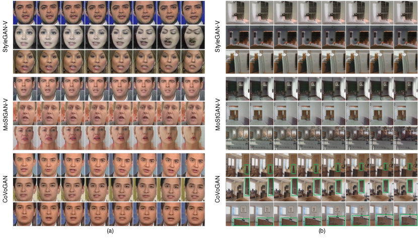
Figure 4: Generate same motion of different identities in (a) FaceForensics, (b) RealEstate.

Table 1: $\text{FVD}_{8}\downarrow$ and $\text{FVD}_{16}\downarrow$ scores across the FaceForensics, SkyTimelapse, and RealEstate datasets.

Method	FaceForensics $\text{256}^{2}$		SkyTimelapse $\text{256}^{2}$		RealEstate $\text{256}^{2}$
	$\text{FVD}_{8}$	$\text{FVD}_{16}$	$\text{FVD}_{8}$	$\text{FVD}_{16}$	$\text{FVD}_{8}$	$\text{FVD}_{16}$
MoCoGAN-HD	140.05	185.51	1214.13	1721.89	-	-
DIGAN	57.52	61.65	60.54	105.03	182.86	178.27
StyleGAN-V	49.24	52.70	45.30	62.55	199.66	201.95
MoStGAN-V	47.67	49.85	40.97	55.36	247.77	265.54
CoVoGAN (ours)	43.75	48.80	35.58	46.51	154.88	174.87

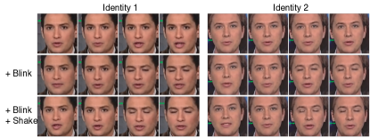
Figure 5: Controllability visualization results on the FaceForensics dataset. Two different concepts of motion is modified to show the component-wise level disentanglement. The fisrt line is a randomly sampled video, and the following lines apply control of eye blinking and head shaking.

6.3 Controllability

Blockwise Disentanglement. Figure 4 demonstrates the video controllability of CoVoGAN in comparison with baseline methods, highlighting our model’s superior capability of disentanglement between motion and content. The analysis follows a systematic procedure: we first generate a base video sequence, then apply a controlled modification by adding a value to specific motion-related latent variables.

For CoVoGAN, we modify one dimension of the style dynamics ${\mathbf{z}}_{t}^{s}$. For StyleGAN-V and MoStGAN-V, we manipulate one dimension of its (latent) motion code. We apply equivalent modifications to the corresponding latent dimensions in each baseline model. To validate the consistency of our controllability analysis, we randomly sample three distinct video sequences and apply identical modifications to their respective latent representations. DIGAN is not compared since there are no specific variables for motion.

The results show that our proposed CoVoGAN model learns a disentangled representation that effectively separates style dynamics from content elements. (1) This disentanglement enables independent manipulation of motion characteristics while preserving content consistency. (2) A key advantage of this approach is that identical modifications to the style latent space consistently produce similar motion patterns across different content identities.

Baseline models achieve only partial disentanglement, exhibiting two major limitations: (1) visual distortions of the modified videos and (2) inconsistent or misaligned motion patterns when applied to different identities.

Table 2: Comparison of different models in terms of generator parameters (Params, in millions) and the time (Time, in seconds) required to generate 16-frame 2048 videos with a resolution of $256\times 256$.

Method	Params (M)	Time (s)
StyleGAN2-ADA	23.19	-
DIGAN	69.97	142.06
StyleGAN-v	32.11	181.45
MoStGAN	40.92	207.11
CoVoGAN (ours)	24.98	98.93

Componenet-wise Disentanglement. We further illustrate the precise control over individual motion components. This capability is enabled by the component-wise identifiability of our model, which ensures that each latent dimension corresponds to a specific and interpretable motion attribute.

Our experimental procedure begins with randomly sampling two distinct video sequences, as illustrated in the first row of Figure 5. We then selectively modify the latent dimension corresponding to eye blinking dynamics in the second line. Subsequently, we modify a second latent dimension controlling head shaking motion while maintaining the previously adjusted eye blinking pattern in the last line. The results show naturalistic head movements from left to right, synchronized with the preserved eye blinking, illustrating our model’s capability for independent yet coordinated control of multiple motion components.

6.4 More Evaluations

Robustness. The architectural simplicity of CoVoGAN contributes to a more stable and efficient convergence compared to baseline models, as shown in Figure 6. Our model demonstrates faster convergence and greater stability, particularly on challenging noncenter-focused datasets such as RealEstate. These datasets are notoriously difficult for GAN-based approaches. Furthermore, CoVoGAN exhibits enhanced robustness against model collapse during the later stages of training, a common issue in adversarial training frameworks.

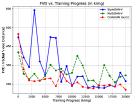
Figure 6: Comparisons of FVD variations during training steps (kimg) on RealEstate Dataset VS baselines.

Computational Efficiency. We also compare the computational efficiency with that of the baselines. The size of our model’s generator is comparable to that of StyleGAN2-ADA but significantly smaller than the generators of the baselines. Additionally, the inference time of our model is much faster, as shown in Table 2.

7 Conclusion

In this paper, we proposed a Temporal Transition Module and implemented it in a GAN to achieve CoVoGAN. By leveraging the principle of minimal and sufficient changes, we successfully disentangled (1) the motion and content of a video, and (2) different concepts within the motion. We established an identifiability guarantee for both blockwise and component-wise disentanglement. Our proposed CoVoGAN model demonstrates high generative quality, controllability, and a more robust and computationally efficient structure. We validated the performance on various datasets and conducted ablation experiments to further confirm the effectiveness of our model.

Impact Statements

This study introduces both a theoretical framework and a practical approach for extracting disentangled causal representations from videos. Such advancements enable the development of more transparent and interpretative models, enhancing our grasp of causal dynamics in real-world settings. This approach may benefit many real-world applications, including healthcare, auto-driving, content generation, marketing and so on.

Appendix A1 Identifiability Theory

Without loss of generality, we first consider the case where $\text{Pa}(z_{t,i}^{s})={\mathbf{z}}_{t-1}^{s}$, meaning that the time-dependent effects are governed by the dynamics of the previous time step.

Theorem A1 (Blockwise Identifiability).

Consider video observation $V=\{{\mathbf{x}}_{1},{\mathbf{x}}_{2},\dots,{\mathbf{x}}_{T}\}$ generated by process $(g,\textbf{f}^{s},\textbf{f}^{c},\textbf{p}^{s},\textbf{p}^{c})$ with latent variables denoted as ${\mathbf{z}}_{t}^{s}$ and ${\mathbf{z}}_{c}$, according to Equation 1, where ${\mathbf{x}}_{t}\in\mathbb{R}^{n_{x}},{\mathbf{z}}_{t}^{s}\in\mathbb{R}^{n_{s}},{\mathbf{z}}^{c}\in\mathbb{R}^{n_{c}}$. If assumptions

• B1 (Positive Density) the probability density function of latent variables is always positive and bounded;

• B2 (Minimal Changes) the linear operators $L_{{\mathbf{x}}_{t+1}\mid{\mathbf{z}}_{t}^{s},{\mathbf{z}}^{c}}$ and $L_{{\mathbf{x}}_{t-1}\mid{\mathbf{x}}_{t+1}}$ are injective for bounded function space;

• B3 (Weakly Monotonic) for any $\dot{\mathbf{z}}_{t},\ddot{\mathbf{z}}_{t}\in\mathcal{Z}^{c}\times\mathcal{Z}^{s}_{t}$ $(\dot{\mathbf{z}}_{t}\neq\ddot{\mathbf{z}}_{t})$, the set $\{\mathbf{x}_{t}:p(\mathbf{x}_{t}|\dot{\mathbf{z}}_{t})\neq p(\mathbf{x}_{t}|\ddot{\mathbf{z}}_{t})\}$ has positive probability, and conditional densities are bounded and continuous;

are satisfied, then ${\mathbf{z}}_{t}$ is blockwisely identifiable with regard to $\hat{{\mathbf{z}}}_{t}$ from learned model $(\hat{g},\hat{\textbf{f}}^{s},\hat{\textbf{f}}^{c},\hat{\textbf{p}}^{s},\hat{\textbf{p}}^{c})$ under Observation Equivalence.

Proof.

We first prove the monoblock identification of ${\mathbf{z}}_{t}^{s},{\mathbf{z}}^{c}=h(\hat{{\mathbf{z}}}_{t}^{s},\hat{{\mathbf{z}}}^{c})$, then we prove the blockwise identification ${\mathbf{z}}^{c}=h_{c}(\hat{{\mathbf{z}}}^{c})$.

Monoblock Identification. Following (Hu & Shum, 2012; Hu & Schennach, 2008), when assumptions B1, B2, B3 satisfied, the blockwise identifiability of $[{\mathbf{z}}_{t}^{s},{\mathbf{z}}^{c}]$ is assured, according to Theorem 3.2(Monoblock identifiability) in (Fu et al., 2025). In short ,there exists a invertible function $g$ such that $[{\mathbf{z}}_{t}^{s},{\mathbf{z}}^{c}]=h(\hat{{\mathbf{z}}}_{t}^{s},\hat{{\mathbf{z}}}^{c})$, where $[\cdot]$ denotes concatenation.

Identification of ${\mathbf{z}}^{c}$. We prove this by contradiction. Suppose that for any $\hat{{\mathbf{z}}}^{c}$, we have

$${\mathbf{z}}^{c}=h_{c}(\hat{{\mathbf{z}}}_{t}^{s},\hat{{\mathbf{z}}}^{c}),$$ (A1)

where there exist at least two distinct values of $\hat{{\mathbf{z}}}_{t}^{s}$ such that ${\mathbf{z}}^{c}$ takes different values.

When observational equivalence holds, the function remains the same for all values of $t$:

$$h_{c}(\hat{{\mathbf{z}}}_{t}^{s},\hat{{\mathbf{z}}}^{c})=g_{c}^{-1}({\mathbf{x}}_{t})=(g_{c}^{-1}\circ\hat{g})(\hat{{\mathbf{z}}}_{t}^{s},\hat{{\mathbf{z}}}^{c}),$$ (A2)

where $g_{c}^{-1}$ first demix ${\mathbf{x}}_{t}$ then extract the content part, as defined in Equation 2.

For any two distinct $t\neq t^{\prime}$, we have

$$h_{c}(\hat{{\mathbf{z}}}_{t}^{s},\hat{{\mathbf{z}}}^{c})={\mathbf{z}}^{c}=h_{c}(\hat{{\mathbf{z}}}_{t^{\prime}}^{s},\hat{{\mathbf{z}}}^{c}),$$ (A3)

which holds for all pairs $(\hat{{\mathbf{z}}}_{t}^{s},\hat{{\mathbf{z}}}_{t^{\prime}}^{s})$ within the domain of definition.

According to Assumption B1, the joint distribution $p(\hat{{\mathbf{z}}}_{t}^{s},\hat{{\mathbf{z}}}_{t^{\prime}}^{s})$ is always positive. Thus, to satisfy Equation A3, $\hat{{\mathbf{z}}}_{t}^{s}$ must not contribute to ${\mathbf{z}}^{c}$ through $h_{c}$. In other words, we obtain

$${\mathbf{z}}^{c}=h_{c}(\hat{{\mathbf{z}}}^{c}).$$ (A4)

∎

Theorem A2 (Component-wise Identifiability).

Consider video observation $V=\{{\mathbf{x}}_{1},{\mathbf{x}}_{2},\dots,{\mathbf{x}}_{T}\}$ generated by process $(g,\textbf{f}^{s},\textbf{f}^{c},\textbf{p}^{s},\textbf{p}^{c})$ with latent variables denoted as ${\mathbf{z}}_{t}^{s}$ and ${\mathbf{z}}_{c}$, according to Equation 1, where ${\mathbf{x}}_{t}\in\mathbb{R}^{n_{x}},{\mathbf{z}}_{t}^{s}\in\mathbb{R}^{n_{s}},{\mathbf{z}}^{c}\in\mathbb{R}^{n_{c}}$. Suppose assumptions in Theorem A1 hold. If assumptions

• C1 (Smooth and Positive Density) the probability density function of latent variables is always third-order differentiable and positive;

• C2 (Sufficient Changes) let $\eta_{t,i}\triangleq\log p(z^{s}_{t,i}|{\mathbf{z}}_{t-1}^{s})$ and

  $$\mathbf{v}_{t,l}\triangleq\Big{(}\frac{\partial^{2}\eta_{t,1}}{\partial z_{t,1}\partial z_{t-1,l}},\cdots,\frac{\partial^{2}\eta_{t,n_{s}}}{\partial z_{t,n}\partial z_{t-1,l}}\Big{)}\oplus\Big{(}\frac{\partial^{3}\eta_{t,1}}{\partial^{2}z_{t,1}\partial z_{t-1,l}},\cdots,\frac{\partial^{3}\eta_{t,n_{s}}}{\partial^{2}z_{t,n}\partial z_{t-1,l}}\Big{)},$$ (A5)

  for $l\in\{1,2,\cdots,n\}$. For each value of ${\mathbf{z}}_{t}$, there exists $2n_{s}$ different of values of $z_{t-1,l}$ such that the $2n_{s}$ vector ${\mathbf{v}}_{t,l}\in\mathbb{R}^{2n_{s}}$ are linearly independent;

• C3 (Conditional Independence) the learned $\hat{{\mathbf{z}}}_{t}^{s}$ is independent with $\hat{{\mathbf{z}}}^{c}$, and all entries of $\hat{{\mathbf{z}}}_{t}^{s}$ are mutually independent conditioned on $\hat{{\mathbf{z}}}_{t-1}^{s}$;

are satisfied, then ${\mathbf{z}}_{t}^{s}$ is component-wisely identifiable with regard to $\hat{{\mathbf{z}}}_{t}^{s}$ from learned model $(\hat{g},\hat{\textbf{f}}^{s},\hat{\textbf{f}}^{c},\hat{\textbf{p}}^{s},\hat{\textbf{p}}^{c})$ under Observation Equivalence.

Proof.

According to Theorem A1, we have

$$[{\mathbf{z}}_{t}^{s},{\mathbf{z}}^{c}]=h([\hat{\mathbf{z}}_{t}^{s},\hat{\mathbf{z}}^{c}]),$$ (A6)

where $[.]$ denotes the concatenation operation. The corresponding Jacobian matrix can be formulated as

$$H_{t}=\begin{bmatrix}\frac{\partial{\mathbf{z}}_{t}^{s}}{\partial\hat{\mathbf{z}}_{t}^{s}}&\frac{\partial{\mathbf{z}}^{c}}{\partial\hat{\mathbf{z}}_{t}^{s}}\\ \frac{\partial{\mathbf{z}}_{t}^{s}}{\partial\hat{\mathbf{z}}^{c}}&\frac{\partial{\mathbf{z}}^{c}}{\partial\hat{\mathbf{z}}^{c}}\end{bmatrix}.$$ (A7)

Consider a mapping from $({\mathbf{x}}_{t-1},\hat{{\mathbf{z}}}_{t}^{s},\hat{{\mathbf{z}}}^{c})$ to $({\mathbf{x}}_{t-1},{\mathbf{z}}_{t}^{s},{\mathbf{z}}^{c})$ and its Jacobian matrix

$$\begin{bmatrix}\mathbf{I}&\mathbf{0}\\ \mathbf{*}&H_{t}\end{bmatrix},$$ (A8)

where $*$ stands for any matrix, and the absolute value of the determination of this Jacobian is $|H_{t}|$. Therefore $p({\mathbf{x}}_{t-1},{\mathbf{z}}_{t}^{s},{\mathbf{z}}^{c})=p({\mathbf{x}}_{t-1},\hat{{\mathbf{z}}}_{t}^{s},\hat{{\mathbf{z}}}^{c})/|H_{t}|$. Dividing both side by $p({\mathbf{x}}_{t-1})$ gives

$$\begin{aligned} &&p({\mathbf{z}}_{t}^{s},{\mathbf{z}}^{c}|{\mathbf{x}}_{t-1})&=p(\hat{{\mathbf{z}}}_{t}^{s},\hat{{\mathbf{z}}}^{c}|{\mathbf{x}}_{t-1})/|H_{t}|\\ &\Rightarrow&p({\mathbf{z}}_{t}^{s},{\mathbf{z}}^{c}|g({\mathbf{z}}_{t-1}^{s},{\mathbf{z}}^{c}))&=p(\hat{{\mathbf{z}}}_{t}^{s},\hat{{\mathbf{z}}}^{c}|\hat{g}(\hat{{\mathbf{z}}}_{t-1}^{s},\hat{{\mathbf{z}}}^{c}))/|H_{t}|\\ &\Rightarrow&p({\mathbf{z}}_{t}^{s},{\mathbf{z}}^{c}|{\mathbf{z}}_{t-1}^{s},{\mathbf{z}}^{c})&=p(\hat{{\mathbf{z}}}_{t}^{s},\hat{{\mathbf{z}}}^{c}|\hat{{\mathbf{z}}}_{t-1}^{s},\hat{{\mathbf{z}}}^{c})/|H_{t}|\\ &\Rightarrow&p({\mathbf{z}}_{t}^{s}|{\mathbf{z}}_{t-1}^{s},{\mathbf{z}}^{c})&=p(\hat{{\mathbf{z}}}_{t}^{s}|\hat{{\mathbf{z}}}_{t-1}^{s},\hat{{\mathbf{z}}}^{c})/|H_{t}|\\ &\Rightarrow&p({\mathbf{z}}_{t}^{s}|{\mathbf{z}}_{t-1}^{s})&=p(\hat{{\mathbf{z}}}_{t}^{s}|\hat{{\mathbf{z}}}_{t-1}^{s})/|H_{t}|\\ \end{aligned}.$$ (A9)

For the first two implications, we utilize the inversion of the mixing function to replace the condition. For the third, since ${\mathbf{z}}^{c}$ is conditioned on itself, it remains fixed. For the last one, given that in the generative process, $\epsilon_{t,i}^{s}$ and $\epsilon_{j}^{c}$ for all $i,j,t$ are independently sampled, their disjoint successors are also independent, i.e., ${\mathbf{z}}_{t}^{s}\perp{\mathbf{z}}^{c}$. Similarly, following assumption C3, we have $\hat{{\mathbf{z}}}_{t}^{s}\perp\hat{{\mathbf{z}}}^{c}$. Thus, we can remove ${\mathbf{z}}^{c}$ from the condition.

For simplicity, denote $\mathbb{\eta}_{t}\triangleq\log p({\mathbf{z}}^{s}_{t}|{\mathbf{z}}_{t-1}^{s})$ and $\eta_{t,i}\triangleq\log p(z^{s}_{t,i}|{\mathbf{z}}_{t-1}^{s})$ and we have

$$\mathbb{\eta}_{t}=\hat{\mathbb{\eta}}_{t}-\log|H_{t}|.$$ (A10)

For any two different $\hat{z}_{t,i}^{s},\hat{z}_{t,j}^{s}\in{\mathbf{z}}_{t}^{s}$, in partial derivative with regard to $\hat{z}_{t,i}^{s}$ gives

$$\sum_{k=1}^{n_{s}}\frac{\partial\mathbb{\eta}_{t}}{\partial z_{t,k}^{s}}\cdot\frac{\partial z_{t,k}^{s}}{\partial\hat{z}_{t,i}^{s}}=\frac{\partial\hat{\mathbb{\eta}}_{t}}{\partial\hat{z}_{t,i}^{s}}-\frac{\partial\log|H_{t}|}{\partial\hat{z}_{t,i}^{s}}.$$ (A11)

Reorganize the left-hand side of Equation A11 with mutual independence of ${\mathbf{z}}_{t}^{s}|{\mathbf{z}}_{t-1}^{s}$ yields

$$\sum_{k=1}^{n_{s}}\frac{\partial\mathbb{\eta}_{t}}{\partial z_{t,k}^{s}}\cdot\frac{\partial z_{t,k}^{s}}{\partial\hat{z}_{t,i}^{s}}=\sum_{k=1}^{n_{s}}\frac{\partial\prod_{k^{\prime}=1}^{n_{s}}\eta_{t,k^{\prime}}}{\partial z_{t,k}^{s}}\cdot\frac{\partial z_{t,k}^{s}}{\partial\hat{z}_{t,i}^{s}}=\sum_{k=1}^{n_{s}}\frac{\partial\eta_{t,k}}{\partial z_{t,k}^{s}}\cdot\frac{\partial z_{t,k}^{s}}{\partial\hat{z}_{t,i}^{s}},$$ (A12)

and we have

$$\sum_{k=1}^{n_{s}}\frac{\partial\eta_{t,k}}{\partial z_{t,k}^{s}}\cdot\frac{\partial z_{t,k}^{s}}{\partial\hat{z}_{t,i}^{s}}=\frac{\partial\hat{\mathbb{\eta}}_{t}}{\partial\hat{z}_{t,i}^{s}}-\frac{\partial\log|H_{t}|}{\partial\hat{z}_{t,i}^{s}}.$$ (A13)

Further get the second-order derivative with regard to $\hat{z}_{t,j}^{s}$ as

$$\sum_{k=1}^{n_{s}}\frac{\partial^{2}\eta_{t,k}}{\partial^{2}z_{t,k}^{s}}\cdot\frac{\partial z_{t,k}^{s}}{\partial\hat{z}_{t,i}^{s}}\cdot\frac{\partial z_{t,k}^{s}}{\partial\hat{z}_{t,j}^{s}}+\sum_{k=1}^{n_{s}}\frac{\partial\eta_{t,k}}{\partial z_{t,k}^{s}}\cdot\frac{\partial^{2}z_{t,k}^{s}}{\partial\hat{z}_{t,i}^{s}\partial\hat{z}_{t,j}^{s}}=\frac{\partial^{2}\hat{\mathbb{\eta}}_{t}}{\partial\hat{z}_{t,i}^{s}\partial\hat{z}_{t,j}^{s}}-\frac{\partial^{2}\log|H_{t}|}{\partial\hat{z}_{t,i}^{s}\partial\hat{z}_{t,j}^{s}}.$$ (A14)

Next, using the mutual independence of $\hat{{\mathbf{z}}}_{t}^{s}|\hat{{\mathbf{z}}}_{t-1}^{s}$ in assumption C3, we have $\frac{\partial^{2}\hat{\mathbb{\eta}}_{t}}{\partial\hat{z}_{t,i}^{s}\partial\hat{z}_{t,j}^{s}}=0$ according to the connection between conditional independence and cross derivatives (Lin, 1997). Thus we have

$$\sum_{k=1}^{n_{s}}\frac{\partial^{2}\eta_{t,k}}{\partial^{2}z_{t,k}^{s}}\cdot\frac{\partial z_{t,k}^{s}}{\partial\hat{z}_{t,i}^{s}}\cdot\frac{\partial z_{t,k}^{s}}{\partial\hat{z}_{t,j}^{s}}+\sum_{k=1}^{n_{s}}\frac{\partial\eta_{t,k}}{\partial z_{t,k}^{s}}\cdot\frac{\partial^{2}z_{t,k}^{s}}{\partial\hat{z}_{t,i}^{s}\partial\hat{z}_{t,j}^{s}}=-\frac{\partial^{2}\log|H_{t}|}{\partial\hat{z}_{t,i}^{s}\partial\hat{z}_{t,j}^{s}}.$$ (A15)

Now we get the third-order derivative with regard to any $z_{t-1,l}^{s}$ as

$$\sum_{k=1}^{n_{s}}\frac{\partial^{3}\eta_{t,k}}{\partial^{2}z_{t,k}^{s}\partial z_{t-1,l}^{s}}\cdot\frac{\partial z_{t,k}^{s}}{\partial\hat{z}_{t,i}^{s}}\cdot\frac{\partial z_{t,k}^{s}}{\partial\hat{z}_{t,j}^{s}}+\sum_{k=1}^{n_{s}}\frac{\partial\eta_{t,k}}{\partial z_{t,k}^{s}}\cdot\frac{\partial^{2}z_{t,k}^{s}}{\partial\hat{z}_{t,i}^{s}\partial\hat{z}_{t,j}^{s}}=0,$$ (A16)

where we use the property that the entries of $H_{t}$ do not depend on $z_{t-1,l}^{s}$.

Given assumption C2, there exists $2n_{s}$ different values of $z_{t-1,l}^{s}$ such that the $2n_{s}$ vectors ${\mathbf{v}}_{t,l}$ linearly independent. The only solution to Equation A16 is to set

$$\frac{\partial z_{t,k}^{s}}{\partial\hat{z}_{t,i}^{s}}\cdot\frac{\partial z_{t,k}^{s}}{\partial\hat{z}_{t,j}^{s}}=0,\frac{\partial^{2}z_{t,k}^{s}}{\partial\hat{z}_{t,i}^{s}\partial\hat{z}_{t,j}^{s}}=0.$$ (A17)

According to Theorem A1, the blockwise identifiability is established. Thus,

$$H_{t}=\begin{bmatrix}\frac{\partial{\mathbf{z}}_{t}^{s}}{\partial\hat{\mathbf{z}}_{t}^{s}}&\frac{\partial{\mathbf{z}}^{c}}{\partial\hat{\mathbf{z}}_{t}^{s}}\\ \frac{\partial{\mathbf{z}}_{t}^{s}}{\partial\hat{\mathbf{z}}^{c}}&\frac{\partial{\mathbf{z}}^{c}}{\partial\hat{\mathbf{z}}^{c}}\end{bmatrix}$$ (A18)

is invertible, with $\frac{\partial{\mathbf{z}}^{c}}{\partial\hat{\mathbf{z}}_{t}^{s}}=0$ and $\frac{\partial{\mathbf{z}}_{t}^{s}}{\partial\hat{\mathbf{z}}_{t}^{s}}$ has at most one nonzero element in each row and each column.

Thus, we have

$$H_{t}=\begin{bmatrix}\frac{\partial{\mathbf{z}}_{t}^{s}}{\partial\hat{\mathbf{z}}_{t}^{s}}&0\\ \frac{\partial{\mathbf{z}}_{t}^{s}}{\partial\hat{\mathbf{z}}^{c}}&\frac{\partial{\mathbf{z}}^{c}}{\partial\hat{\mathbf{z}}^{c}}\end{bmatrix}$$ (A19)

and $\frac{\partial{\mathbf{z}}_{t}^{s}}{\partial\hat{\mathbf{z}}_{t}^{s}}$ must have one and only one non-zero entry in each column and row.

∎

Appendix A2 Datasets details

FaceForensics (Rössler et al., 2018) is a forensics dataset consisting of 1000 original video sequences all videos contain a trackable mostly frontal face without occlusions. SkyTimelapse (Xiong et al., 2018) typically consists of sequential images or videos capturing the dynamic behavior of the sky over time.

RealEstate10K (Zhou et al., 2018) is a large dataset of camera poses corresponding to 10 million frames derived from about 80,000 video clips, gathered from about 10,000 YouTube videos. For each clip, the poses form a trajectory where each pose specifies the camera position and orientation along the trajectory. These poses are derived by running SLAM and bundle adjustment algorithms on a large set of videos. To the best of our knowledge, the proposed method is the first GAN-based approach to leverage the complex camera pose dataset for validating unconditional video generation.

Appendix A3 Reproductability

All of our models are trained on an NVIDIA A100 40G GPU. For the baseline models, we use the official implementation with the default hyperparameters. The configuration of hyperparameters for our model training is as shown in Table  A1.

Table A1: Configuration details for the model and training setup.

Name	Variable Name	Value/Description
Information regularization term weight	lambda_KL	1
Dimensionality of ${\mathbf{z}}^{c}$	-	512
Dimensionality of GRU	-	64
Dimensionality of ${\mathbf{z}}_{s}^{t}$	-	FaceForensics: 4, SkyTimelapse: 12, RealEstate: 12
Batch size (per GPU)	batch	16
Conditional mode	cond_mode	flow
Flow normalization	flow_norm	1
Sparsity weight	lambda_sparse	0.1
Number of input channels	channel	3
Number of mapping layers	num_layers	8
Label embedding features	embed_features	512
Intermediate layer features	layer_features	512
Activation function	activation	lrelu
Learning rate multiplier	lr_multiplier	0.01
Moving average decay	w_avg_beta	0.995
Discriminator architecture	-	resnet
Channel base	channel_base	32768
Maximum number of channels	channel_max	512

The architecture of our proposed Temporal Transition Module is shown in Table A2.

Appendix A4 More experiments

A4.1 Ablation Study

An ablation study is conducted to assess the contribution of our proposed modules in the Temporal Transition Module, as shown in Table A3.

Table A2: Architecture of Temporal Transition Module

Component	Structure
MappingNetwork.gru	$4\times 256\times 3$
MappingNetwork.h_to_c	FullyConnectedLayer ($256\times 64$)
MappingNetwork.embed	FullyConnectedLayer ($64\times 512$)
MappingNetwork.flow.model.0	DenseSigmoidFlow
MappingNetwork.flow.model.1	DenseSigmoidFlow
MappingNetwork.flow_fc0	FullyConnectedLayer ($512\times 512$)
MappingNetwork.flow_fc1	FullyConnectedLayer ($512\times 512$)
MappingNetwork.flow_fc2	FullyConnectedLayer ($512\times 284$)
FullyConnectedLayer	FullyConnectedLayer ($512\times 512$)
FullyConnectedLayer	FullyConnectedLayer ($512\times 512$)

Replacing the GRU with an RNN results in a performance decline, as the sparsity of time-delayed effects—enabled by the gating mechanism—vanishes. This makes it more challenging for the model to learn a true transition function, as it must navigate a larger search space without sparsity constraints.

Replacing the component-wise flow with a fully connected MLP leads to an even greater performance drop in FVD because (1) the mutual independence between style dynamics can no longer be maintained, and (2) capturing sufficient changes becomes more difficult.

	w/ GRU, w/ Flow	w/o GRU	w/o Flow
$\text{FVD}_{16}$	48.80	53.68	82.81

Table A3: Ablation study results for different configurations of GRU and component-wise flow on the FaceForensics dataset.

A4.2 More Videos

In this section, we provide more qualitative video results generated by our approach. As can be seen in A1, our method can control different identities of sky scenes with consistent constructed motions.

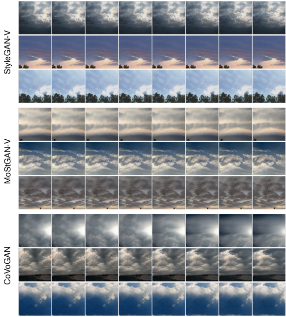
Figure A1: Generate same motion of different identities on SkyTimelapse Dataset.

References

- Cao et al. (2024) Cao, X., Liang, K., Liao, K.-D., Gao, T., Ye, W., Chen, J., Ding, Z., Cao, J., Rehg, J. M., and Sun, J. Medical video generation for disease progression simulation. arXiv preprint arXiv:2411.11943, 2024.
- Chen et al. (2024) Chen, G., Shen, Y., Chen, Z., Song, X., Sun, Y., Yao, W., Liu, X., and Zhang, K. Caring: Learning temporal causal representation under non-invertible generation process. arXiv preprint arXiv:2401.14535, 2024.
- Chen et al. (2016) Chen, X., Duan, Y., Houthooft, R., Schulman, J., Sutskever, I., and Abbeel, P. Infogan: Interpretable representation learning by information maximizing generative adversarial nets. Advances in neural information processing systems, 29, 2016.
- Chung et al. (2014) Chung, J., Gulcehre, C., Cho, K., and Bengio, Y. Empirical evaluation of gated recurrent neural networks on sequence modeling. arXiv preprint arXiv:1412.3555, 2014.
- Fei et al. (2024) Fei, H., Wu, S., Ji, W., Zhang, H., and Chua, T.-S. Dysen-vdm: Empowering dynamics-aware text-to-video diffusion with llms. In Proceedings of the IEEE/CVF Conference on Computer Vision and Pattern Recognition, pp. 7641–7653, 2024.
- Fu et al. (2025) Fu, M., Huang, B., Li, Z., Zheng, Y., Ng, I., Hu, Y., and Zhang, K. Identification of nonparametric dynamic causal structure and latent process in climate system. arXiv preprint arXiv:2501.12500, 2025.
- Ho et al. (2022) Ho, J., Salimans, T., Gritsenko, A., Chan, W., Norouzi, M., and Fleet, D. J. Video diffusion models. Advances in Neural Information Processing Systems, 35:8633–8646, 2022.
- Hu & Schennach (2008) Hu, Y. and Schennach, S. M. Instrumental variable treatment of nonclassical measurement error models. Econometrica, 76(1):195–216, 2008.
- Hu & Shum (2012) Hu, Y. and Shum, M. Nonparametric identification of dynamic models with unobserved state variables. Journal of Econometrics, 171(1):32–44, 2012.
- Huang et al. (2018) Huang, C.-W., Krueger, D., Lacoste, A., and Courville, A. Neural autoregressive flows. In International conference on machine learning, pp. 2078–2087. PMLR, 2018.
- Hyvarinen & Morioka (2016) Hyvarinen, A. and Morioka, H. Unsupervised feature extraction by time-contrastive learning and nonlinear ica. Advances in neural information processing systems, 29, 2016.
- Hyvarinen & Morioka (2017) Hyvarinen, A. and Morioka, H. Nonlinear ica of temporally dependent stationary sources. In Artificial Intelligence and Statistics, pp. 460–469. PMLR, 2017.
- Hyvärinen & Oja (2000) Hyvärinen, A. and Oja, E. Independent component analysis: algorithms and applications. Neural networks, 13(4-5):411–430, 2000.
- Karras et al. (2020) Karras, T., Aittala, M., Hellsten, J., Laine, S., Lehtinen, J., and Aila, T. Training generative adversarial networks with limited data. In Proc. NeurIPS, 2020.
- Khemakhem et al. (2020) Khemakhem, I., Kingma, D., Monti, R., and Hyvarinen, A. Variational autoencoders and nonlinear ica: A unifying framework. In International conference on artificial intelligence and statistics, pp. 2207–2217. PMLR, 2020.
- Li et al. (2024a) Li, C., Liu, H., Liu, Y., Feng, B. Y., Li, W., Liu, X., Chen, Z., Shao, J., and Yuan, Y. Endora: Video generation models as endoscopy simulators. In International Conference on Medical Image Computing and Computer-Assisted Intervention, pp. 230–240. Springer, 2024a.
- Li et al. (2024b) Li, Z., Cai, R., Chen, G., Sun, B., Hao, Z., and Zhang, K. Subspace identification for multi-source domain adaptation. Advances in Neural Information Processing Systems, 36, 2024b.
- Li et al. (2024c) Li, Z., Shen, Y., Zheng, K., Cai, R., Song, X., Gong, M., Zhu, Z., Chen, G., and Zhang, K. On the identification of temporally causal representation with instantaneous dependence. arXiv preprint arXiv:2405.15325, 2024c.
- Lin et al. (2023) Lin, H., Zala, A., Cho, J., and Bansal, M. Videodirectorgpt: Consistent multi-scene video generation via llm-guided planning. arXiv preprint arXiv:2309.15091, 2023.
- Lin (1997) Lin, J. Factorizing multivariate function classes. Advances in neural information processing systems, 10, 1997.
- Lippe et al. (2022) Lippe, P., Magliacane, S., Löwe, S., Asano, Y. M., Cohen, T., and Gavves, S. CITRIS: Causal identifiability from temporal intervened sequences. In Chaudhuri, K., Jegelka, S., Song, L., Szepesvari, C., Niu, G., and Sabato, S. (eds.), Proceedings of the 39th International Conference on Machine Learning, volume 162 of Proceedings of Machine Learning Research, pp. 13557–13603. PMLR, 17–23 Jul 2022. URL https://proceedings.mlr.press/v162/lippe22a.html.
- Lippe et al. (2023) Lippe, P., Magliacane, S., Löwe, S., Asano, Y. M., Cohen, T., and Gavves, E. Causal representation learning for instantaneous and temporal effects in interactive systems. In The Eleventh International Conference on Learning Representations, 2023. URL https://openreview.net/forum?id=itZ6ggvMnzS.
- Liu et al. (2024) Liu, C., Li, R., Zhang, K., Lan, Y., and Liu, D. Stablev2v: Stablizing shape consistency in video-to-video editing. arXiv preprint arXiv:2411.11045, 2024.
- OpenAI (2024) OpenAI. Video generation models as world simulators. Technical report, OpenAI, 2024. URL https://openai.com/sora/.
- Rezende & Mohamed (2015) Rezende, D. and Mohamed, S. Variational inference with normalizing flows. In International conference on machine learning, pp. 1530–1538. PMLR, 2015.
- Rössler et al. (2018) Rössler, A., Cozzolino, D., Verdoliva, L., Riess, C., Thies, J., and Nießner, M. Faceforensics: A large-scale video dataset for forgery detection in human faces. arXiv preprint arXiv:1803.09179, 2018.
- Shen et al. (2023) Shen, X., Li, X., and Elhoseiny, M. Mostgan-v: Video generation with temporal motion styles. arXiv preprint arXiv:2304.02777, 2023.
- Singer et al. (2022) Singer, U., Polyak, A., Hayes, T., Yin, X., An, J., Zhang, S., Hu, Q., Yang, H., Ashual, O., Gafni, O., et al. Make-a-video: Text-to-video generation without text-video data. arXiv preprint arXiv:2209.14792, 2022.
- Skorokhodov et al. (2022) Skorokhodov, I., Tulyakov, S., and Elhoseiny, M. Stylegan-v: A continuous video generator with the price, image quality and perks of stylegan2. In Proceedings of the IEEE/CVF conference on computer vision and pattern recognition, pp. 3626–3636, 2022.
- Tu et al. (2024) Tu, S., Xing, Z., Han, X., Cheng, Z.-Q., Dai, Q., Luo, C., and Wu, Z. Stableanimator: High-quality identity-preserving human image animation. arXiv preprint arXiv:2411.17697, 2024.
- Tulyakov et al. (2018) Tulyakov, S., Liu, M.-Y., Yang, X., and Kautz, J. Mocogan: Decomposing motion and content for video generation. In Proceedings of the IEEE conference on computer vision and pattern recognition, pp. 1526–1535, 2018.
- Unterthiner et al. (2018) Unterthiner, T., Van Steenkiste, S., Kurach, K., Marinier, R., Michalski, M., and Gelly, S. Towards accurate generative models of video: A new metric & challenges. arXiv preprint arXiv:1812.01717, 2018.
- Unterthiner et al. (2019) Unterthiner, T., van Steenkiste, S., Kurach, K., Marinier, R., Michalski, M., and Gelly, S. Fvd: A new metric for video generation. 2019.
- Von Kügelgen et al. (2021) Von Kügelgen, J., Sharma, Y., Gresele, L., Brendel, W., Schölkopf, B., Besserve, M., and Locatello, F. Self-supervised learning with data augmentations provably isolates content from style. Advances in neural information processing systems, 34:16451–16467, 2021.
- Vondrick et al. (2016) Vondrick, C., Pirsiavash, H., and Torralba, A. Generating videos with scene dynamics. Advances in neural information processing systems, 29, 2016.
- Wang et al. (2023) Wang, X., Zhu, Z., Huang, G., Chen, X., Zhu, J., and Lu, J. Drivedreamer: Towards real-world-driven world models for autonomous driving. arXiv preprint arXiv:2309.09777, 2023.
- Wang et al. (2022) Wang, Y., Li, K., Li, Y., He, Y., Huang, B., Zhao, Z., Zhang, H., Xu, J., Liu, Y., Wang, Z., et al. Internvideo: General video foundation models via generative and discriminative learning. arXiv preprint arXiv:2212.03191, 2022.
- Wang et al. (2024) Wang, Z., Yuan, Z., Wang, X., Li, Y., Chen, T., Xia, M., Luo, P., and Shan, Y. Motionctrl: A unified and flexible motion controller for video generation. In ACM SIGGRAPH 2024 Conference Papers, pp. 1–11, 2024.
- Wei et al. (2024) Wei, Y., Zhang, S., Qing, Z., Yuan, H., Liu, Z., Liu, Y., Zhang, Y., Zhou, J., and Shan, H. Dreamvideo: Composing your dream videos with customized subject and motion. In Proceedings of the IEEE/CVF Conference on Computer Vision and Pattern Recognition, pp. 6537–6549, 2024.
- Wen et al. (2024) Wen, Y., Zhao, Y., Liu, Y., Jia, F., Wang, Y., Luo, C., Zhang, C., Wang, T., Sun, X., and Zhang, X. Panacea: Panoramic and controllable video generation for autonomous driving. In Proceedings of the IEEE/CVF Conference on Computer Vision and Pattern Recognition, pp. 6902–6912, 2024.
- Xing et al. (2024) Xing, J., Xia, M., Liu, Y., Zhang, Y., Zhang, Y., He, Y., Liu, H., Chen, H., Cun, X., Wang, X., et al. Make-your-video: Customized video generation using textual and structural guidance. IEEE Transactions on Visualization and Computer Graphics, 2024.
- Xiong et al. (2018) Xiong, W., Luo, W., Ma, L., Liu, W., and Luo, J. Learning to generate time-lapse videos using multi-stage dynamic generative adversarial networks. In Proceedings of the IEEE Conference on Computer Vision and Pattern Recognition, pp. 2364–2373, 2018.
- Yang et al. (2024a) Yang, S., Hou, L., Huang, H., Ma, C., Wan, P., Zhang, D., Chen, X., and Liao, J. Direct-a-video: Customized video generation with user-directed camera movement and object motion. In ACM SIGGRAPH 2024 Conference Papers, pp. 1–12, 2024a.
- Yang et al. (2024b) Yang, Z., Teng, J., Zheng, W., Ding, M., Huang, S., Xu, J., Yang, Y., Hong, W., Zhang, X., Feng, G., et al. Cogvideox: Text-to-video diffusion models with an expert transformer. arXiv preprint arXiv:2408.06072, 2024b.
- Yao et al. (2021) Yao, W., Sun, Y., Ho, A., Sun, C., and Zhang, K. Learning temporally causal latent processes from general temporal data. arXiv preprint arXiv:2110.05428, 2021.
- Yao et al. (2022) Yao, W., Chen, G., and Zhang, K. Temporally disentangled representation learning. Advances in Neural Information Processing Systems, 35:26492–26503, 2022.
- Yu et al. (2022) Yu, S., Tack, J., Mo, S., Kim, H., Kim, J., Ha, J.-W., and Shin, J. Generating videos with dynamics-aware implicit generative adversarial networks. arXiv preprint arXiv:2202.10571, 2022.
- Zhang et al. (2025) Zhang, D. J., Li, D., Le, H., Shou, M. Z., Xiong, C., and Sahoo, D. Moonshot: Towards controllable video generation and editing with motion-aware multimodal conditions. International Journal of Computer Vision, pp. 1–16, 2025.
- Zheng et al. (2024) Zheng, Z., Peng, X., Yang, T., Shen, C., Li, S., Liu, H., Zhou, Y., Li, T., and You, Y. Open-sora: Democratizing efficient video production for all, March 2024. URL https://github.com/hpcaitech/Open-Sora.
- Zhou et al. (2022) Zhou, D., Wang, W., Yan, H., Lv, W., Zhu, Y., and Feng, J. Magicvideo: Efficient video generation with latent diffusion models. arXiv preprint arXiv:2211.11018, 2022.
- Zhou et al. (2018) Zhou, T., Tucker, R., Flynn, J., Fyffe, G., and Snavely, N. Stereo magnification: Learning view synthesis using multiplane images. arXiv preprint arXiv:1805.09817, 2018.
- Zhu et al. (2025) Zhu, S., Chen, J. L., Dai, Z., Dong, Z., Xu, Y., Cao, X., Yao, Y., Zhu, H., and Zhu, S. Champ: Controllable and consistent human image animation with 3d parametric guidance. In European Conference on Computer Vision, pp. 145–162. Springer, 2025.