NDKF: A Neural-Enhanced Distributed Kalman Filter
for Nonlinear Multi-Sensor Estimation
Abstract
We propose a Neural-Enhanced Distributed Kalman Filter (NDKF) for multi-sensor state estimation in nonlinear systems. Unlike traditional Kalman filters that rely on explicit, linear models and centralized data fusion, the NDKF leverages neural networks to learn both the system dynamics and measurement functions directly from data. Each sensor node performs local prediction and update steps using these learned models and exchanges only compact summary information with its neighbors via a consensus-based fusion process, which reduces communication overhead and eliminates a single point of failure. Our theoretical convergence analysis establishes sufficient conditions under which the local linearizations of the neural models guarantee overall filter stability and provides a solid foundation for the proposed approach. Simulation studies on a 2D system with four partially observing nodes demonstrate that the NDKF significantly outperforms a distributed Extended Kalman Filter. These outcomes, as yielded by the proposed NDKF method, highlight its potential to improve the scalability, robustness, and accuracy of distributed state estimation in complex nonlinear environments.
I Introduction
State estimation lies at the heart of a wide range of applications in robotics, sensor networks, and control systems. Classical Kalman filtering techniques remain the gold standard for linear-Gaussian problems; however, many real-world scenarios present nonlinear dynamics or complex measurement functions that challenge traditional approaches. Moreover, when multiple agents operate in a distributed fashion, exchanging all raw data can impose high communication overhead and hinder real-time operation.
Distributed Kalman filtering has long been explored to enable multi-sensor state estimation without relying on a centralized fusion node. Early work on consensus-based and federated filters [1, 2, 3] allowed individual nodes to update local estimates and share compact summaries–such as means and covariances–with their neighbors. While effective for linear or mildly nonlinear systems, these methods require careful coordination to avoid overconfidence and inconsistent estimates [4]. To handle nonlinearities and model uncertainties, extensions of the standard Kalman filter have been developed. Variants of the Extended Kalman Filter (EKF) [5] approximate local Jacobians to manage nonlinear dynamics, while unscented Kalman filters (UKF) [6] employ deterministic sampling to capture higher-order moments without linearization. Both approaches have been adapted for distributed settings [7, 8], though they depend on explicit system models that may not fully capture the complexities of real-world dynamics. Robust techniques such as covariance intersection methods [9, 10] further address issues like outliers and unknown correlations, yet they still hinge on predefined models.
In parallel, the integration of machine learning into filtering frameworks has led to neural-based Kalman filters [11, 12]. Rather than relying solely on hand-crafted models, these approaches train neural networks to learn state transitions or measurement mappings directly from data. Notably, KalmanNet [13] incorporates a recurrent neural network into the Kalman filter to learn the Kalman gain, which results in overcoming limitations associated with mismatches in noise statistics and model inaccuracies. However, most neural filtering approaches have been applied in centralized settings or under the assumption of linear models at individual nodes. Moreover, incorporating neural predictions into a distributed filtering framework introduces several challenges: ensuring stability and convergence despite potential biases or large local errors, managing partial or heterogeneous measurements across multiple distributed nodes, and balancing the computational cost of repeated neural network evaluations and Jacobian computations against real-time requirements.
Our work bridges these research streams by proposing a Neural-Enhanced Distributed Kalman Filter (NDKF). NDKF integrates neural network approximations of both system dynamics and measurement functions with a consensus-based distributed fusion mechanism. Unlike centralized methods such as KalmanNet, NDKF enables each sensor node to process local measurements and share only concise state summaries (e.g., local estimates and covariances), which reduces communication overhead and preserves data privacy. This framework addresses scalability, model uncertainty, and nonlinearities in a fully distributed manner where each node observes a partial, potentially nonlinear function of the system state, and provides a robust alternative to conventional EKF/UKF-based methods in multi-sensor applications.
The primary contributions of this work are:
-
i.
A hybrid filtering framework that integrates neural network approximations of both system dynamics and measurement functions into the distributed Kalman filtering process to address complex nonlinear behaviors.
-
ii.
Integration of a consensus-based distributed fusion mechanism into the filtering process to enable scalable, decentralized state estimation, accompanied by a detailed computational complexity analysis.
-
iii.
A rigorous stability and convergence analysis for the NDKF under local linearization and Lipschitz conditions.
-
iv.
Validation of the proposed approach on a 2D multi-sensor scenario, demonstrating the efficacy of the NDKF compared to a conventional EKF baseline.
II NDKF Framework
In this section, we describe the proposed Neural-Enhanced Distributed Kalman Filter (NDKF) framework in detail.
II-A System Setup
We consider a dynamical system with state vector at discrete time . The evolution of the state is modeled by:
| (1) |
where is a (potentially nonlinear) function approximated by a neural network with parameters , and is process noise, assumed to be zero-mean with covariance matrix . We employ a network of sensor nodes, each collecting noisy measurements of the state. Node obtains:
| (2) |
where is the local measurement function for node , potentially also represented or assisted by a neural network, and is measurement noise with covariance . Depending on the application, each may observe a subset of the state or a particular nonlinear transformation of .
To enable efficient estimation, we assume nodes can exchange compact information (e.g., local estimates and covariance matrices) over a communication network, but we do not require that all raw measurements be sent to a central fusion center. The goal is to estimate at each time step while preserving distributed operation and efficiently handling nonlinear dynamics through neural network approximations.
II-B Neural Network for System and Measurement Modeling
To handle the potentially nonlinear nature of the system dynamics (1) and measurement functions (2), we employ neural networks to approximate and . These networks are parameterized by , which can be learned from historical data or adapted online.
We represent the mapping through a neural network . A typical architecture might include multiple fully connected layers with nonlinear activation functions, although any suitable architecture (e.g., convolutional or recurrent layers) can be used depending on domain requirements. The network parameters are determined by minimizing a loss function
| (3) |
where pairs are drawn from a training dataset of samples. The minimization of (3) ensures the network accurately models the underlying system transitions.
Each sensor node can optionally employ a neural network to capture the (possibly nonlinear) relationship between the state and the measurements . Similar to the dynamics network, can be trained by minimizing
| (4) |
where pairs are the measurement data specific to node . When the measurement function is linear or partially known, can be reduced to a simpler parametric form or omitted in favor of a standard linear observation model.
In many applications, model training occurs offline using a representative dataset, after which the parameters are fixed for the subsequent filtering process. Alternatively, in cases where the system evolves over time or new operating regimes appear, an online training approach can be adopted. This may involve periodically updating using fresh data to refine the learned models and and maintain accuracy under changing conditions.
II-C Kalman Filter with Neural Network Integration
The Kalman filter is traditionally defined for linear dynamics and observation models. In this work, we preserve the filter’s two-stage prediction and update structure but explicitly replace the system and measurement models with neural-network-based functions and . At each time step , the filter uses these learned models for state propagation and local measurement updates, respectively.
II-C1 Prediction Step
Let and denote the estimated mean and covariance of the state at time (after processing the measurements up to ). The prediction step for time uses the learned dynamics function from (1):
| (5) |
| (6) |
where is the Jacobian of evaluated at . In practice, can be obtained via automatic differentiation or finite differences. The matrix is the process noise covariance, which may be tuned empirically or even learned if sufficient data and model structures are available.
II-C2 Local Measurement Update
Each node receives a measurement according to (2), which relies on the learned observation function . Defining as the Jacobian of at the predicted state, the standard Kalman innovation form applies:
| (7) |
| (8) |
| (9) |
| (10) |
In (7)–(10), the subscript indicates the predicted quantities from (5)–(6), and is the measurement noise covariance at node . If is linear or partially known, can be simplified accordingly.
II-D Distributed Fusion Mechanism
Once each node completes its local measurement update and obtains and , these partial estimates must be combined to form a globally consistent state estimate. Unlike standard distributed Kalman filters that assume explicit process and measurement models, our neural-based approach still relies on exchanging only concise summary information (e.g., posterior mean and covariance) to achieve consensus without centralizing raw data or neural parameters.
A straightforward method to merge local estimates is via their information form. Each node transforms its posterior covariance into the precision (inverse covariance) matrix, , and computes the weighted contribution of its local state estimate :
| (11) |
Each node then aggregates the information from its neighbors (or potentially all other nodes, depending on the network topology). Denoting the set of nodes that communicate with node at time by , the local fusion update may be written as:
| (12) |
The fused covariance is then:
| (13) |
and the fused state estimate at node becomes:
| (14) |
Although (12)–(14) represent a single fusion step, repeated local averaging can be performed if network communication is limited or if nodes reside in different subgraphs. Such consensus approaches allow the global estimate to converge asymptotically to a fully fused solution, even without a central controller.
By exchanging only and , the NDKF avoids sending large amounts of sensor data, which is particularly beneficial given the learned neural models at each node. This lowers communication overhead and protects measurement privacy. Additionally, local computation scales more favorably than a central architecture, since each node only processes its own and its neighbors’ estimates.
II-E Initialization and Parameter Tuning
A successful deployment of the proposed NDKF framework relies on careful initialization of the filter state and covariances, as well as proper selection of neural network and filter hyperparameters. Each node requires an initial state estimate and covariance . In the simplest case where little prior information is available, can be set to a zero vector and chosen as a large diagonal matrix to reflect high uncertainty. If partial domain knowledge exists (e.g., an approximate position or measurement from an external reference), the initialization can leverage that information for a more accurate starting point. For consistency across nodes, it may be beneficial to align all to a common baseline, unless certain nodes are known to have superior initial estimates.
The architectures of and, when applicable, are defined by choices of layer width, depth, and activation functions. We fix these hyperparameters based on preliminary experiments that balance approximation accuracy and computational efficiency.
Process noise and measurement noise often require tuning to match real-world conditions. In practice, these matrices can be set by empirical measurement of sensor noise characteristics or process variability, or trial-and-error based on the observed filter performance (e.g., tracking accuracy), or even data-driven estimates, where additional parameters in or learn noise levels adaptively.
If automatic differentiation is used to compute Jacobians and , one must ensure the chosen framework (e.g., TensorFlow, PyTorch) supports gradients for all operations involved in and . When gradients are unavailable or prohibitively expensive to compute, finite-difference approximations offer an alternative, but at a higher computational cost. Ensuring consistency in initialization and careful hyperparameter tuning enables the proposed filter to converge more rapidly, adapt to changing conditions, and maintain reliable estimates across multiple sensor nodes without centralizing measurements.
II-F Scalability and Computational Complexity
A key consideration in deploying the proposed NDKF framework across multiple sensor nodes is the per-iteration computational load at each node. We outline below the dominant factors that contribute to the overall complexity.
At each prediction step, the function (or , if used in the measurement function) must be evaluated. If the network has layers, with inputs, outputs, and an average of neurons per hidden layer, the forward pass typically requires on the order of
| (15) |
basic arithmetic operations. For high-dimensional states or more complex neural architectures, this term may dominate the per-step computation.
To integrate the neural network outputs into the Kalman filter, the Jacobians and are needed for the covariance prediction and measurement update, respectively. Depending on implementation, they can be obtained via either automatic differentiation or finite differences. Automatic differentiation is applicable if a framework such as PyTorch or TensorFlow is used, and the computational overhead is roughly proportional to a second pass through the network’s layers in order to maintain and backpropagate gradients. On the other hand, finite differences requires multiple forward passes of the neural network for each state dimension, typically evaluations for an -dimensional state, rendering it times more expensive than a single forward pass. The choice between these methods thus influences per-step computational costs and memory usage.
For each node , the standard Kalman filter update in (9)–(10) involves matrix multiplications and inversions whose complexity depends on the state dimension and the measurement dimension . Generally, matrix inversion or factorization can be if is , though efficient numerical methods (e.g., Cholesky decomposition [14]) can reduce constants in practice.
Each fusion round (as in Section II-D) involves inverting or combining local covariance matrices and summing information vectors. If each node handles contributions from its neighbors in , the total cost scales with . In the worst-case scenario of a fully connected network, each node processes contributions from other nodes. The matrix operations remain per node (for -dimensional state), plus the cost of exchanging local estimates.
Combining the above factors, the runtime at each node per iteration can be approximated as
| (16) |
where ‘comm’ denotes the cost of communicating local means and covariance matrices (or other fused messages). The exact constants depend on the neural architecture, dimension of the state, and the network connectivity. Nevertheless, since the NDKF operates without collecting raw measurements centrally, it remains more scalable than a fully centralized solution, especially for large or high-dimensional sensor data.
III Convergence and Stability Analysis
This section provides a rigorous analysis of the stability of NDKF under local linearization and distributed fusion.
III-A Assumptions
A few assumptions will be used in the analysis:
-
i.
Smoothness and Lipschitz Conditions: The neural network functions and , for each node , are continuously differentiable and locally Lipschitz in a neighborhood of the true state trajectory. That is, there exist constants and such that for all ,
(17) (18) -
ii.
Bounded Jacobians: The Jacobians
are uniformly bounded in norm by constants and , respectively.
-
iii.
Noise and Initial Error Bounds: The process noise and the measurement noise are bounded in mean-square sense. Moreover, there exists a constant such that the initial estimation error satisfies
III-B Local Error Dynamics
Define the estimation error at node at time as
Under the local linearization, the prediction step yields an a priori error dynamics approximated by
while the measurement update gives
The distributed fusion step is assumed to combine local estimates (in the information form) without degrading these contraction properties.
III-C Sufficient Conditions for Stability
The following theorem provides sufficient conditions for the local stability of NDKF.
Theorem 1 (Stability of NDKF)
Under assumptions (i)–(iii), suppose that there exist constants such that for all time indices and for each node ,
| (19) |
Then, there exists a neighborhood around the true state such that if , the estimation error converges exponentially fast (in mean-square sense) to a bounded region determined by the process and measurement noise covariances.
Proof:
We first analyze the error propagation for a single node before considering the fusion step. For clarity, let denote the local estimation error at time , and assume that the local linearization is exact in the sense that higher-order terms are negligible for sufficiently small.
i. Prediction Step. The true state evolves as
| (20) |
while the predicted state is
| (21) |
By the mean value theorem and (A.i), there exists a point on the line segment between and such that
| (22) |
where is the Jacobian evaluated at . Using (A.ii), we have
| (23) |
Thus, the a priori error becomes
| (24) |
and taking the norm yields
| (25) |
ii. Measurement Update. At the measurement update, the local filter uses the measurement
| (26) |
and the updated state is computed as
| (27) |
Define the a posteriori error as
| (28) |
By subtracting the update equation from the true state (20) and using a similar linearization for (with Jacobian satisfying by (A.ii)), we obtain
| (29) |
Taking norms and applying the triangle inequality, we have
| (30) |
By condition (19),
| (31) |
Combining this with (25) gives
| (32) |
Define , which is less than 1 since both and lie in . Then,
| (33) |
iii. Induction and Contraction. Define the noise term
| (34) |
Then, (33) can be written as
| (35) |
Iterating this inequality for to , we obtain by induction
| (36) |
Since , the term decays exponentially fast. Under (A.iii), the noise terms are bounded in mean-square; hence, the summation converges to a finite value as . This implies that converges exponentially fast to a neighborhood of the origin whose size is determined by the noise bounds.
iv. Distributed Fusion Step.
Assume that after the local update, each node participates in a distributed fusion step where the fused estimate is computed as a convex combination (or via an information form aggregation) of the local estimates. Let denote the set of nodes communicating with node , and let the fused error be
| (37) |
with weights and . Then, by convexity,
| (38) |
Thus, the fusion step does not increase the maximum error among the nodes. As a result, the contraction established in (36) for each node is preserved under fusion.
Combining the above results, we conclude that, for each node , there exist constants such that
| (39) |
This inequality shows that the estimation error converges exponentially fast (in mean-square) to a bounded region determined by the noise covariances, establishing the local stability of the NDKF under the stated conditions. ∎
IV Results and Discussion
In this section, we present empirical evaluations of the proposed Neural-Enhanced Distributed Kalman Filter (NDKF) on a 2D system monitored by four distributed sensor nodes, and compare its performance to an Extended Kalman Filter (EKF) baseline.
IV-A Experimental Setup
System Simulation: We consider a 2D state vector
which evolves according to
| (40) |
where . Here, denotes the multivariate normal (Gaussian) distribution with the specified mean and covariance matrix. Offline training data are generated over 400 time steps, and an independent set of 100 time steps is used for testing and filter evaluation.
Measurement Models: Each node obtains a single 1D measurement of the 2D state, implying partial observability at the individual node level:
-
Node 1: ,
-
Node 2: ,
-
Node 3: ,
-
Node 4: .
Here, . In the NDKF implementation, each node’s measurement function is learned from data using a dedicated neural network. The EKF baseline employs mis‑specified analytical measurement functions for Node 1 and 2 (i.e., ignoring the additional scaling and bias terms to assess performance under model mismatch), while using the correct functions for Node 3 and 4.
Neural Network Configuration: The dynamics residual network in the NDKF is designed to learn the correction to the nominal dynamics. Its input is the state augmented with a time parameter, and it is implemented as a deep fully connected network with three hidden layers (128 neurons each), batch normalization, and dropout (0.2). It is trained for 3000 epochs using Adam with an initial learning rate of 0.001 and a learning rate scheduler. The measurement networks (one per sensor) are implemented with two hidden layers (32 neurons each) and are trained for 1000 epochs.
Filter Initialization: All nodes are initialized with
The process noise covariance is set to and the measurement noise covariance to for all nodes.
IV-B Experimental Evaluation
We evaluate filtering performance using the root mean squared error (RMSE):
| (41) |
computed at each time step over Monte Carlo runs. Additionally, we analyze the measurement innovation residuals to assess the quality of the update step. Table I summarizes the RMSE for estimating and averaged over 40 runs. These results indicate that the proposed NDKF achieves approximately a 70% reduction in error and a 41% reduction in error compared to the EKF baseline.
| Method | RMSE in | RMSE in |
|---|---|---|
| NDKF (proposed) | 0.1209 | 0.2642 |
| Distributed EKF (baseline) | 0.3964 | 0.4463 |
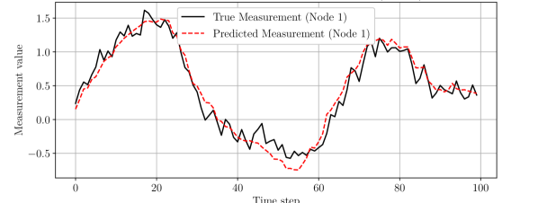
Figure 1 shows a representative 2D trajectory comparing the true state, the local node estimates, and the fused state estimate obtained using the NDKF. The NDKF’s fused estimate closely tracks the true state, while the EKF baseline deviates considerably, as indicated by the numerical RMSE in Table I, due to its mis‑specified measurement models. Figure 2 illustrates the measurement innovation residuals for Node 1. The low and stable residuals obtained with the NDKF, along with the numerical results reported in Table I, confirm its superior measurement update performance compared to the EKF baseline.
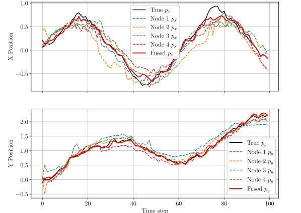
The experimental results show that in scenarios with significant nonlinearities and model mismatch, the proposed NDKF outperforms the distributed EKF baseline. By learning both the dynamics residual and the true measurement functions, the NDKF achieves much lower RMSE values (0.1209 for and 0.2642 for ) compared to the EKF (0.3964 and 0.4463, respectively), even though the EKF uses the correct measurement models for Nodes 3 and 4. While the EKF may perform well under near‑linear conditions, its reliance on fixed, mis‑specified analytical models leads to significant errors when facing true nonlinear behavior.
An implementation of NDKF, including the example provided in this section, is available in the GitHub repository accompanying this paper at:
https://github.com/sfarzan/NDKF
V Conclusion and Future Directions
We introduced the Neural-Enhanced Distributed Kalman Filter (NDKF), a data-driven framework that integrates learned neural network models within a consensus-based, distributed state estimation scheme. By replacing traditional process and measurement equations with learned functions and , NDKF is able to accommodate complex or poorly characterized dynamics while remaining robust in the presence of partial and heterogeneous observations. Our theoretical analysis identified key factors influencing filter convergence, including Lipschitz continuity of the neural approximations, proper noise covariance tuning, and adequate network connectivity for effective distributed fusion, along with a detailed computational complexity analysis. Experimental evaluations on a 2D system with multiple sensor nodes demonstrated the NDKF’s capability to reduce estimation error compared to a baseline distributed EKF, particularly under challenging nonlinear motion patterns.
Despite promising performance, several challenges remain. Future work may explore more advanced training and adaptive learning methods for nonstationary environments, alternative fusion strategies to improve scalability and fault tolerance, and extensions to the theoretical analysis–including robust estimation techniques to address adversarial noise distributions–to broaden the NDKF’s applicability.
References
- [1] R. Olfati-Saber, “Distributed kalman filter with embedded consensus filters,” in Proceedings of the 44th IEEE Conference on Decision and Control, 2005, pp. 8179–8184.
- [2] R. Olfati-Saber, J. A. Fax, and R. M. Murray, “Consensus and cooperation in networked multi-agent systems,” Proceedings of the IEEE, vol. 95, no. 1, pp. 215–233, 2007.
- [3] N. A. Carlson and M. P. Berarducci, “Federated kalman filter simulation results,” Navigation, vol. 41, no. 3, pp. 297–322, 1994.
- [4] R. Carli, A. Chiuso, L. Schenato, and S. Zampieri, “Distributed kalman filtering using consensus strategies,” in 2007 46th IEEE Conference on Decision and Control, 2007, pp. 5486–5491.
- [5] A. H. Jazwinski, Stochastic processes and filtering theory. Courier Corporation, 2007.
- [6] S. Julier and J. Uhlmann, “Unscented filtering and nonlinear estimation,” Proceedings of the IEEE, vol. 92, no. 3, pp. 401–422, 2004.
- [7] G. Battistelli and L. Chisci, “Stability of consensus extended kalman filter for distributed state estimation,” Automatica, vol. 68, pp. 169–178, 2016.
- [8] W. Li, G. Wei, F. Han, and Y. Liu, “Weighted average consensus-based unscented kalman filtering,” IEEE Transactions on Cybernetics, vol. 46, no. 2, pp. 558–567, 2016.
- [9] S. Julier and J. K. Uhlmann, “General decentralized data fusion with covariance intersection,” in Handbook of multisensor data fusion. CRC Press, 2017, pp. 339–364.
- [10] J. Hu, L. Xie, and C. Zhang, “Diffusion kalman filtering based on covariance intersection,” IEEE Transactions on Signal Processing, vol. 60, no. 2, pp. 891–902, 2012.
- [11] R. G. Krishnan, U. Shalit, and D. Sontag, “Deep kalman filters,” 2015. [Online]. Available: https://arxiv.org/abs/1511.05121
- [12] M. Fraccaro, S. r. K. Sø nderby, U. Paquet, and O. Winther, “Sequential neural models with stochastic layers,” in Advances in Neural Information Processing Systems, vol. 29, 2016.
- [13] G. Revach, N. Shlezinger, X. Ni, A. L. Escoriza, R. J. G. van Sloun, and Y. C. Eldar, “Kalmannet: Neural network aided kalman filtering for partially known dynamics,” IEEE Transactions on Signal Processing, vol. 70, pp. 1532–1547, 2022.
- [14] A. Krishnamoorthy and D. Menon, “Matrix inversion using cholesky decomposition,” in 2013 Signal Processing: Algorithms, Architectures, Arrangements, and Applications (SPA), 2013, pp. 70–72.