A Training-Free Length Extrapolation Approach for LLMs:
Greedy Attention Logit Interpolation (GALI)

Abstract

Transformer-based Large Language Models (LLMs) struggle to process inputs exceeding their training context window, with performance degrading due to positional out-of-distribution (O.O.D.) that disrupt attention computations. Existing solutions, fine-tuning and training-free methods, are limited by computational inefficiency, attention logit outliers or loss of local positional information. To address this, we propose Greedy Attention Logit Interpolation (GALI), a training-free length extrapolation method that maximizes the utilization of pretrained positional intervals while avoiding attention logit outliers through attention logit interpolation. The result demonstrates that GALI consistently outperforms state-of-the-art training-free methods. Our findings reveal that LLMs interpret positional intervals unevenly within their training context window, suggesting that extrapolating within a smaller positional interval range yields superior results—even for short-context tasks. GALI represents a significant step toward resolving the positional O.O.D. challenge, enabling more reliable long-text understanding in LLMs. Our implementation of GALI, along with the experiments from our paper, is open-sourced at https://github.com/AcademyCityL/GALI.

1 Introduction

Transformer-based Large Language Models (LLMs) have become indispensable for a wide range of natural language processing tasks, yet their performance is fundamentally constrained by the training context window, i.e., the maximum input length used during training. When tasked with processing input text that exceeds this predefined limit, LLMs exhibit sharp performance degradation, with perplexity (PPL) increasing exponentially as input length grows (Peng et al., 2023; Chen et al., 2023b; Xiao et al., 2023; Han et al., 2024; Jin et al., 2024; An et al., 2024b). This limitation poses significant challenges for applications requiring robust long-text understanding, such as document summarization, legal text analysis, and conversational AI.

The core issue lies in the model’s inability to generalize beyond the positional distributions encountered during pretraining, leading to disruptions in attention score computations—a phenomenon known as positional out-of-distribution (O.O.D.) (Chen et al., 2023b; Jin et al., 2024; Xu et al., 2024). Addressing positional O.O.D. is critical for enhancing LLMs’ length extrapolation capabilities and enabling reliable long-text processing.

Existing approaches to mitigating positional O.O.D. can be classified into three categories: (1) Lambda-Shaped Attention Mechanisms, which stabilize PPL but compromise the ability to capture long-range dependencies across distant tokens (Xiao et al., 2023; Han et al., 2024; Jiang et al., 2024; Li et al., 2024a; Zhang et al., 2024); (2) Fine-Tuning on long texts, which involves training on datasets with extended positional contexts using interpolation (Chen et al., 2023b, a; Xiong et al., 2023; Li et al., 2023; Ding et al., 2024; Li et al., 2024b; Wu et al., 2024) or extrapolation (Zhu et al., 2023; Chen et al., 2023c; Ding et al., 2024). While effective, this approach is resource-intensive and still encounters cases where positional IDs exceed its fine-tuned context window; and (3) Training-free length extrapolation methods, which include Rotary Position Embedding (RoPE) frequency interpolation techniques (e.g., Neural Tangent Kernel (NTK), Dyn-NTK, YaRN) (LocalLLaMA, 2023b, a; Peng et al., 2023) and inputs rearrangement strategies (e.g., SelfExtend, ChunkLlama) (Jin et al., 2024; An et al., 2024b). They partially mitigate positional O.O.D. but suffer from limitations, such as the emergence of attention logit outliers or the loss of local positional information.

To overcome the challenges above, this paper introduces Greedy Attention Logit Interpolation (GALI), a novel training-free length extrapolation method tailored for transformer-based LLMs. GALI has two primary objectives: (1) to maximize the utilization of pretrained positional intervals, thereby minimizing disruption to attention computations, and (2) to mitigate outliers in attention logits through an attention logit interpolation strategy.

Key Innovations in GALI: First, GALI optimizes the utilization of pretrained position intervals. During the prefill phase, the method retains the model’s native position IDs for tokens within the training context window, ensuring that the corresponding hidden states maintain the quality achievable by the original model. GALI assigns interpolated position IDs chunk-wise for tokens exceeding the training context window, balancing efficiency with quality. During the decode phase, GALI dynamically generates interpolated position IDs for newly generated tokens, minimizing interpolation-induced disruptions during token generation. Second, GALI introduces a novel approach to compute attention logits for interpolated positional intervals. With the help of linear interpolated position IDs, GALI performs local linear interpolation directly on attention logits instead of computing positional embeddings, avoiding the outlier issues commonly associated with positional O.O.D. Furthermore, it simulates the oscillatory characteristics of RoPE, by adding Gaussian noise proportional to relative distances, enhancing the model’s positional sensitivity.

GALI offers a training-free, plug-and-play solution that operates exclusively during inference by maximizing the utilization of pretrained positional intervals and focusing on attention logit interpolation. It extends the usable context window of LLMs, significantly improving long-text processing capabilities while integrating seamlessly with existing long-context frameworks.

Empirical Evaluation: We evaluated GALI across three benchmarks, alongside a quantitative analysis of attention distribution, covering both real-world long-context applications and long-context language modeling. The results demonstrate that GALI consistently outperforms state-of-the-art training-free methods, achieving superior performance across diverse long-context scenarios. Furthermore, our analysis reveals a performance-enhancing strategy based on inconsistencies in how models interpret positional intervals. Notably, applying extrapolation methods within a smaller range of positional intervals leads to better results, even for short-context tasks. In summary, GALI represents a significant advancement in addressing the positional out-of-distribution (O.O.D.) challenge, unlocking new potential for LLMs in long-text understanding and processing.

Our main contributions are summarized as follows:

• A Novel Training-Free Length Extrapolation Method: We introduce Greedy Attention Logit Interpolation (GALI), a training-free method that maximizes the utilization of pretrained positional intervals while leveraging attention logit interpolation to mitigate outliers, effectively addressing the positional O.O.D. problem in long-text processing for LLMs.

• Comprehensive Evaluation and Analysis: We conducted a comprehensive comparison and analysis of GALI and other state-of-the-art training-free length extrapolation methods. While demonstrating GALI’s superior performance, we also identified a more effective length extrapolation strategy.

2 Background

Rotary Position Embedding (RoPE): RoPE (Su et al., 2024) is a technique that encodes positional information by applying rotary transformations to token embeddings, enabling relative position modeling in transformers. Given two token embeddings $\bm{x}_{m},\bm{x}_{n}\in\mathbb{R}^{l}$ as query and key corresponding to position $m$ and $n$, the projection matrix $\bm{W}_{Q},\bm{W}_{K}\in\mathbb{R}^{d\times l}$, RoPE applies a rotation to the projected token embeddings, i.e., $\bm{q}_{m}^{r}=(\bm{W}_{Q}\bm{x}_{m})e^{im\bm{\theta}}$, $\bm{k}_{n}^{r}=(\bm{W}_{K}\bm{x}_{n})e^{in\bm{\theta}}$, where $\bm{\theta}=[b^{0},b^{-2/d},\dots,b^{-2(j-1)/d}]$, $j\in[1,2,\dots,d/2]$ and $b$ is originally set to 10000. After that, the inner product between the query $\bm{q}_{m}^{r}$ and key $\bm{k}_{n}^{r}$ can be represented by the real part of ${\bm{q}_{m}^{r}}^{*}\bm{k}_{n}^{r}$, i.e.:

$$\langle\bm{q}_{m}^{r},\bm{k}_{n}^{r}\rangle_{\mathbb{R}}=\operatorname{Re}(\langle(\bm{W}_{Q}\bm{x}_{m})e^{im\bm{\theta}},(\bm{W}_{K}\bm{x}_{m})e^{in\bm{\theta}}\rangle_{\mathbb{C}})$$

$$=\operatorname{Re}\left[\sum_{j=0}^{d/2-1}({\bm{W}_{Q}\bm{x}_{m}})_{[2j:2j+1]}(\bm{W}_{K}\bm{x}_{n})^{*}_{[2j:2j+1]}e^{i(m-n)\theta_{j}}\right]$$

$$=a(\bm{x}_{m},\bm{x}_{n},m-n)$$ (1)

$g(\cdot)$ is the function mapping token embeddings $\bm{x}_{m},\bm{x}_{n}$ to the attention logit, which depends on their relative distance and is irrelevant to their absolute positions. Additionally, RoPE exhibits a long-term decay as relative distance increases (Su et al., 2024), as illustrated in Figure 1. Our proposed method, GALI, leverages two key properties of RoPE to achieve position interpolation and length extrapolation effectively.

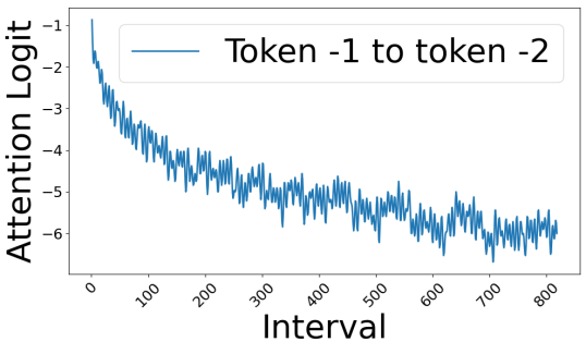
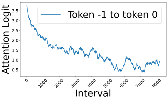
Figure 1: Visualization of long-term decay in attention logits. The sentence “The quick brown fox jumps over the lazy dog.” is fed into a one-layer Llama3-8b-ins model. Figure 1 shows the attention logits from the last token to the second-to-last token. Figure 1 presents the logits from the last token to the first token. As the positional ID interval increases from 1 to 819, a clear decay phenomenon in the logits is observed.

Positional Out-Of-Distribution (O.O.D.): In Transformer architectures, the self-attention mechanism is inherently position-agnostic, necessitating the use of position embeddings to encode positional information for processing ordered inputs (Dufter et al., 2021; Kazemnejad et al., 2024). Even in large language models (LLMs) with causal attention, explicit positional encoding through position embeddings remains the standard approach. During inference, when LLMs encounter input sequences exceeding the maximum length seen during training, the use of unseen position IDs causes a positional out-of-distribution (O.O.D.) issue, leading to degraded performance (Chen et al., 2023b; Jin et al., 2024; Xu et al., 2024). In the Rotary Position Embedding (RoPE) mechanism, extrapolating position IDs beyond the training range introduces untrained positional intervals, disrupting the attention score distribution (Chen et al., 2023b). In contrast, position interpolation has yielded more stable attention distributions, requiring fewer fine-tuning steps (Chen et al., 2023b). This observation has inspired subsequent interpolation-based methods (Chen et al., 2023b, a; Xiong et al., 2023; Li et al., 2023; Ding et al., 2024; Li et al., 2024b; Wu et al., 2024), as well as training-free approaches that map position interpolation into alternative frequency dimensions in embeddings (LocalLLaMA, 2023b, a; Peng et al., 2023). Recent work has explored other training-free length extrapolation techniques, such as group position IDs (Jin et al., 2024) or chunk attention (An et al., 2024b).

3 Method

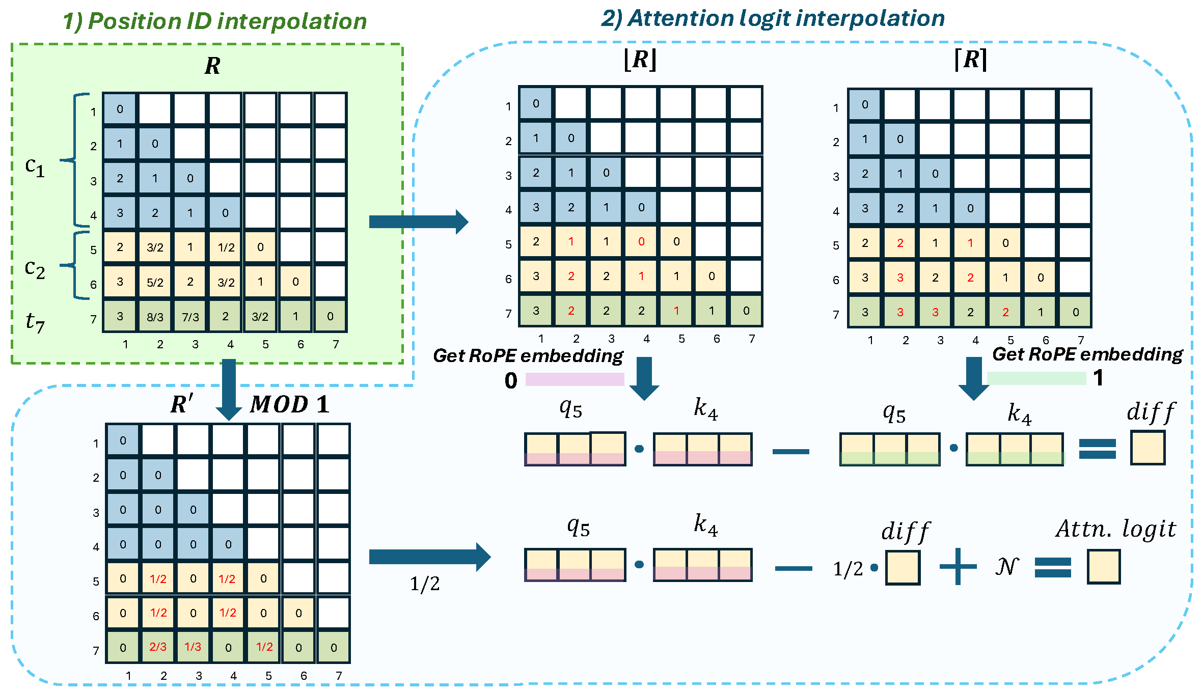
Figure 2: The overall procedure of the proposed GALI framework. The green dashed line illustrates position ID interpolation, while the blue dashed line shows attention logit interpolation. In this example, the training context window $L_{tr}$ is 4, the chunk size $s$ is 2, the local window $L_{w}$ is 2, and the prefill length is 6. Chunks are denoted as $c_{1}$ (first chunk) and $c_{2}$ (second chunk), while $t_{7}$ represents the first generated token. The relative distance matrix $R$ incorporates $\lceil R\rceil$, $\lfloor R\rfloor$, and $R^{\prime}$, representing ceiling, floor, and modulo operations, respectively. Red numbers in the relative distance matrix indicate interpolated positional intervals and $\mathcal{N}$ represents the Gaussian noise.

This section presents Greedy Attention Logit Interpolation (GALI), a novel training-free position interpolation method designed to enhance the utilization of pretrained positional information while ensuring stable attention computations. GALI is guided by two objectives: (1) Maximizing the use of pretrained positional information, i.e., the positional intervals encountered during pre-training. To do so, we perform minimal-impact position interpolation for each chunk in the prefill phase and newly generated tokens during the decoding phase. (2) Preventing outliers in attention logits by avoiding direct computation of position embeddings for interpolated positions. We apply local linear interpolation to the attention logits based on interpolated position IDs and simulate RoPE’s oscillatory behavior by introducing Gaussian noise. The process is shown in Figure 2.

3.1 Position ID Interpolation

The proposed GALI introduces a strategy for position ID interpolation to handle inputs exceeding the maximum training length, aiming to fully utilize pretrained relative positional intervals. During the prefill phase, GALI segments the input portion beyond the maximum training length into multiple chunks and performs position ID interpolation for each chunk individually. In contrast, the portion within the maximum training length remains unchanged, without any interpolation. This approach provides several advantages. First, if the input length does not exceed the maximum training length, the prefill phase remains entirely unaffected, preserving the model’s original capabilities. Second, when the input length surpasses the maximum training length, the text within the training range can fully leverage the pretrained relative positional intervals to generate hidden states based on the model’s original performance. Finally, for inputs beyond the training length, GALI can apply position ID interpolation in a manner that minimizes the impact on model quality for each chunk. Specifically, each chunk only adds the exact number of new position IDs it requires. This ensures the interpolation process maintains a balance between computational efficiency and fidelity.

This approach draws inspiration from Dyn-NTK(LocalLLaMA, 2023a), which adjusts scaling factors to handle inputs of varying lengths. However, dynamic NTK applies a uniform interpolation across the entire input during the prefill phase, potentially overlooking the varying interpolation requirements of individual tokens. For instance, a token just beyond the training context window only requires the interpolation of one new position ID, whereas subsequent tokens would require progressively more. Ideally, the interpolation for each token would be customized to minimize its impact on quality. However, performing interpolation at the token level is computationally inefficient. To address these challenges, GALI segments the input exceeding the training length into chunks and applies interpolation only for the position IDs that extend beyond the training range within each chunk. By tailoring interpolation to the specific needs of each chunk, GALI avoids the uniform scaling factors used in previous methods, such as NTK, Dyn-NTK, YaRN, or SE, which can lead to suboptimal results. This chunk-wise strategy ensures a more adaptive and efficient interpolation process while maintaining model performance.

Building on insights from prior studies, GALI retains a local window of size $L_{w}$ around the current token to preserve the original positional intervals within this range. This design allows the current token to effectively interpret its immediate context using the model’s pretrained capabilities. During the decode phase, where tokens are generated sequentially, GALI dynamically interpolates the required position IDs for each newly generated token, focusing on minimizing quality degradation. Specifically, in the prefill stage, given an input sequence $S=(w_{1},w_{2},\dots,w_{L_{tr}},\dots,w_{L})$ where $L_{tr}$ is the size of training context window and $L$ is the input length in the prefill stage. We first divide it into chunks $C=(c_{1},c_{2},\dots,c_{L_{c}})$, where the size of $c_{1}$ is $L_{tr}$ and other chunks have a size $s$, so the $L_{c}=\lceil{\frac{L-L_{tr}}{s}}\rceil$. After that, we assign position IDs $S=(s_{1},s_{2},\dots,s_{L_{c}})$ for each chunk, where $s_{1}=[0,1,\dots,L_{tr}-1]$ and others are interpolated position IDs according to the following formula:

$$\begin{cases}&j>1;\\ &{g}_{j}=\lceil{\frac{\sum_{i=1}^{j}{len(c_{i})}-L_{w}}{L_{tr}-L_{w}}}\rceil;\\ &{v}_{j}=1/{g}_{j};\\ &s_{j}=[0,1*{v}_{j},2*{v}_{j},\dots,({g}_{j}-1)*{v}_{j},1,\dots,\\ &L_{tr}-L_{w}-1,L_{tr}-L_{w},\dots,L_{tr}-1]\end{cases}$$ (2)

We first calculate the minimal group size ${g}_{j}$ required for each chunk after excluding the local window $L_{w}$ and then apply linear interpolation within each group. During the decode phase, each newly generated token is treated as an individual chunk of size 1, enabling the computation of minimally impactful interpolated position IDs.

3.2 Attention Logit Interpolation

When calculating attention scores, we approximate attention logits for interpolated positions using local linear interpolation based on interpolated position IDs, while introducing Gaussian noise that scales with relative position intervals. Unlike NTK or YaRN, our methods avoid outlier attention logits from the position embeddings (Chen et al., 2023b). RoPE’s trigonometric functions, while effective within pretrained relative position intervals, can produce extreme values during interpolation, leading to abnormal attention logits. To mitigate this, we bypass position embeddings and directly approximate attention logits. Building on the monotonic trends and oscillatory behavior observed in RoPE, as shown in Figure 1, we hypothesize that for two tokens with an interpolated relative distance (e.g., $7.r$), their attention logits—excluding oscillatory effects—should lie between $g(7)$ and $g(8)$, with their exact value determined by $r$. To achieve this, we compute attention logits for each QK pair with interpolated relative position intervals using local linear interpolation and simulate oscillatory behavior by adding Gaussian noise, whose variance increases with relative position intervals. This method eliminates the outliers identified in the PI study and produces interpolated attention logits for new relative position intervals in a training-free and effective manner.

Specifically, given two token embeddings $\bm{x}_{m},\bm{x}_{n}\in\mathbb{R}^{l}$ as query and key corresponding to position $m$ and $n$. Note here the $m$ and $n$ can be interpolated float position ids. Let $r=m-n$, when ${r}{\%}1=0$ we compute their attention logits directly which means their relative position interval was pretrained. For the case ${r}{\%}1>0$, which means that their relative positional interval is interpolated, we then compute the attention logit $a(\bm{x}_{m},\bm{x}_{n},r)$ using the formula:

$$a(\bm{x}_{m},\bm{x}_{n},r)=a(\bm{x}_{m},\bm{x}_{n},\lfloor{r}\rfloor)-[a(\bm{x}_{m},\bm{x}_{n},\lfloor{r}\rfloor))-$$ (3)

$$a(\bm{x}_{m},\bm{x}_{n},\lceil{r}\rceil]*({r}{\%}1)+\mathcal{N}(0,{\frac{r}{L_{tr}}}^{2})$$

Where $\%$ represents the $\mod$ operation. To enable matrix modification of relative distances during computation, we adopted an approximate implementation that replaces $r$ with $r=\lceil{m}\rceil-n$, as detailed in the pseudo-code (Appendix A).

4 Experiments

We evaluate GALI on Llama3-8B-ins models across two task categories: real-world long-context tasks and long-context language modeling tasks. For comparison, we implement all published training-free length extrapolation methods, including NTK(LocalLLaMA, 2023b), Dyn-NTK(LocalLLaMA, 2023a), YARN(Peng et al., 2023), SelfExtend(Jin et al., 2024), and ChunkLlama(An et al., 2024b). The following sections describe the experimental setup for each task. Appendix B details data statistics.

4.1 Emperiments Setup

Real-world long-context task: We evaluate GALI on two widely used long-context benchmarks, LongBench(Bai et al., 2024) and L-Eval(An et al., 2024a). LongBench is a bilingual long-context understanding benchmark with 21 datasets crossing 6 tasks, including Single-Document QA, Multi-Document QA, Summarization, Few-shot Learning, Synthetic Task, and Code Completion. We use 16 English datasets from LongBench. L-Eval is a comprehensive long-context evaluation suite with 20 sub-tasks, 508 long documents, and over 2000 human-labeled query-response pairs. It consists of closed-ended and open-ended task groups. We focus on closed-ended groups, which assess reasoning and understanding over a long-context. For consistency, we follow the official task prompt templates and truncation strategies from the respective benchmarks.

Long-context language modeling task: To evaluate GALI’s long-context language modeling capabilities, we use PG19(Rae et al., 2019), an open-vocabulary language modeling benchmark derived from Project Gutenberg. PG19 consists of over 28,000 books published before 1919, covering diverse genres and writing styles. We use its test split, which includes 100 samples.

	Methods	Single document QA			Multi document QA			Summarization			Few-shot Learning			Synthetic		Code		Average
		NarrativeQA	Qasper	MultiField-en	HotpotQA	2WikiMQA	Musique	GovReport	QMSum	MultiNews	TREC	TriviaQA	SAMSum	PassageCount	PassageRe	Lcc	RepoBench-P
Llama3-8b-ins-4k	Original	17.83	40.62	47.02	40.97	35.15	20.99	27.76	19.70	24.62	71.00	89.54	42.31	6.00	23.50	56.96	49.06	38.31
	SelfExtend-16k	23.34	44.59	51.22	44.91	37.43	29.50	28.52	22.14	24.34	75.50	90.71	42.58	7.50	92.50	54.99	50.83	45.04
	ChunkLlama-16k	20.91	40.15	49.87	47.71	40.80	28.75	30.37	21.81	24.32	74.50	90.29	41.78	2.50	56.75	58.99	57.55	42.94
	NTK-16k	22.59	46.25	53.21	51.91	37.51	26.56	30.69	22.74	24.03	73.50	90.46	42.20	11.50	73.00	34.53	36.39	42.32
	Dyn-NTK-16k	18.65	44.91	51.37	46.28	37.57	28.03	30.20	21.53	24.48	76.00	89.11	42.88	9.00	74.50	53.91	32.65	42.57
	YaRN-16k	16.43	40.13	53.04	45.93	33.66	28.51	30.40	22.42	23.24	75.50	91.04	44.53	6.50	86.50	43.26	48.26	43.08
	(Ours)GALI-16k	24.69	45.26	51.78	51.33	37.16	30.79	29.28	22.65	24.63	77.00	91.61	42.92	9.00	95.5	56.84	49.04	46.22
Llama3-8b-ins-8k	Original*	21.71	44.24	44.54	46.82	36.42	21.49	30.03	22.67	27.79	74.50	90.23	42.53	0.00	67.00	57.00	51.22	42.39
	SelfExtend-16k*	21.50	43.96	50.26	48.18	28.18	25.58	34.88	23.83	26.96	75.50	88.26	42.01	4.12	88.00	36.58	37.73	42.22
	ChunkLlama-16k	23.87	43.86	46.97	49.37	35.34	26.52	31.06	21.99	24.45	76.00	90.73	42.29	7.00	72.00	59.93	56.98	44.27
	NTK-16k	8.04	43.85	47.94	20.44	34.32	1.57	24.31	13.22	24.12	74.50	52.18	33.12	4.50	45.50	46.84	38.71	32.07
	Dyn-NTK-16k	8.19	43.31	47.91	34.63	35.26	7.92	26.83	17.85	24.51	76.50	71.72	39.15	5.67	83.50	56.58	46.39	39.12
	YaRN-16k	12.39	42.60	51.70	40.06	35.03	12.81	30.30	22.56	23.51	75.50	82.99	42.31	6.50	89.00	50.51	51.58	41.83
	(Ours)GALI-16k	25.88	45.65	47.09	51.07	37.42	28.75	30.09	22.7	24.58	77.00	90.91	42.43	6.00	83.00	57.04	53.06	45.17
Llama3-8b-ins-8k	Original*	21.71	44.24	44.54	46.82	36.42	21.49	30.03	22.67	27.79	74.50	90.23	42.53	0.00	67.00	57.00	51.22	42.39
	SelfExtend-32k*	12.04	12.10	20.15	8.22	9.68	3.89	27.90	14.58	22.13	61.00	82.82	1.40	2.37	2.83	57.87	56.42	24.71
	SelfExtend-32k	26.27	44.23	50.19	48.28	38.29	29.19	29.24	22.68	24.59	76.00	90.16	42.45	8.00	88.00	57.47	49.51	45.28
	ChunkLlama-32k	24.48	42.37	47.05	48.79	34.53	26.94	32.08	23.40	24.36	76.00	90.46	42.08	6.50	72.00	59.52	60.54	44.44
	NTK-32k	7.31	45.11	53.18	52.31	37.70	27.37	29.37	21.45	23.69	73.50	78.25	41.83	9.00	69.00	34.25	36.12	39.97
	Dyn-NTK-32k	23.06	43.95	48.55	52.68	37.46	25.22	31.53	22.19	24.52	77.00	90.96	42.42	8.00	71.50	56.77	43.78	43.72
	YaRN-32k	17.09	40.90	52.51	46.40	33.92	29.47	29.93	22.69	23.11	75.00	91.29	42.54	5.50	89.50	46.50	51.38	43.61
	(Ours)GALI-32k	28.63	45.66	47.23	51.07	38.35	29.00	29.98	22.79	24.59	77.00	91.13	42.38	5.50	83.00	57.07	52.63	45.38

Table 1: Performance comparison across different backbone LLMs and training-free length extrapolation methods. The best result in each experiment is bolded. Results marked with ^* are reported by LongBench (Jin et al., 2024). The number following each method denotes the target context window size (e.g., 16k represents 16 × 1024 tokens). ”Original” refers to evaluations conducted using the backbone model in the left column. Additional results using the Llama2-7B-Chat-4K backbone are provided in Appendix D.1.

Backbone models and baseline methods: We use Llama3-8b-ins-4k (Llama3-4k) and Llama3-8b-ins-8k (Llama3-8k) as backbone models, where the number following each model indicates its initial context window size. We obtain Llama3-4k backbone via modifying its max_position_embedding parameter. We use shorter-versions of Llama3-8b-ins over other LLMs with shorter training context windows like LLama2 since it cannot fully understand all pretrained positional intervals, which limits GALI’s effectiveness in practice. The effective understanding range of LLMs is shorter than their maximum training window, as evidenced in (Jin et al., 2024; Hsieh et al., 2024). For the baseline methods, we compare with NTK(LocalLLaMA, 2023b), Dyn-NTK(LocalLLaMA, 2023a), YaRN(Peng et al., 2023) using huggingface implementation and SelfExtend(Jin et al., 2024), ChunkLlama(An et al., 2024b) with their official implementation. They are all of the training-free length extrapolation methods up to now. The implementation details of these methods can be found in Appendix C.

4.2 Real-World long-context Task Results

The LongBench results (Table 1) highlight GALI’s strong average performance on the Llama3-8b-ins backbone series, surpassing both the 4k and 8k backbone models and other methods. GALI excels in question answering (QA) and few-shot learning tasks but showed weaker performance in summarization, synthetic, and code-related tasks. While extending the context window to 32k improves performance on Llama3-8k compared to 16k, it remains less effective than using 16k on Llama3-4k. This consistent trend in Figure 3(a) highlights limitations in extrapolation performance, which we analyze below.

Firstly, LLMs interpret positional intervals differently within their training context window, as noted in (Hsieh et al., 2024). This explains why using a 16k context window on Llama3-4k outperformed using the same window on Llama3-8k. Since LLMs are trained via next-token prediction, smaller positional intervals are more trained and thus better understood. The difference between models lies in the range of positional intervals they can fully comprehend based on their training context window. As a result, all methods except ChunkLlama perform better with a 16k context window on the Llama3-4k than with the same context window on the Llama3-8k. Secondly, despite all methods aiming for training-free length extrapolation, they employ fundamentally different approaches. GALI, NTK, Dyn-NTK, and YaRN focus on generalizing positional intervals, creating smaller but more usable intervals from pretrained ones. Among these, GALI generates only the minimal number of new intervals required, maximizing the reliance on pretrained intervals. Other methods predefine a target context window and fix the number and size of new intervals. Dyn-NTK only decides whether to generate new intervals based on input length without minimizing their quantity. SE and ChunkLlama do not create new positional intervals but instead redistribute inputs within existing intervals through input rearrangement. This leads to differences in practice: GALI maps inputs to the full range of the positional intervals of the training context window, while NTK, Dyn-NTK, YaRN and SelfExtend map inputs to predefined positional interval ranges based on the target context window (e.g. in SelfExtend, a larger context window leads to a larger group size). ChunkLlama determines interval ranges via hyperparameters such as chunk size and local window. The performance gap when using 16k and 32k context windows on Llama3-8k reflects these differences. Figure 6(b) shows that most LongBench dataset lengths are below 16k when using the Llama3 tokenizer. However, NTK, Dyn-NTK, YaRN and SelfExtend still benefit significantly from expanding to 32k, particularly on HotpotQA and Musique. This is because most of the data in HotpotQA and Musique is concentrated below 16k. A 32k context window can map them to the positional interval range [0–4096), while a 16k one maps them to the range [0–8192) (For SelfExtend, this range is not fixed and depends on the specific local window and group size. However, it typically falls within a smaller positional interval range.). In contrast, GALI’s results for data shorter than 16k remain nearly unchanged, while ChunkLlama exhibits slight fluctuations. Overall, these methods that do not rely on predefined target context windows show limited improvement since most dataset lengths remain below 16K. However, on NarrativeQA—the longest dataset—GALI shows a substantial improvement from 25.88 to 28.63, outperforming all other methods.

	Methods	Coursera	GSM	QuALITY	TOFEL	SFiction	CodeU	Average
Llama3-8b-ins-4k	Original	53.34	75.00	59.41	81.41	60.94	4.44	55.76
	SelfExtend-16k	55.23	79.00	64.36	79.18	67.97	5.56	58.55
	ChunkLlama-16k	52.62	77.00	63.37	81.04	60.16	3.33	56.25
	NTK-16k	57.70	80.00	63.86	81.04	64.06	5.56	58.70
	Dyn-NTK-16k	54.07	75.00	64.36	82.16	67.97	1.11	57.44
	YaRN-16k	56.40	81.00	59.40	79.18	64.06	5.56	57.6
	(Ours)GALI-16k	56.54	74.00	65.35	84.06	66.41	8.89	59.21
Llama3-8b-ins-8k	Original	53.05	-	-	-	60.16	4.44	39.22
	SelfExtend-16k	55.38	-	-	-	64.06	5.56	41.67
	ChunkLlama-16k	53.34	-	-	-	61.72	5.56	40.21
	NTK-16k	52.03	-	-	-	42.97	0.00	31.67
	Dyn-NTK-16k	52.03	-	-	-	52.34	2.22	35.53
	YaRN-16k	55.96	-	-	-	62.5	5.56	41.34
	(Ours)GALI-16k	54.65	-	-	-	65.63	6.67	42.32
Llama3-8b-ins-4k	Original	53.34	75.00	59.41	81.41	60.94	4.44	55.76
	SelfExtend-32k	54.51	80.00	64.36	77.70	67.97	5.56	58.35
	ChunkLlama-32k	53.20	75.00	63.37	81.04	63.28	2.22	56.35
	NTK-32k	52.91	82.00	61.39	79.93	67.19	2.22	57.6
	Dyn-NTK-32k	52.33	76.00	63.86	82.16	71.88	3.33	58.26
	YaRN-32k	53.05	73.00	59.41	79.55	68.75	5.56	56.55
	(Ours)GALI-32k	54.17	74.00	65.35	84.06	68.75	7.78	59.10
Llama3-8b-ins-8k	Original	53.05	-	-	-	60.16	4.44	39.22
	SelfExtend-32k	53.92	-	-	-	65.63	3.33	40.96
	ChunkLlama-32k	54.36	-	-	-	64.06	5.56	41.33
	NTK-32k	58.28	-	-	-	59.38	1.11	39.59
	Dyn-NTK-32k	54.36	-	-	-	64.06	6.67	41.70
	YaRN-32k	55.23	-	-	-	67.19	7.78	43.40
	(Ours)GALI-32k	54.17	-	-	-	66.41	7.78	42.79

Table 2: Performance comparison across different backbone LLMs and training-free length extrapolation methods. The best result in each experiment is bolded. The GSM, QuALITY, and TOEFL were excluded from this comparison because their sequence lengths remain below 8192 tokens when using the Llama3 tokenizer, making them unsuitable for long-context evaluation. Results for these three datasets, along with those for all datasets using the Llama2-7B-Chat-4K (Llama2-4k) backbone, are provided in Appendix D.1.

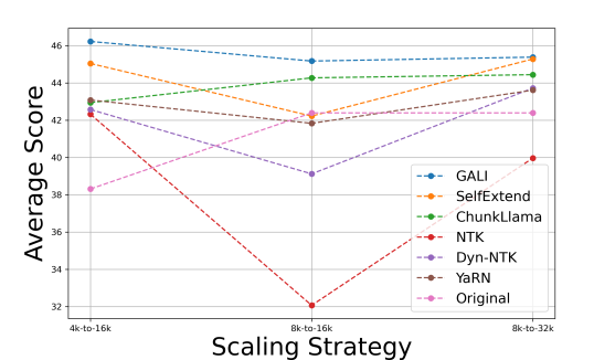
(a) LongBench

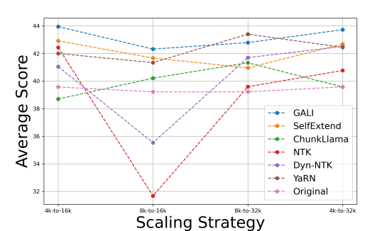
(b) L-Eval

Figure 3: The trend of average scores across different methods and settings. The X-axis tick “4k-to-16k” represents an initial context window of 4k and a target window of 16k. For a more meaningful comparison, the average scores are computed on the three long-text datasets in L-Eval: Coursera, SFiction, and CodeU.

The L-Eval results further support our analysis. As shown in Table 2, GALI achieved the highest average performance, except when using a 32k context window on the Llama3-8k. Consistent with LongBench, where 32k on Llama3-8k performed slightly better than 16k but remained inferior to 16k on Llama3-4k, aligning with our previous observations. Since Llama3 better understands closer positional intervals, other methods benefit from mapping text to a smaller range of positional intervals, giving GALI a relative disadvantage at 32k on Llama3-8k. However, GALI still achieved the second-best performance. To investigate further, we tested GALI with a 32k context window on Llama3-4k, forcing it to operate exclusively within the [0, 4096) range of positional intervals. Under these conditions, GALI once again achieved the best results. Figure 3(b) shows the overall performance trends. Additionally, it is worth noting that when using the Llama3 tokenizer, GSM, QuALITY, and TOEFL lengths are all below 8192, where SE, YaRN, and NTK outperform the backbone models as shown in Appendix D.1, further validating our findings.

Experiments on LongBench and L-Eval show that training-free length extrapolation methods benefit from mapping text to smaller relative positional intervals, compensating for models’ uneven positional understanding. GALI, however, minimizes new intervals while utilizing the full range of pretrained intervals, which can be disadvantageous in some cases. As models improve, GALI’s direct attention logit estimation enhances context comprehension, delivering superior stability without requiring hyperparameter tuning.

	Methods	1k	4k	8k	12k	16k	20k	24k	28k	32k
Llama3-8b-ins-8k	SelfExtend	11.52	11.54	11.32	11.18	11.07	10.97	11.01	11.04	10.91
	ChunkLlama	11.72	11.77	11.54	11.39	11.27	-	-	-	-
	NTK	11.93	11.94	11.67	11.50	11.39	13.03	23.00	42.95	77.41
	Dyn-NTK	11.51	11.53	12.75	66.88	166.86	269.93	334.83	360.57	365.36
	YaRN	11.93	11.81	11.48	11.30	11.18	11.06	11.10	11.13	11.18
	(Ours)GALI	11.52	11.54	11.35	11.25	11.17	11.09	11.14	11.18	11.05

Table 3: Performance of Diverse Models on the PG19 Dataset Across Varying Context Window Sizes.

4.3 Long Language Modeling Task Results

The language modeling results are shown in Table 3. Due to OOM, we cannot get ChunkLlama’s PPL results when setting the maximum position embedding to 32768. Except for NTK and DYN-NTK, all methods maintained a stable PPL without exploding. While low PPL does not guarantee better real-world task performance, an exploding PPL is a clear indicator of performance degradation in downstream tasks. Notably, GALI achieved the second-lowest PPL, demonstrating superior stability in length extrapolation. We tested PPL using a 16k contest window with Llama2-4k backbone. Please refer to the Appendix D.2.

(a) Attention Score Matrix Differences

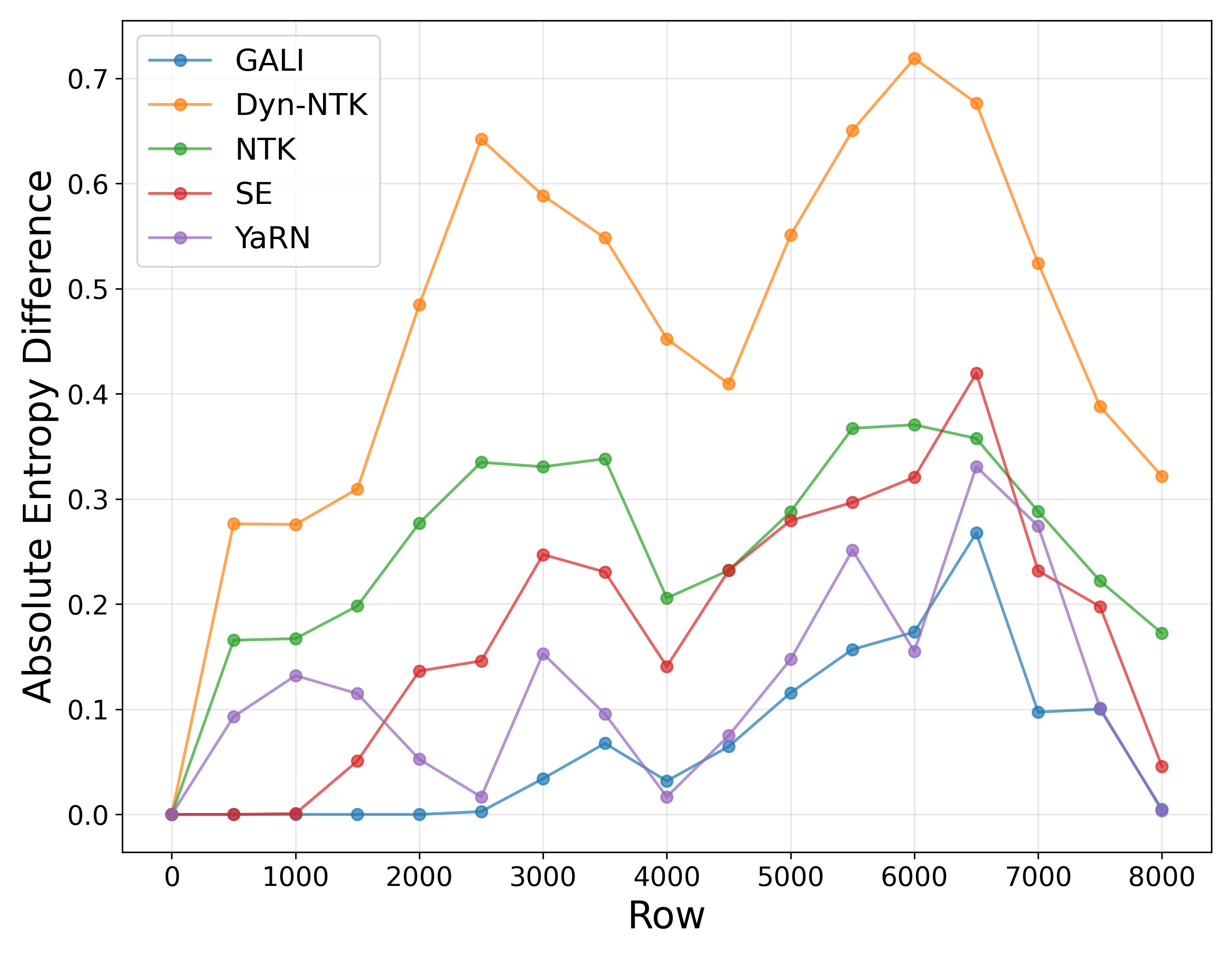
(b) Row Entropy Differences (2K)

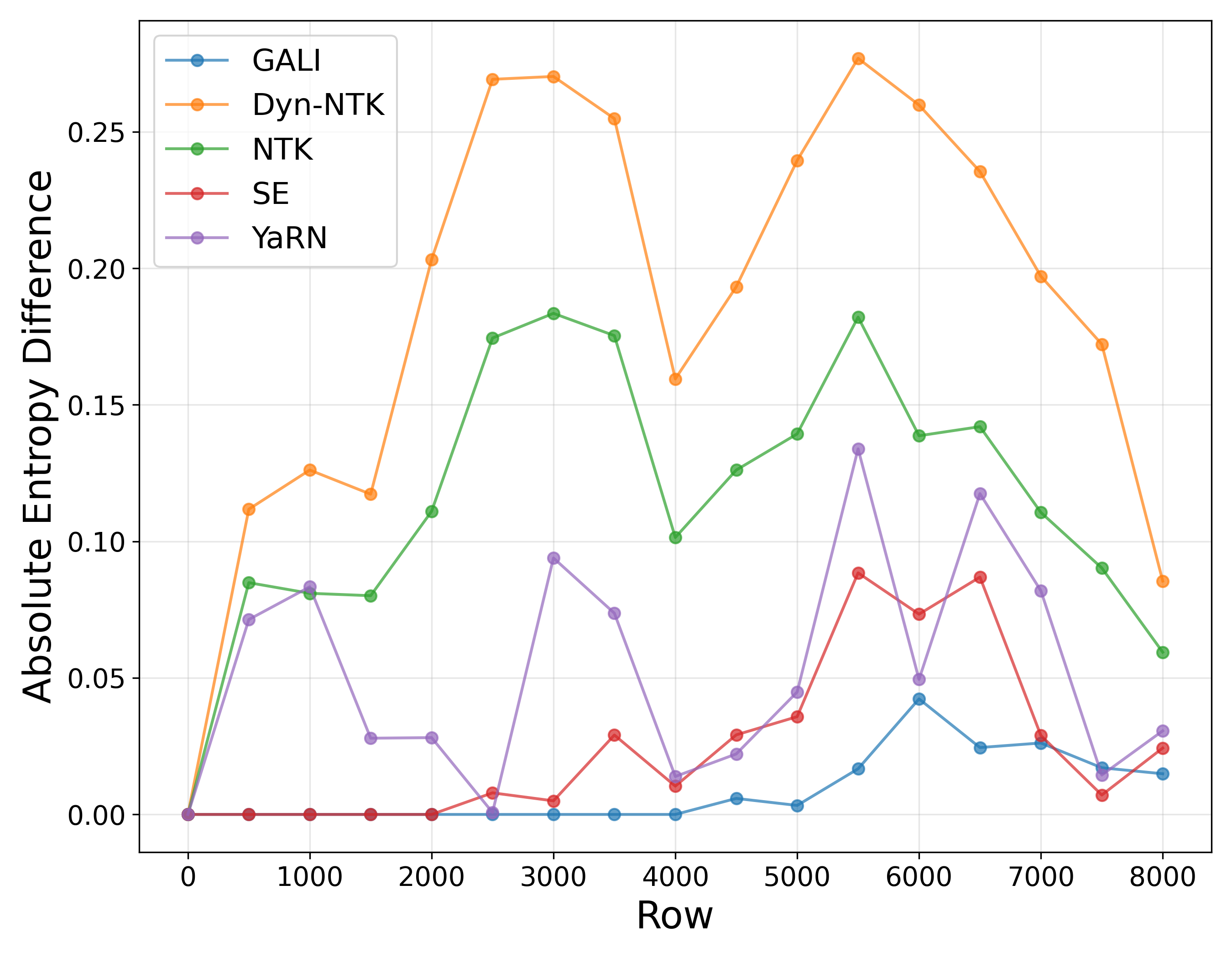
(c) Row Entropy Differences (4K)

Figure 4: Differences in attention score metrics and row-wise entropy across methods compared to the original LLM. (a) represents the attention score matrix differences. The values show the sum of the absolute differences between the attention scores of the length interpolation methods and the model trained on its training context window. (b) and (c) show row-wise entropy differences. 2K indicates methods using [0, 2048) positional intervals, while 4k shows the methods using positional intervals within [0, 4096). The figures are generated using a sample from NarrativeQA with a prefill length of 8091 tokens. More details on the attention score distributions can be found in Appendix D.3.

4.4 Attention Distribution Analysis

As discussed in Section 4.2, the effectiveness of training-free length extrapolation methods is influenced not only by the algorithm itself but also by the model’s understanding of positional intervals within its training context window. We propose a new comparison approach to fairly compare different length extrapolation methods while eliminating the positional interval understanding bias inherent to the model. Instead of applying extrapolation methods across a full context window, we first restrict them to a smaller positional interval range. We then extend this range to match the model’s training context window and compare the resulting attention distribution against the model’s original attention distribution. In this scenario, the closer the extrapolated attention distribution is to the model’s original attention distribution, the more effectively the extrapolation method performs within a smaller positional interval range, indicating that it aligns more closely with the model’s inherent understanding. Consequently, as the model’s understanding improves, the performance of the length extrapolation method will also improve. More concretely, we applied these training-free length extrapolation methods to Llama3-8b-ins-2k (Llama3-2k) and Llama3-4k backbones, and compared the resulting attention score distribution with Llama3-8k. The results, shown in Figure 4(a), indicate that GALI consistently demonstrates a significantly smaller gap compared to other methods, whether extrapolating from 2k positional intervals or 4k positional intervals to 8k. Remarkably, when using 2k positional intervals, GALI outperforms Dyn-NTK, NTK, and YaRN even when they use 4k positional intervals. Beyond global attention comparison, we also examined the row-wise differences in attention score entropy differences between Llama3-2k and Llama3-8k, as attention entropy has been identified as a key factor affecting model performance(Zhang et al., 2024; Farquhar et al., 2024). As shown in Figures 4(b) and 4(c), GALI consistently exhibits the smallest row-wise entropy difference from Llama3-8k among all methods, indicating fewer attention outliers compared to other methods. In summary, GALI preserves attention score distributions at both global and local levels, achieving optimal extrapolation performance. As backbone models continue to improve their understanding of positional intervals, GALI is expected to further enhance performance in downstream tasks.

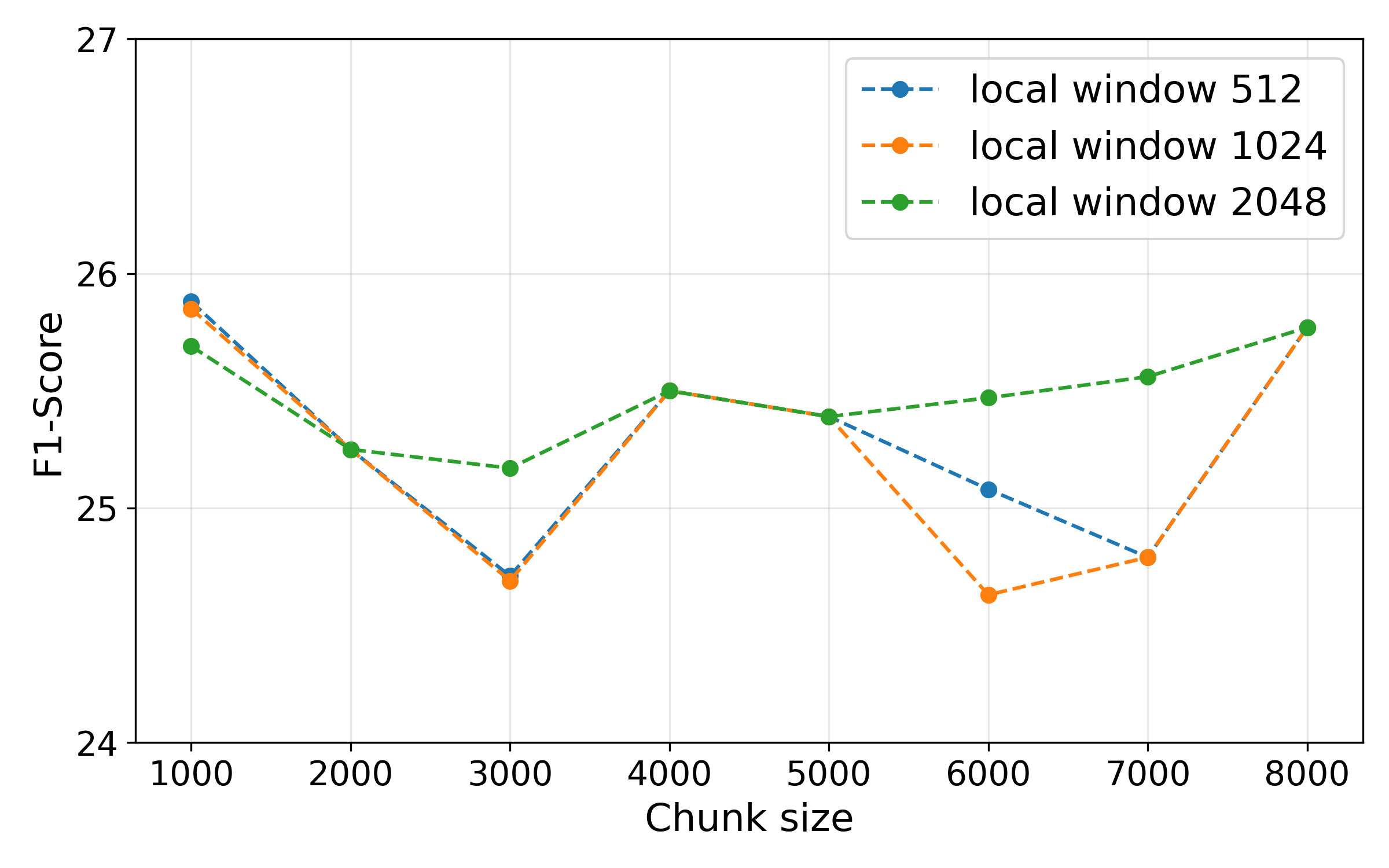
Figure 5: Impact of local window and chunk size on performance. The experiments use the Llama3-8b-ins-8k, with an extrapolated context window of 16384 tokens.

4.5 Ablation Studies

In this section, we investigate the impact of local window size and chunk size on GALI. We conducted our experiments using NarrativeQA, the longest dataset in LongBench. The results are shown in Figure 5. First, we observe that the differences across the three local window sizes are minimal, indicating that attention logit interpolation effectively approximates the true attention score distribution.

Secondly, as the chunk size increases, we hypothesize that the observed effects result from the interplay of two factors. Initially, a smaller chunk size aligns better with GALI’s design, which prioritizes leveraging pretrained positional intervals as much as possible while minimizing the number of interpolations for each token. Consequently, when the chunk size increases, the number of pretrained positional intervals utilized by each token decreases, while the number of interpolated positional intervals increases, leading to performance degradation.

However, as the chunk size grows, more tokens have their positional intervals compressed into a smaller range. As analyzed earlier, performing denser interpolations within a smaller positional interval range, such as [0, 4096), yields better results than performing sparser interpolations over a larger positional interval range, such as [0, 8192). Therefore, the performance of GALI begins to improve as the chunk size further increases.

5 Conclusion

In this paper, we introduced Greedy Attention Logit Interpolation (GALI), a novel training-free length extrapolation method, and evaluated it against other approaches across widely used real-world long-context tasks, long-context language modeling, and attention distribution analysis, demonstrating its superiority. The experiment results further reveal that LLMs interpret positional intervals differently within their training context window, suggesting that length extrapolation within a smaller positional range may outperform the vanilla LLM—even for short-context tasks.

Originally designed for RoPE-based LLMs, GALI avoids direct position embedding computations, making it compatible with any LLM exhibiting long-term decay, such as ALiBi. Future work will explore its applicability to other position embedding mechanisms. However, GALI currently requires two passes of attention logit computation, introducing computational overhead and making it incompatible with flash attention. To address this, we aim to integrate interpolation estimation into flash attention and develop more efficient local interpolation techniques.

6 Impact Statement

GALI is a training-free length extrapolation method that enables LLMs to handle long-context tasks without requiring fine-tuning. It is compatible with various position embedding schemes, making it a flexible plug-and-play solution. Furthermore, we show that, in practical scenarios, interpolating within a smaller context window than the training context window can enhance performance across both long-context and short-context downstream tasks.

Appendix A Pseudo code of GALI

In this section, we provide the pseudo-code for the key steps required to implement GALI. Algorithm 1 generates the chunk sizes needed to partition the input during the prefill phase. While this function can be modified to support dynamic chunk sizes, we use fixed chunk sizes in our experiments to better control memory usage. Algorithm 2 interpolates new position IDs based on the minimum number of new IDs required for each chunk. Algorithm LABEL:Interpolated_attention_logits demonstrates how we perform attention logit interpolation. Note that we use $r=\lceil{m}\rceil-n$ to represent the interval between $q_{m}$ and $k_{n}$. This is because, when computing attention logits using RoPE, we cannot directly manipulate the relative positional interval matrix; instead, we modify the relative positional interval matrix by separately operating on $query\_states$ and $key\_states$. By using $r=\lceil{m}\rceil-n$, we ensure that $\lfloor{r}\rfloor=\lceil{m}\rceil-\lceil{n}\rceil$ and $\lceil{r}\rceil=\lceil{m}\rceil-\lfloor{n}\rfloor$, enabling modifications to the relative positional interval matrix while preserving the relative order between $query\_states$ and $key\_states$. It is important to note that some operations, such as reshaping, which do not affect the core concept, are omitted from the pseudo-code in these three algorithms.

Algorithm 1 Generate Chunk Size List

0: $prefill\_len$: The length of input in the prefill phase, $L_{tr}$: Training context window, $s$: Chunk size

0: A list of chunk sizes that sums to $prefill\_len$

1: $chunk\_size\_list\leftarrow[L_{tr}]$

2: $sum\_len\leftarrow L_{tr}$

3: while $sum\_len<prefill\_len$ do

4:  Append $s$ to $chunk\_size\_list$

5:  $sum\_len\leftarrow sum\_len+s$

6: end while

7: Adjust the last chunk size:

8: $chunk\_size\_list[-1]\leftarrow chunk\_size\_list[-1]-(sum\_len-prefill\_len)$

9: return $chunk\_size\_list$

Algorithm 2 Position ID Interpolation

0: $cur\_len$: Current length of the sequence, $L_{tr}$: Training context window, $add\_token$: The number of positions to be interpolated, $L_{w}$: Neighbor window size

0: $new\_pi$: New position IDs

1: $target\_len\leftarrow cur\_len+add\_token$

2: $min\_group\_size\leftarrow\lceil(target\_len-L_{w})/(L_{tr}-L_{w})\rceil$

3: $interval\leftarrow 1/min\_group\_size$

4: $total\_len\leftarrow L_{tr}$

5: Initialize $new\_pi\leftarrow[]$ and $i\leftarrow 0$

6: while $total\_len<target\_len$ do

7:  Append $[i+interval\cdot j\mid j\in\{0,1,\dots,min\_group\_size-1\}]$ to $new\_pi$

8:  $i\leftarrow i+1$

9:  $total\_len\leftarrow L_{tr}-i+\text{len}(new\_pi)$

10: end while

11: $seg\_window\leftarrow[j\mid j\in\{i,i+1,\dots,L_{tr}-1\}]$

12: $new\_pi\leftarrow new\_pi[:(target\_len-\text{len}(seg\_window))]+seg\_window$

13: return $new\_pi$

Algorithm 3 Attention Logit Interpolation

0: $position\_ids$: Interpolated position IDs, $hidden\_states$: The inputs of the attention layer, $head\_dim$: The dimension of each head, q_proj: Q project function, k_proj: K project function, rotary_emb: Rotary embedding function

0: Interpolated attention logits # Compute the rotary embedding

1: $cos\_ceil,sin\_ceil\leftarrow\text{rotary\_emb}(hidden\_states,\lceil position\_ids\rceil)$

2: $cos\_floor,sin\_floor\leftarrow\text{rotary\_emb}(hidden\_states,\lfloor position\_ids\rfloor)$ # Apply the rotary embedding on the query and key states

3: $query\_states\leftarrow\text{q\_proj}(hidden\_states)$

4: $key\_states\leftarrow\text{k\_proj}(hidden\_states)$

5: $query\_states\_ceil\leftarrow(query\_states\cdot cos\_ceil)+(\text{rotate\_half}(query\_states)\cdot sin\_ceil)$

6: $key\_states\_ceil\leftarrow(key\_states\cdot cos\_ceil)+(\text{rotate\_half}(key\_states)\cdot sin\_ceil)$

7: $key\_states\_floor\leftarrow(key\_states\cdot cos\_floor)+(\text{rotate\_half}(key\_states)\cdot sin\_floor)$ # Compute attention logits with $\lceil{R}\rceil and\lfloor{R}\rfloor$

8: $attn\_floor\leftarrow query\_states\_ceil\text{@}key\_states\_ceil^{T}/\sqrt{head\_dim}$

9: $attn\_ceil\leftarrow query\_states\_ceil\text{@}key\_states\_floor^{T}/\sqrt{head\_dim}$

10: $rel\_coef\leftarrow(\lceil position\_ids\rceil.unsqueeze(1)-position\_ids.unsqueeze(0))\mod 1$

11: $attn\_logits\leftarrow attn\_floor-(attn\_floor-attn\_ceil)\cdot rel\_coef$ # Add normal distribution noise

12: $distance\_ids\leftarrow[i\mid i\in\{0,1,\dots,\text{len}(hidden\_states)-1\}]$

13: $distance\_matrix\leftarrow distance\_ids.unsqueeze(1)-distance\_ids.unsqueeze(0)$

14: $noise\_std\leftarrow distance\_matrix/\text{len}(hidden\_states)$

15: $noise\leftarrow\text{torch.randn\_like}(attn\_logits)$

16: $mask\leftarrow(rel\_coef\neq 0)$

17: $noise\leftarrow noise\cdot noise\_std\cdot mask$

18: $attn\_logits\leftarrow attn\_logits+noise$

19: return $attn\_logits$

Appendix B Data stastics

In this section, we provide detailed information about each dataset used in LongBench and L-Eval. Table LABEL:tab:benchmark_task_type presents the word length, task type, and number of samples for each dataset. Figure 6(a) and 6(b) show the length distributions of each dataset using the Llama2 and Llama3 tokenizers, respectively.

Benchmark	Dataset	Task Type	Avg Len	#Sample
LongBench	NarrativeQA	Single-doc QA	18409	200
	Qasper	Single-doc QA	3619	200
	MultiField-en	Single-doc QA	4559	150
	HotpotQA	Multi-doc QA	9151	200
	2WikiMQA	Multi-doc QA	4887	200
	Musique	Multi-doc QA	11214	200
	GovReport	Summarization	8734	200
	QMSum	Summarization	10614	200
	MultiNews	Summarization	2113	200
	TREC	Few shot	5177	200
	TriviaQA	Few shot	8209	200
	SAMSum	Few shot	6258	200
	PassageCount	Synthetic	11141	200
	PassageRe	Synthetic	9289	200
	LCC	Code	1235	500
	RepoBench-P	Code	4206	500
L-Eval	Coursera	Multiple choice	9075	172
L-Eval	GSM (16-shot)	Solving math problems	5557	100
	QuALITY	Multiple choice	7169	202
	TOEFL	Multiple choice	3907	269
	SFCition	True or False Questions	16381	64
	CodeU	Deducing program outputs	31575	90

Table 4: We list the task type, average word lengths, and the number of samples for each dataset we used in our work.

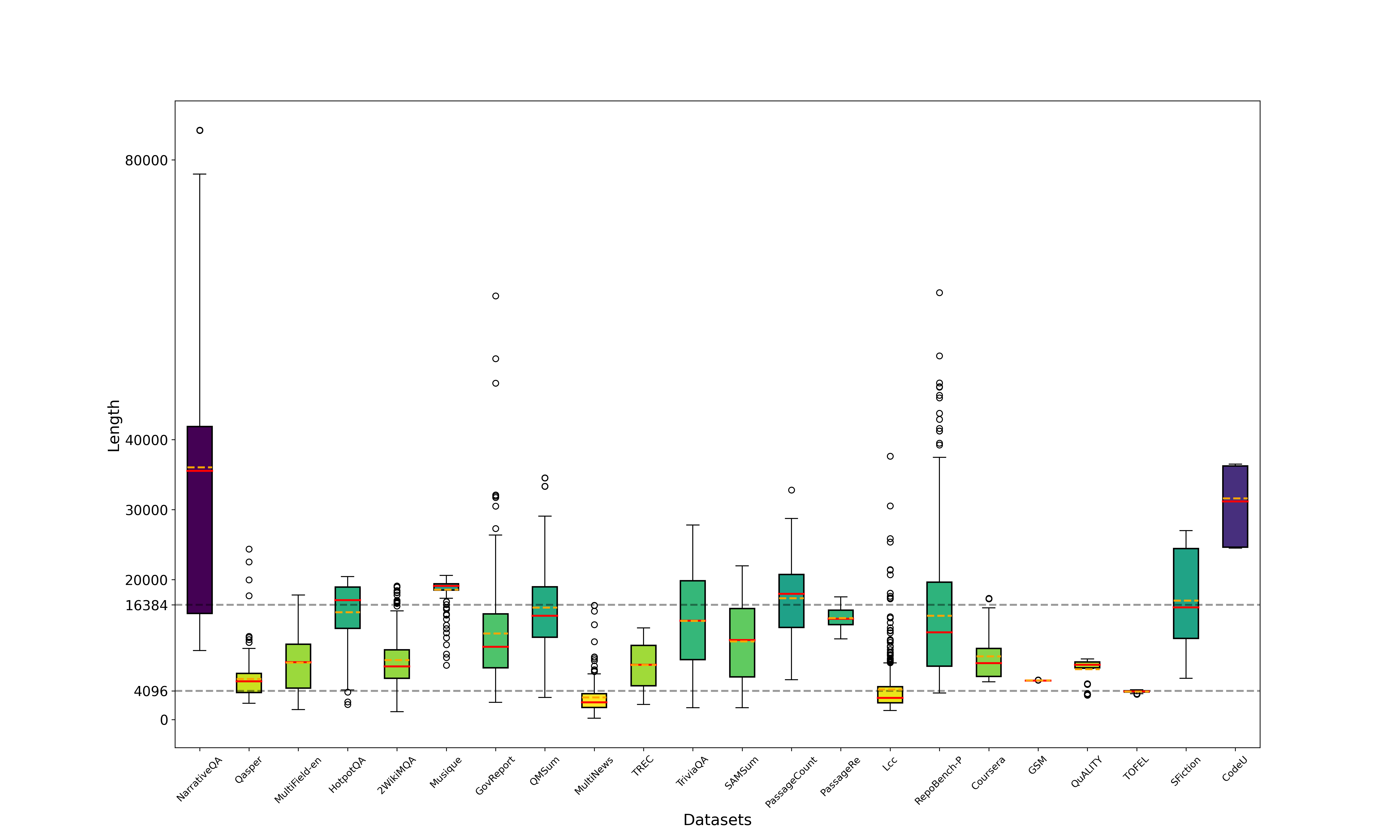
(a) Llama2 Tokenizer

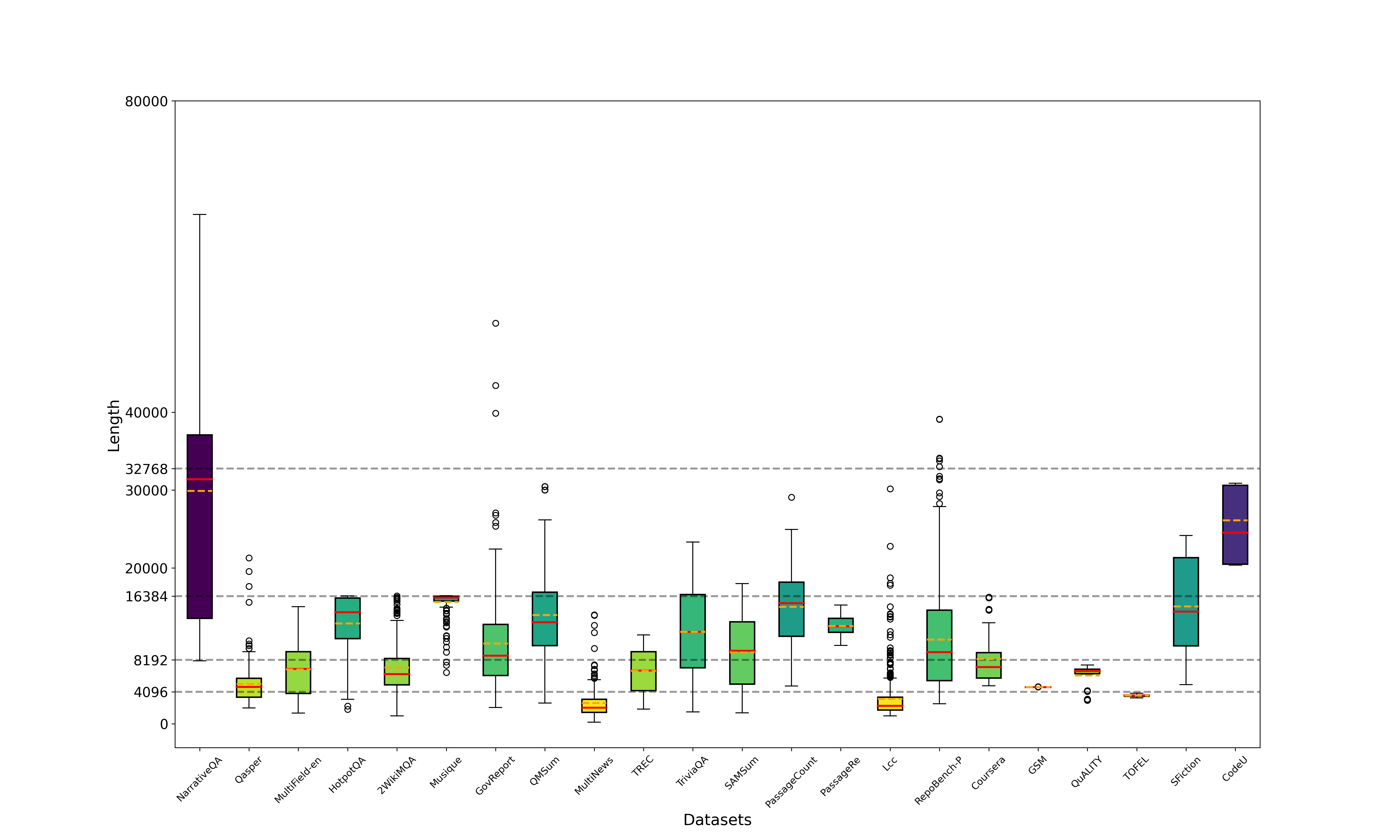
(b) Llama3 Tokenizer

Figure 6: Length distributions using Llama2 and Llama3 tokenizers. The left figure shows the distribution with Llama2, and the right figure shows the distribution with Llama3. The red line represents the median, the orange dashed line represents the mean, and the darker the color of the box, the greater the average length.

Appendix C Implementation details

In this section, we provide detailed implementation information for each method. For Dyn-NTK and YaRN, we utilize the implementations available in Huggingface by adding rope_scaling = {”rope_type”:”dynamic”} and rope_scaling = {”rope_type”:”yarn”}, respectively, to the LLM’s config.json file. For NTK, we implement it by adding rope_scaling = {”rope_type”:”dynamic”} and static_ntk=True, and modifying the _dynamic_frequency_update function of the LlamaRotaryEmbedding class as follows:

⬇

def _dynamic_frequency_update(self, position_ids, device):

"""

␣␣␣␣Modify␣this␣function␣to␣make␣it␣suitable␣for␣NTK

␣␣␣␣"""

if self.config.static_ntk == True:

if getattr(self, "reset_static_ntk", False) == False:

config = copy.deepcopy(self.config)

seq_len = self.original_max_seq_len * config.rope_scaling[’factor’]

config.rope_scaling[’factor’] = 1

inv_freq, self.attention_scaling = self.rope_init_fn(

config, device, seq_len=seq_len, **self.rope_kwargs

)

self.register_buffer("inv_freq", inv_freq, persistent=False)

setattr(self, "reset_static_ntk", True)

return

seq_len = torch.max(position_ids) + 1

if seq_len > self.max_seq_len_cached: # growth

inv_freq, self.attention_scaling = self.rope_init_fn(

self.config, device, seq_len=seq_len, **self.rope_kwargs

)

self.register_buffer("inv_freq", inv_freq, persistent=False) # TODO joao: may break with compilation

self.max_seq_len_cached = seq_len

if seq_len < self.original_max_seq_len and self.max_seq_len_cached > self.original_max_seq_len: # reset

self.register_buffer("inv_freq", self.original_inv_freq, persistent=False)

self.max_seq_len_cached = self.original_max_seq_len

For SelfExtend and ChunkLlama, we use their official implementations. We list the hyperparameters required for these methods to extend to different maximum input length in Table 5. All experiments can be conducted on a single A100 GPU (80GB) machine.

Length Extrapolation	Method	Hyperparameters
2k to 8k	NTK	rope_scaling={”rope type”:”dynamic”, ”factor”: 4}, static_ntk=True
	Dyn-NTK	rope_scaling={”rope type”:”dynamic”, ”factor”: 4}
	YaRN	rope_scaling={”rope type”:”YaRN”, ”factor”: 4}
	SelfExtend	group_size=5, window_size=512
	ChunkLlama	chunk_size=1536, local_window=128
	GALI	chunk_size=[1000,2000,3000], local_window=[128, 256, 512, 1024]
4k to 8k	NTK	rope_scaling={”rope type”:”dynamic”, ”factor”: 2}, static_ntk=True
	Dyn-NTK	rope_scaling={”rope type”:”dynamic”, ”factor”: 2}
	YaRN	rope_scaling={”rope type”:”YaRN”, ”factor”: 2}
	SelfExtend	group_size=3, window_size=2048
	ChunkLlama	chunk_size=3072, local_window=256
	GALI	chunk_size=[1000,2000,3000], local_window=[128, 256, 512, 1024]
4k to 16k	NTK	rope_scaling={”rope type”:”dynamic”, ”factor”: 4}, static_ntk=True
	Dyn-NTK	rope_scaling={”rope type”:”dynamic”, ”factor”: 4}
	YaRN	rope_scaling={”rope type”:”YaRN”, ”factor”: 4}
	SelfExtend	group_size=5, window_size=1024
	ChunkLlama	chunk_size=3072, local_window=256
	GALI	chunk_size=[1000,2000,3000], local_window=[128, 256, 512, 1024]
4k to 32k	NTK	rope_scaling={”rope type”:”dynamic”, ”factor”: 8}, static_ntk=True
	Dyn-NTK	rope_scaling={”rope type”:”dynamic”, ”factor”: 8}
	YaRN	rope_scaling={”rope type”:”YaRN”, ”factor”: 8}
	SelfExtend	group_size=15, window_size=2048
	ChunkLlama	chunk_size=3072, local_window=256
	GALI	chunk_size=[1000,2000,3000], local_window=[128, 256, 512, 1024]
8k to 16k	NTK	rope_scaling={”rope type”:”dynamic”, ”factor”: 2}, static_ntk=True
	Dyn-NTK	rope_scaling={”rope type”:”dynamic”, ”factor”: 2}
	YaRN	rope_scaling={”rope type”:”YaRN”, ”factor”: 2}
	SelfExtend	group_size=3, window_size=4096
	ChunkLlama	chunk_size=6144, local_window=512
	GALI	chunk_size=[1000,2000,3000], local_window=[128, 256, 512, 1024]
8k to 32k	NTK	rope_scaling={”rope type”:”dynamic”, ”factor”: 4}, static_ntk=True
	Dyn-NTK	rope_scaling={”rope type”:”dynamic”, ”factor”: 4}
	YaRN	rope_scaling={”rope type”:”YaRN”, ”factor”: 4}
	SelfExtend	group_size=5, window_size=2048
	ChunkLlama	chunk_size=6144, local_window=512
	GALI	chunk_size=[1000,2000,3000], local_window=[128, 256, 512, 1024]

Table 5: Hyperparameters for length extrapolation methods under each setting. For example, “2k to 8k” indicates an initial context window of 2048, with a positional interval range of [0, 2048), and a target context window extending up to 8192. Other settings follow the same pattern. For GALI, the reported hyperparameters represent the combinations we search for each experiment.

Appendix D Extra experiment results

D.1 Real-world long-context task results

We conducted experiments on LongBench and L-Eval using the Llama2-4k backbone, as shown in Tables 6 and 7. On LongBench, GALI performed similarly to NTK, Dyn-NTK, and YaRN, but was weaker than SelfExtend and ChunkLlama. However, all methods performed significantly worse than those using the Llama3-8b-ins-4k backbone.

Although Llama2-7b-chat and Llama3-8b-ins have similar parameter scales, Llama3 demonstrates a deeper understanding of pretrained positional intervals closer to its training context window. Consequently, GALI performed significantly better on Llama3-8b-ins-4k than on Llama2-4k, with similar trends observed across other methods. As the quality of the pretrained model improves, it better aligns with GALI’s principle of maximizing the use of pretrained positional intervals.

Regarding the best-performing method on Llama2-4k, SelfExtend has been reported to be highly sensitive to hyperparameters (Jin et al., 2024). Specifically, larger group sizes and smaller local windows sometimes yield better results, which supports our conclusion in Section 4.2. These configurations emphasize the use of smaller positional intervals, reducing reliance on larger ones and preventing content from being placed in less well-understood positional intervals. This limitation affects GALI’s effectiveness on Llama2, as GALI assumes the model fully understands its entire training context window, thereby always maximizing the use of pretrained positional intervals.

On the L-Eval benchmark, the performance gap between GALI and the best approaches was smaller than on LongBench. This is because, when using the Llama2 tokenizer, datasets such as Coursera, GSM, QuALITY, and TOEFL in L-Eval are much shorter than 16k, allowing all methods to leverage Llama2-4k’s well-understood smaller relative positional intervals. In longer datasets like SFictions and CodeU, performance is task-dependent. SFictions is a True/False task with higher results, while CodeU is a code inference task with much lower results. We also report complete results using the Llama3-8k backbone. Our method performed almost identically to the backbone model, as the token lengths of GSM, QuALITY, and TOEFL are all below 8192. However, SelfExtend, NTK, and YaRN outperformed the backbone model, further validating our conclusion that even on short text datasets, using a smaller range of positional intervals for length extrapolation leads to better task performance.

	Methods	Single document QA			Multi document QA			Summarization			Few-shot Learning			Synthetic		Code		Average
		NarrativeQA	Qasper	MultiField-en	HotpotQA	2WikiMQA	Musique	GovReport	QMSum	MultiNews	TREC	TriviaQA	SAMSum	PassageCount	PassageRe	Lcc	RepoBench-P
Llama2-7b-chat-4k	Original*	18.70	19.20	36.80	25.40	32.80	9.40	27.30	20.80	25.80	61.50	77.80	40.70	2.10	9.80	52.40	43.80	31.52
	Original	8.48	13.97	20.4	13.62	16.77	5.46	25.17	12.47	24.78	67.5	74.24	40.28	2.30	3.25	56.39	50.36	27.22
	SelfExtend-16k*	21.69	25.02	35.21	34.34	30.24	14.13	27.32	21.35	25.78	69.50	81.99	40.96	5.66	5.83	60.60	54.33	34.62
	SelfExtend-16k	6.89	12.67	25.95	9.08	11.25	5.88	26.80	16.39	22.79	67.50	69.88	41.18	2.18	3.21	58.21	51.65	26.97
	ChunkLlama-16k	8.48	13.97	20.40	13.62	16.77	5.46	25.17	12.47	24.78	67.50	74.24	40.28	2.30	3.25	56.39	50.36	27.22
	NTK-16k	0.73	10.33	19.44	2.38	7.91	0.42	19.47	6.26	26.13	59.50	17.89	23.17	0.52	0.51	50.70	27.91	17.08
	Dyn-NTK-16k	3.79	10.37	22.38	7.47	10.26	3.81	29.52	20.13	22.84	63.50	45.35	31.79	2.29	4.33	57.13	42.16	23.57
	YaRN-16k	3.22	10.86	22.14	5.52	13.36	1.32	24.78	10.90	25.92	64.50	40.60	32.36	2.20	2.15	51.74	43.91	22.22
	(Ours)GALI-16k	6.29	16.73	22.26	12.82	13.65	6.31	23.58	15.96	23.37	62.00	72.80	25.12	1.83	2.83	58.71	48.51	25.80

Table 6: Performance comparison with different backbone LLMs and training-free length extrapolation methods. The best result in each experiment has been bolded. ^* indicates the results reported by LongBench(Bai et al., 2024), ^* indicates the results reported by LongBench(Jin et al., 2024). The number following each method represents the target context window. For example, 16k means 16 × 1024. The ”Original” means testing with the backbone model, i.e., the model shown in the left column.

	Methods	Coursera	GSM	QuALITY	TOFEL	SFiction	CodeU	Average
Llama2-7b-chat-4k	Original*	29.21	19.00	37.62	51.67	60.15	1.11	33.12
	Original	29.80	29.00	37.62	58.36	60.16	1.11	36.01
	SelfExtend-16k*	35.76	25.00	41.09	55.39	57.81	1.11	36.02
	SelfExtend-16k	32.99	29.00	40.59	57.62	57.81	2.22	36.71
	ChunkLlama*	32.12	31.00	35.14	57.62	61.72	2.22	36.64
	ChunkLlama-16k	28.92	31.00	43.07	58.36	60.94	2.22	37.42
	NTK-16k*	32.71	19.00	33.16	52.78	64.84	0.00	33.75
	NTK-16k	26.89	16.00	33.66	60.97	41.41	0.00	29.82
	Dyn-NTK*	13.95	13.00	30.69	52.27	57.02	1.11	28.01
	Dyn-NTK-16k	15.41	13.00	33.17	54.65	54.69	1.11	28.67
	YaRN-16k	36.49	18.00	42.08	57.62	42.97	7.78	34.15
	(Ours)GALI-16k	35.32	29.00	39.11	54.65	51.43	4.44	35.66
Llama3-8b-ins-8k	Original	53.05	58.00	61.88	82.16	60.16	4.44	53.93
	SelfExtend-16k	55.38	63.00	62.87	82.16	64.06	5.56	55.76
	ChunkLlama*	56.24	54.00	63.86	83.27	70.31	5.56	55.54
	ChunkLlama-16k	53.34	54.00	60.89	81.78	61.72	5.56	53.53
	NTK-16k	52.03	77.00	65.35	81.04	42.97	0.00	56.58
	Dyn-NTK-16k	52.03	55.00	61.88	82.16	52.34	2.22	52.89
	YaRN-16k	55.96	75.00	63.37	79.93	62.50	5.56	57.83
	(Ours)GALI-16k	54.65	59.09	61.88	83.33	65.63	6.67	55.42
Llama3-8b-ins-8k	SelfExtend-32k	53.92	77.00	63.37	79.93	65.63	3.33	57.20
	ChunkLlama-32k	54.36	55.00	60.89	81.78	64.06	5.56	53.61
	NTK-32k	58.28	83.00	63.86	81.04	59.38	1.11	57.78
	Dyn-NTK-32k	54.36	55.00	61.88	82.16	64.06	6.67	54.02
	YaRN-32k	55.23	76.00	62.38	79.18	67.19	7.78	57.96
	(Ours)GALI-32k	54.17	59.09	62.38	82.68	66.41	7.78	55.29

Table 7: Performance comparison with different backbone LLMs and training-free length extrapolation methods. The best result in each experiment has been bolded. ^* indicates the results reported by ChunkLlama(An et al., 2024b), ^* indicates the results reported by LongBench(Jin et al., 2024), and ^* indicates the results reported by L-Eval(An et al., 2024a).

D.2 Long language modeling task results

We also conducted PPL evaluations on the Llama2-7b-chat-4k backbone. As shown in Table 8, GALI maintained a stable PPL, while Dyn-NTK consistently produced the worst results.

	Methods	1k	2k	3k	4k	5k	6k	7k	8k
Llama3-7b-chat-4k	SelfExtend	8.81	8.99	9.16	9.24	9.25	9.16	9.2	9.3
	ChunkLlama	9.07	9.26	9.41	9.45	9.43	9.31	9.31	9.39
	NTK	8.95	9.04	9.16	9.18	9.16	9.06	9.26	13.67
	Dyn-NTK	8.81	8.99	9.15	10.79	44.32	87.35	160.07	224.07
	YaRN	11.65	8.97	9.07	9.16	9.17	9.15	9.03	9.04
	(Ours)GALI	8.81	8.99	9.15	9.24	9.59	9.66	9.63	9.66

Table 8: Performance of various methods on PG19 Dataset with different context windows, using Llama2-7b-chat-4k as the backbone model.

D.3 Attention distribution analysis results

In this section, we present the detailed results of the attention distribution analysis. First, we compare the differences between the attention score matrix of length extrapolation methods and the standard attention score matrix, as shown in Figure LABEL:attn_score_dist. For this analysis, we averaged the attention score matrices for each layer and each head before comparison. Whether comparing Llama3-2k or Llama3-4k, GALI consistently achieved the highest similarity to the standard attention score matrix. Additionally, we observed that all methods exhibited higher values in the lower-left corner of the matrix compared to the standard attention score matrix. We attribute this to the fact that these methods do not perform true extrapolation, whereas the standard Llama3-8k model, utilizing a larger positional interval range [0, 8192), results in a lower mean value of the attention scores.

We also analyzed the attention score distribution by extracting 8 rows from the attention score matrix, with the results shown in Figures 5 and 6. The figures clearly demonstrate that GALI’s attention score distribution for each row is closer to the corresponding original attention score distribution. Moreover, as the row index increases, the attention score distributions of all length extrapolation methods show an upward shift relative to the original attention score distribution. This aligns with our earlier analysis, as using a smaller positional interval range results in higher mean value of the attention scores.

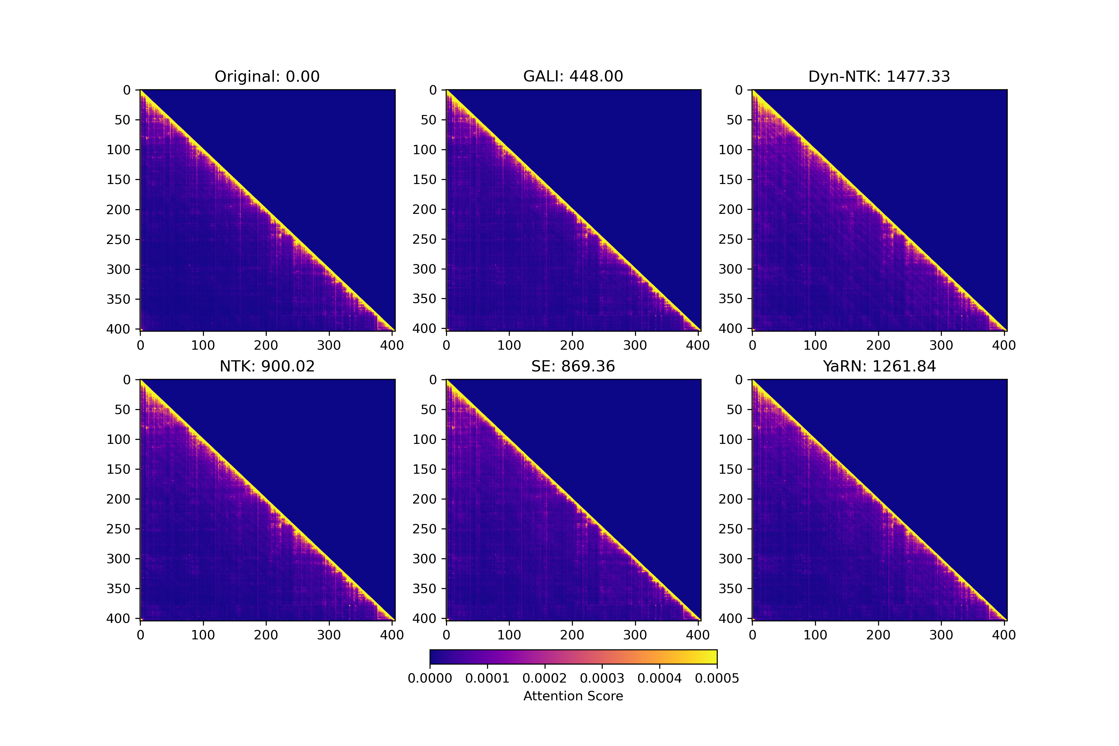
(a) Llama3-8b-ins-2k backbone

(b) Llama3-8b-ins-4k backbone

Figure 7: This is a comparison of the attention score matrices obtained using Llama3-2k and Llama3-4k for length extrapolation with those of Llama3-8k. Note that we averaged the attention scores across all layers and heads, applied average pooling to scale the matrix to 0.05%, and set the maximum value of the heatmap to 0.0005 for better visualization. “Original” represents the attention score matrix of Llama3-8k, and the number next to each method’s name indicates the sum of the absolute differences between the method’s attention scores matrices and the “Original” matrix.

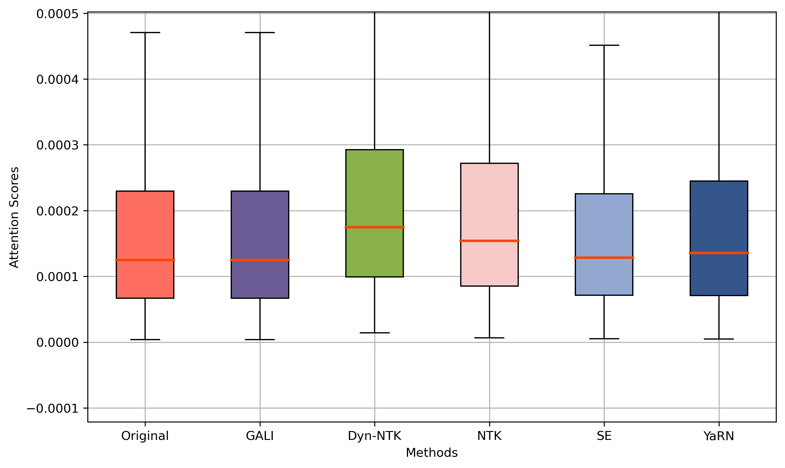
(a) Attention scores of row 1000

(b) Attention scores of row 2000

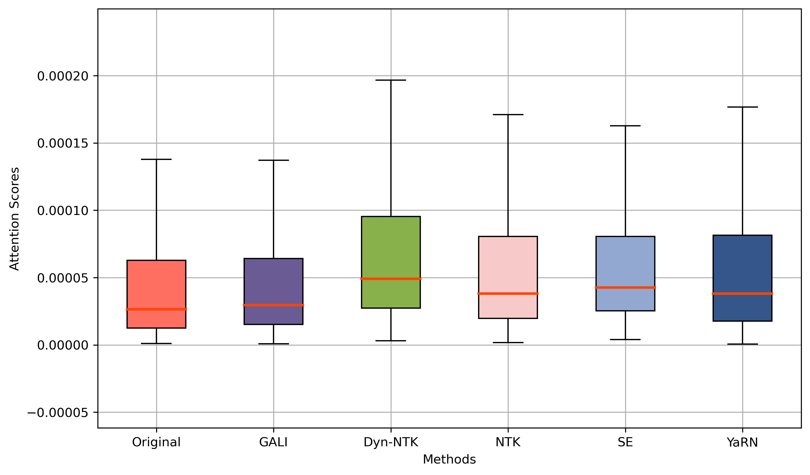
(c) Attention scores of row 3000

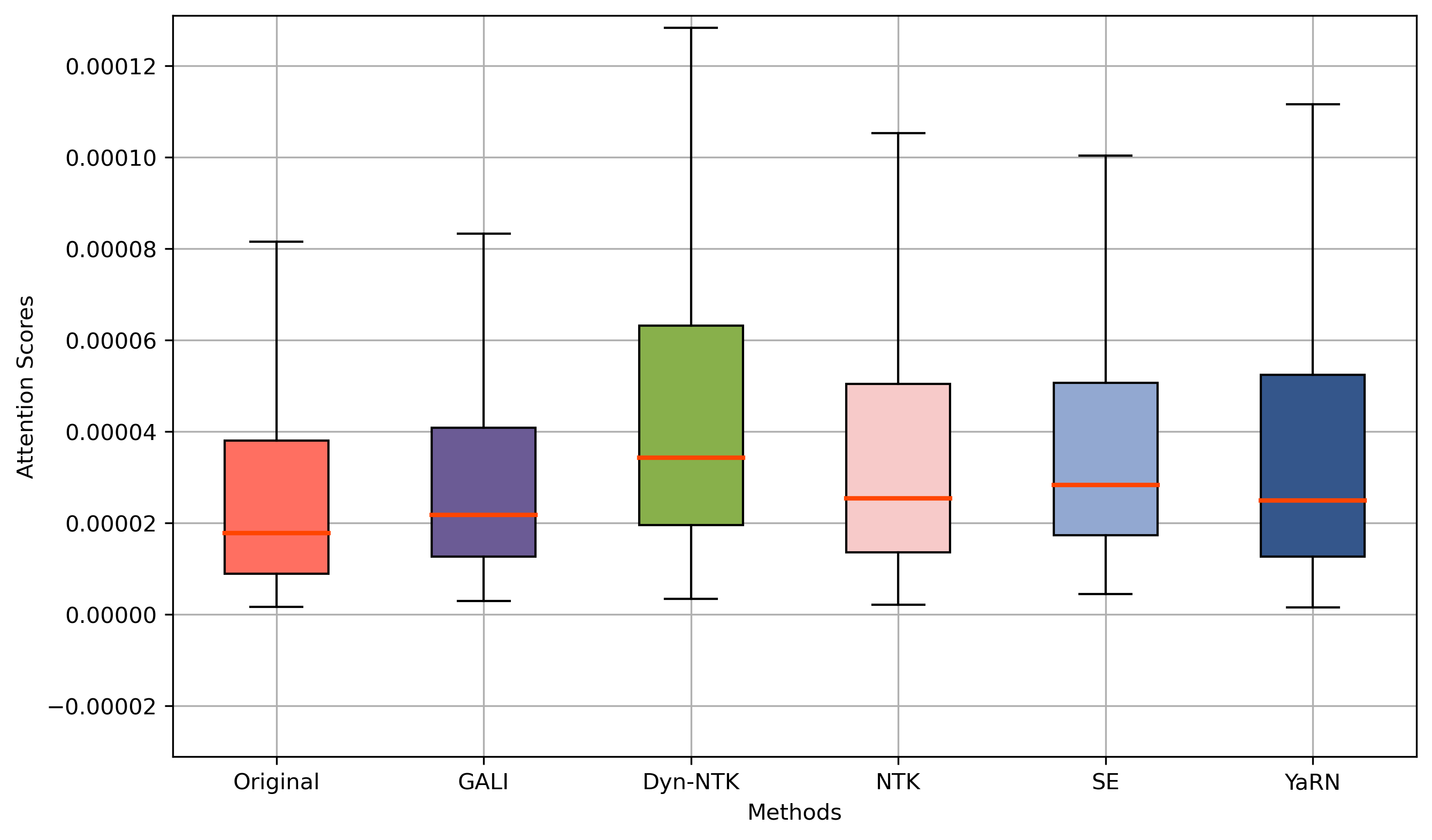
(d) Attention scores of row 4000

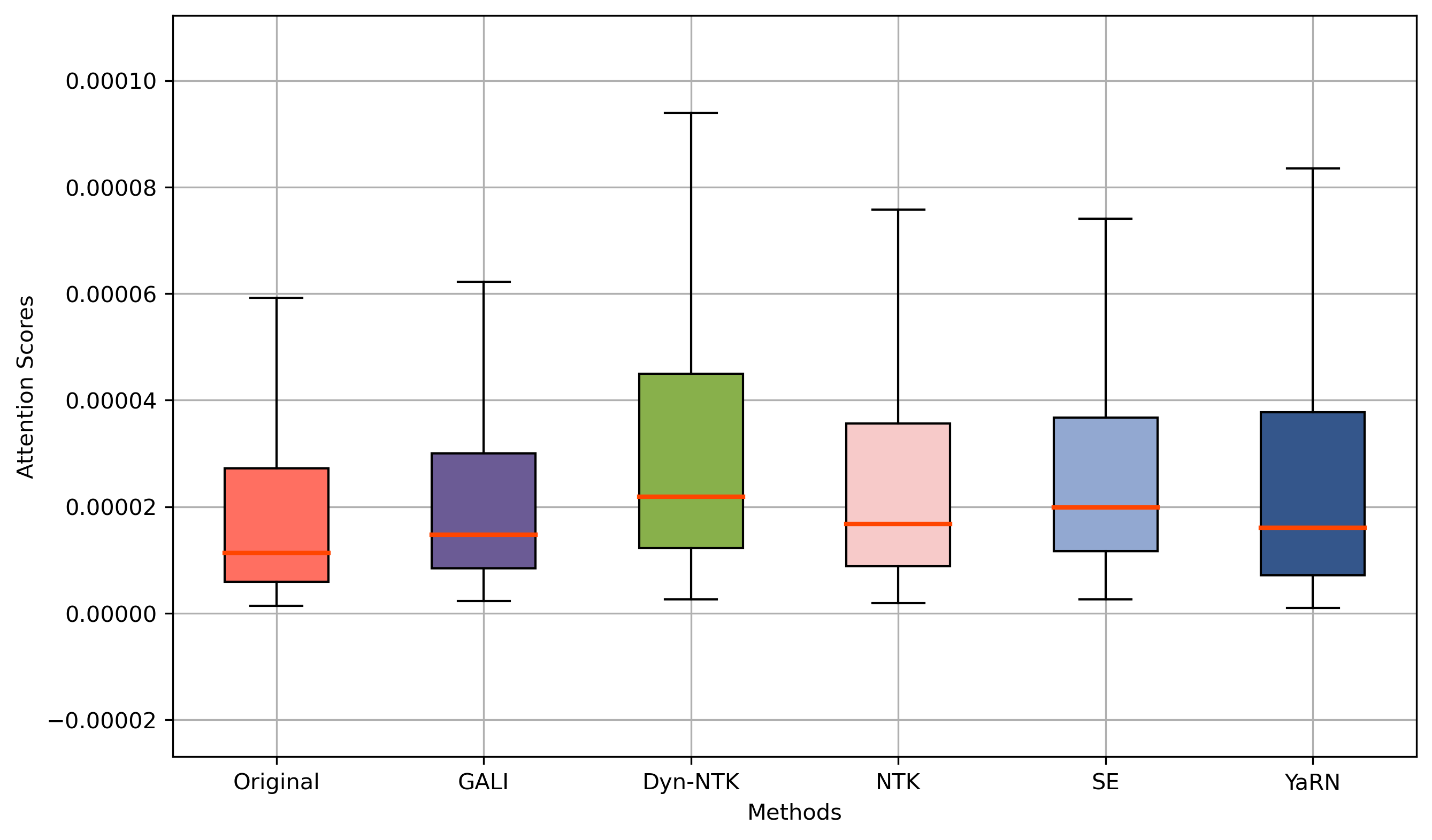
(e) Attention scores of row 5000

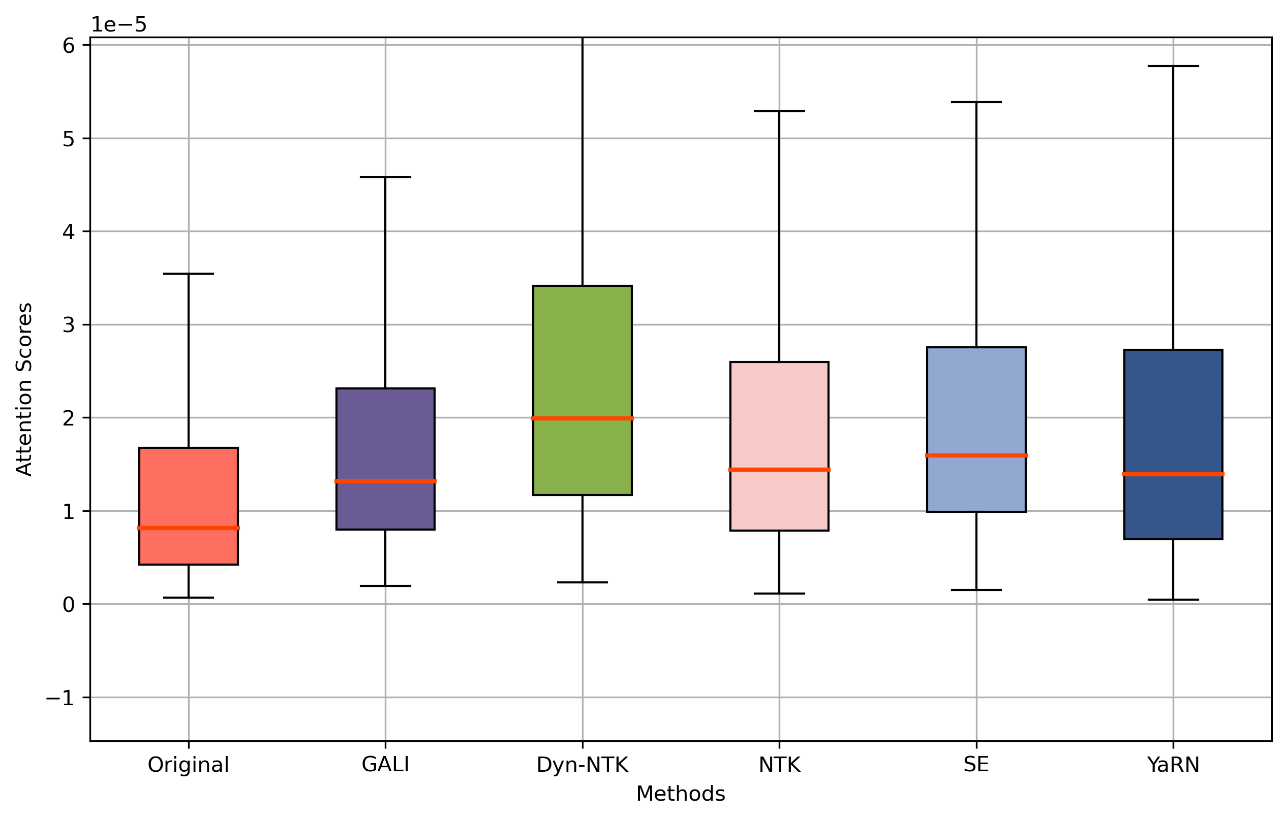
(f) Attention scores of row 6000

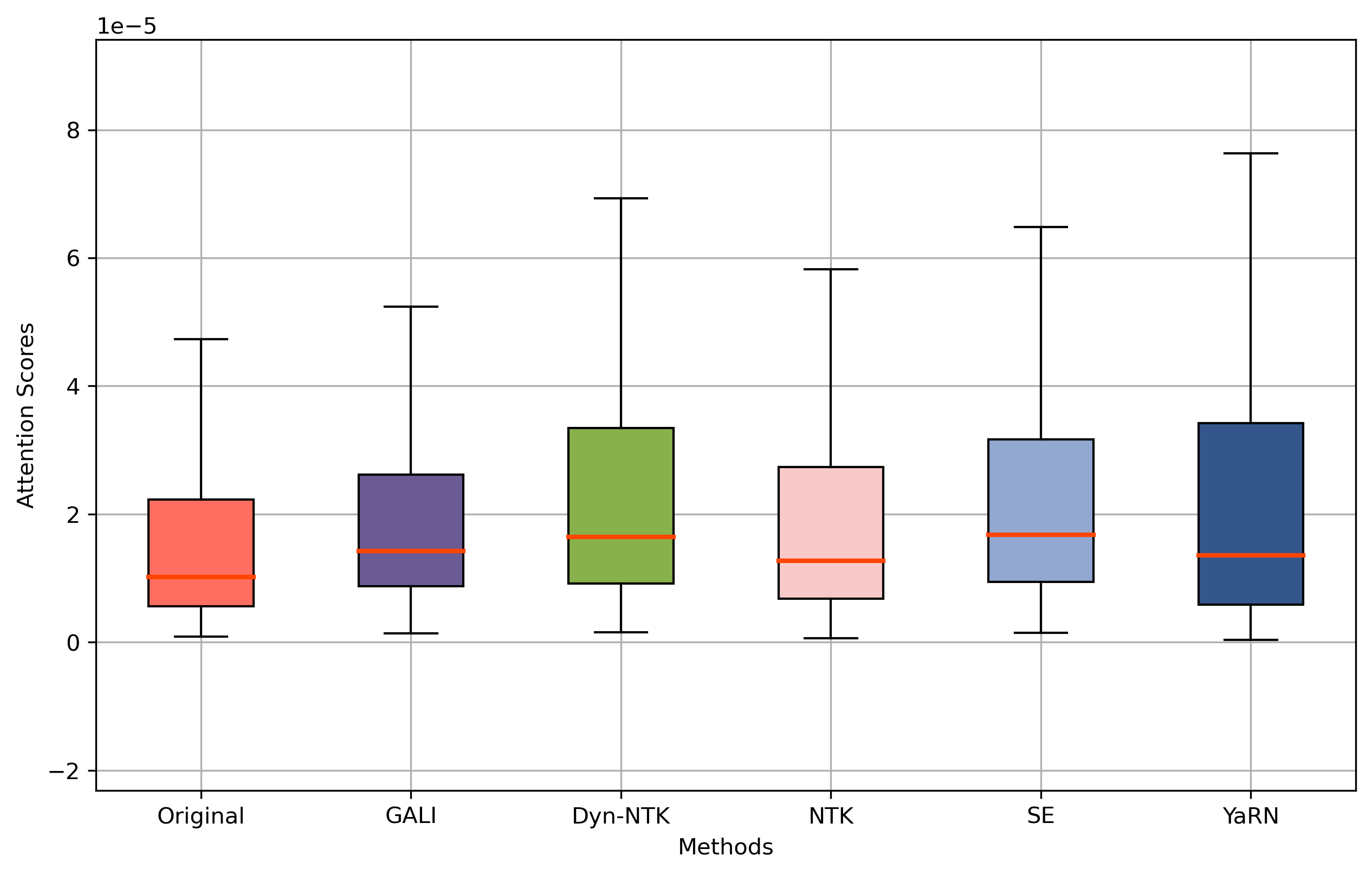
(g) Attention scores of row 7000

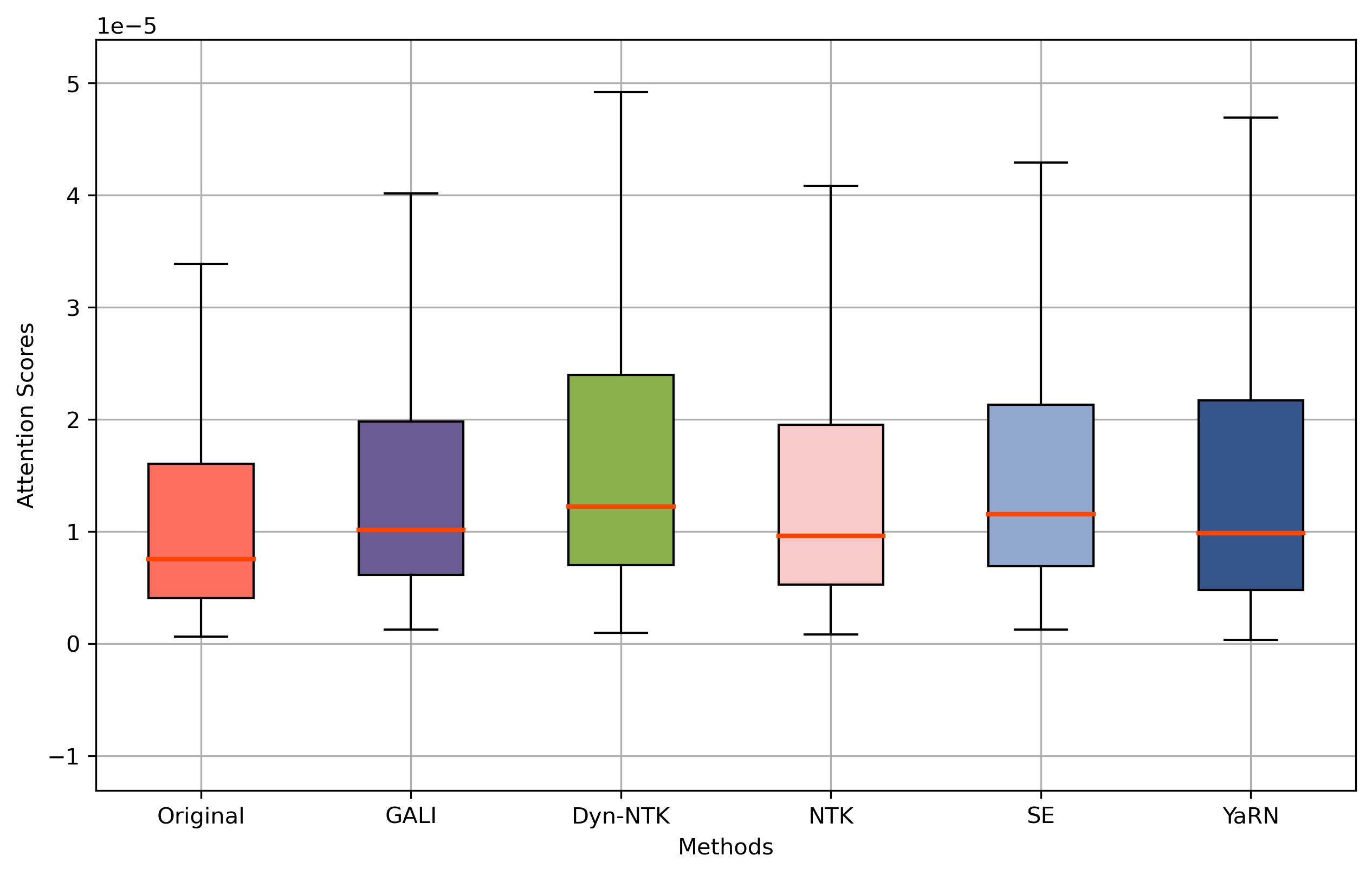
(h) Attention scores of row 8000

Figure 8: Attention score distribution using Llama3-2k backbone. We omitted attention scores outside the 1st percentile and the 90th percentile here for clearer visualization.

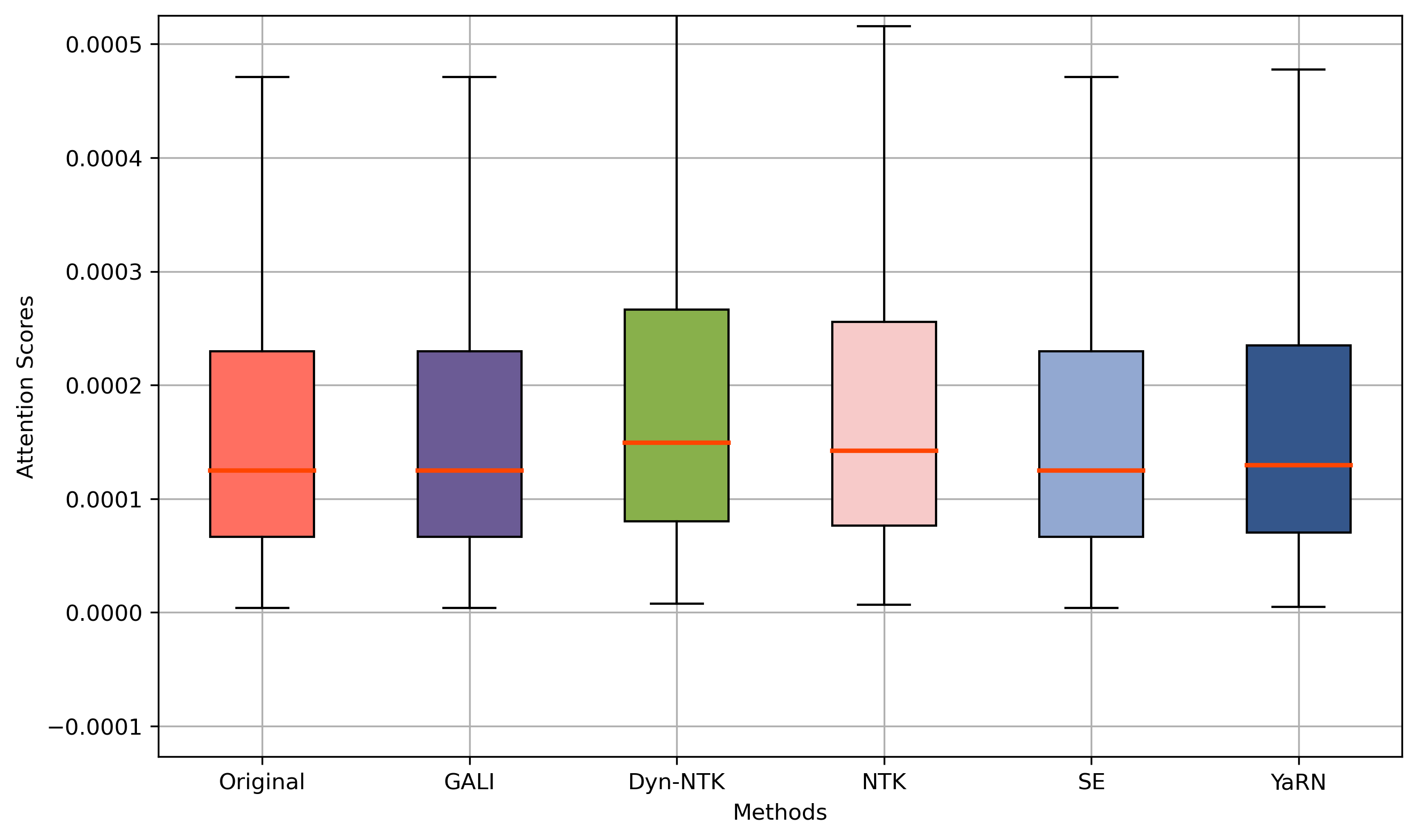
(a) Attention scores of row 1000

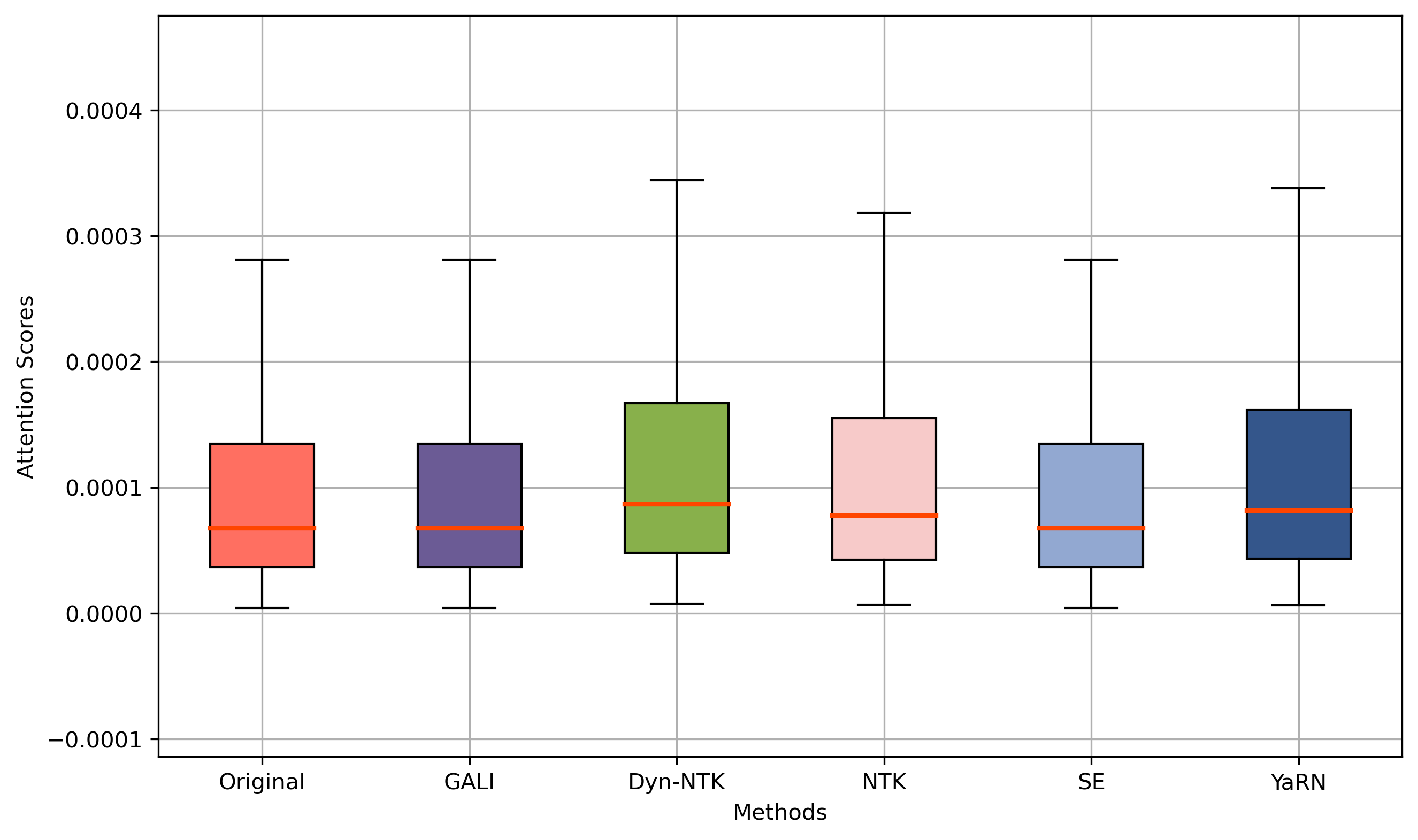
(b) Attention scores of row 2000

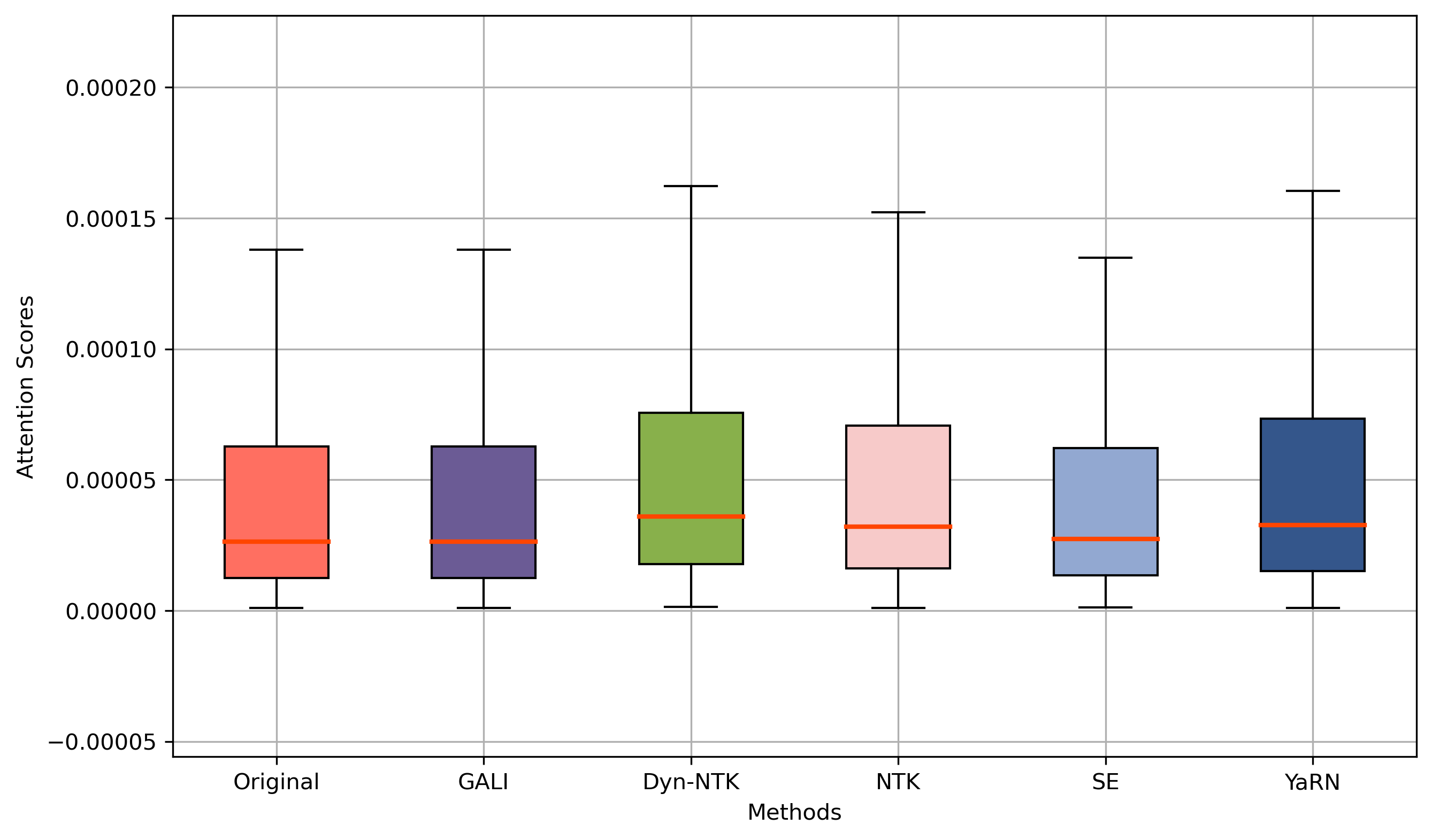
(c) Attention scores of row 3000

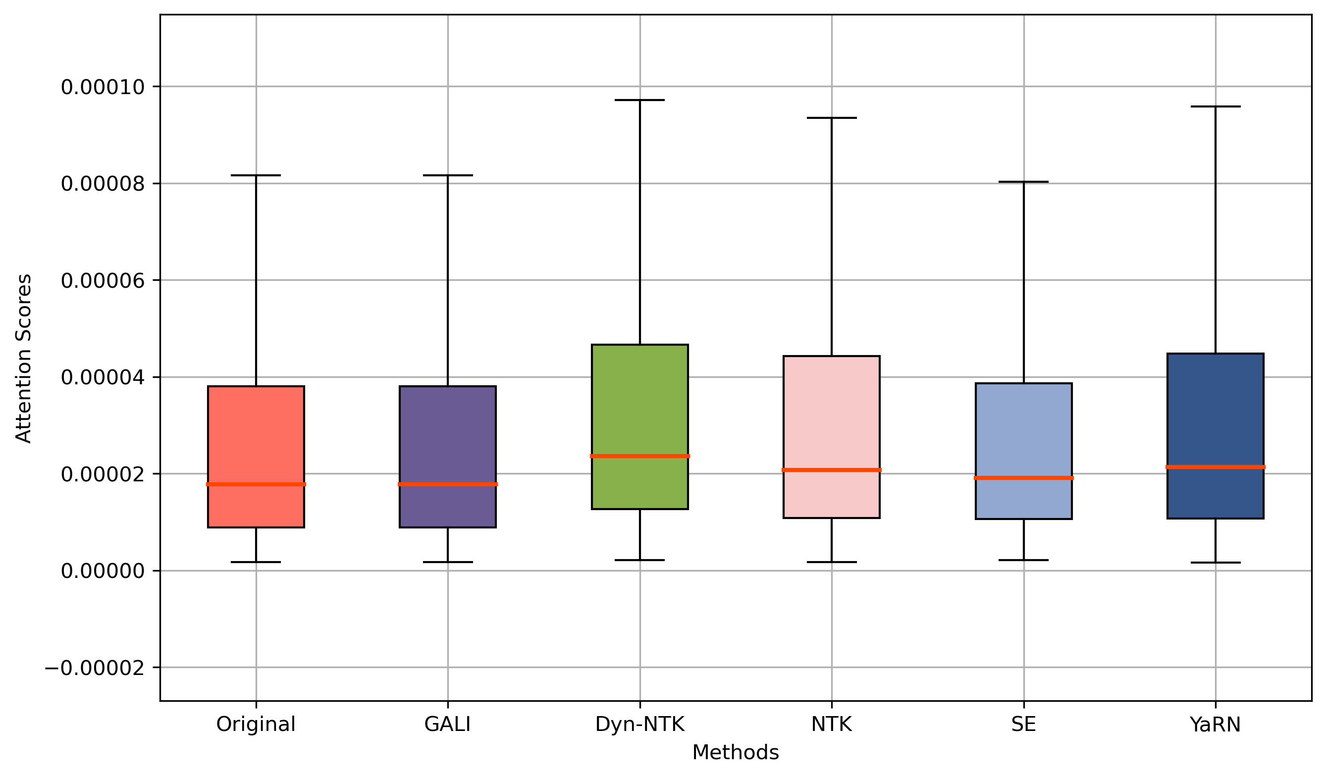
(d) Attention scores of row 4000

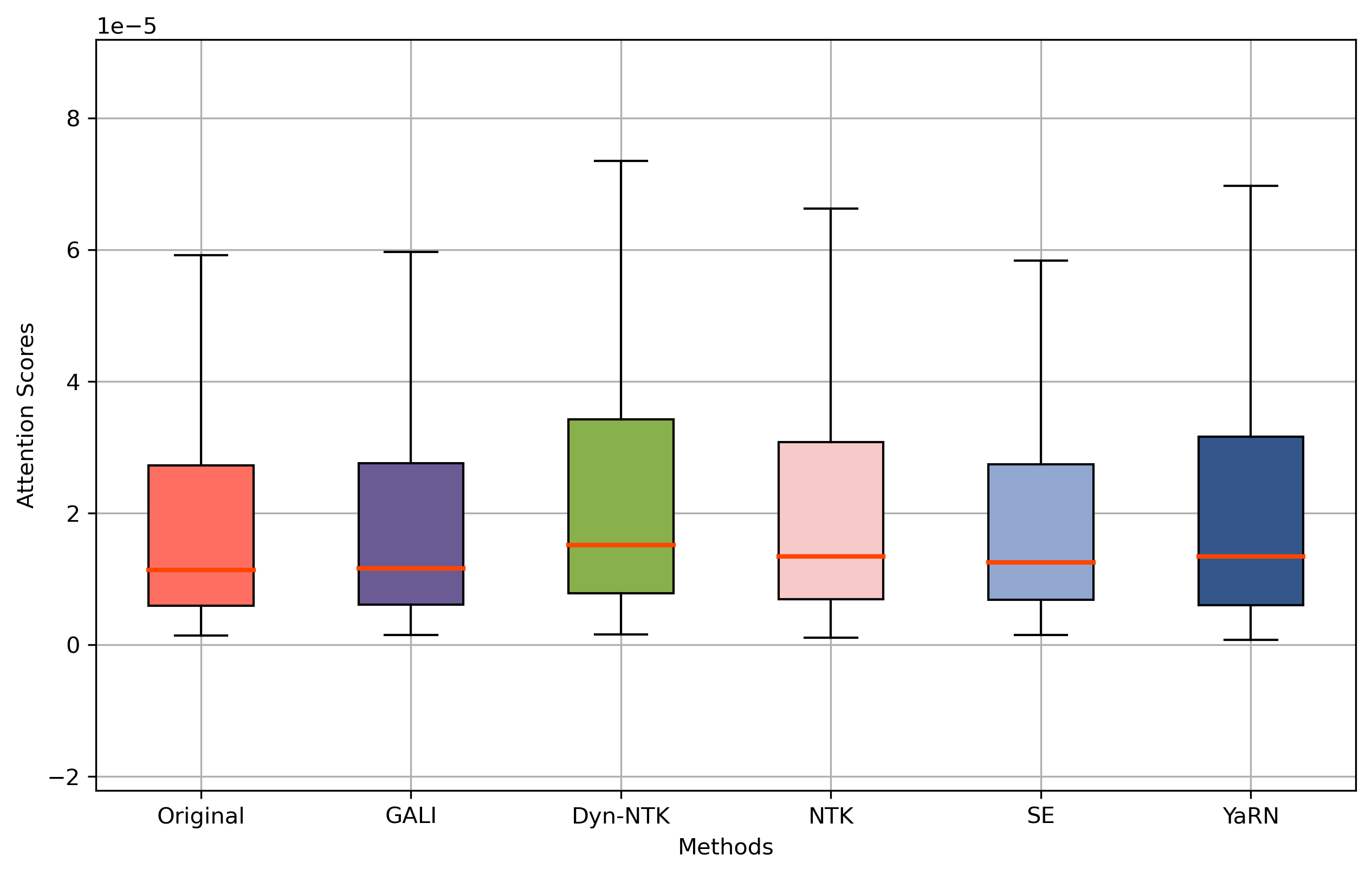
(e) Attention scores of row 5000

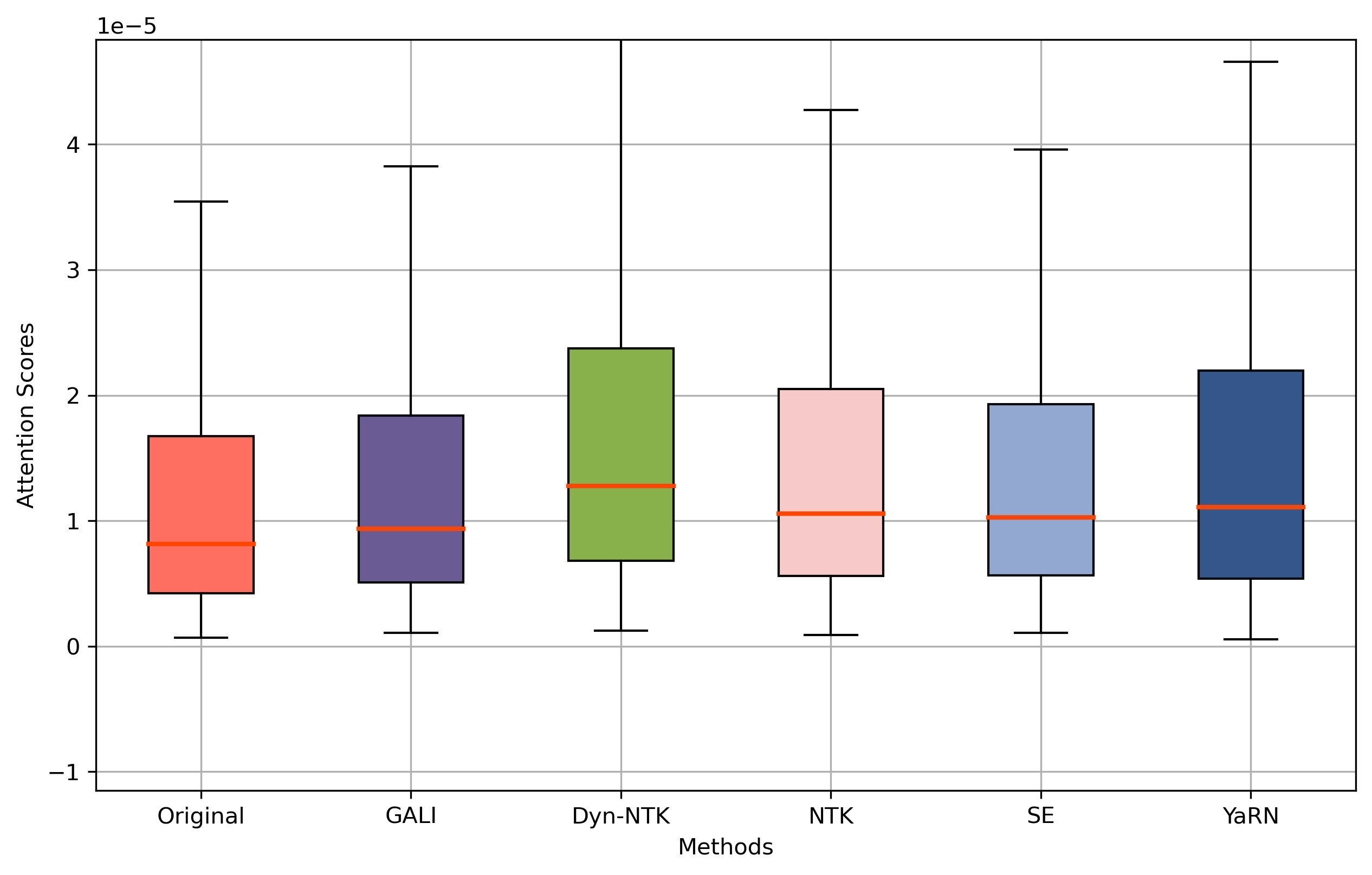
(f) Attention scores of row 6000

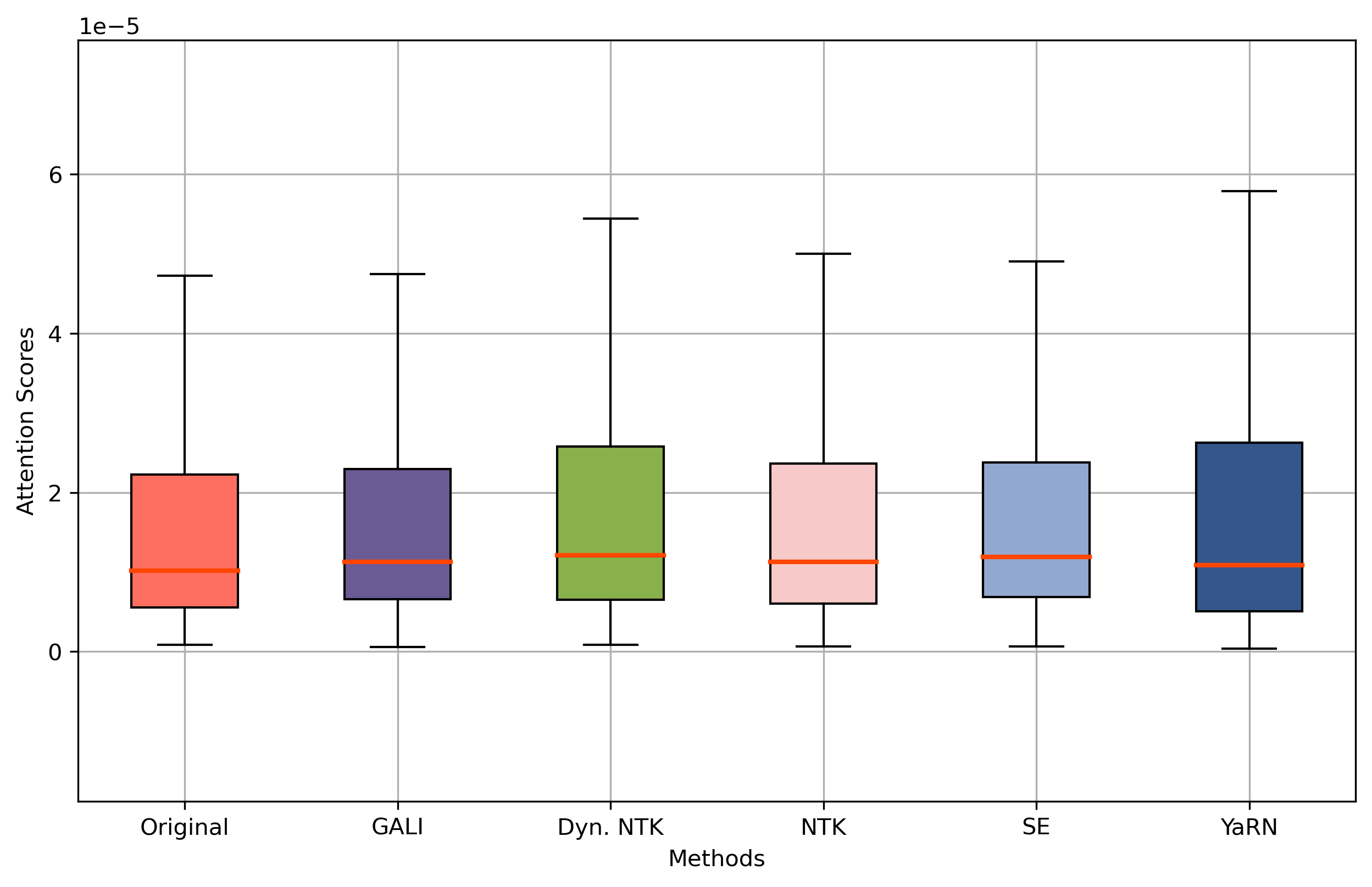
(g) Attention scores of row 7000

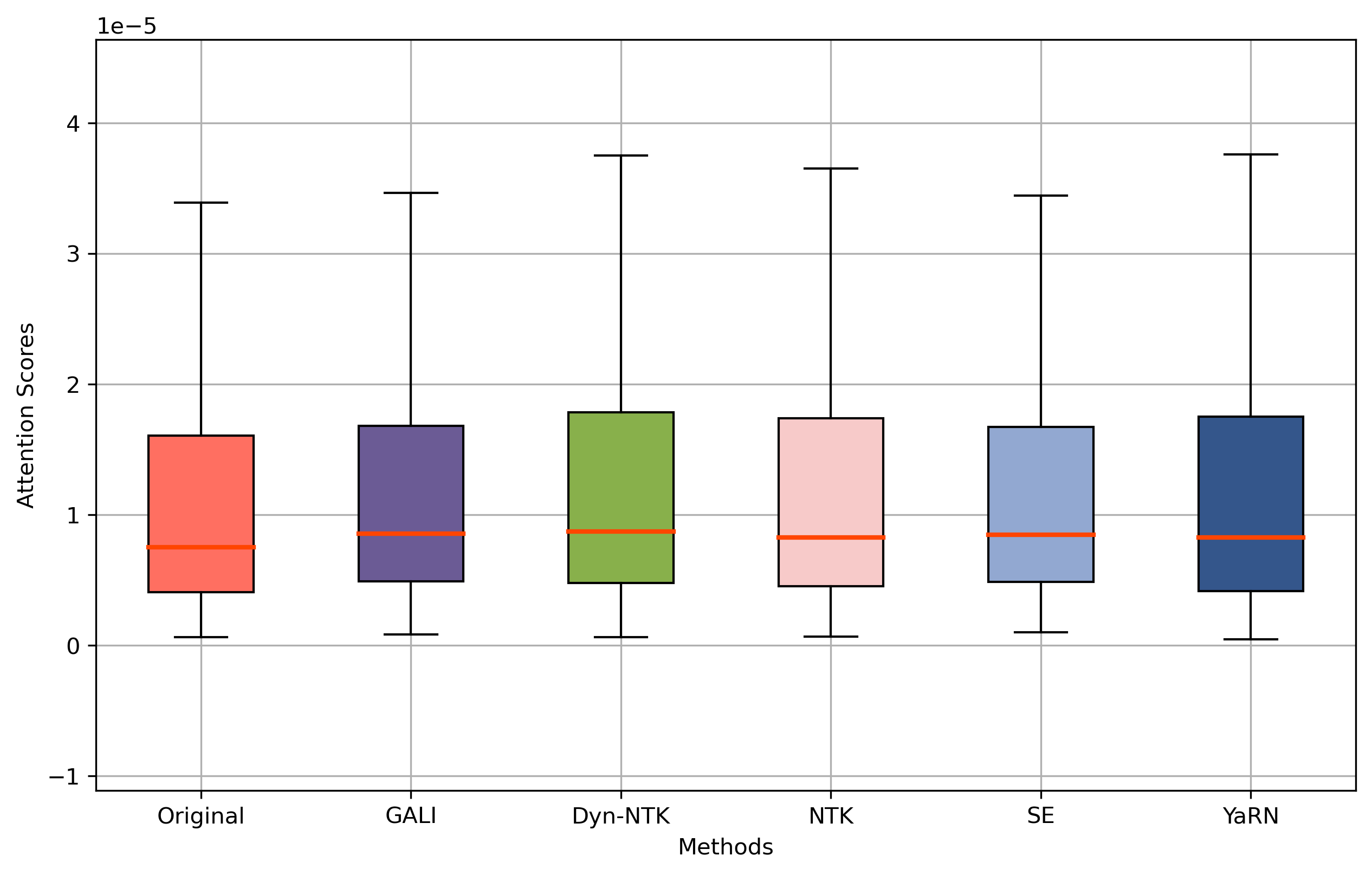
(h) Attention scores of row 8000

Figure 9: Attention score distribution using Llama3-4k backbone. We omitted attention scores outside the 1st percentile and the 90th percentile here for clearer visualization.

References

- An et al. (2024a) An, C., Gong, S., Zhong, M., Zhao, X., Li, M., Zhang, J., Kong, L., and Qiu, X. L-eval: Instituting standardized evaluation for long context language models. In Ku, L.-W., Martins, A., and Srikumar, V. (eds.), Proceedings of the 62nd Annual Meeting of the Association for Computational Linguistics (Volume 1: Long Papers), pp. 14388–14411, Bangkok, Thailand, August 2024a. Association for Computational Linguistics. doi: 10.18653/v1/2024.acl-long.776. URL https://aclanthology.org/2024.acl-long.776/.
- An et al. (2024b) An, C., Huang, F., Zhang, J., Gong, S., Qiu, X., Zhou, C., and Kong, L. Training-free long-context scaling of large language models. arXiv preprint arXiv:2402.17463, 2024b.
- Bai et al. (2024) Bai, Y., Lv, X., Zhang, J., Lyu, H., Tang, J., Huang, Z., Du, Z., Liu, X., Zeng, A., Hou, L., Dong, Y., Tang, J., and Li, J. LongBench: A bilingual, multitask benchmark for long context understanding. In Ku, L.-W., Martins, A., and Srikumar, V. (eds.), Proceedings of the 62nd Annual Meeting of the Association for Computational Linguistics (Volume 1: Long Papers), pp. 3119–3137, Bangkok, Thailand, August 2024. Association for Computational Linguistics. doi: 10.18653/v1/2024.acl-long.172. URL https://aclanthology.org/2024.acl-long.172/.
- Chen et al. (2023a) Chen, G., Li, X., Meng, Z., Liang, S., and Bing, L. Clex: Continuous length extrapolation for large language models. arXiv preprint arXiv:2310.16450, 2023a.
- Chen et al. (2023b) Chen, S., Wong, S., Chen, L., and Tian, Y. Extending context window of large language models via positional interpolation. arXiv preprint arXiv:2306.15595, 2023b.
- Chen et al. (2023c) Chen, Y., Qian, S., Tang, H., Lai, X., Liu, Z., Han, S., and Jia, J. Longlora: Efficient fine-tuning of long-context large language models. ArXiv, abs/2309.12307, 2023c. URL https://api.semanticscholar.org/CorpusID:262084134.
- Ding et al. (2024) Ding, Y., Zhang, L. L., Zhang, C., Xu, Y., Shang, N., Xu, J., Yang, F., and Yang, M. Longrope: Extending llm context window beyond 2 million tokens. arXiv preprint arXiv:2402.13753, 2024.
- Dufter et al. (2021) Dufter, P., Schmitt, M., and Schütze, H. Position information in transformers: An overview. Computational Linguistics, 48:733–763, 2021. URL https://api.semanticscholar.org/CorpusID:231986066.
- Farquhar et al. (2024) Farquhar, S., Kossen, J., Kuhn, L., and Gal, Y. Detecting hallucinations in large language models using semantic entropy. Nature, 630(8017):625–630, 2024.
- Han et al. (2024) Han, C., Wang, Q., Peng, H., Xiong, W., Chen, Y., Ji, H., and Wang, S. Lm-infinite: Zero-shot extreme length generalization for large language models. In Proceedings of the 2024 Conference of the North American Chapter of the Association for Computational Linguistics: Human Language Technologies (Volume 1: Long Papers), pp. 3991–4008, 2024.
- Hsieh et al. (2024) Hsieh, C.-P., Sun, S., Kriman, S., Acharya, S., Rekesh, D., Jia, F., and Ginsburg, B. Ruler: What’s the real context size of your long-context language models? ArXiv, abs/2404.06654, 2024. URL https://api.semanticscholar.org/CorpusID:269032933.
- Jiang et al. (2024) Jiang, H., Li, Y., Zhang, C., Wu, Q., Luo, X., Ahn, S., Han, Z., Abdi, A. H., Li, D., Lin, C.-Y., et al. Minference 1.0: Accelerating pre-filling for long-context llms via dynamic sparse attention. arXiv preprint arXiv:2407.02490, 2024.
- Jin et al. (2024) Jin, H., Han, X., Yang, J., Jiang, Z., Liu, Z., yuan Chang, C., Chen, H., and Hu, X. Llm maybe longlm: Self-extend llm context window without tuning. ArXiv, abs/2401.01325, 2024. URL https://api.semanticscholar.org/CorpusID:266725385.
- Kazemnejad et al. (2024) Kazemnejad, A., Padhi, I., Natesan Ramamurthy, K., Das, P., and Reddy, S. The impact of positional encoding on length generalization in transformers. Advances in Neural Information Processing Systems, 36, 2024.
- Li et al. (2024a) Li, J., Shi, H., Jiang, X., Li, Z., Xu, H., and Jia, J. Quickllama: Query-aware inference acceleration for large language models. arXiv preprint arXiv:2406.07528, 2024a.
- Li et al. (2024b) Li, R., Xu, J., Cao, Z., Zheng, H.-T., and Kim, H.-G. Extending context window in large language models with segmented base adjustment for rotary position embeddings. Applied Sciences, 14(7):3076, 2024b.
- Li et al. (2023) Li, S., You, C., Guruganesh, G., Ainslie, J., Ontanon, S., Zaheer, M., Sanghai, S., Yang, Y., Kumar, S., and Bhojanapalli, S. Functional interpolation for relative positions improves long context transformers. arXiv preprint arXiv:2310.04418, 2023.
- LocalLLaMA (2023a) LocalLLaMA. Dynamically Scaled NTK-Aware RoPE, 2023a. URL https://www.reddit.com/r/LocalLLaMA/comments/14mrgpr/dynamically_scaled_rope_further_increases/.
- LocalLLaMA (2023b) LocalLLaMA. NTK-Aware Scaled RoPE, 2023b. URL https://www.reddit.com/r/LocalLLaMA/comments/14lz7j5/ntkaware_scaled_rope_allows_llama_models_to_have/.
- Peng et al. (2023) Peng, B., Quesnelle, J., Fan, H., and Shippole, E. Yarn: Efficient context window extension of large language models. arXiv preprint arXiv:2309.00071, 2023.
- Rae et al. (2019) Rae, J. W., Potapenko, A., Jayakumar, S. M., and Lillicrap, T. P. Compressive transformers for long-range sequence modelling. ArXiv, abs/1911.05507, 2019. URL https://api.semanticscholar.org/CorpusID:207930593.
- Su et al. (2024) Su, J., Ahmed, M., Lu, Y., Pan, S., Bo, W., and Liu, Y. Roformer: Enhanced transformer with rotary position embedding. Neurocomputing, 568:127063, 2024.
- Wu et al. (2024) Wu, T., Zhao, Y., and Zheng, Z. Never miss a beat: An efficient recipe for context window extension of large language models with consistent” middle” enhancement. arXiv preprint arXiv:2406.07138, 2024.
- Xiao et al. (2023) Xiao, G., Tian, Y., Chen, B., Han, S., and Lewis, M. Efficient streaming language models with attention sinks. arXiv preprint arXiv:2309.17453, 2023.
- Xiong et al. (2023) Xiong, W., Liu, J., Molybog, I., Zhang, H., Bhargava, P., Hou, R., Martin, L., Rungta, R., Sankararaman, K. A., Oğuz, B., Khabsa, M., Fang, H., Mehdad, Y., Narang, S., Malik, K., Fan, A., Bhosale, S., Edunov, S., Lewis, M., Wang, S., and Ma, H. Effective long-context scaling of foundation models. In North American Chapter of the Association for Computational Linguistics, 2023. URL https://api.semanticscholar.org/CorpusID:263134982.
- Xu et al. (2024) Xu, M., Men, X., Wang, B., Zhang, Q., Lin, H., Han, X., et al. Base of rope bounds context length. In The Thirty-eighth Annual Conference on Neural Information Processing Systems, 2024.
- Zhang et al. (2024) Zhang, Z., Wang, Y., Huang, X., Fang, T., Zhang, H., Deng, C., Li, S., and Yu, D. Attention entropy is a key factor: An analysis of parallel context encoding with full-attention-based pre-trained language models. arXiv preprint arXiv:2412.16545, 2024.
- Zhu et al. (2023) Zhu, D., Yang, N., Wang, L., Song, Y., Wu, W., Wei, F., and Li, S. Pose: Efficient context window extension of llms via positional skip-wise training. ArXiv, abs/2309.10400, 2023. URL https://api.semanticscholar.org/CorpusID:262053659.