Lieb-Robinson bounds with exponential-in-volume tails

Abstract

Lieb-Robinson bounds demonstrate the emergence of locality in many-body quantum systems. Intuitively, Lieb-Robinson bounds state that with local or exponentially decaying interactions, the correlation that can be built up between two sites separated by distance $r$ after a time $t$ decays as $\exp(vt-r)$, where $v$ is the emergent Lieb-Robinson velocity. In many problems, it is important to also capture how much of an operator grows to act on $r^{d}$ sites in $d$ spatial dimensions. Perturbation theory and cluster expansion methods suggest that at short times, these volume-filling operators are suppressed as $\exp(-r^{d})$ at short times. We confirm this intuition, showing that for $r>vt$, the volume-filling operator is suppressed by $\exp(-(r-vt)^{d}/(vt)^{d-1})$. This closes a conceptual and practical gap between the cluster expansion and the Lieb-Robinson bound. We then present two very different applications of this new bound. Firstly, we obtain improved bounds on the classical computational resources necessary to simulate many-body dynamics with error tolerance $\varepsilon$ for any finite time $t$: as $\varepsilon$ becomes sufficiently small, only $\varepsilon^{-\mathrm{O}(t^{d-1})}$ resources are needed. A protocol that likely saturates this bound is given. Secondly, we prove that disorder operators have volume-law suppression near the “solvable (Ising) point” in quantum phases with spontaneous symmetry breaking, which implies a new diagnostic for distinguishing many-body phases of quantum matter.

1 Introduction

The Lieb-Robinson Theorem Lieb and Robinson (1972) proves that quantum correlations and entanglement spread with at most a finite velocity in many-body quantum lattice models. While the original proof of this theorem is over 50 years old, it has recently become an extremely important technical tool in mathematical many-body physics Chen et al.(2023)(Anthony) Chen, Lucas, and Yin (Anthony). The Lieb-Robinson Theorem underlies proofs of (1) the efficient simulatability of quantum dynamics on classical or quantum computers Osborne (2006); Haah et al. (2021); (2) lower bounds on the time needed to prepare entangled states in quantum information processors Bravyi et al. (2006); Eisert and Osborne (2006), including those with power-law interactions Gong et al. (2017); Chen and Lucas (2019); Tran et al. (2019); Kuwahara and Saito (2020); Tran et al. (2020, 2021a); Hong and Lucas (2021); Kuwahara and Saito (2021a); Tran et al. (2021b); Guo et al. (2020); Yin (2024) and, in some cases, bosonic degrees of freedom Nachtergaele et al. (2008); Schuch et al. (2011); Jünemann et al. (2013); Kuwahara and Saito (2021b); Yin and Lucas (2022); Faupin et al. (2022a, b); Kuwahara et al. (2024); Vu et al. (2024); Lemm et al. (2023); (3) the prethermal robustness of gapped phases of matter Yin and Lucas (2023) and the non-perturbative metastability of false vacua Yin et al. (2024a); (4) the stability of topological order Hastings and Wen (2005); Bravyi et al. (2010); Michalakis and Zwolak (2013) and quantization of Hall conductance Hastings and Michalakis (2015); (5) the area-law of entanglement entropy in 1D Hastings (2007) (although there are also combinatorial proofs); (6) clustering of correlations in gapped ground states Hastings and Koma (2006); Nachtergaele and Sims (2006); (7) robustness of quantum metrology Yin and Lucas (2024a); Yin et al. (2024b) (see Chen et al.(2023)(Anthony) Chen, Lucas, and Yin (Anthony) for a more complete list of applications). Besides these mathematical results, the intuition gained from the Lieb-Robinson bound has been important in developing a new theory of many-body quantum chaos in lattice models, where the onset of chaotic behavior at early times is characterized by the growth of a Heisenberg-evolved operator from a short string of Pauli matrices to a long string Nahum et al. (2018); von Keyserlingk et al. (2018). This growth is controlled by a similar “Frobenius light cone”, which generally has a smaller velocity than the Lieb-Robinson light cone Tran et al. (2020). For this reason, insight from a precise understanding of quantum operator growth may lead to improved classical algorithms to simulate hydrodynamics Rakovszky et al. (2022).

This diversity of applications, spanning quantum information sciences, atomic physics, condensed matter and even high-energy physics, usually relies on a Lieb-Robinson Theorem stated as follows: given two local operators $A_{x}$ and $B_{y}$, and a local many-body lattice model,

$$\lVert[A_{x}(t),B_{y}]\rVert\lesssim\exp[\mu(vt-|x-y|)]$$ (1)

where $|x-y|$ denotes the distance between the degrees of freedom and $\mu$ is a constant. This bound is good enough for many of the applications listed above. To give one example of how the simple bound (1) would be used, let us briefly discuss how to bound the classical simulatability of quantum dynamics. Suppose we wish to study the Heisenberg-evolved operator $A_{x}(t)$ by solving the Heisenberg equation of motion for $A_{x}$. Given finite computational resources, we simply truncate the list of Pauli strings we keep track of to those supported in a ball of radius $R$ around site $x$. We will refer to this truncated operator as the “fraction” of the operator acting within this ball. In $d$ spatial dimensions, the number of such operators scales as $N\sim\exp[R^{d}]$. (1) suggests that the error in this approximation $\varepsilon$ will be bounded by $\varepsilon\lesssim\exp[\mu(vt-R)]$. The classical resources necessary to simulate dynamics can thus be estimated as

$$N\sim\exp\left[\left(vt+\frac{1}{\mu}\log\frac{1}{\varepsilon}\right)^{d}\right].$$ (2)

For the rest of the introduction, O(1) prefactors in scaling relations will be suppressed.

The argument above—as do many other applications of a Lieb-Robinson bound—crucially relies on the exponential decay in distance in (1). Is that optimal? As phrased in (1), the bound is pretty much optimal: the tail bound can be improved to at most $\exp(-R\log R)$ with strictly local interactions Chen et al.(2023)(Anthony) Chen, Lucas, and Yin (Anthony). This can be intuitively seen by noting that at order $R$, the operator $A_{x}(t)$ can grow $R$ sites away:

$$A_{x}(t)=A_{x}+\mathrm{i}t[H_{x+1,x},A_{x}]+\cdots+\frac{(\mathrm{i}t)^{R}}{R!}[H_{x+R,x+R-1},[\cdots,[H_{x+1,x},A_{x}]]]+\cdots.$$ (3)

On the other hand, when we bounded simulatability in $d>1$, we use a Lieb-Robinson bound for the spreading of an operator from $x$ to $y$, and assumed that this same error controls how much of the operator might act on the whole ball of radius $|x-y|$. This approximation might seem loose. Indeed, (3) suggests that the first terms that act on an entire ball of radius $R$ arise at order $R^{d}$, so we might expect a tail bound that is suppressed in volume: $\exp(-R^{d})$. Lieb-Robinson bounds of this kind are not known. However, the simulatability of short-time dynamics starting from product states has been directly addressed using a rather different method (cluster expansion), and an algorithm requiring

$$N\sim\exp\left[\mathrm{e}^{t}\log\varepsilon^{-1}\right]$$ (4)

has been found Wild and Alhambra (2023). For fixed $t$ and $\varepsilon\rightarrow 0$, (4) is better; while for fixed $\varepsilon$ and large $t$, (2) is better. The large mismatch in scaling with $t$ and $\varepsilon$ suggests that neither is optimal. To find an optimal bound for this application, and for many others, it is crucial to have better control over the shape of $A_{x}(t)$ outside of the “Lieb-Robinson light cone”—the region within distance $vt$ of the initial site $x$. This paper will address precisely this problem.

2 Summary of results

Our central objective is to better understand the “tail” of an operator—the fraction that acts outside the light cone. Quantum circuits with local gates have strict light cones, so time-evolved operators have no tails. This is one of the few cases where we cannot rely on intuition from quantum circuits Nahum et al. (2018); von Keyserlingk et al. (2018) to inform us about the behavior of operators in continuous time evolution. Intuitively, from (3), it appears that the exponential tail in the Lieb-Robinson bound essentially arises due to direct paths between two points $x$ and $y$. With a local Hamiltonian, terms arising from direct paths between points separated by a distance $R$ grow in a sequential fashion, requiring $\mathrm{\Omega}(R)$ steps. In contrast, if we want to fill the entire volume of sites a distance $R$ from $x$, we should need $\mathrm{\Omega}(R^{d})$ terms in the series expansion (3) to ensure that all sites are hit at least once. This argument suggests that the weight of an operator that touches a finite fraction of the sites inside a ball of radius $R$ should decay as $\exp[-R^{d}]$ rather than $\exp[-R]$, and that the Pauli strings grown along direct paths which dominate the behavior outside the lightcone have a thin, “noodle-shaped” support (illustrated in Figure 1a).

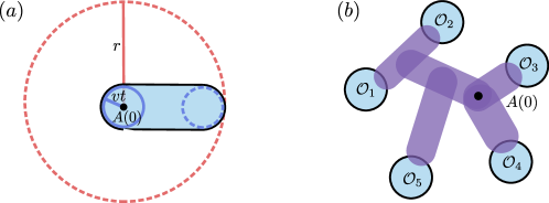
Figure 1: (a) The dominant contribution to the growth of an operator outside of the Lieb-Robinson light cone. Traditional Lieb-Robinson bounds suggest that the fraction of $A(t)$ acting on the red dotted circle to be suppressed by $\exp[-\mathrm{O}(r)]$. We show that it is suppressed by $\exp[-\mathrm{O}(r^{d})]$, which highly favors operators with “noodle-shaped” support like the one shown in blue. (b) An illustration of why this problem is so difficult to approach with conventional techniques, which count the number of paths of subsets (illustrated in purple) that connect the support of $A(0)$ to the support of $\mathcal{O}_{1},\dots\mathcal{O}_{m}$. The combinatorics of counting branching paths that grow operators to have large support becomes difficult at higher orders. This makes the equivalence-class method a very valuable tool.

In $d>1$, we must be careful about predicting the scaling directly from the number of terms in the perturbative expansion (3). As depicted in Figure 1b, the number of ways that an operator can grow to fill a large volume is exponentially large in volume itself! As we Taylor expand $A_{x}(t)$ at higher orders $n$ in $t$, the larger support of $[H_{X_{n-1}},\cdots,[H_{X_{1}},A_{x}]]$ means that there are yet more terms in $H$ that may not commute with the nested commutator at the $n^{\text{th}}$ step. As is known Araki (1969); Avdoshkin and Dymarsky (2020), the growth in the number of possible terms is enough to break the convergence of the series. Therefore, if the weight of an operator that fills an entire volume truly does decay as $\exp[-R^{d}]$, we must find a careful way to re-sum this series.

Our main technical tool for this re-summation is the equivalence class formalism recently introduced in Ref. Chen and Lucas (2021). In Section 3.3, we illustrate the flexibility in choosing which paths to include in the bound, and in Section 4 we leverage this flexibility to introduce a reformulation of the problem (as illustrated in Figure 4) that allows us to separate out the direct paths connecting sites within a ball of radius $R$ to $x$. As a tool for probing the support of an operator, we use nested commutators. In Theorems 4.4 and 5.13 for local and quasilocal Hamiltonians respectively, we prove the following bound, shown here in schematic form:

$$\|[\mathcal{O}_{m},[\dots,[\mathcal{O}_{1},A(t)]]]\|\lesssim\exp(m\mu(vt-r))$$ (5)

where $\mu,v>0$ are constants, $\|\cdot\|$ refers to the operator norm, and the supports of $\mathcal{O}_{1},\dots,\mathcal{O}_{m}$ are separated pairwise by at least $r>vt$. Since the $\mathcal{O}_{j}$ are outside of each others’ Lieb-Robinson light cone, we expect to find a good bound on (5). Intuitively, the nested commutator is a probe of the support of $A(t)$ because the operators $\mathcal{O}_{1},\dots,\mathcal{O}_{m}$ supported on sets $S_{1},\dots,S_{m}$ may be chosen to capture the contribution of Pauli-strings in the expansion of $A(t)$ which act simultaneously on $S_{1},\dots,S_{m}$. In particular, we can fit $m\sim\left(R/vt\right)^{d}$ such operators inside of a ball of radius $R$, while ensuring that no light cones overlap. This suggests that for $R>vt$, the fraction of an operator that acts non-trivially on a finite fraction of sites within a ball of radius $R$ scales as

$$\lVert A(t)_{\text{acts on ball of radius $R$}}\rVert\lesssim\exp[-(R-vt)^{d}/(vt)^{d-1}].$$ (6)

We prove this directly in Corollaries 4.11 and 5.14. At a high level, it certainly would seem that (6) is a dramatic improvement over a conventional Lieb-Robinson bound. Rather than scaling with the diameter of the support, the suppression depends on the volume.

In some applications, the nested commutator itself already is an interesting object to bound, in which case (5) is satisfactory. However, for applications such as bounding the simulatability of quantum dynamics on classical computers, directly characterizing the re-summation of terms is crucial. We achieve this in Section 6, where we explicitly derive an improved estimate for the simulation complexity of local and quasilocal quantum systems. In Corollary 6.3, we prove that for a system on a $d$-dimensional square lattice, the classical computation resources $N$ required to simulate the dynamics with error $\varepsilon$ are bounded by

$$N\lesssim\exp\left[\mathrm{O}\left((1+v_{\rm LR}t)^{d-1}\left(v_{\rm LR}t+\log\frac{1}{\varepsilon}\right)\right)\right]$$ (7)

This exhibits polynomial scaling in $\frac{1}{\varepsilon}$, and we conjecture that this bound has the best possible scaling in both $\varepsilon$ and $t$. In particular, this result recovers the $\exp(\mathrm{O}((v_{\rm LR}t)^{d}))$ time-dependence that one would expect from a simulation with a strict lightcone, such as a random unitary circuit Nahum et al. (2018); von Keyserlingk et al. (2018) while maintaining the polynomial scaling in error tolerance $\varepsilon$ for a fixed time.

We additionally explore the applications of bounds such as (5) in condensed matter physics. More concretely, we study spontaneous $\mathbb{Z}_{2}$-symmetry-breaking phases of quantum matter. In Theorem. 7.1, we show that if states $\ket{\psi_{\pm}}$ are connected to GHZ states $\ket{\pm}$ (symmetric under the broken $\mathbb{Z}_{2}$ symmetry) through a finite-time evolution under a local or quasilocal symmetric Hamiltonian, then the energy splitting between these states is exponentially suppressed in system volume. In other words, in a ferromagnetic phase, the splitting between the lowest two energy levels in the system is exponentially small in the volume of the system, rather than just the linear system size. Furthermore, in Theorem. 7.2 we show the that the disorder parameter, defined as $\lim_{R\to\infty}\left\langle\prod_{i\in B_{R}}X_{i}\right\rangle$ where $B_{R}$ is a $d$-dimensional ball of radius $R$, decays exponentially with the volume of $B_{R}$. These results suggest a new diagnostic tool to distinguish quantum phases of matter, which we illustrate via a concrete example with Rokhsar-Kivelson-like states Rokhsar and Kivelson (1988); Ardonne et al. (2004); Castelnovo and Chamon (2008).

3 Mathematical preliminaries

The remainder of the paper will discuss the above results in a more formal way. We will first introduce our notation and review some key results and ideas from previous work on Lieb-Robinson bounds. We collect such results in this section.

3.1 Many-body quantum systems

To discuss locality in a many-body quantum system, it is often helpful to associate the quantum degrees of freedom (‘qudits’) to the vertices of a graph. We can imbue the problem with a notion of spatial locality by adding edges between these vertices, providing a notion of distance between distinct qubits. We will begin the formal discussion with problems where qudits only interact with their nearest-neighbors on the resulting graph (with generalizations to exponentially decaying interactions discussed in Section 5), and in this context it is often helpful to define a factor graph Chen and Lucas (2021):

Definition 3.1 (Factor Graph).

A factor graph $G=(V,E,F)$ is a bipartite graph in which each node in the node set $V$ is connected to the factor set $F$ with edges $E\subseteq V\times F$. We assume that $G$ is connected. If $(v,X)\in E$, we write $v\in X$: vertex $v\in V$ is connected to factor $X\in F$. The distance $\mathsf{d}(x,y)$ between $x,y\in V$ is defined as the smallest number of factors contained in a connected path from $x$ to $y$ in $G$. For subsets $R,S\subset V$, $\mathsf{d}(R,S):=\min_{x\in R,y\in S}\mathsf{d}(x,y)$.

Definition 3.2 ($d$-dimensional system).

Given a factor graph $(V,E,F)$, define the ball of radius $r$ around vertex $v\in V$ as

$$B_{r}(v):=\{u\in V:\mathsf{d}(u,v)\leq r\}.$$ (8)

We say that $(V,E,F)$ is d-dimensional if for all $v\in V$ and sufficiently large $r$, there exist O(1) constants $C_{1,2}$ and $C_{1,2}^{\prime}$ such that

$$C_{1}^{\prime}r^{d}\leq|B_{r}(v)| \leq C_{1}r^{d},$$ (9a)

$$C_{2}^{\prime}r^{d-1}\leq|B_{r}(v)|-|B_{r-1}(v)| \leq C_{2}r^{d-1}.$$ (9b)

Finite factor graphs represent a useful language to speak about many-body systems, as formalized in the definition below. We demonstrate all our results where $V$, $E$, and $F$ are finite sets, but our formalism naturally extends to the thermodynamic limit.

Definition 3.3 (Many-body Quantum System with Nearest-Neighbor Interactions).

Given a factor graph $G=(V,E,F)$, we define a many-body Hilbert space

$$\mathcal{H}=\bigotimes_{v\in V}\left(\mathbb{C}^{q}\right)_{v}=:\left(\mathbb{C}^{q}\right)^{\otimes V},$$ (10)

for some $q\in\mathbb{N}$. Here $\left(\mathbb{C}^{q}\right)_{v}$ reminds us that the $q$-dimensional Hilbert space is associated with a degree of freedom at vertex $v$. The Hamiltonian is a Hermitian operator

$$H=\sum_{X\in F}H_{X},$$ (11)

where $X$, considered as a subset of $V$, is the support of $H_{X}$. We say that $\mathcal{H},H$ defines a many-body system with few-body interactions if for all $X\in F$, $|X|\leq\Delta$ for some fixed $\mathrm{O}(1)$ constant $\Delta$.

Definition 3.4 (Vector space of operators).

The space of all linear operators acting on $\mathcal{H}$ forms a vector space $\mathcal{B}$. When we wish to emphasize this, we will write $A\in\mathcal{B}$ as $|A)$. There is a natural adjoint action of any $A\in\mathcal{B}$ on $\mathcal{B}$: $\mathrm{ad}_{A}|B)=|[A,B])$. We often use $A_{S}\in\mathcal{B}_{S}$ to denote that $A$ is supported within $S\subset V$.

We can express the time-evolution of an operator $\mathcal{O}$ in the Heisenberg picture using the notation above:

$$\derivative{t}|\mathcal{O}(t))=\mathrm{i}|[H,\mathcal{O}(t)]):=\mathcal{L}|\mathcal{O}(t))\ .$$ (12)

The formal solution to this equation for a time-independent $H$, and thus a time-independent $\mathcal{L}$, is $|\mathcal{O}(t))=\mathrm{e}^{t\mathcal{L}}|\mathcal{O})$. Since $H=\sum_{X\in F}H_{X}$, we can similarly associate a superoperator $\mathcal{L}_{X}:=\mathrm{i}\operatorname{ad}_{H_{X}}$ to each $H_{X}$ and, through the bilinearity of the commutator, write $\mathcal{L}=\sum_{X\in F}\mathcal{L}_{X}$. In this paper, we will in general (for notational convenience) restrict to the study of $t$-independent $H$. However, it appears straightforward to confirm that all of our main results also hold for time-dependent systems.

3.2 Equivalence class construction of Lieb-Robinson bounds

A typical Lieb-Robinson bound is stated as follows: Chen et al.(2023)(Anthony) Chen, Lucas, and Yin (Anthony)

Theorem 3.5 (Lieb-Robinson bound).

Given a Hamiltonian $H$ on factor graph $G=(V,F,E)$, there exist $\mathrm{O}(1)$ constants $C,\mu,v_{\rm LR}$ such that for any two single-site operators $A_{R,S}\in\mathcal{B}_{R,S}$ respectively, for subsets $R,S\subset V$,

$$\lVert[A_{R}(t),A_{S}]\rVert\leq C\min(|\partial R|,|\partial S|)\mathrm{e}^{\mu(vt-\mathsf{d}(R,S))}.$$ (13)

Here $\lVert\cdots\rVert$ denotes the operator norm (maximum singular value of its argument), and $|\partial R|$ denotes the size of the boundary of $R$, which is the number of vertices in $R$ that are distance 1 from a vertex not in $R$.

Despite its seemingly technical nature, this result has broad applications (see Chen et al.(2023)(Anthony) Chen, Lucas, and Yin (Anthony) for a recent review). Although the Lieb-Robinson bound (13) is over 50 years old Lieb and Robinson (1972), we will now focus on a much more recent Chen and Lucas (2021) “equivalence class formulation” of Lieb-Robinson bounds, which we find will elegantly address the central question in this paper. Here, we will review this equivalence class formulation with a focus on the high-level ideas; a formal proof of the results outlined below follows from the more general method we develop in the next section.

Given operators $A_{i}$ and $\mathcal{O}_{j}$ supported on sites $i$ and $j$ respectively, traditional Lieb-Robinson bounds deal with the commutator

$$C_{ij}(t)=\frac{1}{2}\left\|[\mathcal{O}_{j},A_{i}(t)]\right\|=\frac{1}{2}\left\|\operatorname{ad}_{O_{j}}|A_{i}(t))\right\|\$$ (14)

analogously to Theorem 3.5, using single sites rather than sets for simplicity. We first express $|A_{i}(t))$ as:

$$\operatorname{ad}_{\mathcal{O}_{j}}e^{t\mathcal{L}}|A_{i})=\sum_{n=0}^{\infty}\frac{t^{n}}{n!}\sum_{X_{1},\dots,X_{n}\in F}\operatorname{ad}_{\mathcal{O}_{j}}\mathcal{L}_{X_{n}}\dots\mathcal{L}_{X_{1}}|A_{i})\ .$$ (15)

Each term in the sum can be uniquely labeled by a sequence of factors $M=(X_{1},\dots,X_{n})$. These sequences correspond to graphs whose nodes are elements of $F$, where $X_{1},X_{2}$ are connected by an edge if they share at least one vertex. One can show Chen and Lucas (2021) that the graphs that contribute nonvanishingly are trees for which $X_{m}\cap X_{k}\neq\emptyset$ for some $k<m$ for each $m$, and $j\in X$ for some $X\in M$. Such sequences are termed causal trees. There is a unique non-self-intersecting path connecting any two vertices in a tree. Such paths are referred to as irreducible paths. They play a central role in this derivation of the Lieb-Robinson bound.

Then the non-vanishing terms in (15) can be re-summed. Indeed, the challenge in developing Lieb-Robinson bounds is understanding how to organize the residual terms in such a way that as many terms as possible can be bounded all at once. The strategy of Chen and Lucas (2021) is to group the sequences into equivalence classes, where two sequences are said to be equivalent if the irreducible path $\Gamma$ in the sequence from $i$ to $j$ is the same. We label this equivalence class by $[\Gamma]\in\mathcal{S}$, where $\mathcal{S}$ is the set of such equivalence classes.

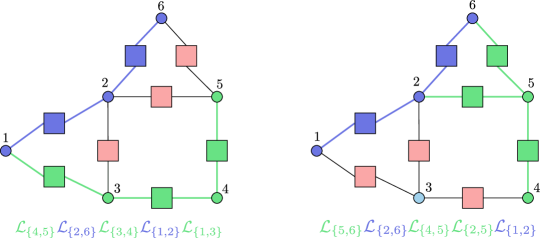
Figure 2: Example of two sequences of factors that appear in the expansion of the Liouvillian propagator which have the same irreducible path and thus belong to the same equivalence class. The boxes are factors and the circles are vertices. The irreducible path is shown in blue, while the irrelevant terms in the sequence are shown in green.

We can then regroup $\eqref{eq:resum}$ as

$$\sum_{n=0}^{\infty}\frac{t^{n}}{n!}\sum_{X_{1},\dots,X_{n}\in F}\prod_{i}\operatorname{ad}_{\mathcal{O}_{i}}\mathcal{L}_{X_{n}}\dots\mathcal{L}_{X_{1}}|\mathcal{\mathcal{missing}}O_{j})=\sum_{[\Gamma]\in S}\sum_{M\in[\Gamma]}\frac{t^{|M|}}{|M|!}\prod_{i}\operatorname{ad}_{\mathcal{O}_{i}}\mathcal{L}_{M_{|M|}}\dots\mathcal{L}_{M_{1}}|\mathcal{O}_{j})\ .$$ (16)

The terms in each equivalence class can then be re-summed to obtain the bound. The engine behind this re-summation is the generalized Schwinger-Karplus identity (Lemma 4.6). Applying this method to (16), the following Lieb-Robinson bound is obtained:

Theorem 3.6 (Theorem 3, Chen and Lucas (2021)).

If $\mathcal{O}_{j}\in\mathcal{B}_{j}$ and $A_{i}\in\mathcal{B}_{i}$ with $\|\mathcal{O}_{j}\|=\|A_{i}\|=1$, then

$$C_{ij}(t):=\frac{1}{2}\|\operatorname{ad}_{\mathcal{O}_{j}}e^{\mathcal{L}t}|A_{i})\|\leq\sum_{[\Gamma]\in\mathcal{S}}\frac{(2|t|)^{|\Gamma|}}{|\Gamma|!}w(\Gamma)$$ (17)

where $w(\Gamma)=\prod_{X\in\Gamma}\|H_{X}\|$ is the weight of $\Gamma$.

The equivalence classes are the set of non-self-crossing paths from $i\to j$, and counting arguments can then be used to simplify the form of this bound. The goal of our work is to then apply this method to iterated commutators.

3.3 Advantage over conventional Lieb-Robinson bounds

We remark briefly on the freedom in the choice of equivalence classes and how this freedom can be used to achieve tighter bounds in specific systems. Consider a chain consisting of four sites (see Fig. 3). The Hamiltonian is a sum of three terms $\{h_{1,2},h_{2,3},h_{3,4}\}$, with $\|h_{1,2}\|=\|h_{3,4}\|=h$ and $\|h_{2,3}\|=\varepsilon h$ with $\varepsilon\ll 1$. Let $A$ be an operator supported on site $1$ and $B$ supported on site $4$, both with unit norm. Using Theorem 3.6,

$$\|[A,B]\|\leq 2\sum_{[\Gamma]\in S_{ij}}\frac{(2|t|)^{l(\Gamma)}}{l(\Gamma)!}\prod_{X\in\Gamma}\|H_{X}\|=\frac{2\varepsilon(2h|t|)^{3}}{3!}$$ (18)

which follows because $\Gamma=(\{1,2\},\{2,3\},\{3,4\})$ is the only irreducible path connecting the two points.

The above does not take advantage of the fact that we know where the weak coupling is in the system. We could instead consider equivalence classes labeled by irreducible paths connecting $\{1,2\}$ with $\{3,4\}$, which in this simple example is trivially the factor $\mathcal{L}_{2,3}$. Similar ideas were described in Wang and Hazzard (2020); Baldwin et al. (2023). Applying the same theorem,

$$\|[A,B]\|\leq 4\varepsilon h|t|$$ (19)

If $\varepsilon\ll 1$, then this bound is nontrivial (smaller than 1) out to later times $t\lesssim\varepsilon^{-1}$, vs. $t\lesssim\varepsilon^{-1/3}$ for (18). The physical intuition for why this bound works is that we are effectively working in the interaction picture with $H_{0}=h_{12}+h_{34}$, rotating out the contribution of these terms to specifically target the weak link.

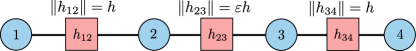
Figure 3: Example system showing the advantage to shortening the irreducible paths.

4 Nested commutator bounds

Having reviewed the standard single-commutator Lieb-Robinson bound, we now develop a formalism to obtain strong bounds on nested commutators. This section focuses on systems with only nearest-neighbor interactions on some interaction graph. The generalization to systems with exponential-tailed interactions (which is important for some of our applications) will be presented in Section 5.

4.1 Equivalence classes of causal trees

Let $H$ be a Hamiltonian associated to the factor graph $(F,E,V)$. Let $\mathcal{O}_{1},\dots,\mathcal{O}_{m}$ be operators with $\|\mathcal{O}_{i}\|=1$ and disjoint supports $S_{1},\dots,S_{m}$ respectively which are contained in regions $B_{1},\dots,B_{m}$. Consider an operator $A$ with $\|A\|=1$ whose support is a set $R$ contained within the complement of $B_{1},\dots,B_{m}$. We are interested in bounding the nested commutator

$$C_{\vec{S}}^{R}(t)=\sup_{\begin{subarray}{c}\mathcal{O}_{1},\dots\mathcal{O}_{m}\\ A\end{subarray}}\frac{1}{2^{m}}\|[\mathcal{O}_{m},[\dots,[\mathcal{O}_{1},A(t)]]\dots]\|$$ (20)

This is illustrated in Fig. 4.

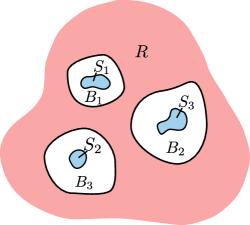
Figure 4: Illustration of the problem setup. This illustration is schematic, and the underlying vertex set is not shown. The region $R$ is depicted in red, and can be imagined as having infinite extent. The regions $S_{1},S_{2},S_{3}$ are depicted in blue, contained within the white regions $B_{1},B_{2},B_{3}$ which are disjoint from $R$. The shapes are arbitrary, but for particular applications we will find optimal choices for the shape of these regions.

As illustrated before, we can rewrite the time-evolved operator $A$ as

$$|A(t))=\mathrm{e}^{\mathcal{L}t}|A)=\sum_{M}\frac{t^{|M|}}{|M|!}\mathcal{L}_{M_{|M|}}\dots\mathcal{L}_{M_{1}}|A)$$ (21)

where again, $M=(M_{1},M_{2},\dots,M_{|M|})$ is a sequence of factors. The essence of our approach is to choose the appropriate equivalence classes to quantify the way that $A(t)$ “leaks” into the regions $B_{1},\dots,B_{m}$ over time. To accomplish this, we construct an algorithm to map each $M$ to a graph on subsets of $V$, slightly modifying the construction in Chen and Lucas (2021). The algorithm takes as input $S_{1},S_{2},\dots,S_{m}$, $R$, and $M$, where $M$ is a sequence of factors obtained from a term in the Liouville equation as described above, and outputs a forest (disjoint union of trees) $T(M)$. The algorithm proceeds as follows:

Algorithm 1 An algorithm for generating a causal forest

$T_{0}\leftarrow\{R\}$

$M_{0}\leftarrow R$

for $n\in\{1,\dots,|M|\}$ do

  $T_{n}\leftarrow T_{n-1}$

  if $\exists k<n$ s.t. $M_{n}\cap M_{k}\neq\emptyset$ then

   if $\neg\exists j<n$ s.t. $M_{n}\cap M_{j}=M_{n}$ then

     $k\leftarrow\min(\{k\text{ s.t. }M_{n}\cap M_{k}\neq\emptyset\})$

     $T_{n}\leftarrow T_{n-1}\cup(M_{n},(M_{k},M_{n}))$

   end if

   $T\leftarrow T_{n}$

   for $i$ s.t. $S_{i}\cap M_{n}\neq\emptyset$ and $S_{i}\not\in T_{n-1}$  do

     $T\leftarrow T\cup(M_{n},(S_{i},M_{n}))$

   end for

   $T_{n}\leftarrow T$

  else

   return $\emptyset$

  end if

end for

return $T_{|M|}$

The result of this algorithm is the forest $T(M)$.

Definition 4.1.

If $S_{1},\dots,S_{m}$ are nodes in the forest $T(M)$, then we call $T(M)$ a causal forest.

Proposition 4.2.

If $T(M)$ is not a causal forest, then $\prod_{i}\operatorname{ad}_{\mathcal{O}_{i}}\mathcal{L}_{M_{|M|}}\mathcal{L}_{M_{|M|-1}}\dots\mathcal{L}_{M_{1}}|A_{R})=0$.

Proof.

Let $S_{i}\notin T(M)$. By the design of the algorithm, this means that $M$ does not have an ordered subsequence of factors connecting $R$ to $S_{i}$. Since the factors correspond to the support of terms in the Hamiltonian, this means that $|B):=L_{M_{|M|}}\mathcal{L}_{M_{|M|-1}}\dots\mathcal{L}_{M_{1}}|A_{R})$ does not have support on $S_{i}$, so $\operatorname{ad}_{\mathcal{O}_{i}}|B)=0$. ∎

Definition 4.3.

If $T_{n}$ is a causal forest, then by construction, then each $S_{i}$ is contained in a tree rooted at $R$, so there is a unique path connecting it to $R$. This unique path $\Gamma_{i}=(X_{1},\dots,X_{l_{i}})\in F$, not including the endpoints at $S_{i}$ and $R$, is called the irreducible path to $S_{i}$. We will call $\mathcal{S}$ the set of equivalence classes of causal forests. An equivalence class of causal forests is defined by removing all the “reducible” terms (those not involved in $\Gamma_{i}$) from the sequence, arriving at a minimal sequence $\Lambda$ which will be called the irreducible skeleton.

An illustration of a causal forest constructed by the algorithm and the corresponding irreducible paths is depicted in Fig. 5.

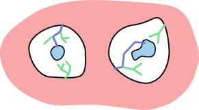
Figure 5: Example of a causal forest constructed by the algorithm. The red region again corresponds to $R$ and the two blue regions depict $S_{1},S_{2}$. The blue and green line segments represent factors in the sequence $M$. The blue segments participate in the irreducible paths, and so they form part of the corresponding irreducible skeleton, while the green ones are “reducible” terms. The ordering of the sequence is not depicted.

4.2 Bounds from irreducible paths

This section establishes the following bound on a nested commutator, which generalizes Theorem 3.6. The bound is is given by a product of the individual bounds from $R$ to each $S_{i}$:

Theorem 4.4.

Consider a local interaction defined by the factor graph $(V,E,F)$. Let $S_{1},\dots,S_{m}$ be sets contained in disjoint regions $B_{1},\dots,B_{m}$ separated by at least one on the subgraph of factors. Consider an operator $A$ with $\|A\|=1$ whose support is a set $R$ contained within the complement of $B_{1},\dots,B_{m}$. Let $\mathcal{O}_{1},\dots\mathcal{O}_{m}$ be operators also with norm $1$, where each $\mathcal{O}_{i}$ is supported within $S_{i}$. Then we have the following bound on the nested commutator:

$$\frac{1}{2^{m}}\|[\mathcal{O}_{m},[\dots,[\mathcal{O}_{1},A(t)]\dots]]\|\leq\prod_{i}\sum_{\Gamma\in\Gamma_{i}(R\to S_{i})}\frac{(2t)^{|\Gamma|}}{|\Gamma|!}w(\Gamma)$$ (22)

where $\Gamma_{i}(R\to S_{i})$ denotes the set of non-self-crossing paths within $B_{i}$ from $R$ to $S_{i}$ and $w(\Gamma)=\prod_{X\in\Gamma}\|H_{X}\|$ is the weight of the path $\Gamma$.

We begin by reorganizing the terms in (15) by equivalence class:

$$\prod_{i}\mathbb{\operatorname{ad}}_{\mathcal{O}_{i}}e^{\mathcal{L}t}|A_{R}) =\prod_{i}\operatorname{ad}_{\mathcal{O}_{i}}\sum_{[T]\in\mathcal{S}}\sum_{M:T(M)\in[T]}\frac{t^{|M|}}{|M|!}\mathcal{L}_{X_{|M|}}\dots\mathcal{L}_{X_{1}}|A_{R})$$ (23)

By definition each $T(M)\in[T]$ has the same set of irreducible paths $\{\Gamma_{i}\}$, so our goal is to rewrite the second sum in (23) by “factoring out” the contribution from the irreducible paths in the tree, then grouping together and safely re-summing the extraneous terms. This is accomplished in the following lemma:

Lemma 4.5.

Fix an equivalence class of causal forests $[T]$ with irreducible paths $\{\Gamma_{i}\}$ and irreducible skeleton $\Lambda$. Then

$$\prod_{i}\operatorname{ad}_{\mathcal{O}_{i}}\sum_{M:T(M)\in[T]}\frac{t^{|M|}}{|M|!}\mathcal{L}_{X_{n}}\dots\mathcal{L}_{X_{1}}|A_{R}) =\prod_{i}\operatorname{ad}_{\mathcal{O}_{i}}\sum_{m_{1},m_{2},\dots,m_{l}}\frac{t^{n}}{n!}(\mathcal{L}_{l})^{m_{l}}\mathcal{L}_{\Lambda_{l}}(\mathcal{L}_{l-1})^{m_{l-1}}\dots\mathcal{L}_{\Lambda_{1}}(\mathcal{L}_{0})^{m_{0}}|A_{R})$$ (24)

where $l:=|\Lambda|$ and $n:=l+\sum_{i}m_{i}$. We have defined

$$\mathcal{L}_{i}:=\sum_{X\cap V_{i}=\emptyset}\mathcal{L}_{X}$$ (25)

such that $V_{j}$ is the set of “disallowed” vertices: any factor that intersects $V_{j}$ would necessarily change the equivalence class of $T(M)$ if it was to appear in $M$ in between $\Lambda_{j}$ and $\Lambda_{j+1}$. We can break $V_{j}$ up into the terms disallowed by each path:

$$V_{j}=\bigcup_{i}U_{i,\beta_{i}(j)}$$ (26)

where $\beta_{i}(j)=\#\{k\leq j:i_{k}=i\}$ counts the number of terms in the sequence $\Lambda$ at or before position $j$ that belong to $\Gamma_{i}$. Let $l_{i}=|\Gamma_{i}|$. Then $U_{i,j}$ is explicitly defined as

$$U_{i,j}=\begin{cases}\bigcup_{m=\beta_{i}(j+2)}^{l_{i}}(\Gamma_{i})_{m}&j<l_{i}-1\\ S_{i}&j=l_{i}-1\end{cases}$$ (27)

Proof.

We follow Chen and Lucas (2021). First, we will show that every term on the right-hand side also appears in the summand on the left-hand side of (24). Fix an equivalence class $[T]$ with an irreducible skeleton $\Lambda=(\Lambda_{1},\dots,\Lambda_{l})$. Let $U_{i}:=\{\mathcal{L}_{X}:X\in F,\ X\cap V_{i}=\emptyset\}$, the set of terms allowed terms that could appear between $\Lambda_{i}$ and $\Lambda_{i+1}$, forming another factor sequence $M$ such that $[T(\Lambda)]=[T(M)]$. Then we can write

$$(\mathcal{L}_{l})^{m_{l}}\mathcal{L}_{\Lambda_{l}} (\mathcal{L}_{l-1})^{m_{l-1}}\dots\mathcal{L}_{\Lambda_{1}}(\mathcal{L}_{0})^{m_{0}}$$

$$=\quantity(\sum_{X_{1},\dots,X_{m_{l}}\in U_{l}}\mathcal{L}_{X_{1}}\dots\mathcal{L}_{X_{m_{l}}}^{l})\mathcal{L}_{\Lambda_{l}}\quantity(\sum_{X_{1},\dots,X_{m_{l-1}}\in U_{l-1}}\mathcal{L}_{X_{1}}\dots\mathcal{L}_{X_{m_{l-1}}})\dots\mathcal{L}_{\Lambda_{1}}\quantity(\sum_{X_{1},\dots,X_{m_{0}}\in U_{0}}\mathcal{L}_{X_{1}}\dots\mathcal{L}_{X_{m_{0}}})$$ (28)

Each term in parentheses is a sum over all possible sequences of allowed terms of length $m_{k}$, with repeated entries allowed. It is permissible for sequences which do not contribute to a causal tree to appear in the sum because the contribution of these terms must ultimately vanish. By construction, none of the terms $\mathcal{L}_{X_{k}}$ intersect any of the irreducible paths $\Gamma_{i}$ past $\beta_{i}(k)$, and so they may not create a path connecting $R$ to $S_{i}$. Therefore, any sequence appearing on the right hand side which has a non-vanishing contribution still corresponds to a tree $T(M)$ with the irreducible skeleton $\Lambda$. This shows that every non-vanishing term in the summand on the right-hand side corresponds to a causal forest in the equivalence class $[T(\Lambda)]$, and so it appears on the left-hand side.

For the other direction, every $T(M)\in[T(\Lambda)]$ may be constructed as $M_{l}\Lambda_{l}M_{l-1}\dots\Lambda_{1}M_{0}$, where $M_{l},\dots,M_{0}$ are arbitrary sequences of terms that form part of the causal forest but do not create additional paths between $R$ and $\{S_{1},\dots,S_{j}\}$, otherwise they would change the equivalence class of $T(M)$. As explained above, these are exactly the sequences that appear in the sum on the right-hand side. Furthermore, each term on the left and each term in the summand on then right correspond to a unique $M$. This establishes a bijection between the non-vanishing terms in the two sums, proving the result. ∎

In the next step, we can eliminate the contribution of extraneous “reducible” terms and include in the bound only contributions from the irreducible paths. The engine behind this re-exponentiation is the generalized Schwinger-Karplus identity:

Lemma 4.6 (Lemma 5, Chen and Lucas (2021)).

The following identity holds:

$$\sum_{\vec{m}=\vec{0}}^{\infty}\frac{t^{n}}{n!}\mathcal{F}_{l}^{m_{l}}A_{l}\dots\mathcal{F}_{1}^{m_{1}}A_{1}\mathcal{F}_{0}^{m_{0}}=\int\limits_{\Delta^{l}(t)}\mathrm{d}^{l}\vec{t}\mathrm{e}^{\mathcal{F}_{l}\Delta t_{l}}A_{l}\cdots\mathrm{e}^{\mathcal{F}_{1}\Delta t_{1}}A_{1}\mathrm{e}^{\mathcal{F}_{0}\Delta t_{0}}$$ (29)

where in the left-hand side we defined the term order $n:=l+\sum_{k=1}^{l}m_{k}$ and on the right-hand side, $\Delta^{l}(t)$ is the canonical $l-$simplex, and $\Delta t_{i}=t_{i+1}-t_{i}$, with $\Delta t_{l}:=t-t_{l}$ and $\Delta t_{0}:=t_{1}$.

Definition 4.7 ($n$-simplex).

We define the canonical $n-$simplex with side length $t$, denoted by $\Delta^{n}(t)$, as an $n-$dimensional shape bounded by $\{x_{1}<x_{2}<\dots<x_{n}<t\}$, which generalizes a triangle in 2D and a tetrahedron in 3D to $n$ dimensions. The volume of $\Delta^{n}(t)$ is given by

$$\operatorname{vol}{\Delta^{n}(t)}=\int\limits_{0}^{t}\mathrm{d}t_{1}\int\limits_{0}^{t_{1}}\mathrm{d}t_{2}\cdots\int\limits_{0}^{t_{n-1}}\mathrm{d}t_{n}=\frac{t^{n}}{n!}$$ (30)

Proof of Theorem 4.4.

By applying Lemma 4.5 and Lemma 4.6 to (24), we obtain

$$\left\|\frac{1}{2^{m}}\prod_{i}\operatorname{ad}_{\mathcal{O}_{i}}\mathrm{e}^{\mathcal{L}t}|A_{R})\right\| \leq\frac{1}{2^{m}}\sum_{[T]\in\mathcal{S}}\left\|\prod_{i}\operatorname{ad}_{\mathcal{O}_{i}}\sum_{T(M)\in[T]}\frac{t^{|M|}}{|M|!}\mathcal{L}_{X_{|M|}}\dots\mathcal{L}_{X_{1}}|A_{R})\right\|$$

$$\leq\sum_{\Lambda\in\mathcal{S}}\left\|\sum_{m_{1},m_{2},\dots,m_{q}}\frac{t^{n}}{n!}(\mathcal{L}_{l})^{m_{l}}\mathcal{L}_{\Lambda_{l}}(\mathcal{L}_{l-1})^{m_{l-1}}\dots\mathcal{L}_{\Lambda_{1}}(\mathcal{L}_{0})^{m_{0}}|A_{R})\right\|$$

$$\leq\sum_{\Lambda\in\mathcal{S}}\int\limits_{\Delta^{l}(t)}\mathrm{d}^{l}\vec{t}\left\|\exp(\mathcal{L}_{l}\Delta t_{l})\mathcal{L}_{\Lambda_{l}}\exp(\mathcal{L}_{l-1}\Delta t_{l-1})\dots\mathcal{L}_{\Lambda_{1}}\exp(\mathcal{L}_{0}\Delta t_{0})|A_{R})\right\|$$

$$\leq\sum_{\Lambda\in\mathcal{S}}\operatorname{vol}(\Delta^{l}(t))2^{l}\prod_{i=1}^{l}\|H_{\Lambda_{i}}\|$$ (31)

In the second line we use the fact that $\|\operatorname{ad}_{\mathcal{O}_{i}}\|_{op}\leq 2$ for $\|\mathcal{O}_{i}\|=1$, and in the fourth line we use the unitary invariance and submultiplicativity of the operator norm. Since $l=\sum_{j}|\Gamma_{j}|$ by definition, the canonical $n-$simplices have the property that

$$\operatorname{vol}(\Delta^{l}(t))=\frac{1}{l!}\prod_{j}|\Gamma_{j}|!\operatorname{vol}(\Delta^{|\Gamma_{j}|}(t))\ ,$$ (32)

so we can rewrite the right-hand side of (31) as

$$\sum_{\Lambda\in\mathcal{S}}\operatorname{vol}(\Delta^{l}(t))2^{l}\prod_{i=1}^{l}\|H_{\Lambda_{i}}\| =\sum_{\{\Gamma_{j}\}:(\Gamma_{1},\dots,\Gamma_{m})\in\mathcal{S}}\frac{1}{l!}\prod_{j=1}^{m}|\Gamma_{j}|!\operatorname{vol}(\Delta^{|\Gamma_{j}|}(t))2^{|\Gamma_{j}|}w(\Gamma_{j})$$ (33)

where the sum on the RHS is taken over all possible sets of irreducible paths $\{\Gamma_{j}\}$ such that the irreducible skeleton $\Lambda=(\Gamma_{1},\dots,\Gamma_{m})$ obtained from their concatenation belongs to $\mathcal{S}$. The summand does not depend on the ordering of the individual paths, only on the set of irreducible paths $\{\Gamma_{j}\}$ so we can reorganize the sum over sets of paths $\{\Gamma_{j}\}$:

$$\sum_{\Lambda\in\mathcal{S}}\operatorname{vol}(\Delta^{l}(t))2^{l}\prod_{i=1}^{l}\|H_{\Lambda_{i}}\| =\sum_{\{\Gamma_{i}\}}\frac{l!}{|\Gamma_{1}|!\dots|\Gamma_{m}|!}\frac{1}{l!}\prod_{i=1}^{m}|\Gamma_{i}|!\operatorname{vol}(\Delta^{|\Gamma_{i}|}(t))2^{|\Gamma_{i}|}w(\Gamma_{i})$$

$$=\sum_{\{\Gamma_{i}\}}\prod_{i=1}^{m}\operatorname{vol}(\Delta^{|\Gamma_{i}|}(t))2^{|\Gamma_{i}|}w(\Gamma_{i})=\prod_{i}\sum_{\Gamma\in\Gamma_{i}(R\to S_{i})}\frac{(2t)^{|\Gamma|}}{|\Gamma|!}w(\Gamma).$$ (34)

Hence we obtain (22). ∎

4.3 Combinatorial bounds

Although (22) is formally quite elegant, it is not necessarily always to work with. In this subsection, we will obtain more physically transparent nested commutator bounds by further simplifying (22). First, the nested commutator can be bounded using the equivalence class bounds on single commutators from Theorem 3.6:

Corollary 4.8 (Decoupling corollary).

Let $C_{ij}(t)$ be the bound on the single commutator in Theorem 3.6. Then

$$\frac{1}{2^{m}}\|[\mathcal{O}_{m},[\dots,[\mathcal{O}_{1},A(t)]\dots]]\|\leq\prod_{i}\sum_{\begin{subarray}{c}u\in\partial B_{i}\\ v\in\partial S_{i}\end{subarray}}C_{uv}(t)$$ (35)

This bound is not quite as tight as Theorem 4.4 because we now include paths that enter the region $R$. At short times, we find:

Corollary 4.9.

Suppose that $\|H_{X}\|\leq h$ for all $X$ that intersect with $B_{1},\dots,B_{m}$. Let $r_{i}:=\mathsf{d}(R,S_{i})$ and $\Delta$ be the maximum degree of the factor graph. If

$$|t|<\frac{\min_{i}(r_{i})}{2h\Delta},$$ (36)

then

$$C_{\vec{S}}^{R}\leq\prod_{i}|\partial B_{i}||\partial S_{i}|\quantity(\frac{2\mathrm{e}h|t|\Delta}{r_{i}})^{r_{i}}$$ (37)

Proof.

The number of distinct non-self-crossing paths of length $l$ from $u\in\partial B_{i}$ to $v_{i}$ must be smaller than $\Delta^{l}$. Given a ball $B_{i}$, the minimum length of path $\Gamma_{i}$ in a causal tree is $r_{i}:=d(R,v_{i})$. Therefore we have

$$\sum_{\Gamma_{i}(R\to v_{i})}\frac{(2t)^{|\Gamma|}}{|\Gamma|!}w(\Gamma)\leq\sum_{l=r_{i}}^{\operatorname{vol}(B_{i})}\frac{(2th\Delta)^{l}}{l!}$$ (38)

For any $\alpha>1$, $\alpha^{l-r_{i}}>1$ whenever $l>r_{i}$. We therefore find

$$\sum_{l=r_{i}}^{\operatorname{vol}(B_{i})}\frac{(2th\Delta)^{l}}{l!}\leq\inf_{\alpha>1}\sum_{l=0}^{\infty}\frac{(2th\Delta)^{l}}{l!}\alpha^{l-r_{i}}=\inf_{\alpha>1}\alpha^{-r_{i}}e^{2th\alpha\Delta}$$ (39)

If (36) holds, plugging in $\alpha=(2h\Delta t)^{-1}r_{i}>1$ into (39) gives

$$\inf_{\alpha>1}\alpha^{-r_{i}}\mathrm{e}^{2th\alpha\Delta}\leq\quantity(\frac{2\mathrm{e}h\Delta|t|}{r_{i}})^{r_{i}}$$ (40)

Inserting this bound into (22), we have

$$C_{\vec{S}}^{R}(t)\leq\prod_{i}|\partial B_{i}||\partial S_{i}|\quantity(\frac{2\mathrm{e}h\Delta|t|}{r_{i}})^{r_{i}}$$ (41)

as desired. ∎

Corollary 4.10.

Define

$$h_{ij}=\begin{cases}\sum_{X\in F:i,j\in X}\|H_{X}\|&i\neq j\\ 0&i=j\end{cases}$$ (42)

Then

$$C_{\vec{S}}^{R}\leq\prod_{i}\sum_{\begin{subarray}{c}u\in\partial B_{i}\\ v\in\partial S_{i}\end{subarray}}\exp(2h|t|)_{uv}$$ (43)

Proof.

The result follows immediately by combining Corollary 6 in Chen and Lucas (2021) with Cor. 4.8. ∎

Perhaps most importantly, we would like to have a bound that makes the volume-law decay of large nested commutators extremely transparent. This is accomplished by:

Corollary 4.11.

Let $B_{R}$ denote a metric ball of radius $R$. There exist constants $\gamma,c_{\rm{LR}}>0$ such that we can choose $v_{1},\dots,v_{m}\in B_{R}$ (where $m$ depends on $R$) for which

$$C_{v_{1},\dots,v_{m}}^{B_{R}^{c}}(t)\leq c_{\rm{LR}}\exp(-\gamma\frac{(R-v_{\rm LR}t)^{d}}{(v_{\rm LR}t)^{d-1}})$$ (44)

for any $v_{\rm LR}t>1$.

Proof.

We choose $S_{1},\dots,S_{m}$ to be vertices $v_{1},\dots,v_{m}$ and $B_{1},\dots,B_{m}$ to be metric balls $B_{i}=B_{\xi}(v_{i})$ of radius $\xi$ centered on these vertices. We will optimize $\xi$ to obtain (4.11). First suppose $d>1$. For a lattice in $d$ dimensions, there exists a constant $C_{1}$ such that $|\partial B_{\xi}|\leq(C_{1}\xi)^{d-1}$. Then directly applying Cor. 37, we have

$$C_{\vec{v}}^{R}(t)\leq\quantity[(C_{1}\xi)^{d-1}\quantity(\frac{v_{\rm LR}t}{\xi})^{\xi}]^{m}$$ (45)

Let $\xi=\alpha v_{\text{LR}}t$ for some $\alpha>1$. There exists a constant $C_{2}$ and, for any $\alpha$, a constant $K$, such that for all $v_{\rm LR}t>1$ and all $R>Kv_{\rm LR}t$, we can find $m$ distinct points $v_{1},\dots v_{m}$ in $B_{R}$ separated pairwise by more than $2\xi$, where $m>C_{2}\quantity(\frac{R}{\xi})^{d}$. The bound above may then be written as

$$C_{\vec{v}}^{B_{R}^{c}} \leq\quantity[\quantity(C_{1}\alpha v_{\rm LR}t)^{(d-1)\alpha^{-d}(v_{\rm LR}t)^{-1}}\quantity(\frac{1}{\alpha})^{\alpha^{1-d}}]^{C_{2}R^{d}(v_{\rm LR}t)^{1-d}}$$

$$\leq\quantity[\quantity(\frac{\mathrm{e}^{C_{1}(d-1)}}{\alpha})^{\alpha^{1-d}}]^{C_{2}R^{d}(v_{\rm LR}t)^{1-d}}$$ (46)

Then for any $\alpha>\exp(C_{1}(d-1))$, we have $(\mathrm{e}^{C_{1}(d-1)}\alpha^{-1})^{\alpha^{d-1}}:=\mathrm{e}^{-\beta}<1$. Plugging this in gives us

$$C_{\vec{v}}^{D^{c}}(t)\leq\exp(-\beta C_{2}R^{d}/(v_{\rm LR}t)^{d-1})$$ (47)

Additionally, $\beta$ achieves a maximum at $\alpha=\exp(C_{1}(d-1)+\frac{1}{d-1})>1$ of $\beta=\exp(-C_{1}(d-1)^{2}-1)/(d-1)$. This holds for $R>Kv_{\rm LR}t$, but we would like a bound that holds for all $R>v_{\rm LR}t$. If $\frac{R}{v_{\rm LR}t}<K$, then we can apply the traditional Lieb-Robinson bound (Thm. 3.5). Choosing $v_{1}$ at the center of $B_{R}$, we have

$$C_{\vec{v}}^{B_{R}^{c}}\leq\frac{1}{2}\|[\mathcal{O}_{v_{1}},A(t)]\|\leq c_{\text{LR}}\mathrm{e}^{\mu(v_{\rm LR}t-R)}$$ (48)

Let $C_{2}^{\prime}:=\beta C_{2}$, and for simplicity assume that $c_{\text{LR}}\geq 1$. For any $\lambda\leq 1$, we clearly have

$$\exp(-C_{2}^{\prime}R^{d}/(v_{\rm LR}t)^{d-1})\leq c_{\text{LR}}\exp(-C_{2}^{\prime}\lambda(R-v_{\rm LR}t)^{d}/(v_{\rm LR}t)^{d-1})$$ (49)

Then we find

$$e^{\mu(v_{\rm LR}t-R)}\leq\exp(-C_{2}^{\prime}\lambda(R-v_{\rm LR}t)^{d}/(v_{\rm LR}t)^{d-1})$$ (50)

when $\lambda\leq\frac{\mu}{C_{2}^{\prime}(\frac{R}{v_{\rm LR}t}-1)^{d-1}}$. If $1<\frac{R}{v_{\rm LR}t}<K$, then $\lambda=\min(\frac{\mu}{C_{2}^{\prime}(K-1)^{d-1}},1)<\frac{\mu}{C_{2}^{\prime}(\frac{R}{v_{\rm LR}t}-1)^{d-1}}$, so for all $\frac{R}{v_{\rm LR}t}>1$, we have

$$C_{\vec{v}}^{B_{R}^{c}}(t)\leq\exp(-\lambda C_{2}^{\prime}(R-v_{\rm LR}t)^{d}/(v_{\rm LR}t)^{d-1}).$$ (51)

This completes the proof. ∎

5 Hamiltonians with exponential tails

For some of our applications, it is important to extend our bounds to Hamiltonians with exponentially decaying interactions. The main issue is that we are no longer able to write each causal tree as a disjoint union of irreducible paths between the region $R$ and each $S_{i}$. In this section, we will describe how to overcome this difficulty when the Hamiltonian has exponential tails.

5.1 Review of Lieb-Robinson bounds for quasilocal Hamiltonians

Let $G=(V,E)$ be a graph with finite degree $\Delta$. In this section, unlike in the previous sections, we will use the distance $\mathsf{d}(x,y)$ to refer to the geodesic distance provided by the underlying graph $G$.

Definition 5.1.

We say a Hamiltonian $H$ is quasilocal if

$$H=\sum_{S\subseteq V}H_{S}\text{ such that $S$ is connected and }\|H_{S}\|\leq h\mathrm{e}^{-\kappa|S|}$$ (52)

for some constants $h$ and $\kappa$. A subset of the graph is connected if for each $u\in S$ there is some $v\in S$ such that $\mathsf{d}(u,v)=1$. $H_{S}$ does not need to act non-trivially on every site in $S$, but the decomposition (52) may only exist if most terms in $H$ are associated with the smallest possible set $S$. In this paper, we will for convenience restrict to

$$\kappa>1+\log\Delta.$$ (53)

Note that a more standard definition of quasilocal is (56); however, we will see that (52) is necessary for our main result in Theorem 5.13.

Proposition 5.2 (Theorem 3.7 in Chen et al.(2023)(Anthony) Chen, Lucas, and Yin (Anthony)).

Let $H$ be quasilocal. Suppose that $O$ is supported on a set $S\subset B$ and $A$ is supported on a set $R$ which is disjoint from but adjacent to $B$ as in Fig. 4. Then there exists constants $c_{\rm LR},\mu,v_{\rm LR}$ determined by $h,\kappa,\Delta$ such that

$$\frac{1}{2}\|[O,A(t)]\|\leq c_{\rm LR}|\partial B||\partial S|\mathrm{e}^{-\mu\mathsf{d}(R,S)}\left(\mathrm{e}^{\mu v_{\rm LR}t}-1\right)$$ (54)

In the case of strictly local Hamiltonians, a path needed a minimum length, measured on the factor graph, to couple two regions. Since we can no longer do this for quasilocal Hamiltonians, we have to use a different strategy, which we accomplish with the following two results:

Proposition 5.3 (Adapted from Haah et al. (2024)).

Given a vertex $u\in V$ on a graph of maximal degree $\Delta$, there are at most $(\Delta\mathrm{e})^{m}$ connected subsets $S$ with $u\in S$ and $|S|=m$. Furthermore, all these connected clusters of size $m$ can be enumerated classically in runtime $m\Delta(\Delta\mathrm{e})^{m}$.

This is obtained directly by Proposition 4.6 and Section 4.3 in Haah et al. (2024).

Lemma 5.4.

Let $u,v\in V$ be arbitrary. Then for any $\alpha>0$ there exists constants $\mu$, $h^{\prime}$ such that the following holds:

$$\sum_{X\ni u,v}\|H_{X}\|\leq\frac{h^{\prime}\mathrm{e}^{-\mu\mathsf{d}(u,v)}}{\mathsf{d}(u,v)^{\alpha}}$$ (55)

Proof.

We begin by overbounding the sum with every set which includes $u$ and has at least $\mathsf{d}(u,v)$ members, as required of a connected set containing both $u$ and $v$:

$$\sum_{X\ni u,v}\|H_{X}\|\leq\sum_{m\geq\mathsf{d}(u,v)}\sum_{\begin{subarray}{c}X\ni u\\ |X|=m\end{subarray}}\|H_{X}\|\leq h\sum_{m\geq\mathsf{d}(u,v)}(\mathrm{e}\Delta)^{m}\mathrm{e}^{-\kappa m}=\frac{h\mathrm{e}^{-(\kappa+1+\log(\Delta))\mathsf{d}(u,v)}}{1-\Delta\mathrm{e}^{-\kappa+1}}=:C\mathrm{e}^{-\mu^{\prime}\mathsf{d}(u,v)}$$ (56)

We have bounded the number of connected subsets $X$ containing $u$ of size $m$ with $(\mathrm{e}\Delta)^{m}$ by Proposition 5.3. Then the result is a geometric series, which converges due to (53). Now let $\alpha>0$. Since an exponential decays much more rapidly than a power-law, we can find $\mu$ dependent on $\alpha$ such that

$$C\mathrm{e}^{-\mu^{\prime}\mathsf{d}(u,v)}\leq h^{\prime}\frac{\mathrm{e}^{-\mu\mathsf{d}(u,v)}}{\mathsf{d}(u,v)^{\alpha}}$$ (57)

where $h^{\prime}$ is another constant dependent on $\alpha$ and $C$, but not dependent on $\mathsf{d}(u,v)$. This is the advertised result. ∎

The reason for requiring the power-law is that we need a way to iteratively apply this bound in order to constrain the weight of irreducible paths. This is captured in the following lemma:

Lemma 5.5.

For any $\alpha>d$, there exists a constant $K$ independent of $u,v$ such that

$$\sum_{k\neq u,v}\frac{\mathrm{e}^{-\mu\mathsf{d}(u,k)}}{\mathsf{d}(u,k)^{\alpha}}\frac{\mathrm{e}^{-\mu\mathsf{d}(k,v)}}{\mathsf{d}(k,v)^{\alpha}}\leq K\frac{\mathrm{e}^{-\mu\mathsf{d}(u,v)}}{\mathsf{d}(u,v)^{\alpha}}$$ (58)

This makes the function $G_{\alpha}(l):=\mathrm{e}^{-\mu l}l^{-\alpha}$ with $\alpha>d$ reproducing for the given lattice. This definition was introduced by Hastings in Def. 12 of Ref. Hastings (2010), where it was also pointed out that exponential decay alone is not reproducing, but can be made so by multiplication with a sufficiently fast power-law decay.

Proof of Proposition 5.2.

Applying the result from Theorem 3.6, the commutator is bounded by

$$\frac{1}{2}\|[O,A(t)]\|\leq\sum_{m=1}^{\infty}\frac{(2t)^{m}}{m!}\sum_{u\in\partial B,v\in\partial S}\sum_{\begin{subarray}{c}\Gamma(u\to v)\\ |\Gamma|=m\end{subarray}}w(\Gamma)$$ (59)

Now we need to bound the sum over weighted subsets. First fix some $u\in\partial B,v\in\partial S$. Then consider the irreducible path $\Gamma=(X_{1},X_{2},\dots,X_{m})$. We notice that the sets $X_{i}$ must form a connected path, i.e. $X_{k}\cap X_{k-1}\neq\emptyset$, so we can overbound the sum by summing over all such connected multisets. Furthermore, we can pick one point $v_{k}$ in each intersection $X_{k}\cap X_{k-1}$. Since this is true for each such connected multiset, we can further overbound the sum by considering all such sequences of vertices $\vec{v}=(u,v_{2},\dots,v_{m-1},v)$, where $v_{2},\dots,v_{m-1}$ are arbitrary, and sum over $\vec{X}=X_{1},\dots,X_{m}$ satisfying $v_{k}\in X_{k}\cap X_{k-1}$:

$$\sum_{\begin{subarray}{c}\Gamma(u\to v)\\ |\Gamma|=m\end{subarray}}w(\Gamma) \leq\sum_{v_{2},\dots,v_{m-1}}\sum_{X_{1}\ni u,v_{2}}\|H_{X_{1}}\|\dots\sum_{X_{m}\ni v_{m-1},v}\|H_{X_{m}}\|\leq h^{\prime m}\sum_{\vec{v}}\frac{\mathrm{e}^{-\mu\mathsf{d}(u,v_{2})}}{\mathsf{d}(u,v_{2})^{\alpha}}\dots\frac{\mathrm{e}^{-\mu\mathsf{d}(v_{m-1},v)}}{\mathsf{d}(v_{m-1},v)^{\alpha}}$$

$$\leq\frac{(h^{\prime}K)^{m}}{K}\frac{\mathrm{e}^{-\mu\mathsf{d}(u,v)}}{\mathsf{d}(u,v)^{\alpha}}$$ (60)

Thus we have the bound

$$\sum_{u\in\partial R,v\in\partial S}\sum_{\begin{subarray}{c}\Gamma(u\to v)\\ |\Gamma|=m\end{subarray}}w(\Gamma)\leq|\partial B||\partial S|\frac{(h^{\prime}K)^{m}}{K}\frac{\mathrm{e}^{-\mu\mathsf{d}(R,S)}}{\mathsf{d}(R,S)^{\alpha}}$$ (61)

Inserting this into (59), we find

$$C_{S}^{R}(t) \leq|\partial B||\partial S|\frac{\mathrm{e}^{-\mu\mathsf{d}(u,v)}}{K\mathsf{d}(u,v)^{\alpha}}\sum_{m=1}\frac{(2t)^{m}}{m!}(h^{\prime}K)^{m}$$

$$=|\partial B||\partial S|\frac{\mathrm{e}^{-\mu\mathsf{d}(u,v)}}{K\mathsf{d}(u,v)^{\alpha}}\left[\exp(2tKh^{\prime})-1\right]=c|\partial B||\partial S|\mathrm{e}^{-\mu\mathsf{d}(R,S)}(\mathrm{e}^{\mu v_{\rm LR}t}-1)$$ (62)

where we have introduced the constants $c=K^{-1}$ and $v_{\rm LR}=2Kh^{\prime}\mu^{-1}$. ∎

5.2 Extending to nested commutators: $m=2$ case

Now we can extend this result to nested commutators. For an illustrative example, we first consider the case where there are only two regions $B_{1},B_{2}$. In this section, we will illustrate the strategy for the general case by proving the following proposition:

Proposition 5.6.

For operators $\mathcal{O}_{1},\mathcal{O}_{2}$ supported on $S_{1},S_{2}$ respectively and $A$ supported in the complement of $B_{1}\cup B_{2}$, with $\mathcal{O}(1)$ constants $\mu,v_{\mathrm{LR}},h,h^{\prime}$ as defined in the previous section, we have

$$\frac{1}{4}\|[\mathcal{O}_{1},[\mathcal{O}_{2},A(t)]]\|\leq\mu v_{\rm LR}t(\mu v_{\rm LR}t+e^{-2(\mu\chi-\kappa)})\prod_{i=1,2}b|\partial B_{i}||\partial S_{i}|e^{\mu(v_{\rm LR}t-\mathsf{d}(S_{i},B_{i}))}$$ (63)

where $b:=\frac{h^{\prime}}{h}$ and $\chi\leq\mathsf{d}(B_{1},B_{2})/2$.

Before proceeding with the proof, we introduce a few definitions. The most important distinction with the single-region case in the previous section is that we now have factors which intersect both $B_{1}$ and $B_{2}$, so we can no longer immediately factor the paths into products within each $B_{i}$, as in Cor. 4.8. However, we can reduce to the decoupled case by sorting the equivalence classes in the following way:

Definition 5.7.

Let $[\Gamma]\in\mathcal{S}$ be an equivalence class with irreducible paths $\Gamma_{1}$ and $\Gamma_{2}$ connecting $S_{1}$ and $S_{2}$ to $R$ respectively. We will say that $\Gamma$ couples $B_{1}$ and $B_{2}$ if $\Gamma_{1}\cap\Gamma_{2}\neq\emptyset$.

Lemma 5.8.

If $\Gamma$ couples $B_{1}$ with $B_{2}$, then $\Gamma_{1}\cap\Gamma_{2}=X$, where $X$ is a factor. $X$ is the first element of both $\Gamma_{1}$ and $\Gamma_{2}$, and the only element of either path that intersects $R$.

Proof.

Let $X\in\Gamma_{1}\cap\Gamma_{2}$. The first element of an irreducible path is the only one that can intersect with $R$ by construction. Since $X$ is required to be connected, it must intersect with $R$. Therefore it must be the first element in the irreducible path $\Gamma_{1}$ and similarly for $\Gamma_{2}$. If $Y\in\Gamma_{1}\cap\Gamma_{2}$, then $X$ and $Y$ are both the first elements of both paths, so $X=Y$. ∎

This shows in particular that the irreducible skeletons in the coupled case can be reduced to the uncoupled case by removing the first term.

Proof of Prop. 5.6.

We will now divide the equivalence classes into uncoupled paths $\mathcal{S}_{d}$ and coupled paths $\mathcal{S}_{c}$. Then the commutator bound breaks into a sum:

$$\frac{1}{4}\|[\mathcal{O}_{1},[\mathcal{O}_{2},A(t)]]\|\leq\sum_{\Gamma\in\mathcal{S}_{d}}\frac{(2t)^{|\Gamma|}}{|\Gamma|!}w(\Gamma)+\sum_{\Gamma\in\mathcal{S}_{c}}\frac{(2t)^{|\Gamma|}}{|\Gamma|!}w(\Gamma)$$ (64)

By Cor. 4.8, we can bound the first term in this equation by

$$\sum_{\Gamma\in S_{d}}\frac{(2|t|)^{|\Gamma|}}{|\Gamma|!}w(\Gamma)\leq\prod_{i=1,2}c|\partial B_{i}||\partial S_{i}|\mathrm{e}^{-\mu\mathsf{d}(S_{i},B_{i})}(e^{\mu v_{\rm LR}t}-1)$$ (65)

We are left with just the second term to bound. For convenience, let

$$A(X\to Y;l):=\{(U_{1},\dots,U_{l}):U_{1}\cap X\neq\emptyset,U_{i}\cap U_{i-1}\neq\emptyset,U_{l}\cap Y\neq\emptyset\}$$ (66)

where $X,Y,U_{i}\subseteq V$. Although not all $X,Y\in F$, we will bound the sum by summing over all possible subsets. Accordingly, given $\vec{U}=(U_{1},\dots,U_{l})$ where $U_{i}\subseteq V$, we define

$$\prod_{i}\|H_{U_{i}}\|\delta_{U_{i}\in F}\leq\prod_{i}he^{-\kappa|U_{i}|}:=W(\vec{U})$$ (67)

Then we write as a shorthand for our bound on the single commutator

$$\sum_{\begin{subarray}{c}\Gamma(R\to S_{i})\\ |\Gamma|=l\end{subarray}}w(\Gamma)\leq\sum_{\vec{U}\in A(R\to S_{i};l)}W(\vec{U})\leq|\partial B_{i}||\partial S_{i}|\frac{(h^{\prime}K)^{l}}{K}\frac{\mathrm{e}^{-\mu\mathsf{d}(R,S_{i})}}{\mathsf{d}(R,S_{i})^{\alpha}}:=\frac{(h^{\prime}K)^{l}}{K}Q_{i}$$ (68)

Notice that in the first inequality, we have relaxed the bound by summing over non-irreducible (e.g. backtracking) paths $\vec{U}$ as well. By Proposition 5.8, we can break each path up into the first factor $X$ which couples the two balls, and sequences of factors $\vec{U}$, $\vec{V}$ which then couple $X$ to $S_{1}$ and $S_{2}$ respectively. Then we account for all the ways that the elements of $\vec{U}$, $\vec{V}$ can be permuted without changing the ordering, which contributes a factor of $\frac{(l_{1}+l_{2})!}{l_{1}!l_{2}!}$:

$$\sum_{\begin{subarray}{c}\Gamma\in\mathcal{S}_{c}\\ |\Gamma|=l\end{subarray}}w(\Gamma) \leq\sum_{l_{1}+l_{2}=l-1}\sum_{P:\begin{subarray}{c}P\cap B_{1}\neq\emptyset\\ P\cap B_{2}\neq\emptyset\end{subarray}}W(P)\sum_{\begin{subarray}{c}\vec{U}\in A(P\to S_{1};l_{1})\\ \vec{V}\in A(P\to S_{2};l_{2})\end{subarray}}\sum_{\text{ordering}\{U_{i}\}\cup\{V_{i}\}}W(\vec{U}\oplus\vec{V})$$

$$=\sum_{l_{1}+l_{2}=l-1}\frac{(l-1)!}{l_{1}!l_{2}!}\sum_{P:\begin{subarray}{c}P\cap B_{1}\neq\emptyset\\ P\cap B_{2}\neq\emptyset\end{subarray}}W(P)\sum_{\vec{U}\in A(P\to S_{1};l_{1})}W(\vec{U})\sum_{\vec{V}\in A(P\to S_{2};l_{2})}W(\vec{V})$$ (69)

where we used $\oplus$ to emphasize that $\vec{U}$ and $\vec{V}$ are concatenated together as sequences of sets. Now we recognize that if $P$ intersects both $B_{1}$ and $B_{2}$, then we can pick $u\in\partial B_{1}\cap P$ and $v\in\partial B_{2}\cap P$ and write $P=X\backslash\{u,v\}\sqcup Y\sqcup Z$, where $Y=P\cap B_{1}$, $Z=P\cap B_{2}$, and $X=P\cap R\cup\{u,v\}$. Then we can bound the sum over such $P$ by summing over $X,Y,Z$ satisfying $u,v\in X$, $u\in Y$, $v\in Z$. This is illustrated in Fig. 6.

Figure 6: Example of a long-range coupling term supported on $P=X\cup Y\cup Z$. Since $P$ must intersect the boundary of both $B_{1}$ and $B_{2}$ by the connectedness requirement, we pick two “anchor” points $u,v$ on the respective boundaries of these regions so that $u\in X,Y$ and $v\in X,Z$.

$$\sum_{l_{1}+l_{2}=l-1}\frac{(l-1)!}{l_{1}!l_{2}!}\sum_{P:\begin{subarray}{c}P\cap B_{1}\neq\emptyset\\ P\cap B_{2}\neq\emptyset\end{subarray}}W(P)\sum_{\vec{U}\in A(P\to S_{1};l_{1})}W(\vec{U})\sum_{\vec{V}\in A(P\to S_{2};l_{2})}W(\vec{V})$$

$$\leq\sum_{l_{1}+l_{2}=l-1}\frac{(l-1)!}{l_{1}!l_{2}!}\sum_{\begin{subarray}{c}u\in\partial B_{1}\\ v\in\partial B_{2}\end{subarray}}\sum_{X\ni u,v}\sum_{Y\cap X=u}\sum_{Z\cap X=v}W(X\cup Y\cup Z)\sum_{\vec{U}\in A(Y\to S_{1};l_{1})}W(\vec{U})\sum_{\vec{V}\in A(Z\to S_{2};l_{2})}W(\vec{V})$$

$$\leq\frac{\mathrm{e}^{2\kappa}}{h^{2}}\sum_{l_{1}+l_{2}=l-1}\frac{(l-1)!}{l_{1}!l_{2}!}\sum_{\begin{subarray}{c}u\in\partial B_{1}\\ v\in\partial B_{2}\end{subarray}}\sum_{X\ni u,v}W(X)\sum_{\vec{U}\in A(\{u\}\to S_{1};l_{1}+1)}W(\vec{U})\sum_{\vec{V}\in A(\{v\}\to S_{2};l_{2}+1)}W(\vec{V})$$ (70)

We have abused notation slightly in writing

$$W(X\cup Y\cup Z)=W(X\backslash\{u,v\}\sqcup Y\sqcup Z)=\frac{\text{e}^{2\kappa}}{h^{2}}W(X)W(Y)W(Z).$$ (71)

Applying Lem. 5.4, we bound $\sum_{X\ni u,v}w(X)\leq h^{\prime}\mathrm{e}^{-\mu\mathsf{d}(u,v)}\leq h^{\prime}\mathrm{e}^{-2\mu\chi}$. The remaining sums over paths are exactly the sums appearing in Lem. 5.5:

$$\frac{\mathrm{e}^{2\kappa}}{h^{2}}\sum_{l_{1}+l_{2}=l-1}\frac{(l-1)!}{l_{1}!l_{2}!}\sum_{\begin{subarray}{c}u\in\partial B_{1}\\ v\in\partial B_{2}\end{subarray}}\sum_{X\ni u,v}w(X)\sum_{\vec{U}\in A(\{u\}\to S_{1};l_{1}+1)}w(\vec{U})\sum_{\vec{V}\in A(\{v\}\to S_{2};l_{2}+1)}w(\vec{V})$$

$$\leq h^{\prime}\frac{1}{h^{2}}\mathrm{e}^{2\kappa}\mathrm{e}^{-2\mu\chi}\sum_{l_{1}+l_{2}=l-1}\frac{(l-1)!}{l_{1}!l_{2}!}\frac{(h^{\prime}K)^{l_{1}+1}}{K}Q_{1}\frac{(h^{\prime}K)^{l_{2}+1}}{K}Q_{2}$$

$$=h^{\prime}\quantity(\frac{h^{\prime}}{h})^{2}\mathrm{e}^{2\kappa}\mathrm{e}^{-2\mu\chi}Q_{1}Q_{2}\sum_{l_{1}+l_{2}=l-1}\frac{(l-1)!}{l_{1}!l_{2}!}(h^{\prime}K)^{l_{1}+l_{2}}$$ (72)

Now we can plug this bound into the LHS of (75):

$$\sum_{\Gamma\in\overline{\mathcal{S}}}\frac{(2t)^{|\Gamma|}}{|\Gamma|!}W(\Gamma)\leq h^{\prime}\sum_{l=1}^{\infty}\sum_{l_{1}+l_{2}=l-1}\frac{(2t)^{l}}{l!}\frac{(l-1)!}{l_{1}!l_{2}!}(h^{\prime}K)^{l_{1}}(h^{\prime}K)^{l_{2}}\prod_{i=1,2}b\mathrm{e}^{-\mu\chi+\kappa}Q_{i}$$ (73)

We can similarly rewrite this sum in terms of sums over $l_{1}$, $l_{2}$ alone

$$\sum_{l=1}^{\infty}\sum_{l_{1}+l_{2}=l-1}\frac{(2t)^{l}}{l!}\frac{(l-1)!}{l_{1}!l_{2}!}(h^{\prime}K)^{l_{1}}(h^{\prime}K)^{l_{2}} =2t\sum_{l_{1}=0}^{\infty}\sum_{l_{2}=0}^{\infty}\frac{(2h^{\prime}Kt)^{l_{1}}}{l_{1}!}\frac{(2h^{\prime}Kt)^{l_{2}}}{l_{2}!}\frac{1}{(l_{1}+l_{2}+1)}$$

$$\leq 2t\quantity(\sum_{l_{1}=0}^{\infty}\frac{(2h^{\prime}Kt)^{l_{1}}}{l_{1}!})\quantity(\sum_{l_{2}=0}^{\infty}\frac{(2h^{\prime}Kt)^{l_{2}}}{l_{2}!})$$

$$=2t\mathrm{e}^{2\mu v_{\rm LR}t}$$ (74)

where we used $v_{\mathrm{LR}}=\frac{2Kh^{\prime}}{\mu}$. Now with $K>1$, our bound simplifies to

$$\sum_{\Gamma\in\mathcal{S}_{c}}\frac{(2t)^{|\Gamma|}}{|\Gamma|!}w(\Gamma)\leq\mu v_{\rm LR}t\mathrm{e}^{-2\mu\chi+2\kappa}\prod_{i=1,2}b|\partial B_{i}||\partial S_{i}|\mathrm{e}^{\mu(v_{\rm LR}t-\mathsf{d}(S_{i},B_{i}))}$$ (75)

This gives a bound on the second term in (64). To obtain a simple expression for the sum, we observe that $\mathrm{e}^{t}-1\leq t\mathrm{e}^{t}$, which follows from a comparison of their Taylor series. Then we have $b>1$ because $h^{\prime}>h$, and $c=\frac{1}{K}<1$ by construction, so

$$\prod_{i=1,2}c|\partial B_{i}||\partial S_{i}|\mathrm{e}^{-\mu\mathsf{d}(S_{i},B_{i})}\left(\mathrm{e}^{\mu v_{\rm LR}t}-1\right)\leq\prod_{i=1,2}b|\partial B_{i}||\partial S_{i}|\mathrm{e}^{-\mu\mathsf{d}(S_{i},B_{i})}(\mu v_{\rm LR}t)e^{\mu v_{\rm LR}t}$$ (76)

Adding this to Eq. (75) gives the desired bound. ∎

We remark that since $\kappa\sim\mu$, if $\mu\chi>\kappa$ then as $\kappa\to\infty$ the factor $e^{2(\kappa-\mu\chi)}$ suppresses the contribution of the terms in $\mathcal{S}_{c}$, and we recover the product bound for the strictly local Hamiltonian.

5.3 Nested commutators: the general case

Now the goal is to generalize this proof to arbitrary $m$. Most of the manipulations are similar to those from the previous section. The problem now is that we need to account for long-range coupling between all possible subsets of the regions. If we were to naively sum the long-range couplings, the number of such subsets would grow much faster than the exponential suppression. In order to overcome this difficulty, we need to capture the fact that there are only very few small connected subsets coupling the regions, and the contribution of the large connected subsets are suppressed exponentially in the distance between these subsets. In order to formalize this notion, we note that in $d$ spatial dimensions, we can tile the plane with Euclidean boxes such that every box is adjacent to $3^{d}-1$ boxes. We will specialize to the case where each box contains at most one region $B_{1},\dots,B_{m}$, and the distance between $B_{i}$ and any other box is at least $\chi$. This is straightforwardly generalized to any way $\mathbb{R}^{d}$ can be broken into a course-grained lattice by tiling it with arbitrary shapes.

Definition 5.9.

If $[T]\in\mathcal{S}_{c}$ is an equivalence class of trees with irreducible paths $\Gamma_{1},\dots,\Gamma_{m}$ such that $\Gamma_{1}\cap\Gamma_{2}\cap\dots\cap\Gamma_{k}\neq\emptyset$ and $\Gamma_{i}\cap\Gamma_{j}=\emptyset$ for $i\leq k$ and $j>k$, then we will say that $[T]$ couples $B_{1},\dots,B_{k}$.

Proposition 5.10.

Let $T$ be a causal tree coupling $B_{1},\dots,B_{k}$. Let $\Gamma_{1},\dots,\Gamma_{k}$ be the irreducible paths coupling $S_{1},\dots,S_{k}$ to $R$. Then $\Gamma_{1}\cap\dots\cap\Gamma_{k}=X$, where $X$ intersects with $B_{1},\dots,B_{k}$, and $X$ is the first element of $\Gamma_{1},\dots,\Gamma_{k}$. Furthermore, all elements of $\Gamma_{i}\backslash\{X\}$ are contained within $B_{i}$ for each $i\leq k$.

Proof.

By the algorithm used to construct causal trees, the first element in each irreducible path is the only one to intersect $R$. Since $X$ must be connected and couples the regions, it must intersect with $R$. Therefore, removing $X$ from $\Gamma_{i}$ creates a path that lies entirely within $B_{i}$. ∎

Definition 5.11.

We call a connected set of boxes a cluster. For any $k\leq m$, a cluster containing $B_{1},\dots,B_{k}$ which has minimal volume is called a minimal cluster corresponding to $B_{1},\dots,B_{k}$. An example is illustrated in Fig. 7.

We will then proceed by induction on $m$. If a number of regions are coupled together as shown in Fig. 7 by a long-range term in a particular equivalence class, then by applying Cor. 4.8, we can factorize the system into two disjoint subsets of smaller size, which will establish the recursion.

Figure 7: Here $\mathbb{R}^{2}$ is covered with Euclidean boxes, and at most one region of interest $B_{i}$ is situated within each box with a distance at most $\chi$ from the edge of the box. $G$ is a subset of the regions representing the ways the region $16$ can coupled by a single term in a given irreducible path to the rest of the system, as shown in red. This coupling term is illustrated in blue. Since the coupling term is connected, it must pass through boxes that form a connected cluster, $G$ itself does not need to be connected. The green boxes show a minimal connected cluster containing $G$, which captures the exponential suppression of the terms coupling together the regions. We denote the number of green boxes by $M_{\mathrm{min}}(G)$. Our formalism accounts for terms like the one shown on the left that couple nearby balls as well as ones like the two shown on the right, which couple regions far away.

We will first derive the contribution from an equivalence class which couples $k$ regions using techniques from the previous section:

Lemma 5.12.

Suppose that $\mathcal{S}_{c}$ is the set of equivalence classes coupling $B_{1},B_{2},\dots,B_{k}$ with minimal cluster of order $M_{\mathrm{min}}$ and irreducible skeleton of length $l$. Then we can carry out the weighted sum over $\mathcal{S}_{c}$ with the following bound:

$$\sum_{l=1}^{\infty}\sum_{\begin{subarray}{c}\Lambda\in\mathcal{S}_{c}\\ |\Lambda|=l\end{subarray}}\frac{(2t)^{l}}{l!}w(\Lambda)\leq(\mu v_{\rm LR}t)\mathrm{e}^{-\mu\chi M_{\mathrm{min}}}\prod_{i}\mathrm{e}^{\kappa}b|\partial B_{i}||\partial S_{i}|\mathrm{e}^{\mu(v_{\rm LR}t-\mathsf{d}(S_{i},B_{i}))}$$ (77)

Proof.

Fix an equivalence class $\mathcal{S}_{c}$ that couples $B_{1},\dots,B_{k}$. As in the proof of Prop. 5.6, we can bound the sum by

$$\sum_{\begin{subarray}{c}\Lambda\in\mathcal{S}_{c}\\ |\Lambda|=l\end{subarray}}w(\Lambda) \leq\sum_{\sum_{k}l_{k}=l-1}\frac{(l-1)!}{l_{1}!\dots l_{k}!}\sum_{X\cap B_{1}\dots X\cap B_{k}\neq\emptyset}\|H_{X}\|\sum_{\vec{U}_{1}\in A(X\to S_{1};l_{1})}W(\vec{U}_{1})\dots\sum_{\vec{U}_{k}\in A(X\to S_{k};l_{k})}W(\vec{U}_{k})$$

$$\leq\sum_{\sum_{k}l_{k}=l-1}\frac{(l-1)!}{l_{1}!\dots l_{k}!}\sum_{u_{1}\in\partial B_{1}\dots u_{k}\in\partial B_{k}}\sum_{X\ni u_{1},\dots,u_{k}}W(X\backslash\{u_{1},\dots,u_{k}\})$$

$$\hskip 56.9055pt\times\sum_{\vec{U}_{1}\in A(\{u_{1}\}\to S_{1};l_{1})}W(\vec{U}_{1})\dots\sum_{\vec{U}_{k}\in A(\{u_{k}\}\to S_{k};l_{k})}W(\vec{U}_{k})$$

$$\leq h^{\prime}\quantity(\frac{h^{\prime}}{h})^{k}\mathrm{e}^{k\kappa}\mathrm{e}^{-\mu M_{\mathrm{min}}\chi}Q_{1}\dots Q_{k}\sum_{\sum_{i}l_{i}=l-1}\frac{(l-1)!}{l_{1}!\dots l_{k}!}(h^{\prime}K)^{l-1}$$ (78)

We have skipped a few steps because the manipulations are the same as Prop. 5.6. The significant difference is that each path needs to pass through a connected cluster, and the minimial cluster captures the number of boxes that it must either pass through or connect to the ball at the center. Therefore if the minimal cluster is of size $M_{\text{min}}$, the weight of this path is bounded by $W(X\backslash\{u_{1},\dots,u_{k}\})\leq h\mathrm{e}^{k\kappa}\mathrm{e}^{-\mu\kappa M_{\text{min}}}$, from which the bound on the summation of all possible subsets containing $u_{1}\in\partial B_{1},\dots,u_{k}\in\partial B_{k}$ follows as in Lem. 5.4. With this, we have

$$\sum_{l=1}^{\infty}\sum_{\begin{subarray}{c}\Lambda\in\mathcal{S}\\ |\Lambda|=l\end{subarray}}\frac{(2t)^{l}}{l!}w(\Lambda) \leq h^{\prime}\mathrm{e}^{-\mu\chi M_{\mathrm{min}}}\mathrm{e}^{k\kappa}\quantity(\prod_{i}b|\partial B_{i}||\partial S_{i}|e^{-\mu\mathsf{d}(S_{i},B_{i})})\sum_{l=1}^{\infty}\frac{(2t)^{l}}{l!}\quantity(\sum_{l_{1}+\dots+l_{k}=l-1}\frac{(l-1)!}{l_{1}!l_{2}!\dots l_{l}!}\prod_{i}(h^{\prime}K)^{l_{i}})$$ (79)

Then we can bound the compound sum with a product:

$$\sum_{l=1}^{\infty}\frac{(2t)^{l}}{l!}\sum_{l_{1}+\dots+l_{k}=l-1}\frac{(l-1)!}{l_{1}!l_{2}!\dots l_{l}!}\prod_{i}(h^{\prime}K)^{l_{i}} =2th^{\prime}\sum_{l_{1}+\dots+l_{k}=l-1}\frac{(2t)^{\sum_{i}l_{i}}}{l_{1}!\dots l_{k}!}\frac{1}{1+\sum_{i}l_{i}}\prod_{i}(h^{\prime}K)^{l_{i}}$$

$$\leq\mu v_{\rm LR}t\quantity(\sum_{l=0}^{\infty}\frac{(2h^{\prime}Kt)^{l}}{l!})^{k}$$

$$\leq\mu v_{\rm LR}t\mathrm{e}^{k\mu v_{\rm LR}t}$$ (80)

Inserting this into (79) gives the desired result. ∎

Theorem 5.13.

Consider a quasilocal interaction defined on a graph in $d$ dimensions. Suppose we tile the plane with Euclidean boxes, where each box has $3^{d}-1$ adjacent neighbors. Assume $B_{1},...,B_{m}$ are regions each contained within a separate box such that the distance between $B_{i}$ and any other box is at least $\chi$, where $\mu\chi>\max(\log(2)+d\log(3)+2,\kappa)$, and $S_{i}\subset B_{i}$. Then the following nested commutator bound holds:

$$\frac{1}{2^{m}}\|[\mathcal{O}_{m},[\dots,[\mathcal{O}_{1},A(t)]\dots]]\|\leq\mu vt(\mathrm{e}^{-\gamma+\kappa}+\mu vt)^{m-1}\prod_{i=1}^{m}|\partial B_{i}||\partial S_{i}|b\mathrm{e}^{\mu(v_{\rm LR}t-\mathsf{d}(S_{i},R))}$$ (81)

where $A$ is supported in $R$ which is the complimentary region to $\cup_{i}B_{i}$, $\mathcal{O}_{i}$ is supported within $S_{i}$, $\gamma=\mu\chi-\log(2\mathrm{e}3^{d})>1$, and $v=4\mathrm{e}3^{d}v_{\rm LR}$.

Proof.

Let $B_{1},\dots,B_{m}$ be defined as in the theorem statement. We will then induct on $m$. The base case is already proven in Sec. 5.1. We then consider an additional region $B_{m+1}$. We sort the equivalence classes by considering all the possible ways $B_{m+1}$ can be coupled to $B_{1},\dots,B_{m}$. For any $k\leq m$, let $\Lambda(\{i_{1},\dots,i_{k}\})$ denote the set of irreducible skeletons connecting $S_{i_{1}},\dots,S_{i_{k}}$ to $R$ and $\Gamma(\{i_{1},\dots,i_{k}\})$ denote the irreducible skeletons coupling $i_{1},\dots,i_{k}$. As we have shown in (4.2), we can bound the nested commutator with

$$\frac{1}{2^{m}}\|[\mathcal{O}_{m+1},[\dots,[\mathcal{O}_{1},A(t)]]\dots]\| \leq\sum_{\Lambda\in\Lambda(1,\dots,m)}\frac{(2|t|)^{|\Lambda|}}{|\Lambda|!}w(\Lambda)$$

$$\leq\sum_{\begin{subarray}{c}G\subseteq\{1,\dots,m,m+1\}\\ m+1\in G\end{subarray}}\quantity(\sum_{\Gamma\in\Gamma(G)}\frac{(2|t|)^{|\Gamma|}}{|\Gamma|!}w(\Gamma))\quantity(\sum_{\Lambda\in\Lambda(G^{c})}\frac{(2|t|)^{|\Lambda|}}{|\Lambda|!}w(\Lambda))$$ (82)

The decomposition above is illustrated in Fig. 7, with $G$ represented by the red circles (all connected to $B_{m+1}$) and $G^{c}$ being the yellow circles (not connected to $B_{m+1}$, not necessarily all connected to each other). Let $C(G):=\sum_{\Lambda\in\Lambda(G)}\frac{(2|t|)^{|\Lambda|}}{|\Lambda|!}w(\Lambda)$ with $C(\emptyset)=1$. Applying Lem. 5.12, we have a bound for the first term:

$$C(\{1,\dots,m,m+1\})\leq\sum_{\begin{subarray}{c}G\subseteq\{1,\dots,m,m+1\}\\ m+1\in G\end{subarray}}\mu v_{\rm LR}t\mathrm{e}^{-\mu\chi(M_{\mathrm{min}}(G)-1)}C(G^{c})\prod_{i\in G}|\partial B_{i}||\partial S_{i}|b\mathrm{e}^{\kappa(|G|-1)}\exp(\mu(v_{\rm LR}t-r_{i}))$$ (83)

where $r_{i}=\mathsf{d}(S_{i},R)$ for short. Since we assumed that $\mu\chi>\kappa$, and $|G|\leq M_{\mathrm{min}}(G)$ we relaxed $\mathrm{e}^{\kappa|G|}\mathrm{e}^{-\mu\chi M_{\mathrm{min}}(G)}$ to $\mathrm{e}^{\kappa(|G|-1)}\mathrm{e}^{-\mu\chi(M_{\mathrm{min}}(G)-1)}$. This choice greatly simplifies the induction because they make Lemma 5.12 consistent with the $m=1$ case that we proved in Sec. 5.1, thereby serving as a base case. Then we introduce $D(G)$ such that

$$C(G)=\prod_{i\in G}b|\partial B_{i}||\partial S_{i}|\exp(\mu(v_{\rm LR}t-r_{i}))D(G)$$ (84)

Then $D(G)$ satisfies the relationship

$$D(\{1,\dots,m,m+1\})\leq(\mu v_{\rm LR}t)\sum_{\begin{subarray}{c}G\subseteq\{1,\dots,m,m+1\}\\ m+1\in G\end{subarray}}\mathrm{e}^{(|G|-1)\kappa}\mathrm{e}^{-\mu\chi(M_{\mathrm{min}}(G)-1)}D(G^{c})$$ (85)

Now let

$$Q(k)=\sup_{\begin{subarray}{c}G\subseteq\{1,\dots,m,m+1\}\\ |G|=k\end{subarray}}D(G).$$ (86)

Notice that $Q(m+1)=D(\{1,\dots,m,m+1\})$ and $Q(0)=1$. This gives us the simpler but weaker bound

$$Q(m+1)\leq(\mu v_{\rm LR}t)\sum_{\begin{subarray}{c}G\subseteq\{1,\dots,m,m+1\}\\ m+1\in G\end{subarray}}\mathrm{e}^{(|G|-1)\kappa}\mathrm{e}^{-\mu\chi(M_{\mathrm{min}}(G)-1)}Q(m+1-|G|)$$ (87)

We can then bound the sum above by summing instead over connected clusters of boxes and then all possible subsets of those clusters:

$$\sum_{\begin{subarray}{c}G\subseteq\{1,\dots,m,m+1\}\\ G\ni m+1\end{subarray}} \mathrm{e}^{(|G|-1)\kappa}\mathrm{e}^{-\mu\chi(M_{\mathrm{min}}(G)-1)}Q(m+1-|G|)$$

$$=\mathrm{e}^{\mu\chi}\sum_{k=1}^{m+1}\mathrm{e}^{(k-1)\kappa}\sum_{M=k}^{\infty}\sum_{\begin{subarray}{c}\text{connected $X\ni m+1$}\\ |X|=M\end{subarray}}\sum_{\begin{subarray}{c}G\subseteq X\\ |G|=k\end{subarray}}\mathrm{e}^{-\mu\chi M}Q(m+1-k)$$

$$=\mathrm{e}^{\mu\chi}\sum_{k=1}^{m+1}\mathrm{e}^{(k-1)\kappa}\sum_{M=k}^{\infty}(\mathrm{e}3^{d})^{M}\binom{M}{k}\mathrm{e}^{-\mu\chi M}Q(m+1-k)$$

$$\leq\mathrm{e}^{\mu\chi}\sum_{k=1}^{m+1}\mathrm{e}^{(k-1)\kappa}\sum_{M=k}^{\infty}\mathrm{e}^{-M\gamma}Q(m+1-k)$$

$$\leq 4\mathrm{e}3^{d}\sum_{k=0}^{m}\mathrm{e}^{-k(\gamma-\kappa)}Q(m-k)$$ (88)

where we set $\gamma=\mu\chi-\log(2\mathrm{e}3^{d})$ and require that $\gamma>1$, which we can always ensure by choosing $\chi$ large enough. To obtain the third line, we used Prop. 5.3 to bound the number of clusters, and in the fourth line we bounded $\binom{M}{k}\leq 2^{M}$. With $Q(0)=1$ and $Q(1)\leq\mu v_{\rm LR}t\leq\mu vt$ already proven, for our inductive hypothesis we assume for $0<k\leq m$,

$$Q(k)\leq\mu vt(\mu vt+\mathrm{e}^{-(\gamma-\kappa)})^{k-1}$$ (89)

For convenience, let $t^{\prime}:=\mu vt$ and $a:=\mathrm{e}^{-(\gamma-\kappa)}$.

$$Q(m+1) \leq t^{\prime}a^{m}+t^{\prime}\sum_{k=1}^{m}a^{m-k}t^{\prime}(t^{\prime}+a)^{k-1}=t^{\prime}a^{m}+\sum_{k=1}^{m}a^{m-k}\sum_{j=0}^{k-1}\binom{k-1}{j}t^{\prime j+2}a^{k-1-j}$$

$$=t^{\prime}a^{m}+\sum_{j=0}^{m-1}a^{m-j-1}t^{\prime j+2}\sum_{k=j+1}^{m}\binom{k-1}{j}=t^{\prime}a^{m}+\sum_{j=0}^{m-1}a^{m-j-1}t^{\prime j+2}\binom{m}{m-j-1}$$

$$=t^{\prime}\sum_{j=0}^{m}a^{m-j}t^{\prime j}\binom{m}{m-j}=t^{\prime}(t^{\prime}+a)^{m}.$$ (90)

This completes the induction. We used the “hockey stick” relation $\sum_{m=k}^{n}\binom{m}{k}=\binom{n+1}{k+1}$ for the binomial coefficients. Unraveling the definition of $Q$,

$$\frac{1}{2^{m}}\|[\mathcal{O}_{m},[\dots,[\mathcal{O}_{1},A(t)]]\dots]\| \leq Q(m)\prod_{i}b|\partial B_{i}||\partial S_{i}|\exp(\mu(v_{\rm LR}t-r_{i}))$$

$$\leq\mu vt(\mu vt+\mathrm{e}^{-\gamma+\kappa})^{m-1}\prod_{i}b|\partial B_{i}||\partial S_{i}|\exp(\mu(v_{\rm LR}t-r_{i}))$$ (91)

This is the desired result. ∎

We remark on some of the properties of the above formula. Firstly, we see that the unlike the strictly local case, this bound is $\mathrm{\Theta}(t)$ for small $t$. This reflects the fact that there are now terms at first order that couple the $m$ regions to $R$. The term in the sum proportional to $t$ has a prefactor of $\mathrm{e}^{-(m-1)(\gamma-\kappa)}$. The $m-1$ instead of $m$ comes from the fact that we needed to relax the suppression in $\chi$ slightly to obtain this simple formula, but this reflects the fact that any term which directly couples all $m$ regions is exponentially suppressed in $m$. For example, expanding $Q(3)=t^{\prime 3}+2t^{\prime 2}a+a^{2}t^{\prime}$, we can identify the first term as decoupled, the second as originating from a coupling of two regions with the binomial coefficient counting the number of such couplings, and the last term representing a coupling between all three. Next, when $\mu\chi\gg\kappa,\log(2\mathrm{e}3^{d})$, the prefactor approaches $(\mu vt)^{m}$. This can be seen as the decoupled limit, and reflects the fact that one has to go to $m^{\text{th}}$ order to connect each $S_{i}$ to $R$, because irreducible skeletons $\Lambda$ with $|\Lambda|<m$ are exponentially suppressed. This also happens when we take $\kappa\to 0$, and since $\mu\sim\kappa$ the requirement that $\mu\chi>\kappa$ is well-behaved in this limit for fixed $\chi$. Lastly, we note that this bound is uniform in number of sites in the system $|V|$, which permits us to pass to the thermodynamic limit.

Corollary 5.14.

The conclusion of Cor. 4.11 holds for quasilocal interactions.

Proof.

First, consider the interaction graph embedded in $\mathbb{R}^{d}$. Let $\chi:=\max(\kappa,\log(2e^{2}3^{d}))/\mu$. There exists a constant $B$ such that for $\xi>1$, we can tile $\mathbb{R}^{d}$ with Euclidean boxes where each box contains a ball of radius $\xi+\chi$ and is contained within a ball of radius $B\xi$. Let $C_{1}$ be a constant such that $|\partial B_{\xi}|<(C_{1}\xi)^{d-1}$ for all $\xi>1$, and let $\xi:=\alpha vt$ for some $\alpha>1$. As in Cor. 4.11, there is a constant $C_{2}$ such that for each $\alpha>1$ we can find $K\gg 1$ such that for all $R>Kv_{\rm LR}t$ we can find $m>C_{2}\frac{R^{d}}{\xi^{d}}$ of these boxes lying entirely within $B_{R}$. Then from Thm. 5.13, we have

$$C_{\vec{v}}^{R}\leq\quantity((C_{1}\xi)^{d-1}e^{\mu(2vt-\xi)})^{C_{2}\frac{R^{d}}{\xi^{d}}}$$ (92)

where we used the fact that $\mu vt(\mu vt+e^{-\gamma+\kappa})^{m-1}\leq e^{m\mu vt}$. The bound above can be re-written as

$$\quantity((C_{1}\xi)^{d-1}e^{\mu(2vt-\xi)})^{C_{2}\frac{R^{d}}{\xi^{d}}} =\quantity((C_{1}\alpha vt)^{\frac{d-1}{\alpha vt}}\mathrm{e}^{\mu\frac{(2-\alpha)}{\alpha}})^{C_{2}\frac{R^{d}}{(\alpha vt)^{d-1}}}$$ (93)

Taking the logarithm of the term in parentheses,

$$\log((C_{1}\alpha vt)^{\frac{d-1}{\alpha vt}}\mathrm{e}^{\mu(2-\alpha)/\alpha})\leq\frac{1}{\alpha}\quantity[\frac{d-1}{\mathrm{e}}+(d-1)\log(C_{1}\alpha)+2\mu]-\mu:=-\beta$$ (94)

Since the first term on the right-hand side vanishes as $\alpha\to\infty$, it is clear that we can choose $\alpha$ large enough such that $\beta>\frac{\mu}{2}$. Thus the bound becomes

$$C_{\vec{v}}^{R}\leq\mathrm{e}^{-\frac{C_{2}\mu}{2\alpha^{d-1}}\frac{R^{d}}{(vt)^{d-1}}}$$ (95)

With this demonstrated for $R>Kv_{\rm LR}t$, the rest of the proof is the same as in Cor. 4.11, save for the fact that we must choose a smaller $\mu$ to achieve the same area prefactor in Prop. 5.2 as in Thm. 3.5. ∎

6 Accuracy of classical simulations of quantum dynamics

In random unitary circuits Nahum et al. (2018); von Keyserlingk et al. (2018), the dynamics are restricted by a light-cone with volume $\sim t^{d}$. The complexity of simulating these dynamics by truncating the operator outside of the light-cone is exactly bounded by $\exp(t^{d})$. This intuition breaks down for locally generated continuous-time evolution, where the light-cone is not sharp. As we discussed in the introduction, one then needs to specify an error tolerance $\varepsilon$ to which the simulation must be performed. Using classical Lieb-Robinson bounds, one expects that the truncation algorithm with tolerance $\varepsilon$ will produce a quasi-polynomial error growth $\sim\exp(\log(\varepsilon)^{d})$, which originates from failing to control the magnitude of the operator tails outside the light-cone. In Ref. Wild and Alhambra (2023), it was shown that for product initial states and strictly local interactions, a simulation algorithm based on truncating the support of an operator to a large subset achieves the optimal error scaling $\varepsilon^{-\exp(t)}$, which is polynomial in $\varepsilon$, but seemingly suboptimal in $t$ in finite dimensions. In this section, we will use the formalism developed above to revisit this question of bounding the difficulty of classically simulating quasilocal quantum dynamics.

6.1 Operator expansion with exponential-in-volume tails

In order to bound simulatability, we wish to have better control over the fraction of an operator which is supported on any large set $S$ containing $\gg(v_{\mathrm{LR}}t)^{d}$ vertices. We have already made progress along these lines. In Corollary 4.11 and Corollary 5.14, we made a weaker statement about the tail of an operator supported on vertices within a specific large set $S$. What remains is to show that, even though there are $\sim\exp(|S|)$ possible choices of connected sets with the volume of $S$ – a factor which is large enough to easily overwhelm the volume-law Lieb-Robinson bound in either corollary – the net contribution of all such large operators is still exponentially small in volume. This is achieved by the following theorem, where for technical convenience we restrict to dynamics on a square lattice:

Theorem 6.1.

Let $H$ be a quasilocal Hamiltonian on a $d$-dimensional square lattice $V$ of qudits, whose Lieb-Robinson bound is given by Proposition 5.2 with parameters $\mu,v_{\rm LR}$. Consider a local operator $A$ with $\norm{A}=1$ acting on $\mathrm{O}(1)$ nearby sites, which is evolved to $A(t)$ at time $t$ by $H$. It can be expanded to connected subsets $S$ that contain the support of $A$:

$$A(t)=\sum_{S\subset V}\widetilde{A}(S;t),$$ (96)

where $\widetilde{A}(S;t)$ is supported in $S$, such that all contributions from $|S|>M$ decay exponentially with the volume cutoff $M$: For any $M\geq 1$,

$$\widetilde{A}(t)=\sum_{S\subset V:|S|\leq M}\widetilde{A}(S;t),$$ (97)

approximates $A(t)$ with error

$$\norm{A(t)-\widetilde{A}(t)}\leq c_{d}\exp\quantity[4\mu v_{\rm LR}t-c_{d}^{\prime}\mu\frac{M}{(v_{\rm LR}t+c_{\rm box})^{d-1}}],$$ (98)

where $c_{d},c_{d}^{\prime},c_{\rm box}$ are constants determined by $d,\mu,v_{\rm LR}$.

Proof.

Similar to the previous section, we partition the lattice sites into non-overlapping boxes $V=b_{0}\sqcup b_{1}\sqcup\cdots$ where each box $b$ is a cube of length $r$ (thus containing $r^{d}$ sites), and the operator $A$ is contained in one box $b_{0}$. We choose $r$ to be

$$r=4(v_{\rm LR}t+c_{\rm box})>\max\quantity[d,\;\frac{45}{4\mu}3^{d}(\log 2+d\log 3)],$$ (99)

where the inequality holds by choosing a sufficiently large $\mathrm{O}(1)$ constant $c_{\rm box}$. The boxes can be viewed as vertices of a coarse-grained $d$-dimensional square lattice, and form a graph $G_{\rm b}=(V_{\rm b},E_{\rm b})$ where two boxes $b,b^{\prime}\in V_{\rm b}$ share an edge in $E_{\rm b}$ if and only if they are neighbors, because $\mathsf{d}(b,b^{\prime})\leq d$. Here $\mathsf{d}(\cdot,\cdot)$ is the distance function on the original lattice $V$. Note that here we do not work with factor graphs directly.

According to the Taylor expansion (15), we organize the time-evolved operator $A(t)=\mathrm{e}^{t\mathcal{L}}A$ by the boxes it touches (or has touched in the past by taking commutators with factors $X_{j}$ in the causal tree $(X_{1},\cdots,X_{n})$)

$$A(t)=\sum_{\text{connected }S_{\rm b}\subset V_{\rm b}:S_{\rm b}\ni b_{0}}A(S_{\rm b};t),$$ (100)

where

$$|A(S_{\rm b};t)):=\sum_{n=0}^{\infty}\frac{t^{n}}{n!}\sum_{X_{1},\dots,X_{n}\in F:\;\quantity(b\in S_{\rm b}\;\Leftrightarrow\;\exists X_{j}\text{ s.t. }X_{j}\cap b\neq\emptyset)}\mathcal{L}_{X_{n}}\dots\mathcal{L}_{X_{1}}|A).$$ (101)

In other words, we include the causal tree $(X_{1},\cdots,X_{n})$ in $A(S_{\rm b};t)$ if and only if the factors touch all boxes in $S_{\rm b}$ but no boxes in its complement $S_{\rm b}^{\rm c}$. Observe that we have restricted to subset of boxes $S_{\rm b}$ that are connected in $G_{\rm b}$ and contains $b_{0}$; otherwise $A(S_{\rm b};t)=0$ simply because the operator grows in a connected way. We call each $S_{\rm b}$ appearing in (100) as a connected cluster.

An equivalent way to express $A(S_{\rm b};t)$ is by induction: The starting point is

$$A(\{b_{0}\};t)=e^{t\mathcal{L}_{b_{0}}}A,$$ (102)

where $\mathcal{L}_{S}:=\sum_{X\in F:X\subset S}\mathcal{L}_{X}$. Then, given all $A(S_{\rm b};t)$ for $|S_{\rm b}|\leq m$, any $S^{\prime}_{\rm b}$ with size $|S^{\prime}_{\rm b}|=m+1$ is given by

$$A(S^{\prime}_{\rm b};t)=e^{t\mathcal{L}_{S^{\prime}_{\rm b}}}A-\sum_{S_{\rm b}\subsetneqq S^{\prime}_{\rm b}:\,S_{\rm b}\neq\emptyset}A(S_{\rm b};t),$$ (103)

where $\mathcal{L}_{S^{\prime}_{\rm b}}:=\mathcal{L}_{b_{0}\cup b_{1}\cup\cdots\cup b_{m}}$ for $S^{\prime}_{\rm b}=\{b_{0},b_{1},\cdots,b_{m}\}$. (103) holds because when Taylor-expanding $e^{t\mathcal{L}_{S^{\prime}_{\rm b}}}A$, any causal tree $(X_{1},\cdots,X_{n})$ that do not touch all boxes in $S^{\prime}_{\rm b}$ are canceled by a corresponding term in exactly one $A(S_{\rm b};t)$ in the second term of (103).

We adapt the multi-commutator bound Theorem 5.13 to show that $A(S_{\rm b};t)$ decays exponentially with $|S_{\rm b}|$. The proof of this result is delayed until Section 6.3.

Lemma 6.2.

There exist constants $c_{d}$ determined by $d$, and $c_{\rm box}$ determined by $d,\mu,v_{\rm LR}$, such that (99) holds, and for any connected cluster $S_{\rm b}$,

$$\norm{A(S_{\rm b};t)}\leq c_{d}\exp\quantity[-\mu(3^{-d}|S_{\rm b}|-1)r/5].$$ (104)

We then approximate $A(t)$ by an operator

$$\widetilde{A}(t)=\sum_{\text{connected cluster }S_{\rm b}:|S_{\rm b}|\leq m_{*}}A(S_{\rm b};t),$$ (105)

that truncates the sum over clusters in (100) at size $m_{*}$ (an integer). The truncation error is bounded by

$$\norm{A(t)-\widetilde{A}(t)} \leq\sum_{\text{connected cluster }S_{\rm b}:|S_{\rm b}|>m_{*}}\norm{A(S_{\rm b};t)}$$

$$\leq c_{d}\sum_{m>m_{*}}(3^{d}e)^{m}\exp\quantity[-\mu(3^{-d}m-1)r/5]$$

$$\leq c_{d}\exp\quantity[\frac{\mu r}{5}-m_{*}\quantity(3^{-d}\frac{\mu}{5}r-d\log 3)]\frac{1/2}{1-1/2}\leq c_{d}\exp\quantity[-\mu r(3^{-d-2}m_{*}-1)].$$ (106)

Here in the second line, we have applied Lemma 6.2 and Proposition 5.3 on the number of connected clusters $\leq(3^{d}e)^{m}$ of size $m$. In the last line, we have used

$$3^{-d}\frac{\mu}{5}r-d\log 3\geq\log 2,\;3^{-d-2}\mu r$$ (107)

from (99).

The theorem then follows by identifying $\widetilde{A}(S;t)$ with $A(S_{\rm b};t)$ where $S$ are the sites contained in $S_{\rm b}$. (98) comes from (6.1) with $M=m_{*}r^{d}$ and an updated constant $c_{d}$.

∎

6.2 Simulatability bound

According to the expansion obtained in Theorem 6.1, one can classically simulate $A(t)$ by its truncation $\widetilde{A}(t)$:

Corollary 6.3.

Let $H$ be a quasilocal Hamiltonian on a $d$-dimensional square lattice $V$ of qudits, whose Lieb-Robinson bound is given by Proposition 5.2 with parameters $c_{\rm LR},\mu,v_{\rm LR}$. Consider a local operator $A$ with $\norm{A}=1$ acting on $\mathrm{O}(1)$ nearby sites, and an initial state $\rho$ whose marginal $\rho_{S}$ on any connected set $S\subset V$ can be obtained classically with complexity $\exp[\mathrm{O}(|S|)]$. The expectation $\mathrm{Tr}[A(t)\rho]$ with any $t>0$ can be computed to error $\varepsilon$ with complexity

$$\exp[\mathrm{O}\quantity((1+v_{\rm LR}t)^{d-1}\quantity(v_{\rm LR}t+\log\frac{1}{\varepsilon}))].$$ (108)

Here the complexity assumption on the initial state applies to e.g. product states, thermal Gibbs states at high temperature Kliesch et al. (2014), and gapped ground states that are connected to solvable states by a gapped path of Hamiltonians Hastings and Wen (2005). The reason is that for those states, expectation values of local observables can be computed locally in an efficient way, so that the reduced density matrix $\rho_{S}$ can be obtained by state tomography with an extra $\exp[\mathrm{O}(|S|)]$ overhead. Note that our algorithm in the proof of Corollary 6.3 actually applies to more general initial states, which reduces the problem of computing local observables after time evolution to the problem of obtaining local marginals of the initial state.

(108) achieves a polynomial dependence of $1/\varepsilon$ even for $d>1$, which improves upon a quasi-polynomial bound $\exp[\mathrm{O}\quantity((v_{\rm LR}t+\log\frac{1}{\varepsilon})^{d})]$ from standard Lieb-Robinson bounds (see e.g. Proposition 4.4 in Chen et al.(2023)(Anthony) Chen, Lucas, and Yin (Anthony)). On the other hand, although a polynomial-in-$1/\varepsilon$ bound (Theorem 6 in Wild and Alhambra (2023)) has been obtained from cluster expansions in the restricted setting where $\rho$ is a product state, its complexity $\exp[\mathrm{O}\quantity(\mathrm{e}^{\mathrm{\Theta}(t)}\quantity(t+\log\frac{1}{\varepsilon}))]$ grows exponentially faster than (108) in terms of the $t$ dependence. The physical reason is that the cluster expansion techniques in Wild and Alhambra (2023) work for any bounded-degree graph. Our bound takes full advantage of the additional locality properties of finite-dimensional quantum systems. Our simulation complexity (108) thus rules out a proposed super-polynomial quantum advantage in analog quantum simulators Trivedi et al. (2024) while maintaining the correct scaling with $t$.

We argue that the bound (108) is tight with respect to the dependence on both $t$ and $1/\varepsilon$, because of the following. First, we argue that the $d=1$ case of (108) is tight because the Lieb-Robinson bound (13) can be (almost) saturated by a nearest-neighbor Hamiltonian Chen et al.(2023)(Anthony) Chen, Lucas, and Yin (Anthony), so the operator is effectively evolved in a truncated subsystem of $\mathrm{\Theta}(v_{\rm LR}t+\log\frac{1}{\varepsilon})$ qudits, whose simulation complexity is then exponential in the subsystem size and given in (108). Building on this 1d example, we expect the following time-dependent protocol $H(s)$ would saturate (108) for any constant dimension $d>1$ (note that Theorem 6.3 generalizes to time-dependent cases). Here time $s$ is backwards so that the operator $A$ first hits $H(0)$ instead of $H(t)$ in Heisenberg evolution. In the first half of the protocol $0<s<t/2$, $H(s)$ just evolves the initial local operator along a one-dimensional chain (e.g. $H(s)$ is a set of decoupled 1d Hamiltonians), so that there is a tail $A_{\rm tail}$ of the operator $A(t/2)$ that is supported in a chain of length $\sim v_{\rm LR}t+\log\frac{1}{\varepsilon}$ with

$$\norm{A_{\rm tail}}\sim\varepsilon.$$ (109)

Such a tail exists due to the tightness of Lieb-Robinson bound in 1d discussed above. The second half of the protocol $t/2<s<t$ then evolves in the horizontal directions of the original chain, which grows $A_{\rm tail}$ to a highly-entangled operator $A_{\rm tail}^{\prime}$ occupying a “cylinder” of height $\sim v_{\rm LR}t+\log\frac{1}{\varepsilon}$ and radius $\sim v_{\rm LR}t$. This second half can even be a quantum circuit with strict light cones. Since unitary evolution does not change operator norm (109) of this part of the operator $\norm{A_{\rm tail}^{\prime}}\sim\varepsilon$, one has to simulate dynamics in the whole cylinder to get precision $\varepsilon$, which requires complexity (108) that is an exponential of the cylinder volume.

Proof of Corollary 6.3.

In the proof of Theorem 6.1, we have expanded $A(t)$ into connected clusters $S_{\rm b}$. Choosing

$$m_{*}=\left\lfloor\frac{3^{d+2}}{\mu r}\log(\frac{2c_{d}}{\varepsilon})\right\rfloor+3^{d+2}+1,$$ (110)

the truncation error (6.1) leads to

$$\quantity|\mathrm{Tr}\quantity[\rho\quantity(A(t)-\widetilde{A}(t))]| \leq\norm{A(t)-\widetilde{A}(t)}\leq\frac{\varepsilon}{2}.$$ (111)

Therefore, to simulate $\mathrm{Tr}[\rho A(t)]$, it suffices to compute

$$\mathrm{Tr}[\rho\widetilde{A}(t)] =\sum_{\text{connected cluster }S_{\rm b}:|S_{\rm b}|\leq m_{*}}a(S_{\rm b}),$$ (112)

where

$$a(S_{\rm b}):=\mathrm{Tr}[\rho A(S_{\rm b};t)]=\mathrm{Tr}[\rho_{S_{\rm b}}A(S_{\rm b};t)],$$ (113)

only involves a marginal of the initial state $\rho_{S_{\rm b}}:=\rho_{b_{0}\cup b_{1}\cup\cdots\cup b_{m}}$ for $S_{\rm b}=\{b_{0},b_{1},\cdots,b_{m}\}$. According to (103),

$$a(S_{\rm b})=\widetilde{a}(S_{\rm b})-\sum_{S^{\prime}_{\rm b}\subsetneqq S_{\rm b}:\,S^{\prime}_{\rm b}\neq\emptyset}a(S^{\prime}_{\rm b}),$$ (114)

where

$$\widetilde{a}(S_{\rm b}):=\mathrm{Tr}[\rho_{S_{\rm b}}e^{t\mathcal{L}_{S_{\rm b}}}A]=\mathrm{Tr}[\rho_{S_{\rm b}}e^{\mathrm{i}tH_{S_{\rm b}}}Ae^{-\mathrm{i}tH_{S_{\rm b}}}].$$ (115)

The simulation algorithm then works as follows:

Algorithm 2 A classical simulation algorithm for $\mathrm{Tr}[\rho A(t)]$

Generate all connected clusters $S_{\rm b}\ni b_{0}$ with $|S_{\rm b}|\leq m_{*}$

Create array $a(S_{\rm b})\leftarrow 0$ for the generated clusters $\{S_{\rm b}\}$

for $m=1,2,\cdots,m_{*}$ do

  for all connected cluster $S_{\rm b}\ni b_{0}$ with $|S_{\rm b}|=m$ do

   Compute $\widetilde{a}(S_{\rm b})$ in (115) by exponentiating the matrix $H_{S_{\rm b}}$

   Update $a(S_{\rm b})$ by (114) using $\widetilde{a}(S_{\rm b})$ and the stored values for $a(S^{\prime}_{\rm b})$ where $|S^{\prime}_{\rm b}|<m$

  end for

end for

return $\sum_{S_{\rm b}}a(S_{\rm b})$

For each $\widetilde{a}(S_{\rm b})$, since it only involves a subsystem of $\leq m_{*}r^{d}$ qudits where the marginal $\rho_{S}$ is assumed to be computable in exponential time, $\widetilde{a}(S_{\rm b})$ can be computed accurately by

$$N=\exp[\mathrm{O}(m_{*}r^{d})]$$ (116)

resources. This dominates the complexity for $a(S_{\rm b})$, as the sum over $a(S^{\prime}_{\rm b})$ in (114) contains at most $\exp[\mathrm{O}(m_{*})]$ terms. Since there are at most $\exp[\mathrm{O}(m_{*})]$ clusters and they can be enumerated by a similar cost according to Proposition 5.3, the total complexity of the algorithm is still of the scaling (116), which becomes (108) by plugging in (99) and (110). The final error is bounded by $\varepsilon$ because the $m_{*}$ truncation error is bounded by $\varepsilon/2$ in (6.1), and the other operations like computing $\widetilde{a}(S_{\rm b})$ are essentially exact using resources above. ∎

6.3 Applying the multi-commutator bound: Proof of Lemma 6.2

Proof.

For $S_{\rm b}$ that only contains boxes $b_{0}$ or its nearest neighbors (there are $3^{d}-1$ of them), (104) holds by choosing a sufficiently large $c_{d}$ determined by $d$. The reason is that $\norm{A(\{b_{0}\};t)}\leq 1$ due to (102), and the other $\norm{A(S_{\rm b};t)}$ can be bounded by iterating (103): For example, let $b_{1}$ be one neighbor of $b_{0}$, then

$$\norm{A(\{b_{0},b_{1}\};t)}=\norm{e^{t\mathcal{L}_{\{b_{0},b_{1}\}}}A-A(\{b_{0}\};t)}\leq\norm{e^{t\mathcal{L}_{\{b_{0},b_{1}\}}}A}+\norm{A(\{b_{0}\};t)}\leq 1+1=2.$$ (117)

There are only finitely many $S_{\rm b}$ that only contains $b_{0}$ and its neighbors, so by a finite number of iteration they all satisfy $\norm{A(S_{\rm b};t)}\leq c_{d}$ for some constant $c_{d}$ determined by $d$, so that (104) is satisfied for them because the exponential factor is always $\leq 1$ for these $S_{\rm b}$ with $|S_{\rm b}|\leq 3^{d}$.

Beyond these finitely many connected clusters, any other $S_{\rm b}$ contains at least one box that are of distance $\geq r$ from the initial operator $A$. We can then find boxes $S_{1},S_{2},\cdots,S_{M}\in S_{\rm b}$ with $M\geq 1$ such that, each $S_{m}$ is surrounded by a larger box $B_{m}$ of side length $2(r-\chi)$ (where $\frac{r}{2}-\chi$ is an integer and $r,\chi\geq 1$ are chosen shortly) and the larger boxes $B_{1},\cdots,B_{M}$ have distance $\geq 2\chi$ from each other and from $b_{0}$. See Fig. 8 for an illustration. More precisely, because we have excluded the finitely many $S_{\rm b}$ in the neighborhood of $b_{0}$, we can always first find a $S_{1}\in S_{\rm b}$ whose larger box $B_{1}$ does not touch $b_{0}$. Then we try to find a $S_{2}\in S_{\rm b}$ that is not a neighboring box of $S_{1}$, and so on. We can always find such a set $S_{1},S_{2},\cdots,S_{M}\in S_{\rm b}$ containing at least

$$M\geq 3^{-d}|S_{\rm b}|-1,$$ (118)

boxes, because each $S_{m}$ only forbids its $3^{d}-1$ neighbors to be selected at the same time. Here we need the $-1$ in (118) to also avoid boxes neighboring $b_{0}$.

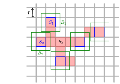
Figure 8: To apply the multi-commutator bound for a connected cluster $S_{\rm b}$ (red shaded region), we find boxes $S_{1},S_{2},\cdots,S_{M}\in S_{\rm b}$ (blue) that are well separated from each other and from the initial operator in $b_{0}$. We can always find $M=\mathrm{\Theta}(|S_{\rm b}|)$ number of them, which are surrounded by larger boxes $B_{1},\cdots$ that we use in the proof of the multi-commutator bound.

For a given $S_{\rm b}$, after finding these $M$ boxes $S_{m}$ together with their surrounding boxes $B_{m}$, we can then apply Theorem 5.13 to bound $\norm{A(S_{\rm b};t)}$. The reason is that although Theorem 5.13 is stated directly for the multi-commutator $C^{R}_{S_{1},\cdots,S_{M}}(t)$, its proof works by bounding individually each of the irreducible skeleton that contributes to $C^{R}_{S_{1},\cdots,S_{M}}(t)$. Here $\norm{A(S_{\rm b};t)}$ is also bounded by a sum over irreducible skeletons, with the only difference that here the causal forests in (100) corresponding to the irreducible skeletons are restricted to be contained in $S_{\rm b}$. In other words, $\norm{A(S_{\rm b};t)}$ is bounded by the bound on $C^{R}_{S_{1},\cdots,S_{M}}(t)$ if $H$ only contains terms supported inside $S_{\rm b}$; but this truncated $H$ is still a quasilocal Hamiltonian so we can just apply (81). Another small difference here is that $\{B_{m}\}$ do not lie in a square lattice. Theorem 5.13 generalizes to this case because its proof only uses the fact that the whole space can be tiled by $\{B_{m}\}$ and some other regions where the connectivity graph of the regions have bounded degree $\leq 3^{d}$; this property also holds here.

(81) thus implies

$$\norm{A(S_{\rm b};t)} \leq\quantity(c^{\prime}(t+1)\cdot r^{2(d-1)}\cdot e^{\mu(v_{\rm LR}t-r/2+\chi)})^{M}$$

$$\leq\quantity(c^{\prime\prime}r^{2d-1}\cdot e^{-\mu r/4})^{M}\leq\quantity(e^{-\mu r/5})^{M},$$ (119)

where $c^{\prime},c^{\prime\prime}$ are constants. Here in the first line, we have used $|\partial S_{i}|\leq|\partial B_{i}|=\mathrm{O}(r^{2})$ and chosen a sufficiently large constant $\chi$ independent of $t$ to get the factor $(t+1)$. In the second line of (119), we have used (99) with a sufficiently large constant $c_{\rm box}$, so that $t+1=\mathrm{O}(r)$ and $v_{\rm LR}t-r/2+\chi=-r/4-c_{\rm box}+\chi\leq-r/5-\mu^{-1}\log(c^{\prime\prime}r^{2d-1})$; this last condition is achievable because the function $f(r):=r/20-\mu^{-1}\log(c^{\prime\prime}r^{2d-1})$ is bounded from below. (104) follows by plugging (118) in (119). ∎

7 Spontaneous symmetry breaking phases of finite symmetries

We now turn to the second main application of our nested commutator bounds, and discuss the diagnosis of non-trivial phases of quantum matter. We focus on phases that exhibit spontaneous symmetry breaking (SSB) of finite symmetries. SSB can be detected by the presence of ground states with exponentially small energy splitting, along with order and disorder parameters computed in these nearly-degenerate states. For example, in the Ising ferromagnetic phase, there are two degenerate (in the thermodynamic limit) ground states $\ket{\psi_{\pm}}$ with eigenvalues $\pm 1$ under the global $\mathbb{Z}_{2}$ symmetry operator. These states are adiabatically connected to the $\pm$ GHZ states

$$\ket{\pm}=\frac{\ket{\mathbf{0}}\pm\ket{\mathbf{1}}}{\sqrt{2}}.$$ (120)

More concretely, it was shown in Ref. Hastings and Wen (2005) using Lieb-Robinson bounds that the splitting between the energies of $\ket{\psi_{\pm}}$ is at most exponentially small in the linear system size $L$:

$$\delta:=\left|\langle\psi_{+}|H|\psi_{+}\rangle-\langle\psi_{-}|H|\psi_{-}\rangle\right|\leq\mathrm{e}^{-\mathrm{O}(L)}.$$ (121)

However, deep in the ferromagnetic phase, one expects that adding a small transverse field $h\sum_{i}X_{i}$ would lead to $\delta\sim\mathrm{e}^{-\mathrm{O}(L^{d})}$, because the two ground states $\ket{\pm}$ are distinguished only by the global operator $\prod_{i}X_{i}$. Intuitively, this expectation is because it requires going to $\mathrm{O}(L^{d})$, not $\mathrm{O}(L)$, in perturbation theory, in order to connect $|\pm\rangle$ via perturbations.

Spontaneous symmetry breaking is also marked by a long-range order parameter $\lim_{|i-j|\to\infty}\bra{\psi}Z_{i}Z_{j}\ket{\psi}\sim\mathcal{O}(1)$ in states in the ground state subspace, as well as a quickly decaying disorder parameter $\lim_{R\to\infty}\bra{\psi}D_{R}\ket{\psi}$. Here, $d$ is the spatial dimension, and $D_{R}=\prod_{i\in B_{R}(v)}X_{i}$ is the global $\mathbb{Z}_{2}$ symmetry operator restricted to a $d$-dimensional ball of radius $R$ centered at any vertex $v$. Like with the splitting, conventional Lieb-Robinson bounds give a far looser bound, saying that $\lim_{R\to\infty}\langle\psi_{+}|D_{R}|\psi_{+}\rangle\lesssim\mathrm{e}^{-\mathrm{O}(R)}$ rather than the bound one might expect from perturbation theory: $\lim_{R\to\infty}\langle\psi_{+}|D_{R}|\psi_{+}\rangle\lesssim\mathrm{e}^{-\mathrm{O}(R^{d})}$. Indeed, this latter scaling is observed numerically Zhao et al. (2021).

7.1 Proofs of volume-law scaling

Using our nested commutator bound, we will confirm the intuition raised in the two arguments above. If states $\ket{\psi_{\pm}}$ are connected to the GHZ fixed point states $\ket{\pm}$ by finite time evolution generated by a quasilocal Hamiltonian (satisfying Definition 5.1), then the ground state splitting is in fact at most exponentially small in the volume of the system. Similarly, we will show that the disorder parameter is also at most exponentially small in the volume of $B_{\ell}(v)$. It was shown in Ref. Yin and Lucas (2024b) that in the vicinity of the ferromagnetic fixed point, such a quasilocal generator exists (the usual quasi-adiabatic generator Hastings (2004) that can be constructed within the entire ferromagnetic phase does not in general satisfy Definition 5.1). Therefore, at least for states in the vicinity of the ferromagnetic fixed point, our nested commutator results give bounds on the ground state energy splitting and disorder parameter that are much tighter than those given by the usual Lieb-Robinson bounds. It seems reasonable to conjecture that such a quasilocal generator might exist within the entire phase, not just in the vicinity of the fixed point. This would imply that these bounds hold within the entire ferromagnetic phase.

In the following, we will specialize to properties of the Ising ferromagnetic phase on a lattice in $d$ dimensions, with a constant finite density of sites with respect to the Euclidean distance, where each site hosts a qubit. However, our results are straightforward to generalize to spontaneous symmetry breaking phases of other finite symmetries, in systems with more general local Hilbert spaces. The following two theorems prove the two conjectures stated above, given the assumption of the exponential-in-volume-tailed quasi-adiabatic generator:

Theorem 7.1.

If $\ket{\psi_{\pm}}$ are ground states of a gapped, quasilocal Hamiltonian satisfying (5.1), that are connected to the $\pm$ GHZ states $\ket{\pm}$ defined in (120) in spatial dimension $d$ by finite-time evolution generated by a quasilocal Hamiltonian, then the splitting $\delta$ defined in (121) obeys

$$\delta\leq cL^{d}\mathrm{exp}\left(-\gamma\frac{(L-vt)^{d}}{(vt)^{d-1}}\right),$$ (122)

for $L\gg vt$, where $c,\gamma$ are $\mathcal{O}(1)$ constants, $L$ is the linear system size, and $v$ and $t$ are $\mathcal{O}(1)$ constants describing the finite time evolution and its quasilocal generator.

Theorem 7.2.

If $\ket{\psi}=U(t)\ket{\mathbf{0}}$ where $U(t)$ describes finite-time evolution in $d$ dimensions generated by a local, $\mathbb{Z}_{2}$ symmetric Hamiltonian, then the disorder parameter $\lim_{R\to\infty}\langle\psi|D_{R}|\psi\rangle$ for a $d$ dimensional ball of radius $R$ is upper bounded by

$$\lim_{R\to\infty}\bra{\psi}D_{R}\ket{\psi}\leq c_{\mathrm{LR}}\mathrm{exp}\left(-\gamma\frac{(R-vt)^{d}}{(vt)^{d-1}}\right),$$ (123)

where again $c_{\mathrm{LR}}$ and $\gamma$ are $\mathcal{O}(1)$ constants and $v,t$ describe the time evolution.

One subtlety about the above theorems is that in any given state $|t|$ may be very large, even $\mathcal{O}(\log L)$. Therefore, to probe the scaling of the disorder parameter and truly rule out the possibility that a state is connected to the ferromagnetic fixed point by finite (or $\mathcal{O}(\log L)$) time evolution generated by a quasilocal Hamiltonian, we need to compute expectation values of extensive operators and compare very small values (exponentially small in $L$ vs exponentially small $L^{d}$). In Sec. 7.2, we present an example of a state $|\psi(\beta)\rangle$ that fails to satisfy Theorem 7.2. However, due to the subtlety above, we can obtain another state $|\tilde{\psi}(\beta)\rangle$ whose overlap with $|\psi(\beta)\rangle$ goes to 1 in the thermodynamic limit, and does not violate Theorem 7.2. It is likely that $|\tilde{\psi}(\beta)\rangle$ can be connected to the ferromagnetic fixed point if we allow $|t|$ to be $\mathcal{O}(\log L)$. This point will be discussed more in depth in Ref. Sahay et al. (to appeara). However, for realistic systems where $t$ is an $\mathcal{O}(1)$ constant, the scaling of the disorder parameter provides a reliable diagnostic for the ferromagnetic phase.

To prove the above two theorems, we will make use of the following lemma. The rough idea of the lemma is that an expectation value of the form $\bra{\psi}D_{\mathrm{tot}}O\ket{\psi}$, where $D_{\mathrm{tot}}=\prod_{i}X_{i}$ is the global $\mathbb{Z}_{2}$ symmetry operator, can be written as the expectation value of a large nested commutator of various single site unitaries $Z_{i}$ with $O(t)$. Here, $\ket{\psi}=U(t)\ket{\mathbf{0}}$ where $U(t)$ is $\mathbb{Z}_{2}$ symmetric and $O(t)=U(t)^{\dagger}O(0)U(t)$. The polarized state is denoted by $\ket{\mathbf{0}}$, which is the unique eigenstate of every $Z_{i}$ operator with eigenvalue 1. This rewriting of $\langle\psi|D_{\mathrm{tot}}O|\psi\rangle$ will allow us to apply our nested commutator bound.

Lemma 7.3.

Let $O$ be an operator and let $|\psi\rangle=U(t)|0\rangle$. Then for any subset of sites $v_{1},\dots,v_{m}$, we have

$$\bra{\psi}D_{\mathrm{tot}}O\ket{\psi}=\frac{1}{2^{m}}\bra{\mathbf{0}}D_{\mathrm{tot}}[[\dots[O(t),Z_{v_{1}}],\dots Z_{v_{m-1}}],Z_{v_{m}}]\ket{\mathbf{0}}:=\frac{1}{2^{m}}\bra{\mathbf{0}}D_{\mathrm{tot}}[O(t),Z_{\vec{v}}]\ket{\mathbf{0}}.$$ (124)

Proof.

We use the following observations: (1) the evolution operator $U(t)$ commutes with $D_{\mathrm{tot}}$, (2) $\ket{\mathbf{0}}$ is an eigenstate of $Z_{v_{i}}$, and (3) $Z_{v_{i}}$ anticommutes with $D_{\mathrm{tot}}$. Putting these observations together, we get

$$\bra{\psi}D_{\mathrm{tot}}O\ket{\psi} =\bra{\mathbf{0}}D_{\mathrm{tot}}O(t)\ket{\mathbf{0}}$$

$$=\bra{\mathbf{0}}Z_{v_{1}}D_{\mathrm{tot}}O(t)\ket{\mathbf{0}}$$

$$=-\bra{\mathbf{0}}D_{\mathrm{tot}}Z_{v_{1}}O(t)\ket{\mathbf{0}}$$

$$=\bra{\mathbf{0}}D_{\mathrm{tot}}[O(t),Z_{v_{1}}]\ket{\mathbf{0}}-\bra{\psi}D_{\mathrm{tot}}O\ket{\psi}.$$ (125)

Rearranging the above gives $\bra{\psi}D_{\mathrm{tot}}O\ket{\psi}=\frac{1}{2}\bra{\mathbf{0}}D_{\mathrm{tot}}[O(t),Z_{v_{i}}]\ket{\mathbf{0}}$. This is the base case. Now we assume that (124) holds for a subset of sites $\vec{v}^{\prime}=(v_{1},\cdots,v_{m-1})$, and use the exact same reasoning to make the inductive step:

$$\bra{\psi}D_{\mathrm{tot}}O\ket{\psi} =\frac{1}{2^{m-1}}\bra{\mathbf{0}}D_{\mathrm{tot}}[O,Z_{\vec{v}^{\prime}}]\ket{\mathbf{0}}$$

$$=-\frac{1}{2^{m-1}}\bra{\mathbf{0}}D_{\mathrm{tot}}Z_{v_{m}}[O,Z_{\vec{v}^{\prime}}]\ket{\mathbf{0}}$$

$$=\frac{1}{2^{m-1}}\left(\bra{\mathbf{0}}D_{\mathrm{tot}}[[O,Z_{\vec{v}^{\prime}}],Z_{v_{m}}]\ket{\mathbf{0}}-\bra{\mathbf{0}}D_{\mathrm{tot}}[O,Z_{\vec{v}^{\prime}}]\ket{\mathbf{0}}\right)$$

$$=\frac{1}{2^{m}}\bra{\mathbf{0}}D_{\mathrm{tot}}[O,Z_{\vec{v}}]\ket{\mathbf{0}},$$ (126)

where $\vec{v}=(v_{1},\cdots,v_{m-1},v_{m})$ and we denote $[O,Z_{\vec{v}}]:=[[\dots[O,Z_{v_{1}}],\dots],Z_{v_{m}}]$. This completes the proof. ∎

With this technical lemma in hand, we now prove the theorems:

Proof of Theorem 7.1.

Using $\ket{\psi_{\pm}}=U(t)\ket{\pm}$, we obtain

$$\delta =|\bra{+}H(t)\ket{+}-\bra{-}H(t)\ket{-}|$$

$$=2\left|\mathrm{Re}\left\{\bra{\mathbf{1}}H(t)\ket{\mathbf{0}}\right\}\right|$$

$$=2\left|\mathrm{Re}\left\{\bra{\mathbf{0}}D_{\mathrm{tot}}H(t)\ket{\mathbf{0}}\right\}\right|$$

$$\leq 2\sum_{u\in V}\sum_{X\ni u}\left|\mathrm{Re}\left\{\bra{\mathbf{0}}D_{\mathrm{tot}}H_{X}(t)\ket{\mathbf{0}}\right\}\right|.$$ (127)

where in the last line, we decomposed the $H(t)$ into terms on connected clusters $X$ as in (5.1). Note that we did not need to assume that $U(t)$ is $\mathbb{Z}_{2}$ symmetric here because we did not need to apply the first step of (7.1).

If $H$ is strictly local, then we just have a sum over $u\in V$ and each of the terms above is of the form $\bra{\mathbf{0}}D_{\mathrm{tot}}O(t)\ket{\mathbf{0}}$, so we can apply Lemma 124 and then Theorem 5.13 to bound each term. Then Theorem 7.1 follows directly from Corollary 5.14. There is an overall factor of $L^{d}$ coming from the sum over $u\in V$.

If $H$ is quasilocal, then we divide the sum into clusters $X$ of size $|X|<\frac{L^{d}}{(B\xi)^{d-1}}$ and $|X|\geq\frac{L^{d}}{(B\xi)^{d-1}}$, where $B\xi$ is the linear size of the $m$ boxes that we divide the lattice into in Corollary 5.14, to fit in $m$ balls containing the operators $Z_{v_{1}},\dots Z_{v_{m}}$. Roughly speaking, for every $u\in V$, we will sum over the connected clusters $X$ containing $u$ (of which there are $\leq(\mathrm{e}\Delta)^{|X|}$ by Proposition 5.3) suppressed by their weight $h\mathrm{e}^{-\kappa|X|}$ and further suppressed by a nested commutator obtained by inserting as many balls as possible in a region of size $\sim L^{d}-|X|$. More precisely, the nested commutator can include all of the operators $Z_{v_{1}},\dots Z_{v_{m}}$ except for those in boxes that overlap with $X$. To accommodate for the worst-case scenario where the connected cluster $X$ forms a net along the edges of the boxes of linear size $B\xi$ (see the definitions in Corollary 5.14), to touch as many boxes as possible for smallest $|X|$, we use a region of size $L^{d}-(B\xi)^{d-1}|X|$ rather than $L^{d}-|X|$. Once $|X|\sim\frac{L^{d}}{(B\xi)^{d-1}}$, the worst-case scenario gives no further suppression from the nested commutators. Putting the above observations together, we get

$$\begin{split}\delta&\leq 2hL^{d}\left(\sum_{\begin{subarray}{c}X\ni u\\ |X|<L^{d}/(B\xi)^{d-1}\end{subarray}}(\mathrm{e}\Delta)^{|X|}\mathrm{e}^{-\kappa|X|}\mathrm{e}^{-\frac{C_{2}\mu}{2\alpha^{d-1}}\frac{L^{d}-(B\xi)^{d-1}|X|}{(vt)^{d-1}}}+\sum_{\begin{subarray}{c}X\ni u\\ |X|\geq L^{d}/(B\xi)^{d-1}\end{subarray}}(\mathrm{e}\Delta)^{|X|}\mathrm{e}^{-\kappa|X|}\right)\\ &\leq 2hL^{d}\left(\mathrm{e}^{-\frac{C_{2}\mu}{2\alpha^{d-1}}\frac{L^{d}}{(vt)^{d-1}}}\sum_{\begin{subarray}{c}X\ni u\\ |X|<L^{d}/(B\xi)^{d-1}\end{subarray}}\left(\Delta\mathrm{e}^{1-\kappa}\mathrm{e}^{\frac{C_{2}\mu}{2\alpha^{d-1}}\frac{(B\xi)^{d-1}}{(vt)^{d-1}}}\right)^{|X|}+\frac{(\Delta\mathrm{e}^{1-\kappa})^{\frac{L^{d}}{(B\xi)^{d-1}}}}{1-\Delta\mathrm{e}^{1-\kappa}}\right).\\ \end{split}$$ (128)

Performing the first sum and simplifying notation using $y=\Delta\mathrm{e}^{1-\kappa}$, we have

$$\delta\leq 2hL^{d}\left(\frac{y^{\frac{L^{d}}{(B\alpha vt)^{d-1}}}-\mathrm{e}^{-\frac{C_{2}\mu}{2\alpha^{d-1}}\frac{L^{d}}{(vt)^{d-1}}}}{y\mathrm{e}^{\frac{C_{2}\mu}{2\alpha^{d-1}}\frac{(B\xi)^{d-1}}{(vt)^{d-1}}}-1}+\frac{y^{\frac{L^{d}}{(B\alpha vt)^{d-1}}}}{1-y}\right),$$ (129)

where we used $\xi=\alpha vt$ as in the proof of Corollary 5.14). Since $y<1$ by (53), every term is exponentially decaying in $L^{d}$, and we can the same steps as in Corollary 4.11 to obtain Theorem 7.1 with a modified $\gamma$ and $c$ from the strictly local case. ∎

Proof of Theorem 7.2.

We make that observation that the disorder operator can be expressed as $D_{R}(t)=D_{\mathrm{tot}}\bar{D}_{R}^{\dagger}(t)$, where $\bar{D}_{R}^{\dagger}$ is the Hermitian conjugate of the disorder operator for the complement of $B_{R}(v)$. This follows from the fact that $U(t)$ commutes with $D_{\mathrm{tot}}=D_{R}\bar{D}_{R}$, the global $\mathbb{Z}_{2}$ symmetry operator. Now we can apply Lemma 124 to fill the support of $D_{R}$, $B_{R}$, with operators at site $v_{i}$ in balls $B_{i}$ (see Fig. 4). Note that $\bar{D}_{R}^{\dagger}$ is supported only in the complement of $B_{R}$. Substituting $D_{\mathrm{tot}}\bar{D}_{R}^{\dagger}(t)$ for $D_{R}(t)$, we can then apply Lemma 124 to get

$$|\bra{\psi}D_{R}\ket{\psi}|\leq\frac{1}{2^{m}}\left\|\left[Z_{\vec{v}},\bar{D}_{R}^{\dagger}(t)\right]\right\|\leq C_{\vec{v}}^{B_{R}^{c}}(t),$$ (130)

where we used a slight simplification due to the observation that $\|D_{\mathrm{tot}}\|=1$. We can then apply Corollary 5.14 to obtain Theorem 7.2 for sufficiently large $R$. ∎

Note that the usual Lieb-Robinson bounds, applied to (130) with a single commutator upper bounds $\bra{\psi}D_{R}\ket{\psi}$ by a quantity exponentially small in the diameter of $S$. In dimension $d>1$, we get a much stronger bound by using a nested commutator, which is exponentially small in the volume of $B_{R}(v)$. From the proof above, we see an illustration of the flexibility to optimize the parameters used to get the bound. In $d=1$, the optimal choice of commutator is simply a single commutator with an operator $Z_{v}$ at the center of the interval of radius $R$.

7.2 Rokhsar-Kivelson states

Rokhsar-Kivelson (RK) states are quantum ground states that encode classical partition functions Rokhsar and Kivelson (1988); Ardonne et al. (2004); Castelnovo and Chamon (2008). These states have been studied in the context of conformal quantum critical points (when the classical partition function goes through a critical point) and have recently received renewed interest in the context of decohered topological order Bao et al. (2023). In the latter context, RK states appear naturally in the thermofield double (Choi state) representation of the decohered density matrix.

Consider the following Ising RK wavefunction:

$$|\psi(\beta)\rangle=\frac{1}{\mathcal{N}}\prod_{\langle ij\rangle}\mathrm{e}^{\beta Z_{i}Z_{j}/2}\ket{+},$$ (131)

where $\mathcal{N}$ is a normalization factor to ensure that $\langle\psi(\beta)|\psi(\beta)\rangle=1$. Here, the product is over all nearest neighbor vertices on the $d$-dimensional hypercubic lattice. Although $|\psi(\beta)\rangle$ is a $d$-dimensional quantum state, it also encodes a $d$-dimensional classical partition function. It is easy to see that $Z_{i}Z_{j}$ correlation functions in $|\psi\rangle$ can be identified with spin-spin correlation functions in the classical Ising model. It follows that

$$\langle\psi(\beta)|Z_{i}Z_{j}|\psi(\beta)\rangle\sim\begin{cases}\mathrm{exp}(-\mu|i-j|),\beta<\beta_{c}\\ \mathcal{O}(1),\beta>\beta_{c}\end{cases},$$ (132)

where $\beta_{c}$ is the classical Ising critical temperature and $\mu$ is a finite inverse correlation length. For example, for $d=2$, $\beta_{c}=\frac{\log(1+\sqrt{2})}{2}$. Because there is a long-range order parameter for $\beta>\beta_{c}$, one might suspect that $|\psi(\beta>\beta_{c})\rangle$ belongs in the $\mathbb{Z}_{2}$ ferromagnetic phase. However,

$$\langle\psi(\beta)|D_{R}|\psi(\beta)\rangle\sim\mathrm{e}^{-2\beta cR^{d-1}},$$ (133)

where $cR^{d-1}$ is the surface area of the radius $R$ ball in $d$ dimensions. The above scaling of the disorder parameter holds for all values of $\beta$, including for $\beta>\beta_{c}$. Therefore, this state violates the bound in Theorem 7.2 for all finite $\beta$, in any dimension. We therefore conclude that $|\psi(\beta)\rangle$, despite the fact that it demonstrates a long ranged order parameter for all $\beta>\beta_{c}$, is not in the vicinity of the ferromagnetic fixed point (where a quasi-adiabatic generator satisfying Def. 5.1 is guaranteed by Yin and Lucas (2024b)) for any finite $\beta>\beta_{c}$. We conjecture that this state is not in the ferromagnetic phase in any $d$; an independent argument for this result in $d=2$ is found in Sahay et al. (to appearb).

8 Conclusion

This paper has explored the locality of the time-evolution of local operators, focusing on obtaining strong tail bounds on large operators supported on a volume $V\gg(v_{\mathrm{LR}}t)^{d}$—the volume of the Lieb-Robinson light cone. We found that, loosely speaking, such operators are suppressed as $\exp[-V/(v_{\mathrm{LR}}t)^{d-1}]$, closing a conceptual gap between the Lieb-Robinson bound Lieb and Robinson (1972); Chen et al.(2023)(Anthony) Chen, Lucas, and Yin (Anthony) and bounds from cluster expansions Wild and Alhambra (2023). Two immediate applications of such bounds were presented—one on the efficiency of classical simulations of quantum dynamics, and one on the classification of quantum phases of matter.

We hope that many further applications of these strong volume-tailed Lieb-Robinson bounds can be identified. A natural future direction is to generalize our volume-tailed bounds to systems with bosons Nachtergaele et al. (2008); Schuch et al. (2011); Jünemann et al. (2013); Kuwahara and Saito (2021b); Yin and Lucas (2022); Faupin et al. (2022a, b); Kuwahara et al. (2024) or power-law interactions Gong et al. (2017); Chen and Lucas (2019); Tran et al. (2019); Kuwahara and Saito (2020); Tran et al. (2020, 2021a); Hong and Lucas (2021); Kuwahara and Saito (2021a); Tran et al. (2021b); Guo et al. (2020); Yin (2024). It is of great interest to generalize the volume-tailed bounds on the quasiadiabatic generator, obtained in Yin and Lucas (2024b) in the vicinity of a “code” fixed point, to the entire phase of matter. Lastly, it would also be intriguing if these heavy-tailed Lieb-Robinson bounds could help to prove the entanglement area-law for gapped phases in $d>1$ dimensions, following recent progress Anshu et al. (2020).

References

- Lieb and Robinson (1972) Elliott H. Lieb and Derek W. Robinson, “The finite group velocity of quantum spin systems,” Commun. Math. Phys. 28, 251–257 (1972).
- (2) Chi-Fang (Anthony) Chen, Andrew Lucas, and Chao Yin, “Speed limits and locality in many-body quantum dynamics,” Rept. Prog. Phys. 86, 116001 (2023), arXiv:2303.07386 [quant-ph] .
- Osborne (2006) Tobias J. Osborne, “Efficient approximation of the dynamics of one-dimensional quantum spin systems,” Phys. Rev. Lett. 97, 157202 (2006).
- Haah et al. (2021) Jeongwan Haah, Matthew B Hastings, Robin Kothari, and Guang Hao Low, “Quantum algorithm for simulating real time evolution of lattice hamiltonians,” SIAM Journal on Computing 52, FOCS18–250 (2021).
- Bravyi et al. (2006) S. Bravyi, M. B. Hastings, and F. Verstraete, “Lieb-Robinson Bounds and the Generation of Correlations and Topological Quantum Order,” Phys. Rev. Lett. 97, 050401 (2006).
- Eisert and Osborne (2006) Jens Eisert and Tobias J. Osborne, “General entanglement scaling laws from time evolution,” Phys. Rev. Lett. 97, 150404 (2006).
- Gong et al. (2017) Zhe-Xuan Gong, Michael Foss-Feig, Fernando G. S. L. Brandão, and Alexey V. Gorshkov, “Entanglement area laws for long-range interacting systems,” Phys. Rev. Lett. 119, 050501 (2017).
- Chen and Lucas (2019) Chi-Fang Chen and Andrew Lucas, “Finite speed of quantum scrambling with long range interactions,” Phys. Rev. Lett. 123, 250605 (2019).
- Tran et al. (2019) Minh C. Tran, Andrew Y. Guo, Yuan Su, James R. Garrison, Zachary Eldredge, Michael Foss-Feig, Andrew M. Childs, and Alexey V. Gorshkov, “Locality and digital quantum simulation of power-law interactions,” Phys. Rev. X 9, 031006 (2019).
- Kuwahara and Saito (2020) Tomotaka Kuwahara and Keiji Saito, “Strictly linear light cones in long-range interacting systems of arbitrary dimensions,” Phys. Rev. X 10, 031010 (2020).
- Tran et al. (2020) Minh C. Tran, Chi-Fang Chen, Adam Ehrenberg, Andrew Y. Guo, Abhinav Deshpande, Yifan Hong, Zhe-Xuan Gong, Alexey V. Gorshkov, and Andrew Lucas, “Hierarchy of linear light cones with long-range interactions,” Phys. Rev. X 10, 031009 (2020).
- Tran et al. (2021a) Minh C. Tran, Andrew Y. Guo, Abhinav Deshpande, Andrew Lucas, and Alexey V. Gorshkov, “Optimal state transfer and entanglement generation in power-law interacting systems,” Phys. Rev. X 11, 031016 (2021a).
- Hong and Lucas (2021) Yifan Hong and Andrew Lucas, “Fast high-fidelity multiqubit state transfer with long-range interactions,” Phys. Rev. A 103, 042425 (2021).
- Kuwahara and Saito (2021a) Tomotaka Kuwahara and Keiji Saito, “Absence of fast scrambling in thermodynamically stable long-range interacting systems,” Phys. Rev. Lett. 126, 030604 (2021a).
- Tran et al. (2021b) Minh C. Tran, Andrew Y. Guo, Christopher L. Baldwin, Adam Ehrenberg, Alexey V. Gorshkov, and Andrew Lucas, “Lieb-robinson light cone for power-law interactions,” Phys. Rev. Lett. 127, 160401 (2021b).
- Guo et al. (2020) Andrew Y. Guo, Minh C. Tran, Andrew M. Childs, Alexey V. Gorshkov, and Zhe-Xuan Gong, “Signaling and scrambling with strongly long-range interactions,” Phys. Rev. A 102, 010401 (2020).
- Yin (2024) Chao Yin, “Fast and Accurate GHZ Encoding Using All-to-all Interactions,” (2024), arXiv:2406.10336 [quant-ph] .
- Nachtergaele et al. (2008) Bruno Nachtergaele, Hillel Raz, Benjamin Schlein, and Robert Sims, “Lieb-robinson bounds for harmonic and anharmonic lattice systems,” Communications in Mathematical Physics 286, 1073–1098 (2008).
- Schuch et al. (2011) Norbert Schuch, Sarah K. Harrison, Tobias J. Osborne, and Jens Eisert, “Information propagation for interacting-particle systems,” Phys. Rev. A 84, 032309 (2011).
- Jünemann et al. (2013) J. Jünemann, A. Cadarso, D. Pérez-García, A. Bermudez, and J. J. García-Ripoll, “Lieb-robinson bounds for spin-boson lattice models and trapped ions,” Phys. Rev. Lett. 111, 230404 (2013).
- Kuwahara and Saito (2021b) Tomotaka Kuwahara and Keiji Saito, “Lieb-robinson bound and almost-linear light cone in interacting boson systems,” Phys. Rev. Lett. 127, 070403 (2021b).
- Yin and Lucas (2022) Chao Yin and Andrew Lucas, “Finite Speed of Quantum Information in Models of Interacting Bosons at Finite Density,” Phys. Rev. X 12, 021039 (2022), arXiv:2106.09726 [quant-ph] .
- Faupin et al. (2022a) Jérémy Faupin, Marius Lemm, and Israel Michael Sigal, “Maximal speed for macroscopic particle transport in the bose-hubbard model,” Phys. Rev. Lett. 128, 150602 (2022a).
- Faupin et al. (2022b) Jérémy Faupin, Marius Lemm, and Israel Michael Sigal, “On Lieb–Robinson Bounds for the Bose–Hubbard Model,” Commun. Math. Phys. 394, 1011–1037 (2022b), arXiv:2109.04103 [math-ph] .
- Kuwahara et al. (2024) Tomotaka Kuwahara, Tan Van Vu, and Keiji Saito, “Effective light cone and digital quantum simulation of interacting bosons,” Nature Commun. 15, 2520 (2024), arXiv:2206.14736 [quant-ph] .
- Vu et al. (2024) Tan Van Vu, Tomotaka Kuwahara, and Keiji Saito, “Optimal light cone for macroscopic particle transport in long-range systems: A quantum speed limit approach,” Quantum 8, 1483 (2024).
- Lemm et al. (2023) Marius Lemm, Carla Rubiliani, Israel Michael Sigal, and Jingxuan Zhang, “Information propagation in long-range quantum many-body systems,” Phys. Rev. A 108, L060401 (2023).
- Yin and Lucas (2023) Chao Yin and Andrew Lucas, “Prethermalization and the Local Robustness of Gapped Systems,” Phys. Rev. Lett. 131, 050402 (2023), arXiv:2209.11242 [cond-mat.str-el] .
- Yin et al. (2024a) Chao Yin, Federica M. Surace, and Andrew Lucas, “Theory of metastable states in many-body quantum systems,” (2024a), arXiv:2408.05261 [math-ph] .
- Hastings and Wen (2005) M. B. Hastings and Xiao-Gang Wen, “Quasiadiabatic continuation of quantum states: The stability of topological ground-state degeneracy and emergent gauge invariance,” Phys. Rev. B 72, 045141 (2005).
- Bravyi et al. (2010) Sergey Bravyi, Matthew B. Hastings, and Spyridon Michalakis, “Topological quantum order: Stability under local perturbations,” Journal of Mathematical Physics 51, 093512 (2010).
- Michalakis and Zwolak (2013) Spyridon Michalakis and Justyna P Zwolak, “Stability of frustration-free hamiltonians,” Communications in Mathematical Physics 322, 277–302 (2013).
- Hastings and Michalakis (2015) Matthew B Hastings and Spyridon Michalakis, “Quantization of hall conductance for interacting electrons on a torus,” Communications in Mathematical Physics 334, 433–471 (2015).
- Hastings (2007) Matthew B Hastings, “An area law for one-dimensional quantum systems,” Journal of statistical mechanics: theory and experiment 2007, P08024 (2007).
- Hastings and Koma (2006) Matthew B Hastings and Tohru Koma, “Spectral gap and exponential decay of correlations,” Communications in mathematical physics 265, 781–804 (2006).
- Nachtergaele and Sims (2006) Bruno Nachtergaele and Robert Sims, “Lieb-robinson bounds and the exponential clustering theorem,” Communications in mathematical physics 265, 119–130 (2006).
- Yin and Lucas (2024a) Chao Yin and Andrew Lucas, “Heisenberg-limited metrology with perturbing interactions,” Quantum 8, 1303 (2024a).
- Yin et al. (2024b) Chao Yin, Victor V. Albert, and Sisi Zhou, “Small correlation is sufficient for optimal noisy quantum metrology,” (2024b), arXiv:2408.00079 [quant-ph] .
- Nahum et al. (2018) Adam Nahum, Sagar Vijay, and Jeongwan Haah, “Operator spreading in random unitary circuits,” Phys. Rev. X 8, 021014 (2018).
- von Keyserlingk et al. (2018) C. W. von Keyserlingk, Tibor Rakovszky, Frank Pollmann, and S. L. Sondhi, “Operator hydrodynamics, otocs, and entanglement growth in systems without conservation laws,” Phys. Rev. X 8, 021013 (2018).
- Rakovszky et al. (2022) Tibor Rakovszky, C. W. von Keyserlingk, and Frank Pollmann, “Dissipation-assisted operator evolution method for capturing hydrodynamic transport,” Phys. Rev. B 105, 075131 (2022).
- Wild and Alhambra (2023) Dominik S. Wild and Álvaro M. Alhambra, “Classical simulation of short-time quantum dynamics,” PRX Quantum 4, 020340 (2023).
- Araki (1969) H. Araki, “Gibbs states of the one-dimensional quantum spin chain,” Commun. Math. Phys. 14, 120 (1969).
- Avdoshkin and Dymarsky (2020) Alexander Avdoshkin and Anatoly Dymarsky, “Euclidean operator growth and quantum chaos,” Phys. Rev. Res. 2, 043234 (2020), arXiv:1911.09672 [cond-mat.stat-mech] .
- Chen and Lucas (2021) Chi-Fang Chen and Andrew Lucas, “Operator growth bounds from graph theory,” Communications in Mathematical Physics 385, 1273–1323 (2021).
- Rokhsar and Kivelson (1988) Daniel S. Rokhsar and Steven A. Kivelson, “Superconductivity and the quantum hard-core dimer gas,” Phys. Rev. Lett. 61, 2376–2379 (1988).
- Ardonne et al. (2004) Eddy Ardonne, Paul Fendley, and Eduardo Fradkin, “Topological order and conformal quantum critical points,” Annals of Physics 310, 493–551 (2004).
- Castelnovo and Chamon (2008) Claudio Castelnovo and Claudio Chamon, “Quantum topological phase transition at the microscopic level,” Phys. Rev. B 77, 054433 (2008).
- Wang and Hazzard (2020) Zhiyuan Wang and Kaden R.A. Hazzard, “Tightening the lieb-robinson bound in locally interacting systems,” PRX Quantum 1, 010303 (2020).
- Baldwin et al. (2023) Christopher L. Baldwin, Adam Ehrenberg, Andrew Y. Guo, and Alexey V. Gorshkov, “Disordered lieb-robinson bounds in one dimension,” PRX Quantum 4, 020349 (2023).
- Haah et al. (2024) Jeongwan Haah, Robin Kothari, and Ewin Tang, “Learning quantum Hamiltonians from high-temperature Gibbs states and real-time evolutions,” Nature Phys. 20, 1027–1031 (2024), arXiv:2108.04842 [quant-ph] .
- Hastings (2010) Matthew B Hastings, “Quasi-adiabatic continuation for disordered systems: Applications to correlations, lieb-schultz-mattis, and hall conductance,” arXiv preprint arXiv:1001.5280 (2010).
- Kliesch et al. (2014) M. Kliesch, C. Gogolin, M. J. Kastoryano, A. Riera, and J. Eisert, “Locality of temperature,” Phys. Rev. X 4, 031019 (2014).
- Trivedi et al. (2024) Rahul Trivedi, Adrian Franco Rubio, and J. Ignacio Cirac, “Quantum advantage and stability to errors in analogue quantum simulators,” Nature Commun. 15, 6507 (2024), arXiv:2212.04924 [quant-ph] .
- Zhao et al. (2021) Jiarui Zhao, Zheng Yan, Meng Cheng, and Zi Yang Meng, “Higher-form symmetry breaking at ising transitions,” Phys. Rev. Res. 3, 033024 (2021).
- Yin and Lucas (2024b) Chao Yin and Andrew Lucas, “Low-density parity-check codes as stable phases of quantum matter,” arXiv preprint arXiv:2411.01002 (2024b).
- Hastings (2004) M. B. Hastings, “Lieb-schultz-mattis in higher dimensions,” Phys. Rev. B 69, 104431 (2004).
- Sahay et al. (to appeara) Rahul Sahay, Carolyn Zhang, Curt von Keyserlingk, and Ruben Verresen, “Is the decohered toric code long-range entangled beyond its error threshold?” (to appeara).
- Bao et al. (2023) Yimu Bao, Ruihua Fan, Ashvin Vishwanath, and Ehud Altman, “Mixed-state topological order and the errorfield double formulation of decoherence-induced transitions,” arXiv preprint arXiv:2301.05687 (2023).
- Sahay et al. (to appearb) Rahul Sahay, Curt von Keyserlingk, Ruben Verresen, and Carolyn Zhang, “Enforced gaplessness from states with exponentially-decaying correlations,” (to appearb).
- Anshu et al. (2020) Anurag Anshu, Itai Arad, and David Gosset, “Entanglement subvolume law for 2d frustration-free spin systems,” in 52nd Annual ACM SIGACT Symposium on Theory of Computing (2020) arXiv:2103.02492 [quant-ph] .