A Clique Partitioning-Based Algorithm for Graph Compression

Abstract

Reducing the running time of graph algorithms is vital for tackling real-world problems such as shortest paths and matching in large-scale graphs, where path information plays a crucial role. This paper addresses this critical challenge of reducing the running time of graph algorithms by proposing a new graph compression algorithm that partitions the graph into bipartite cliques and uses the partition to obtain a compressed graph having a smaller number of edges while preserving the path information. This compressed graph can then be used as input to other graph algorithms for which path information is essential, leading to a significant reduction of their running time, especially for large, dense graphs. The running time of the proposed algorithm is $O(mn^{\delta})$, where $0\leq\delta\leq 1$, which is better than $O(mn^{\delta}\log^{2}n)$, the running time of the best existing clique partitioning-based graph compression algorithm (the Feder-Motwani (FM) algorithm). Our extensive experimental analysis show that our algorithm achieves a compression ratio of up to $26\%$ greater and executes up to 105.18 times faster than the FM algorithm. In addition, on large graphs with up to 1.05 billion edges, it achieves a compression ratio of up to 3.9, reducing the number of edges up to $74.36\%$. Finally, our tests with a matching algorithm on sufficiently large, dense graphs, demonstrate a reduction in the running time of up to 72.83% when the input is the compressed graph obtained by our algorithm, compared to the case where the input is the original uncompressed graph.

1 Introduction

Graphs are versatile and powerful when used to model and analyze complex real-world problems in various domains, such as social, biological, and communication networks. As the volume of data generated and stored continues to grow, graphs become increasingly large and complex, presenting significant challenges for processing and analyzing data, including prohibitively high processing times and huge storage requirements. To address these challenges, graph compression techniques such as edge compression are employed to decrease the size of a graph while maintaining its essential properties. Edge compression involves shrinking the edge set of a graph, resulting in a compressed graph with fewer edges than the original. During edge compression it is important to preserve the path information that plays a crucial role in graph’s connectivity, i.e., the ability to reach one vertex from another using a sequence of edges. If the path information is preserved during compression, the compressed graphs can be used as input to several other graph algorithms for which the path information is essential such as matching and all-pairs shortest path algorithms, leading to a significant reduction of their running time, especially for large, dense graphs.

However, to benefit from using the compressed graph as input to a graph algorithm, it is critical that the compression algorithm and the obtained compressed graph meet the following requirements: 1) the compression algorithm must have a low running time so that when used as a preprocessing step for other graph algorithms, like matching, leads to a lower overall execution time than in the case of executing the graph algorithms on the original graph; and 2) the compressed graphs are directly usable as input to other graph algorithms or require minimal modifications by these algorithms. These conditions make the design of graph compression algorithms challenging. In this paper, we address this challenge by focusing on bipartite graphs and propose a new Clique Partitioning-based Graph Compression (CPGC) algorithm that compresses bipartite graphs while preserving their path information. A bipartite graph is a graph where the vertices can be divided into two disjoint sets, such that no two vertices within the same set are adjacent. We theoretically and experimentally show that our algorithm improves the running time and the compression rate over the algorithm proposed by Feder and Motwani [9], i.e., the best existing clique partitioning-based graph compression algorithm used to speed-up the execution of other graph algorithms.

1.1 Related Work.

The problem of representing a graph in a compressed form has been extensively explored, with techniques typically falling into two categories: lossless and lossy compression [2]. The lossless compression retains the entirety of graph information, while the lossy compression sacrifices some details during the compression process. As one of the key requirements of our approach is to preserve the path information, it falls into the lossless compression techniques category. The majority of the proposed lossless graph compression techniques focus on specific domains such as web graphs, social networks, and chemistry networks [2]. Those techniques primarily focus on reducing the storage space [4] and/or efficiently addressing specific graph queries, such as graph pattern matching, community query, etc. [1, 3, 5, 8, 13]. Buehrer and Chellapilla [3] achieved high compression ratios and small depths by using bipartite cliques with frequent itemset mining for compressing web graphs. However, while these techniques achieve high compression ratios, the resulting compressed graphs may not be directly usable as input to algorithms like all-pairs shortest paths, often requiring significant modifications or reconstruction overhead. Similarly, Fan et al. [8] achieved significant compression of large graphs by converting stars, cliques, and paths into super-nodes, achieving speedups in query tasks like shortest distance computations. While this technique is compatible with algorithms like matching, obtaining the path information for all nodes may introduce high overhead, increasing the total running time. While compressed graphs tailored for specific query tasks demonstrate efficiency, seamlessly integrating them with certain graph algorithms, such as matching, remains a challenge due to the critical need for comprehensive path information.

To the best of our knowledge the closest work to ours is that of Feder and Motwani [9] who proposed a graph compression technique that preserves the path information of the original graph while retaining the algorithmic properties of the graph. Using the compressed graph obtained by their technique as input to other graph algorithms, such as bipartite matching [11], edge connectivity [12], and vertex connectivity [7], leads to a significant reduction in their running time. The technique of Feder and Motwani [9] is based on partitioning the graph into bipartite cliques (complete bipartite subgraphs), that is, a set of bipartite cliques that partition the edge set of the graph. They provided an algorithm for compressing bipartite graphs based on partitioning the graph into bipartite cliques that runs in $O(mn^{\delta}\log^{2}n)$ time, where $n$ is the number of vertices, $m$ is the number of edges, and $\delta$ is a constant such that $0\leq\delta\leq 1$. In the following section, we present Feder and Motwani’s work as the background for clique partitioning-based graph compression and provide the motivation for our approach.

2 Background and Motivation

2.1 Background.

Feder and Motwani [9] proposed a graph compression algorithm (called FM in the rest of the paper) that involves finding $\delta$-cliques and replacing each of them with a tripartite graph having two of the partitions the same as those of the clique it replaces, and the third partition composed of a single newly added vertex. A $\delta$-clique in a bipartite graph graph $G(U,W,E)$ with $|U|=|W|=n$ and $|E|=m$, is a complete bipartite subgraph with the left partition $U^{\prime}$ of size $\lceil n^{1-\delta}\rceil$ and the right partition $W^{\prime}$ of size ${k}(n,m,\delta)=\Big{\lfloor}{\frac{\delta\log n}{\log(2n^{2}/{m})}}\Big{\rfloor}$, where $\delta$ is a constant such that $0\leq\delta\leq 1$. A tripartite graph $G^{*}=(U,W,Z,E^{*})$ consists of three disjoint sets of vertices $U$, $W$, and $Z$, $(U\cap W=W\cap Z=U\cap Z=\emptyset)$, and a set of edges $E^{*}$, where each edge connects either a vertex in $U$ to a vertex in $W$, or a vertex in $W$ to a vertex in $Z$, or a vertex in $U$ to a vertex in $Z$. Figure 1(a) and 1(c) show an example of a $\delta$-clique with left partition $\{u_{1},u_{2},u_{3},u_{4},u_{5},u_{7},u_{8}\}$ and right partition $\{w_{4},w_{5}\}$ in a bipartite graph $G$, and the corresponding tripartite graph that replaces it in the compressed graph $G^{*}$, respectively. The number of edges in the $\delta$-clique is $14=7\times 2$ while the number of edges in the corresponding tripartite graph is $9=7+2$, thus the number of edges in the compressed graph is reduced by 5.

(a)

(b)

(c)

Figure 1: (a) Given bipartite graph $G(U,W,E)$; (b) Neighborhood tree of vertex $u_{2}\in U$ that shows the path $\omega$ taken from root to the vertex $w_{j}\in W$ at the leaf and number of edges $d_{u_{2},\omega}$ for each node using the tuple $(\omega,d_{u_{2},\omega})$; and (c) the tripartite graph that replaces the $\delta$-clique with left partition $\{u_{1},u_{2},u_{3},u_{4},u_{5},u_{7},u_{8}\}$ and right partition $\{w_{4},w_{5}\}$ in the compressed graph $G^{*}(U,W,Z,E^{*})$.

The FM algorithm iteratively extracts $\delta$-cliques from the input graph $G(U,W,E)$ by selecting $\hat{k}=k(n,m,\delta)$ vertices based on the neighborhood trees associated with each of the vertices $u_{i}\in U$. A neighborhood tree for a vertex $u_{i}\in U$ is a binary tree whose nodes at level $i$ correspond to a partition of $W$ into sets of size $|W|/2^{i}$. Thus, the root node corresponds to the set of all the vertices in $W$, while each leaf node corresponds to a vertex in $W$. Figure 1(b) shows the neighborhood tree for vertex $u_{2}\in U$ which has six neighbour vertices in $W$. The neighborhood trees are described in more detail in Appendix A.1. Once the cliques are extracted, FM compresses the graph by adding a new vertex set $Z$ to the bipartite graph, thus converting it into a tripartite graph $G^{*}$ (Figure 1(c)), where each vertex in $Z$ corresponds to one $\delta$-clique extracted by the algorithm. Each vertex of the left and right partitions of the $\delta$-clique $C_{q}$ is then connected via an edge to a new vertex $z_{q}\in Z$. This decreases the number of edges from $|U_{q}|\times|K_{q}|$ to $|U_{q}|+|K_{q}|$, thus compressing the graph. The obtained compressed graph $G^{*}$ preserves the path information of the original graph, i.e., the connectivity between the vertices $u_{i}\in U$ and $w_{j}\in W$ of graph $G$. The running time of the FM algorithm is $O(mn^{\delta}\log^{2}n)$. Feder and Motwani [9] also showed that their FM algorithm can be extended to the case of non-bipartite graphs to obtain compression. In Appendix A.1 we provide a more detailed description of the FM algorithm.

2.2 Motivation.

While the FM algorithm provides a solid foundation for lossless graph compression, there are several aspects that can be improved to achieve better compression and efficiency. In this section, we motivate our approach by delineating three critical aspects of a $\delta$-clique-based graph compression technique aimed at improving both compression ratio and execution efficiency.

Vertex selection. For each $\delta$-clique $C_{q}$, the FM algorithm iteratively chooses $\hat{k}$ vertices from $W$ to form the right partition $W_{q}$ of $C_{q}$ using the neighborhood trees associated to each $u_{i}\in U$. The vertices $w_{j}\in W$ are located at the leaf of the neighborhood trees and are selected by computing a path from the root node to the leaf node of the neighborhood trees. The computation of the path depends on the cumulative sum of degrees, $d_{u_{i},\omega}$, $\forall u_{i}\in U$ of each level of the neighborhood trees. Figure 1(b) shows one such path for selecting $w_{5}\in W$ for the right partition $K_{q}$ of $\delta$-clique $C_{q},q=1$. It is important to note that the selection of a vertex is based on the cumulative degrees $d_{u_{i},\omega}$ at every level of the neighborhood trees, i.e., $\sum_{u_{i}\in U}d_{u_{i},\omega}$, which could overlook a vertex $w_{j}\in W$ with high degree, i.e., with high number of neighbors, and thus, lowering the number of common neighbours found for the right partition of the $\delta$-clique. Additionally, to avoid the selection of the same vertex in the following iteration, the neighborhood trees need to be updated, which makes vertex selection a sequential process. Thus, to select vertices that lead to a larger set of common neighbors and to remove the dependency for the vertex selection, our algorithm selects vertices for the right partition of the $\delta$-cliques based on the non-increasing order of their degrees. We now describe the update required for the neighborhood trees to avoid repetitive selection of a vertex in $K_{q}$.

Updating neighborhood trees. With each selected vertex $w_{j}\in W$, the FM algorithm updates each neighborhood tree corresponding to all vertices $u_{i}\in U$ that have an edge with the selected vertex $w_{j}\in W$, i.e., neighborhood trees associated with $U_{K_{q}}=\{u_{i}\in U\ |\ w_{j}\in\Gamma(u_{i})\}$. This update is made by subtracting 1 from $d_{u_{i},\omega}$ at each node on the path from the root to the selected vertex $w_{j}$ (a leaf) regardless of whether the vertices $u_{i}\in U_{K_{q}}$ have an edge with $\forall w_{j}\in K_{q}$. Thus, we can say that with every clique the FM algorithm extracts, it eliminates the selection of at least one vertex $w_{j}\in W$ in future iterations of finding $\delta$-cliques. Thus restricting the extraction of cliques in future iterations even if there exists potential edges that can form non-trivial $\delta$-cliques (i.e., $\hat{k}>1$) improving compression. As we will explain in Section 5, this limitation is particularly relevant in less dense graphs, where there may not be enough common neighbors for the right partition of the $\delta$-clique to form additional cliques using the remaining edges. Therefore, in our approach we choose to update on the degree of each vertex $w_{j}$ in the right partition $K_{q}$ of the $\delta$-clique by subtracting the number of common neighbors found for $K_{q}$. This makes sure that only edges that will be removed by the $\delta$-clique are eliminated for the future iterations to find the $\delta$-clique, thereby giving the vertex $w_{j}\in W$ a chance to be selected for future $\delta$-cliques. We will now discuss the extraction of the $\delta$-cliques.

(a) FM

(b) CPGC

Figure 2: Progression of $\hat{m}$, $\hat{k}$, and number of cliques extracted for a graph with 128 vertices in each bi-partition, density 0.98, and $\delta=1$ by FM and CPGC.

Extracting $\delta$-cliques. A $\delta$-clique is formed by selecting $\hat{k}=k(n,\hat{m},\delta)$ vertices from $W$ in $G$. $\hat{k}$ depends on $\hat{m}$, the number of remaining edges, and on $n$, the number of vertices in $G$. It decreases as the number of iterations of the FM algorithm increases, as shown in Figure 2(a). With each iteration of the algorithm, $|U_{q}|\times|W_{q}|$ edges are removed from $G$ which results in decreasing $\hat{m}$, and thus $\hat{k}$. As more $\delta$-cliques are extracted, both $\hat{m}$ and $\hat{k}$ monotonically decrease. Furthermore, as we observe in Figure 2(a), $\hat{k}$ remains constant for several iterations. This is due to the fact that $\hat{k}$ is computed by using a function involving $\hat{m}$ and $n$, and the algorithm can remove a maximum of $n\times\hat{k}$ edges in each iteration. As a result, $\hat{k}$ is decreased by at most one, leading to a relatively slow decrease. Consequently, $\hat{k}$ remains constant for an increasing number of iterations as the rate of edges being removed decreases with decreasing $\hat{k}$, which motivates the selection of multiple $\delta$-cliques for the same $\hat{k}$ in each iterations of the algorithm. Figure 2(b), shows the progression of $\hat{m}$ and $\hat{k}$ and the number of $\delta$-cliques extracted by our algorithm, CPGC. We observe that for the same $\hat{k}$, unlike FM, CPGC extracts more $\delta$-cliques in one iteration leading to the formation of larger $\delta$-cliques compared to FM. For example, for $\hat{k}=4$, FM extracts one clique in each iteration i.e, from iteration 7 to 11, while CPGC extracts 8 cliques in one iteration. Extracting larger $\delta$-cliques results in removing more edges in each iteration of CPGC and thus accelerates the rate at which $\hat{m}$ decreases. Because of this we also observe that for the same graph CPGC extracted fewer $\delta$-cliques compared to FM. Despite of removing a smaller number of $\delta$-cliques, our experimental results (Section 5) show that CPGC obtains a better compression ratio than FM.

Our contributions. The above limitations of the FM algorithm (the best existing algorithm for clique partitioning-based graph compression) motivated us to design a novel algorithm called Clique Partitioning-based Graph Compression (CPGC). Our contributions are:

1. CPGC enables the removal of multiple $\delta$-cliques in each iteration, thereby obtaining a running time of $O(mn^{\delta})$ which is better than $O(mn^{\delta}\log^{2}n)$, the running time of FM.

2. CPGC enables the selection of vertices for forming cliques more than once. This can increase the number of cliques that are extracted during the compression, particularly in the case of large and high density graphs.

3. CPGC obtains an average compression ratio at least as good as that of the FM algorithm. The compression ratio is defined as $\frac{m}{m^{*}}$, where $m$ is the number of edges in the original graph $G$ and $m^{*}$ is the number of edges in the compressed graph $G^{*}$.

4. A comprehensive experimental analysis showing that on large dense graphs, CPGC achieves a compression ratio of up to 26% greater than that obtained by the FM algorithm and executes up to 105.18 times faster than the FM algorithm.

3 The Proposed Algorithm

3.1 Clique Partitioning-based Graph Compression (CPGC) Algorithm.

In this section, we present the design of our Clique Partitioning-based Graph Compression (CPGC) algorithm. For a given input graph $G$, CPGC builds the compressed graph $G^{*}$ of $G$ by partitioning $G$ into bipartite cliques. CPGC iteratively finds bipartite cliques in the given graph $G(U,W,E)$ and compresses it until finding new bipartite cliques does not contribute to the compression of $G$. The size of the right partition of the cliques is determined by $\hat{k}$, which guarantees a $\delta$-clique, and the selection of vertices $w_{j}\in W$ depends on the degree of vertices $d_{w_{j}}=|N(w_{j})|$. The partition of $G$ into bipartite cliques guarantees that each edge in $G$ is in exactly one clique, i.e., $E(C_{i})\cap E(C_{j})=\emptyset$, $\forall i,j$ and $i\neq j$, where $E(C_{i})$ is the set of edges of $\delta$-clique $C_{i}$. CPGC is given in Algorithm 1. The input of CPGC consists of the adjacency matrix $A$ of $G$, and a constant $\delta$.

Initialization (Line 1). For the given bipartite graph $G(U,W,E)$, CPGC initializes $q$, the index of the bipartite cliques extracted from $G$, the number of vertices, $n$ where $n=|U|=|W|$, the number of edges $\hat{m}$, and the degree of the vertices ${d_{w_{j}}}$ $\forall j=1,\ldots,|W|$, to $[0]_{n}$. CPGC also initializes the set of extracted bipartite cliques $\mathcal{C}$, to the empty set.

Algorithm 1 CPGC: Clique Partitioning-based Graph Compression Algorithm

1:$A$: Adjacency matrix;    $\delta$: a constant such that $0\leq\delta\leq 1$.

2:$q\leftarrow 0;\quad n\leftarrow|W|;\quad\hat{m}\leftarrow|E|;\quad{d_{w}}\leftarrow[0]_{n};\quad\mathcal{C}\leftarrow\emptyset$

3:for ${i=1,\ldots,n}$ do

4:  for ${j=1,\ldots,n}$ do

5:     ${d_{w_{j}}}\leftarrow{d_{w_{j}}}+E_{{u_{i}},w_{j}}$   

6:$\hat{k}\leftarrow\Big{\lfloor}{\frac{\delta\log n}{\log(2n^{2}/\hat{m})}}\Big{\rfloor}$

7:while $\hat{k}>1$  do

8:  $\mathscr{C},\hat{A},\hat{d_{w}}\leftarrow\textsf{CSA(}q,\hat{k},A,n,d_{w}\textsf{)}$

9:  $\mathcal{C}\leftarrow\mathcal{C}\cup\mathscr{C}$

10:  $d_{w}\leftarrow\hat{d_{w}}$

11:  $A\leftarrow\hat{A}$

12:  $\hat{m}\leftarrow\sum_{j=1}^{|W|}d_{w_{j}}$

13:  $q\leftarrow q+|\mathscr{C}|$

14:  $\hat{k}\leftarrow\Big{\lfloor}{\frac{\delta\log n}{\log(2n^{2}/\hat{m})}}\Big{\rfloor}$

15:For each clique in $\mathcal{C}=\{C_{1},\ldots,C_{q}\}$ add edges from all the vertices in the left partition $U_{q}$ to an additional vertex $z_{q}$, and from $z_{q}$ to all the vertices in the right partition $K_{q}$. This would compress the graph by replacing $|U_{q}|\times|K_{q}|$ edges with $|U_{q}|+|K_{q}|$ edges.

16:The remaining edges in $G$ are trivial cliques and are added in the compressed graph $G^{*}$.

17:Output: $G^{*}$, the compressed graph of $G$.

Partition size (Lines 2-5). CPGC computes the degree of each vertex $w_{j}\in W$, $d_{w_{j}}=|N(w_{j})|$, where $E_{{u_{i}},w_{j}}$ is 1, if there is an edge between ${u_{i}}$ and $w_{j}$, and 0, otherwise (Lines 2-4). It determines the size of the right partition of the bipartite clique, $\hat{k}$ (Line 5), which guarantees the existence of a $\delta$-clique with $k(n,\hat{m},\delta)$ [9]. It is important to say that $\hat{m}=|E|=\sum_{j=1}^{|W|}d_{w_{j}}$.

Clique extraction (Lines 6-13). CPGC proceeds with extracting $\delta$-cliques until extracting new cliques does not contribute to the graph compression. This happens when $\hat{k}=1$, which results in obtaining trivial bipartite cliques. Thus, the while loop in Lines 6 to 13 is executed until trivial cliques are produced. Clique Stripping Algorithm (CSA), presented in Algorithm 2, finds $\delta$-cliques in the bipartite graph $G$. CSA takes the updated index of the bipartite clique, $q$, the size of the right partition of the bipartite clique, $\hat{k}$, the adjacency matrix, $A$, the size of the left partition of $G$, $n$, and the degree of vertices $d_{w_{j}}=|N(w_{j})|,\ \forall w_{j}\in W$ as input. CSA, which is described in Subsection 3.2, returns the set of bipartite cliques $\mathscr{C}$ that it determined in the current execution, the updated adjacency matrix, $\hat{A}$, and the updated degree of vertices $\hat{d_{w}}$. In Line 8, CPGC adds the new bipartite cliques to the set of all bipartite cliques $\mathcal{C}$, updates the degree of vertices $d_{w}$ (Line 9), and adjacency matrix $A$ (Line 10). In Line 11, CPGC updates the number of edges, $\hat{m}$ in the given graph $G(U,W,E)$ after extracting the $\delta$-cliques, and the clique index $q$ (Line 12). Finally, in Line 13, after the $\delta$-cliques are removed, CPGC updates $\hat{k}$ for the next iterations.

Graph compression (Lines 14-15). When the while loop (Lines 6-13) terminates, CPGC compresses the graph by adding a new vertex set $Z$ to the bipartite graph. Each vertex of the left and right partitions of clique $C_{q}$ are connected to a vertex $z_{q}$ via an edge, thus forming a tripartite graph. This decreases the number of edges from $|U_{q}|\times|K_{q}|$ to $|U_{q}|+|K_{q}|$, thus compressing the graph. The remaining edges in the given bipartite graph $G(U,W,E)$ connecting the set $U$ and $W$, which are not part of any $\delta$-clique are connected directly in the tripartite graph. Therefore, the compressed graph obtained by the CPGC preserves the path information of the original graph.

In Appendix A.2 we provide an example showing the execution of CPGC on a given bipartite graph.

3.2 Clique Stripping Algorithm (CSA).

The Clique Stripping Algorithm (CSA)., given in Algorithm 2, extracts $\delta$-cliques from the given bipartite graph $G(U,W,E)$. CSA initially selects the vertices for the right partition $K_{c}$ of the clique $C_{c}$ and then the common neighbours for the set $K_{c}$. The input of CSA consists of the updated index of the clique, $q$, the size of the right partition $\hat{k}$ which guarantees a $\delta$-clique in $G$, the adjacency matrix $A$, the size of left/right partition $n$, and the degree of vertices $d_{w_{j}}=|N(w_{j})|$.

Algorithm 2 CSA: Clique Stripping Algorithm

1:$q$: Index of bipartite clique;   $\hat{k}$: Size of the right bipartition in bipartite clique;

2:   $A$: Adjacency matrix;      $n$: Number of vertices in left/right bipartition of $G$;

3:   $d_{w}$: Degree of vertices in bipartition $W$.

4:$\mathcal{K}\leftarrow\emptyset$

5:Sort $d_{w}$ in non-increasing order.

6:Let $d_{w_{\pi(1)}},d_{w_{\pi(2)}},\ldots,d_{w_{\pi(n)}}$ be the order.

7:$j\leftarrow 1$

8:while $d_{w_{\pi(j)}}\geq d_{w_{\pi(\hat{k})}}$ do

9:  $\mathcal{K}\leftarrow\mathcal{K}\cup\{w_{\pi(j)}\}$

10:  $j\leftarrow j+1$

11:$\gamma\leftarrow\big{\lfloor}{\frac{|\mathcal{K}|}{\hat{k}}}\big{\rfloor}$

12:for  $c=q+1,\ldots,q+\gamma$ do

13:  $K_{c}\leftarrow\{w_{\pi_{(j)}}\in\mathcal{K}\ |\ (c-(q+1))\cdot\hat{k}<j\leq(c-q)\cdot\hat{k}\}$

14:  $U_{K_{c}}\leftarrow\{u_{i}\in U|K_{c}\subseteq N(u_{i})\}$

15:  $C_{c}\leftarrow\{(U_{K_{c}},K_{c})\}$

16:  Update $A$, by removing edges $(U_{K_{c}}\times K_{c})\in C_{c}$

17:  Update $d_{w}$ by subtracting $|U_{K_{c}}|$ from each $d_{w_{\pi(j)}}$, where $w_{\pi(j)}\in K_{c}$

18:$\mathscr{C}\leftarrow\{C_{q+1},\ldots,C_{q+\gamma}\}$

19:Output Set of cliques $\mathscr{C},\hat{A},\hat{d_{w}}$

Initialization (Lines 1-3). CSA initializes the set of selected vertices for clique extraction, $\mathcal{K}$ to the empty set. In Line 2, it sorts $d_{w}$ in non-increasing order of the degrees of vertices $w_{j}\in W$, i.e., $d_{w_{\pi(1)}}\geq d_{w_{\pi(2)}}\geq\ldots\geq d_{w_{\pi(n)}}$. Then, in Line 3 it initializes the index $j$ in the list of sorted vertices to 1.

Vertex selection (Lines 4-7). CSA selects the vertices of a clique to be extracted, based on their degrees. Selecting a vertex with higher degree results in a larger set of neighbours that can be part of the selected clique. Therefore, CSA selects the vertices whose degrees are greater than or equal to the $\hat{k}$-th largest degree in the sorted $d_{w}$, i.e., $\mathcal{K}=\{w_{\pi(j)}\ |\ d_{w_{\pi(j)}}\geq d_{w_{\pi(\hat{k})}}\}$. CSA adds the selected vertices to $\mathcal{K}$ and increments the iterator $j$ (Lines 5-6). Thus, the while loop in Lines 4- 6 is executed until all vertices with degrees greater than $d_{w_{\pi(\hat{k})}}$ are chosen. In Line 7, CSA calculates $\gamma$ to partition the set $\mathcal{K}$ such that the size of a partition is less than or equal to $\hat{k}$. Therefore, every time CSA is executed it finds $\gamma$ cliques.

Clique extraction (Lines 8-13). The for loop (Lines 8-9) first partitions $\mathcal{K}$ into subsets $K_{c}$, such that $\bigcup_{c=q+1,\ldots,q+\gamma}K_{c}=\mathcal{K}$ and $K_{q+i}\bigcap K_{q+j}=\emptyset,\ i=1,\ldots,\gamma,j=1,\ldots,\gamma,i\neq j.$ Then it constructs $U_{K_{c}}$ such that each vertex in $U_{K_{c}}$ is part of the set of common neighbors of $K_{c}$ (Line 10). In Line 11, CSA forms clique $C_{c}$ with partitions $U_{K_{c}}$ and $K_{c}$, where $|U_{K_{c}}|\geq\lceil{n^{1-\delta}\rceil}$ and $|K_{c}|=\hat{k}$. After forming the clique $C_{c}$, in Line 12, the algorithm updates the adjacency matrix by removing the edges in the clique $C_{c}$ and in Line 13, updates the degrees of the vertices that are part of the clique by removing the size of left partition from the degree of each vertex $w_{\pi(j)}\in K_{c}$, i.e., $d_{w_{\pi(j)}}=d_{w_{\pi(j)}}-|U_{K_{c}}|,\ \forall\ w_{\pi(j)}\in K_{c},\ c=q+1,\ldots q+\gamma$. Finally, in Line 14, CSA forms $\mathscr{C}$, the set of all the cliques extracted in the current execution, and in Line 15, it returns the set of cliques $\mathscr{C}$, the updated adjacency matrix $\hat{A}$, and the updated degrees of vertices $\hat{d}_{w}$ to CPGC.

Time complexity of CSA. CSA takes $O(n\log n)$ to sort the degrees of vertices $d_{w}$, in Line 2. The while loop in Lines 4-6, takes at most $O(n)$ to select vertices for the $\delta$-cliques. The for loop (Lines 8-13) executes $O(\gamma)$ times, where $1\leq\gamma\leq\frac{n}{\hat{k}}$. In the for loop, Line 9 and 10 takes $O(\hat{k})$ and $O(n\hat{k})$ to find the right and left partition of the $c$-th $\delta$-clique, respectively. CSA takes $O(n\hat{k})$ to remove the edges in the $c$-th $\delta$-clique, in Line 12. It takes $O(\hat{k})$ to update the degrees $d_{w}\in K_{c}$, in Line 13. Therefore, the total running time of CSA is dominated by Lines 10 and 12 and thus CSA takes $O(n\gamma\hat{k})$ time.

Time complexity of CPGC. CPGC takes $O(n^{2})$ to calculate the degrees $d_{w}$ of vertices in $W$ in Lines 2-4. The running time of the while loop (Lines 6-13) is dominated by the running time of the function CSA in Line 7 which is given by Algorithm 2. CSA takes $O(n\gamma\hat{k})$ to remove $\gamma\hat{k}n^{1-\delta}$ edges. Therefore, on average it takes $O(n^{\delta})$ time to remove one edge from the given graph. Thus, the while loop in CPGC takes $O(mn^{\delta})$ time to extract $\delta$-cliques. In the end, to compress the graph, CPGC in Lines 14-15, takes linear time. Therefore, the total running time of CPGC is $O(mn^{\delta})$ which is dominated by the while loop in Lines 6-13.

4 Properties of CPGC

Theorem 4.1

The compressed graph $G^{*}(U,W,Z,E^{*})$ obtained by CPGC preserves the path information of the original graph $G(U,W,E)$.

• Provided in Appendix A.3.          

In the following, we determine a bound on the number of edges in the compressed graph obtained by CPGC. This bound tells us how good the compression achieved by CPGC is. First, we state a theorem from [9] that guarantees the existence of a $\delta$-clique in a bipartite graph. This theorem will be used in the proofs of CPGC’s compression properties.

Theorem 4.2

${\mathrm{\cite[cite]{[\@@bibref{}{federMotwani}{}{}]}(Theorem\ 2.2)}}$ Every bipartite graph $G(U,W,E)$ contains a $\delta$-clique.

Next, we provide a bound on the minimum number of edges $\hat{m}$ of $G$ required to obtain a compression of $G$ into $G^{*}$ by extracting $\delta$-cliques.

Lemma 4.1

Given a graph $G(U,W,E)$, where $n=|U|=|W|$, $m=|E|$, and a constant $\delta$, $0<\delta<1$, if $m<2n^{2-\frac{\delta}{2}}$ then extracting $\delta$-cliques and replacing them with tripartite graphs as done in CPGC does not lead to a compression of $G$.

• Provided in Appendix A.3.          

Theorem 4.3

Let $G(U,W,E)$ be any bipartite graph with $|U|=|W|=n$ and $|E|=m>2n^{2-\frac{\delta}{2}}$, where $\delta$ is a constant such that $0<\delta<1$. Then, the number of edges in the compressed graph $G^{*}(U,W,Z,E^{*})$ obtained by CPGC is $|E^{*}|=O\left(\frac{m}{k(n,m,\delta)}\right)$.

• We follow the basic idea of the proof from Theorem 2.4 in [9] and extend it to apply to the CPGC algorithm. We assume that initially the compressed graph $G^{*}$ has 0 edges, i.e., $|E^{*}|=0$, and that edges are added to $E^{*}$ as the algorithm progress. To estimate the number of edges in $E^{*}$, we divide the iterations of CPGC into stages, where each stage $i$ consists of extracting one or more $\delta$-cliques with a fixed $\hat{k}_{i}$. Therefore, the $i^{th}$ stage includes all $\delta$-cliques extracted after the number of edges in $G$ becomes less than $m/2^{i-1}$ for the first time, and before the number of edges in $G$ becomes less than $m/2^{i}$ for the first time. For stage $i$, $\hat{k}$ is always going to be at least $k_{i}=\frac{\delta\log n}{2\log(2^{i}\cdot 2n^{2}/m)}$.

  Assume that a clique $C_{q}$ with right partition $K_{q}\subseteq W$ and left partition $U_{K_{q}}\subseteq U$ is extracted in stage $i$. Extracting $C_{q}$ removes $|K_{q}\times U_{K_{q}}|$ edges from $G$ and adds $|K_{q}|+|U_{K_{q}}|$ edges in $E^{*}$. Therefore, the average number of edges added in $E^{*}$ for each edge removed from $G$ by extracting $C_{q}$ is $\rho=\frac{|K_{q}|+|U_{K_{q}}|}{|K_{q}\times U_{K_{q}}|}=\frac{1}{|K_{q}|}+\frac{1}{|U_{K_{q}}|}$. From the definition of a $\delta$-clique, during stage $i$ we have $|K_{q}|=\hat{k}\geq k_{i}$ and $|U_{K_{q}}|\geq n^{1-\delta}$, and therefore, $\rho\leq\frac{1}{k_{i}}+\frac{1}{n^{1-\delta}}$. The total number of edges removed from $G$ in stage $i$ cannot be greater than $2m/2^{i}$, therefore, the number of edges added to $E^{*}$ during stage $i$ is less than or equal to $\rho\frac{2m}{2^{i}}=\left(\frac{1}{k_{i}}+\frac{1}{n^{1-\delta}}\right)\frac{2m}{2^{i}}$.

  CPGC terminates extracting cliques when the number of remaining edges in $G$ is less than $2n^{2-\frac{\delta}{2}}$. This is to eliminate the extraction of trivial cliques, as shown in Lemma 4.1. Next, we determine an upper bound on the total number of edges $m^{*}$ added by CPGC to $G^{*}$ before it terminates extracting $\delta$-cliques (i.e., when $m<2n^{2-\frac{\delta}{2}}$). Therefore,

  (4.1) $$\begin{split}m^{*}\leq\sum_{i=1}^{\big{\lceil}\log\left(\frac{m}{2n^{2-\delta/2}}\right)\big{\rceil}}\bigg{(}\frac{1}{k_{i}}+\frac{1}{n^{1-\delta}}\bigg{)}\frac{2m}{2^{i}}\\ \leq\sum_{i=1}^{\infty}\bigg{(}\frac{1}{k_{i}}+\frac{1}{n^{1-\delta}}\bigg{)}\frac{2m}{2^{i}}.\end{split}$$

Since $1/(2k_{i})\leq 1/k+i/(\delta\log n)$, we obtain,

(4.2) $$\begin{split}m^{*}\leq\frac{4m}{k}\sum_{i=1}^{\infty}\frac{1}{2^{i}}+\frac{4m}{\delta\log n}\sum_{i=1}^{\infty}\frac{i}{2^{i}}+\frac{2m}{n^{1-\delta}}\sum_{i=1}^{\infty}\frac{1}{2^{i}}\\ \leq 2m\left(\frac{2}{k}+\frac{4}{\delta\log n}+\frac{1}{n^{1-\delta}}\right).\end{split}$$

Thus, $m^{*}=O\left(\frac{m}{k}\right)$. After CPGC finishes extracting cliques, there are $2n^{2-\delta/2}$ edges remaining in $G$. Those remaining edges are trivial cliques (i.e., single edges) that are added to $G^{*}$. The number of remaining edges $2n^{2-\delta/2}$ is in $O\left(\frac{m}{k}\right)$. Therefore, the number of edges in the compressed graph $G^{*}(U,W,Z,E^{*})$ obtained by CPGC is $|E^{*}|=O\left(\frac{m}{k}\right)$.          

Extension to non-bipartite graphs. In Appendix A.4 we describe how CPGC can be extended to compress non-bipartite graphs.

5 Experimental Results

We investigated the performance of CPGC in terms of both running time and compression ratio, and compared it with the FM algorithm proposed by Feder and Motwani [9]. We could not locate any existing implementation of the FM algorithm. Thus, we independently implemented it in C to the best of our ability. However, we encountered a limitation with the FM algorithm regarding large graphs, where the calculations for selecting vertices may exceed the machine representation limits. Consequently, we could only obtain results for bipartite graphs with up to $n=128$ vertices in each bipartition and 16 thousand edges (i.e., small graphs). To ensure a fair comparison between algorithms, we excluded the time spent on extracting trivial cliques ($\hat{k}=1$) when measuring the runtime of the FM algorithm. CPGC addresses this by excluding trivial cliques considering $\hat{k}>1$, as indicated in Line 6 of Algorithm 1. Furthermore, we investigated the performance of our algorithm, CPGC, on large bipartite graphs with up to 32 thousand vertices in each bipartition and approximately 1.05 billion edges. Both CPGC and FM algorithms were implemented in C and experiments were conducted on a Linux system with an AMD EPYC-74F3 processor, 1 CPU core, 3.2GHz, and 128 GB of memory. We used the GCC compiler (version 8.5.0) for compiling and executing the C code.

Figure 3: CPGC: Average compression ratio (top row: (a), (b), and (c)) and running time (bottom row: (d), (e), and (f)) for graphs with 3.36 million to 1.05 billion edges.

For our experiments, we generated bipartite graphs with various densities using the $G(n,p)$ random graph model adapted to bipartite graphs. In this model, an edge is included in the bipartite graph with probability $p$, independently from every other edge. We implemented a Python program to generate instances of bipartite graphs with the number of vertices $|U|=|W|=n$, where $n$ ranges from 32 to 32,768, and densities of 0.8, 0.85, 0.90, 0.95, and 0.98. This generated graphs with up to 1.05 billion edges, considering $p$ as a measure of the density of the generated bipartite graphs. For each bipartite graph with a given density, we created 10 different instances. We then ran each instance for six different values of delta ($\delta$: 0.5, 0.6, 0.7, 0.8, 0.9, 1), presenting the average values and standard deviations of the running time and compression ratio for these 10 instances.

5.1 Results for Large Graphs.

We present the results obtained from testing CPGC on large bipartite graphs, where each bipartition consists of $n=2^{i}$ vertices, with $i$ ranging from 11 to 15, and a number of edges $m$ ranging from approximately 3.36 million to 1.05 billion. Figures 3a-3c show the average compression ratio, while Figures 3d-3f show the average running time for bipartite graphs.

Average compression ratio. The compression ratio for CPGC is calculated as $\frac{m}{m^{*}}$, where $m$ and $m^{*}$ represent the number of edges in the given and compressed graphs, respectively. We observe that, for the same $n$ and $\delta$, the compression ratio increases with density. For instance, with $n=2^{15}$ and $\delta=0.5$, at a density of $0.80$ with $m=214.75$ million, the compression ratio is $1.95$. In contrast, at a density of $0.98$, with $m=1.05$ billion, the compression ratio increases to $2.44$. This is because the probability of finding common neighbours is correlated with the density, that is, increasing the density increases the probability of finding a large set of common neighbours of the right partition of the $\delta$-clique. Finding more common neighbours results in CPGC extracting more edges, and thus increasing the compression ratio. However, when the density is kept constant, the compression ratio is not monotonic and depends on $\delta$ and $n$. For instance in Figure 3a, when $n=2^{13}$ and $m=53.69$ million for density $0.80$, the compression ratio initially increases from 1.85, for $\delta=0.5$, to 2, for $\delta=0.6$, achieving the maximum compression. Yet, further increasing $\delta$ to 1 leads to a reduction in the compression ratio to 1.36. This is because increasing $\delta$ increases the number of vertices in the right partition $K_{q}$ of a $\delta$-clique, as $|K_{q}|=\hat{k}$ and $\hat{k}\propto\delta$. Consequently, this decreases the probability of finding the common neighbors, and therefore for lower density, increasing $\delta$ results in a decrease in the compression ratio. Conversely, as the density increases, the probability of discovering common neighbors also increases. Hence, at a density of 0.98, an increase in $\delta$ correlates with an increase in the compression ratio for all $n$ and $m$ values (Figure 3c). It is important to note that the compression ratio depends on $n$, $m$, and $\delta$. Certain combinations of $n$, $m$, and $\delta$ lead to the highest compression ratio. We leave the investigation of finding the optimal combination of these parameters for future work.

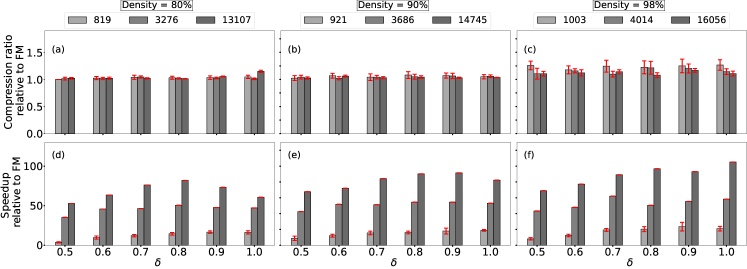
Figure 4: CPGC vs. FM: Compression ratio relative to FM (top row: (a), (b) and (c)) and speedup relative to FM (bottom row: (d), (e) and (f)) for graphs with 819 to 16 thousand edges.

Average running time. We observe that for the same $\delta$ and density, the running time increases as the number of vertices increases which is expected (CPGC running time is $O(mn^{\delta})$). We also observe that for the same $n$ and density, the running time decreases as $\delta$ increases. For instance, with $m=214.75$ million for density = 0.80 and $\delta=0.5$, the running time is 176.27 seconds, whereas for $\delta=1$ it reduces to 117.8 seconds. This is because of the relation between $\delta$ and $\hat{k}$ described earlier, CPGC cannot find a large set of common neighbours which results in a lower compression ratio for lower density. Also, when CPGC does not find an edge with $u_{i}\in U$ for any vertex $w_{j}\in K_{q}$, then it skips to the next vertex in $U$ to check for an edge with $w_{j}\in K_{q}$ thus, decreasing the running time. Therefore, we do not observe an increase in the running time as $\delta$ increases. However, for density = 0.98, the running time decreases as $\delta$ increases, even when the compression ratio increases. For example, with $m=1.05$ billion for density = 0.80 and $\delta=0.5$, the running time is 164.83 seconds, whereas for $\delta=1$ the running time is 150.97 seconds. This is because for higher density and large $\delta$, large $\delta$-cliques are extracted which decreases the total number of iterations performed by CPGC and subsequently reduces the running time.

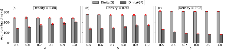
Figure 5: Dinitz($G$) vs. Dinitz($G^{*}$): Average running time of Dinitz’s algorithm on the original bipartite graph $G$ (labeled Dinitz($G$)) and on the compressed graph $G^{*}$ (labeled Dinitz($G^{*}$)), for a large graph with approximately 32,000 vertices in each bipartition and 214.75 million to 1.05 billion edges corresponding to densities = $0.80,0.90,$ and $0.98$ and different $\delta$.

5.2 Results for Small Graphs.

In this section, we compare the performance of CPGC against FM on small graphs, particularly, on graphs with $n=2^{i}$ vertices in each bipartition, where $i$ ranges from 5 to 7 and the number of edges ranging from 819 to 16,056. However, due to the limitations of FM as previously mentioned, our comparison is constrained to $n=2^{7}$ and $m=16,056$. We compare the performance of the two algorithms using two metrics, relative compression ratio, and relative speedup.

Compression ratio relative to FM. We define the compression ratio relative to FM, as the ratio of compression ratio achieved by CPGC and FM. Figures 4a-4c show the relative compression ratio relative to FM achieved by CPGC in the case of small graphs, for $\delta=0.5,0.6,0.7,0.8,0.9,1$, and densities = 0.80, 0.90, 0.98. In all cases, the relative compression ratio ranges from $1$ to $1.27$, highlighting that the compression ratio achieved by CPGC is at least as that of FM. CPGC achieves a greater compression ratio than FM because it extracts multiple $\delta$-cliques before $\hat{k}$ decreases as shown in Figure 2(b), resulting in removing more edges at higher values of $\hat{k}$ (Section 3.2). We observe that CPGC achieves a compression ratio equal to that of FM for a small graph with $n=32$, $m=819$, density = 0.80, and $\delta=0.5$. This is because a small graph does not require many iterations for extracting $\delta$-cliques, thereby not giving CPGC the opportunity to extract more cliques over the FM algorithm. However, for the same $n$ and $\delta$ when the graph density increases the compression ratio achieved by CPGC also increases. For example, with $n=32$, $m=921$, and $1,003$, the relative compression ratio is 1.03 and 1.25, respectively. As explained before, certain combinations of $n$, $m$, and $\delta$ lead to the highest compression ratio. For instance, when $n=128$, $m=16,056$ for a density of 0.98, we observe that the relative compression ratio initially increases from 1.1 to 1.14 with increasing $\delta$ from 0.5 to 0.7. However, further increasing $\delta$ to 1 results in a decrease in the relative compression ratio to 1.1.

Speedup relative to FM. We define the speedup relative to FM as the ratio of the runing time of FM over CPGC. Figures 4d-f illustrate the speedup achieved by CPGC for bipartite graphs with $n$ = 32, 64, and 128 vertices in each partition, $m$ = 819 to 16 thousand for densities of 0.80, 0.90, and 0.98, and $\delta$ values ranging from 0.5 to 1. The running time of CPGC is consistently lower than that of FM, resulting in speedup by CPGC across all cases. This is primarily due to the selection of vertices in the while loop (Lines 4-6) in CSA, facilitating faster compression by extracting more than one i.e., $\gamma$, $\delta$-cliques in a single iteration, as shown in Figure 2(b). The speedup increases notably with higher $\delta$ and density. For example, with $n=32$ and $m=819$ for density 0.8, CPGC achieves an average speedup of 3.66 for $\delta=0.5$, increasing to 16.28 for $\delta=1$. Similarly, with $n=32$ and $\delta=1$, CPGC achieves an average speedup ranging from 16.28 for $m=819$ with density 0.8 to 20.97 for $m=16$ thousand with density 0.98. It is worth noting that for small graphs, certain combinations of $n$, $m$, and $\delta$ yield higher speedup values. For instance, with $n=128$ and $m=819$ for density 0.8, the speedup increases from 52.81 to 81.97 for $\delta=0.8$, and then slightly decreases to 60.68 for $\delta=1$.

5.3 Speeding-up Matching Algorithms.

Since the compressed representation of the original graph maintains all the path information, it can be used as input to other graph algorithms such as maximum cardinality matching, to speedup their execution. Consider Dinitz’s algorithm [6] for finding the maximum cardinality matching in a bipartite graph, whose running time is in $O(\sqrt{n}m)$. According to Theorem 4.3 the compression ratio of CPGC is $k=\Omega\Big{(}\frac{\delta\log n}{\log(2n^{2}/{m})}\Big{)}$, where $0<\delta<1$. This is the same as the compression ratio achieved by FM [9]. Because the number of edges in the compressed graph is reduced by a factor of $k$, using CPGC as preprocessing for Dinitz’s algorithm leads to a total time of $O(\sqrt{n}m/k+mn^{\delta})$. For $\delta<1/2$, the total running time becomes $O(\sqrt{n}m\log_{n}{(\frac{n^{2}}{m}}))$. To the best of our knowledge, this matches the best known asymptotic bound for maximum cardinality bipartite matching algorithms (also achieved by employing FM instead of CPGC and by the bipartite matching algorithm based on push-relabel method [10]). Similar reasoning applies if instead of Dinitz’s algorithm we consider the Hopcroft-Karp algorithm [11].

Figure 5 shows the average running time of Dinitz’s algorithm on the original bipartite graph $G$ with $n=32$ thousand vertices in each bipartition, and $m$ ranging from 214.75 million to 1.05 billion edges for densities = $0.80,0.90,$ and $0.98$ and different $\delta$. It also shows the run time of Dinitz’s algorithm executed on the compressed tripartite graph $G^{*}$, for different values of $\delta$, and densities $=0.80,0.90,$ and $0.98$. We observe that in all cases the Dinitz algorithm applied to the compressed graph $G^{*}$ outperforms its execution on the original graph $G$, achieving a reduction in the running time of up to 72.83%. Even when considering the preprocessing time required to compress the graph $G$, the running time of the Dinitz algorithm for large, dense graphs is still reduced by up to 25.09% with the compressed graph $G^{*}$. This reduction in the running time is directly proportional to the level of compression achieved, where larger compression ratios result in reduced running time. For instance, as discussed in the context of large graphs (Figure 3(a-c)), for a density of $0.98$, CPGC demonstrates an increasing compression ratio as the edge count $m$ reaches 1.05 billion with increasing values of $\delta$. Consequently, the run time of Dinitz’s algorithm on the compressed graph $G^{*}$ also decreases.

6 Conclusion and Future Work

We proposed a new algorithm for graph compression based on partitioning the graph into bipartite cliques. The proposed algorithm runs in time $O(mn^{\delta})$ which improves over the $O(mn^{\delta}\log^{2}n)$ time of the Feder-Motwani (FM) algorithm (the best existing clique partitioning-based graph compression algorithm). Our algorithm achieves an average compression ratio at least as good as that of FM. Experimental results showed that our algorithm achieved a compression ratio of up to 26% greater than that obtained by FM and executes up to 105.18 times faster than FM. We also investigated the reduction in running time of a cardinality matching algorithm (Dinitz’s algorithm) when using the compressed graph instead of the original graph. The results showed that for sufficient large dense graphs, using the compressed graph obtained by CPGC as an input to the matching algorithm leads to a reduction in the running time of up to 72.83% over the matching algorithm using the original graph. In future work, we plan to continue investigating the graph compression problem and propose algorithms that improve over the compression ratio obtained by our proposed algorithm.

A Appendix

A.1 FM algorithm.

In Algorithm 3 we give a high-level description of the FM algorithm. The FM algorithm first constructs neighborhood trees for each vertex $u_{i}$ in $U$, which are labeled binary trees of depth $r$, whose nodes are labeled by a bit string $\omega$, where $0\leq|\omega|\leq r$. The root node of a neighborhood tree contains all the vertices in $W$ and is labeled by the empty string, $\epsilon$. The bit string $\omega$ of a node is obtained by starting at the root and following the path in the tree up to the node and concatenating a 0 or a 1 to $\omega$ each time the path visits the left, or the right child, respectively. The nodes at level $i$ in the tree correspond to a partition of $W$ into sets of size $|W|/2^{i}$. Thus, each leaf node corresponds to a vertex in $W$. Each node in the neighborhood tree of $u_{i}$ stores $d_{i,\omega}$, the number of neighbors of $u_{i}$ in the set $W_{\omega}$ of vertices of $W$ that are associated with the node with label $\omega$, i.e., $d_{i,\omega}=|N(u_{i})\cap W_{\omega}|$, where $N(u_{i})$ is the set of the neighbors of $u_{i}$. In Figure 1(b), we show the neighborhood tree of vertex $u_{2}$ for the bipartite graph with $|U|=|W|=n=8$ given in Figure 1(a). Vertex $w_{3}$ is a leaf and would have $\omega=010$ in all neighborhood trees of the graph.

Algorithm 3 FM Algorithm: High-level description

1:$G(U,W,E)$: Bipartite graph;

2:Initialize: clique index, $q\leftarrow 0$; no. of vertices $n\leftarrow|U|$; and no. of remaining edges $\hat{m}\leftarrow|E|$.

3:Build neighborhood trees for vertices $u_{i}\in U$.

4:while $\hat{m}\geq n^{2-\delta}$ do

5:  $\hat{k}\leftarrow\bigg{\lfloor}{\frac{\delta\log n}{\log(2n^{2}/\hat{m})}}\bigg{\rfloor}$

6:   Starting with $t=1$ and $U_{t}=U$, iterate while $t\leq\hat{k}$ to select $\hat{k}$ vertices based on $c_{0}$ and $c_{1}$ (calculated as in Equation A.1) to form the ordered set $K_{q}=\{y_{1},y_{2},\ldots,y_{t}\}\subseteq W$. At each stage $t$, obtain set $U_{t+1}=\left\{u\in U_{t}\mid y_{1},\ldots,y_{t}\in N(u)\right\}$ which omits vertices from $U$ that are not adjacent to $K_{q}$. And update the corresponding neighborhood trees such that $d_{i,\omega}$ of the nodes along the path from root to the selected vertex is decreased by 1 for each neighborhood tree corresponding to $U_{t}$.

7:   Form the $\delta$-clique $C_{q}=(U_{q},K_{q})$, where, $U_{q}=U_{t}$.

8:  Update $G$ by removing the edges associated with clique $C_{q}$ and update $\hat{m}\leftarrow|E|$.

9:  $q\leftarrow q+1$

10:For each clique in $\mathcal{C}=\{C_{1},\ldots,C_{q}\}$ add edges from all the vertices in the left partition $U_{q}$ to an additional vertex $z_{q}$, and from $z_{q}$ to all the vertices in the right partition $K_{q}$. This would compress the graph by replacing $|U_{q}|\times|K_{q}|$ edges with $|U_{q}|+|K_{q}|$ edges.

11:The remaining edges in $G$ are trivial cliques and are added in the compressed graph $G^{*}$.

12:Output: $G^{*}$, the compressed graph of $G$.

The algorithm computes $\hat{k}$ and then, in Line 5, it performs $\hat{k}$ iterations (indexed by $t$) to select vertices for the right partition of clique $C_{q}$. In each iteration it selects vertices at leaf nodes of the neighborhood trees by following a path based on $d_{i,\omega}$ of child nodes and the number of distinct ordered subsets of the neighbourhood tree at each level. In order to select a path at each level, the algorithm calculates $c_{0}$ and $c_{1}$ as follows:

(A.1) $$c_{j}=C\left(U_{t},\mathscr{C}_{t,\omega\cdot j}\right)=\sum_{i:{u_{i}\in U_{t}}}d_{i,\omega\cdot j}\cdot\left(d_{i}-1\right)^{[{k}-t]},\,j=0,1.$$

$c_{j}$ counts the number of ordered sets in $\mathscr{C}_{t,\omega}$ whose elements are adjacent to $u_{i}$, where $\mathscr{C}_{t,\omega}$ denotes the collection of all ordered sets $K$ of $W$ of size $k$ in iteration $t$, with $t\leq k$. In each iteration, a vertex in $W$ is added to the right partition of the clique. If $|N(u_{i})|=d_{i}$, then the number of distinct ordered subsets of $N(u_{i})$ of size $k$ is $d_{i}^{[k]}$, where $d_{i}^{[k]}=d_{i}(d_{i}-1)(d_{i}-2)\cdots(d_{i}-k+1)$. Based on $c_{j}$’s, the FM algorithm chooses either the left node (if $c_{0}\geq c_{1}$) or the right node (if $c_{0}<c_{1}$). When the algorithm reaches a leaf node, it selects the corresponding vertex in $W$, updates the set of common neighbors ($U_{t}$), and decreases $d_{i,\omega}$ of each node along the path to the selected vertex by 1, in neighborhood trees corresponding to $U_{t}$. Thus, it guarantees the selection of a new vertex in the following iterations. The algorithm continues this process until it extracts $\hat{k}$ unique vertices to form the set $K_{q}$, the right partition of the $q$-th $\delta$-clique $C_{q}$.

After forming set $K_{q}$, the FM algorithm proceeds to identify the common neighbors of the vertices that are part of set $K_{q}$ in order to construct $U_{q}$, which is the left partition of the $q$-th $\delta$-clique $C_{q}$. The pair $(K_{q},U_{q})$ forms a $\delta$-clique $C_{q}$. Subsequently, the algorithm updates $\hat{m}$, the number of remaining edges in the graph after extracting each $\delta$-clique. This update is done by subtracting the product of the sizes of $K_{q}$ and $U_{q}$ from $\hat{m}$, i.e., $|U_{q}|\times|K_{q}|$. The algorithm then updates $\hat{k}$ considering the updated value of $\hat{m}$ and repeats the procedure to extract more $\delta$-cliques until no more $\delta$-cliques can be found (determined by the condition of the while loop). The edges that are not removed in this process form trivial cliques.

The FM algorithm compresses the graph by adding a new vertex set $Z$ to the bipartite graph, thus converting it into a tripartite graph (Figure 1(c)), where each vertex in $Z$ corresponds to one clique extracted by the algorithm. Each vertex of the left and right partitions of $\delta$-clique $C_{q}$ is then connected via an edge to a new vertex $z_{q}\in Z$, thus forming a tripartite graph. This decreases the number of edges from $|U_{q}|\times|K_{q}|$ to $|U_{q}|+|K_{q}|$, thus compressing the graph. The compressed graph obtained by the algorithm preserves the path information of the original graph. The running time of the FM algorithm is $O(mn^{\delta}\log^{2}n)$. The FM algorithm can be extended to the case of non-bipartite graphs, where it computes a compression of a graph in time $O(mn^{\delta}\log^{2}n)$, as shown by Feder and Motwani [9].

A.2 Example: CPGC Execution.

We now show how CPGC works on a bipartite graph $G$ with partitions $U$ and $W$, $n=|U|=|W|=8$, and $|E|=54$, shown in Figure 6(a). CPGC (Algorithm 1), first initializes $q=0,n=|W|=|U|=8,\hat{m}=|E|=54,\mathcal{C}=\emptyset$, and $d_{w}=[0]_{n}$. It then calculates the degree of each vertex $d_{w_{j}}$ in Lines 2-4, as shown in Table 1. It calculates $\hat{k}(n,m,\delta)=2$ in Line 5. Thus, the condition for the while loop in Line 6 is met and CPGC calls CSA in Line 7. With the given inputs, CSA sorts $d_{w}$ in non-increasing order. Let $\{w_{4},w_{2},w_{3},w_{5},w_{6},w_{1},w_{7},w_{8}\}$ be the non-increasing order with corresponding degrees given as $d_{w_{\pi(j)}}$ in Table 1.

CPGC step	$j$	1	2	3	4	5	6	7	8
Initialization	$d_{w_{j}}$	6	7	7	8	7	7	6	6
Sorted $d_{w_{j}}$	$d_{w_{\pi(j)}}$	8	7	7	7	7	6	6	6
After $1^{st}$iteration	$d_{w_{j}}$	6	0	0	1	0	7	6	6

Table 1: Degrees of vertices in partition $W$ at different steps of CPGC.

(a)

(b)

(c)

(d)

(e)

Figure 6: Clique partitioning: (a) given bipartite graph $G(U,W)$; (b) extracted clique $C_{1}$; (c) extracted clique $C_{2}$; (d) graph with trivial cliques; and (e) compressed tripartite graph $G(U,Z,W)$

In Line 5, CSA forms set $\mathcal{K}$, where $\mathcal{K}=\{w_{4},w_{2},w_{3},w_{5},w_{6}\}$ has all vertices whose degrees are greater than or equal to $d_{w_{\pi(\hat{k})}}=7$. This results in $\gamma=2$ in Line 7, therefore CSA extracts two cliques in Lines 8-13. Since $q$ is initialized to 0 in CPGC, the for loop in Line 8 iterates two times for $c=1$ and $2$. In Line 9, CSA forms $K_{1}=\{w_{4},w_{2}\}$, and in Line 10, it forms the left partition $U_{K_{1}}$ of bipartite clique $\mathcal{C}_{1}$, by selecting the common neighbors of the vertices in $K_{1}$. For example, for set $K_{1}=\{w_{4},w_{2}\}$, $U_{K_{1}}=U-\{u_{7}\}$ as $w_{4}$ and $w_{2}$ have $\{u_{1},u_{2},u_{3},u_{4},u_{5},u_{6},u_{8}\}$ as common neighbors. In Line 12, CSA updates the adjacency matrix $A$ by removing the edges of bipartite clique $\mathcal{C}_{1}$ from the original bipartite graph $G$ and finally in Line 13, it updates all $d_{w}$ by subtracting $|U_{K_{1}}|=7$ from both $d_{w_{4}}$ and $d_{w_{2}}$, thus $d_{w_{4}}=1$ and $d_{w_{2}}=0$. Similarly, when $c=2$, $K_{2}=\{w_{3},w_{5}\}$ and $U_{K_{2}}=U-\{u_{6}\}$. CSA updates the adjacency matrix $A$ and $d_{w}$ such that $d_{w_{3}}=d_{w_{5}}=0$. Therefore, in the first execution, CSA, forms two bipartite cliques and removes a total of $(7\times 2)+(7\times 2)=28$ edges from $G$. The updated degrees of the vertices are shown in Table 1. It then forms the set of bipartite cliques extracted in the current execution in Line 14, $\mathscr{C}=\{C_{1},C_{2}\}$. The two cliques are shown in Figures 6(b) and 6(c).

CSA returns $(\mathscr{C},\hat{A},\hat{d}_{w})$ and then CPGC updates the set $\mathscr{C}=\{C_{1},C_{2}\}$, $d_{w}$, the adjacency matrix $A$, and the number of edges $\hat{m}=54-28=26$, in Lines 8-10. In Line 12, CPGC updates $q=2$ and finally, in Line 13 it updates $\hat{k}$ according to the new value of $\hat{m}$ in Line 11 which results in $\hat{k}=1$. Since $\hat{k}=1$, it means CPGC extracts only trivial bipartite cliques (shown in Figure 6(d)) which do not contribute to graph compression. Thus, it does not meet the condition in the while loop (Line 6) and CPGC terminates.

CPGC then compresses the graph by adding two vertices, $z_{1}$, and $z_{2}$, corresponding to the two cliques $C_{1}$ and $C_{2}$, and adds the corresponding edges to form the tripartite graph. The edges in the given graph $G(U,W,E)$, that are not part of any $\delta$-clique are connected directly as shown in Figure 6(e).

A.3 Proofs

Proof of Theorem 4.1.

• Let’s assume that CPGC extracts only one $\delta$-clique $C_{q}$ from the given graph $G$. In the $\delta$-clique $C_{q}$, the right partition $K_{q}\subseteq W$ is formed by selecting $\hat{k}$ vertices from $W$ and the left partition $U_{q}\subseteq U$ is formed with the common neighbors of $K_{q}$, forming a complete bipartite graph with $E_{q}$ edges. The compressed graph $G^{*}$ is formed with the same left and right partitions $U$ and $W$ of the graph $G$, and a third partition $Z$ which is a set of additional vertices associated with each of the $\delta$-cliques that CPGC extracts. Our main concern is with the edges $(u_{i},w_{j})\in E^{*}$ in the compressed graph $G^{*}$. $E^{*}$ contains the edges that replace the $\delta$-clique $C_{q}$ by adding the additional vertex $z_{q}\in Z$, and the set of edges $\hat{E}=E\setminus E_{q}$ which were not part of the $\delta$-clique $C_{q}$. It can be easily seen that $\hat{E}\subset E$, that is, the edges in $\hat{E}$ are edges in $G$, and the remaining edges $E^{*}\setminus\hat{E}$ in $E^{*}$ are the edges that replace $C_{q}$ in $G^{*}$. Each edge $(u_{i},w_{j})\in E_{q}$, is replaced by two edges, $(u_{i},z_{q})$ and $(z_{q},w_{j})$, where $u_{i}\in U$, $w_{j}\in W$, and $z_{q}\in Z$. Therefore, for each edge $(u_{i},w_{j})\in E_{q}$, there exists a path from $u_{i}$ to $w_{j}$ composed of two edges, $(u_{i},z_{q})$ and $(z_{q},w_{j})$, that passes through the additional vertex $z_{q}\in Z$, thus preserving the path information. This holds true for all the $\delta$-cliques extracted by CPGC.          

Proof of Lemma 4.1.

• In the $\delta$-clique based graph compression performed by CPGC, the compressed graph $G^{*}(U,W,Z,E^{*})$ is obtained from $G$ by replacing $|E_{q}|=|U_{q}\times K_{q}|$ edges in a $\delta$-clique $C_{q}$ with $|E^{*}|=|U_{q}|+|K_{q}|$ edges in $G^{*}$ and adding an additional vertex $z_{q}\in Z$ for each extracted $\delta$-clique $C_{q}$. The size of the right partition of $C_{q}$ is $|K_{q}|={k}=k(n,m,\delta)=\Big{\lfloor}{\frac{\delta\log n}{\log(2n^{2}/m)}}\Big{\rfloor}$. If $m<2n^{2-\frac{\delta}{2}}$ then the size of the right partition $|K_{q}|$ is $k=1$. Therefore, the number of edges in the $\delta$-clique is $|E_{q}|=|U_{q}|\cdot 1=|U_{q}|$. Those edges are replaced by $|E^{*}|=|U_{q}|+\hat{k}=|U_{q}|+1$ edges in $G^{*}$. Thus, replacing the $\delta$-clique in $G$ with $m<2n^{2-\frac{\delta}{2}}$, the number of edges in $G^{*}$ would actually increase by 1, which does not lead to a compression of $G$.          

A.4 Extension to non-bipartite graphs.

CPGC can be extended to compress non-bipartite graphs using a similar technique to that described in [9]. Consider a directed graph $H(V,E)$ with $n$ vertices and $m$ edges. Initially, we transform $H$ into a bipartite graph $G\left(L,R,E^{\prime}\right)$, where each vertex $v\in V$ is duplicated into $v_{L}\in L$ and $v_{R}\in R$. For each directed edge $(u,v)$ in $E$, we create a directed edge $\left(u_{L},v_{R}\right)$ in $E^{\prime}$, with the direction from $L$ to $R$. Furthermore, for each vertex $v\in V$ we add a directed edge from $v_{R}$ to $v_{L}$. The proposed compression algorithm is then applied to the bipartite graph $G$, which includes only the edges from $L$ to $R$. Once the compressed graph is computed we add to it the $n$ directed edges from $u_{R}$ to $u_{L}$, corresponding to each vertex $u\in V$. Since the path information of the original graph is preserved by this transformation, it allows different graph algorithms to work on the compressed graph as well. Undirected general graphs can be transformed first into directed graphs by simply replacing each undirected edge $(u,v)$ in the original graph by two directed edges $(u,v)$ and $(v,u)$, and then applying the technique presented above to transform the directed graph into a bipartite graph. The time complexity and the compression ratio of CPGC are the same as in the case of the bipartite graphs. A similar approach for converting a general graph to a bipartite graph and then compressing the obtained bipartite graph was employed in [3, 5].

References

- [1] Max Bannach, Florian Andreas Marwitz, and Till Tantau. Faster Graph Algorithms Through DAG Compression. In Olaf Beyersdorff, Mamadou Moustapha Kanté, Orna Kupferman, and Daniel Lokshtanov, editors, 41st International Symposium on Theoretical Aspects of Computer Science (STACS 2024), volume 289 of Leibniz International Proceedings in Informatics (LIPIcs), pages 8:1–8:18, Dagstuhl, Germany, 2024. Schloss Dagstuhl – Leibniz-Zentrum für Informatik.
- [2] Maciej Besta and Torsten Hoefler. Survey and taxonomy of lossless graph compression and space-efficient graph representations. CoRR, abs/1806.01799, 2018.
- [3] Gregory Buehrer and Kumar Chellapilla. A scalable pattern mining approach to web graph compression with communities. In Proceedings of the 2008 International Conference on Web Search and Data Mining, WSDM ’08, page 95–106, New York, NY, USA, 2008. ACM.
- [4] Maximilien Danisch, Ioannis Panagiotas, and Lionel Tabourier. Compressing bipartite graphs with a dual reordering scheme. CoRR, abs/2209.12062, 2022.
- [5] Laxman Dhulipala, Igor Kabiljo, Brian Karrer, Giuseppe Ottaviano, Sergey Pupyrev, and Alon Shalita. Compressing graphs and indexes with recursive graph bisection. In Proceedings of the 22nd ACM SIGKDD International Conference on Knowledge Discovery and Data Mining, KDD ’16, page 1535–1544, New York, NY, USA, 2016. ACM.
- [6] Yefim Dinitz. Algorithm for solution of a problem of maximum flow in a network with power estimation. Doklady Akademii Nauk SSSR, 11:1277–1280, 1970.
- [7] Shimon Even and R. Endre Tarjan. Network flow and testing graph connectivity. SIAM Journal on Computing, 4(4):507–518, 1975.
- [8] Wenfei Fan, Yuanhao Li, Muyang Liu, and Can Lu. Making graphs compact by lossless contraction. In Proceedings of the 2021 International Conference on Management of Data, SIGMOD ’21, page 472–484, New York, NY, USA, 2021. ACM.
- [9] T. Feder and R. Motwani. Clique partitions, graph compression and speeding-up algorithms. Journal of Computer and System Sciences, 51(2):261–272, 1995.
- [10] Andrew V. Goldberg and Robert Kennedy. Global price updates help. SIAM J. Discret. Math., 10(4):551–572, August 1997.
- [11] John E. Hopcroft and Richard M. Karp. An algorithm for maximum matchings in bipartite graphs. SIAM Journal on Computing, 2(4):225–231, 1973.
- [12] David W. Matula. Determining edge connectivity in 0(nm). In Proc. of the 28th Annual Symposium on Foundations of Computer Science, SFCS ’87, page 249–251, 1987.
- [13] Ryan Rossi and Rong Zhou. Graphzip: a clique-based sparse graph compression method. Journal of Big Data, 5, 03 2018.