Distribution Transformers: Fast Approximate Bayesian Inference With On-The-Fly Prior Adaptation

Abstract

While Bayesian inference provides a principled framework for reasoning under uncertainty, its widespread adoption is limited by the intractability of exact posterior computation, necessitating the use of approximate inference. However, existing methods are often computationally expensive, or demand costly retraining when priors change, limiting their utility, particularly in sequential inference problems such as real-time sensor fusion. To address these challenges, we introduce the Distribution Transformer—a novel architecture that can learn arbitrary distribution-to-distribution mappings. Our method can be trained to map a prior to the corresponding posterior, conditioned on some dataset—thus performing approximate Bayesian inference. Our novel architecture represents a prior distribution as a (universally-approximating) Gaussian Mixture Model (GMM), and transforms it into a GMM representation of the posterior. The components of the GMM attend to each other via self-attention, and to the datapoints via cross-attention. We demonstrate that Distribution Transformers both maintain flexibility to vary the prior, and significantly reduces computation times—from minutes to milliseconds—while achieving log-likelihood performance on par with or superior to existing approximate inference methods across tasks such as sequential inference, quantum system parameter inference, and Gaussian Process predictive posterior inference with hyperpriors.

1 Introduction

Modern machine learning has transformed many data-rich domains (LeCun et al., 2015), yet critical applications like healthcare diagnostics and autonomous vehicle safety demand more than just predictive accuracy (Hüllermeier & Waegeman, 2019). These high-stakes settings, often characterized by limited or noisy data, require robust uncertainty estimation and principled integration of domain knowledge (Gawlikowski et al., 2021)—capabilities naturally addressed through probabilistic reasoning.

Bayesian inference is a cornerstone of probabilistic machine learning, encoding prior beliefs and providing the tools to incorporate new observations while providing principled uncertainty quantification; essential for critical decision-making under uncertainty. However, Bayesian inference is typically intractable, limiting its real-world adoption. To counteract this problem, the field of approximate inference has emerged, providing a range of methods: Variational inference (VI) methods (Blei et al., 2016) can approximate posterior densities but require expensive optimization procedures at inference time (as opposed to training time, relevant for later methods). While Markov Chain Monte Carlo (MCMC) (Christian & Casella, 2011) methods provide asymptotically-exact posterior samples, they neither directly estimate the density nor offer the rapid inference often required in practical applications.

Recent advances in deep learning have opened new avenues for Bayesian inference. Prior Fitted Networks (PFNs) (Muller et al., 2021) demonstrated that transformer (Vaswani et al., 2017) architectures can perform Bayesian inference through a single forward pass, dramatically reducing inference time compared to traditional methods. However, PFNs are limited by their dependence on a fixed prior, requiring costly retraining for each new prior distribution encountered. In practice, it is often desirable, and in some applications essential, to be able to change the prior rapidly at inference time.

While these methods have their strengths, there remains a clear need for approximate inference methods that can provide accurate posterior density estimates with minimal computational overhead while maintaining the flexibility to modify priors at inference time. To address this need, we introduce Distribution Transformers (DTs), a novel transformer-based architecture that combines the flexibility of VI with the efficiency of PFNs. Our method generates posterior density estimates through a single forward pass while handling a range of prior distributions from a given parametric family without retraining. Unlike traditional VI approaches that often rely on simple parametric families, DTs leverage a expressive distributional family that can universally approximate smooth densities. Figure 2 illustrates the architectural design of DTs. Fundamentally, DTs approximate the prior with a Gaussian Mixture Model (GMM) represented as an embedded sequence in the latent space of the transformer, then condition this GMM on observations using a permutation-equivariant transformer decoder, yielding a GMM approximation to the posterior.

DTs are trained using entirely sample-based supervised learning by defining a joint distribution over the prior, parametrized by $\phi$, the latent variable $x$, and the observations $z$. We demonstrate that this training approach yields an approximator of exact posterior prediction. This combination of speed, flexibility, and expressiveness enables accurate Bayesian inference in scenarios where existing methods face fundamental limitations. Concretely, DTs address the key challenges discussed above, providing accurate posterior density estimates for a wide range of priors. Like PFNs, our approach only requires a way to sample from the chosen prior family and an arbitrary likelihood model, and is widely applicable without significant task-specific analysis. We make the following contributions:

1. We introduce Distribution Transformers (DTs)—a novel architecture that leverages the power of universally-approximating Gaussian Mixture Models and Transformers to express arbitrary distribution-to-distribution mappings.

2. We show that DTs can be trained to perform more accurate approximate Bayesian inference, and up to orders of magnitude faster, than existing approximate inference methods, while also allowing on-the-fly updates to the prior at inference time without retraining, a never before accomplished feat.

3. We empirically demonstrate near-exact inference capabilities on challenging problems, including joint PPD-hyperposterior approximations for Gaussian Processes (GPs), parameter inference for quantum systems and a real-world sequential inference task, while remaining fast enough for real-time applications.

1.1 Related Work

Bayesian inference aims to determine the posterior distribution $p(x\mathop{|}z)$ of a latent variable $x$ given observations $z$, using Bayes’ theorem: $p(x\mathop{|}z)=\frac{p(z\mathop{|}x)p(x)}{p(z)}$. While closed-form posteriors exist for specific conjugate prior scenarios, the general case involves an intractable evidence integral $p(z)=\int p(z\mathop{|}x)p(x)dx$ (along with others such as statistics of the predictive posterior distribution (PPD), for example), necessitating approximate inference methods.

Variational inference (VI) aims to approximate the posterior density through fitting a density of a particular family (typically a Gaussian) to the posterior by maximizing a variational lower bound on the evidence. Notable modern extensions include stochastic variational inference (SVI) (Hoffman et al., 2013), which utilizes backpropagation to optimize a stochastic approximation of the variational objective, black-box variational inference (Ranganath et al., 2014), which provides widely-applicable, model-agnostic tools for optimization of this variational objective, and amortized variational inference (AVI) (Kingma & Welling, 2014; Ganguly et al., 2023), which efficiently solves many variational inference problems in parallel through the learning of an inference network mapping from observations to approximate posteriors. These methods often provide acceptable estimates for the posterior density, but necessarily involve an expensive optimization routine at inference time, are not asymptotically exact, and often underestimate the posterior variance. Nonetheless, VI remains the most popular approximate inference technique in use today, and we will use a variant as a baseline in our empirical studies.

Recent neural approaches to approximate inference leverage the expressivity of deep learning architectures while aiming to maintain theoretical guarantees. Prior Fitted Networks (PFNs) (Muller et al., 2021) learn to perform approximate inference through sample-based supervised learning without the need for posterior densities (which are instead accessed via samples from the joint distribution over $x$ and $z$), enabling inference in a single forward pass. They provide rapid inference for changes in dataset, provide a posterior density estimate, and allow for almost arbitrary priors, but require complete retraining upon changes to the prior distribution, and use a Riemann Distribution, which can struggle to model smooth, heavy-tailed posteriors. As a close competitor to our method, we will also adopt a PFN baseline for our posterior studies.

Continuous normalizing flows (Rezende & Mohamed, 2015) learn a mapping from samples of some simple distribution to samples of the target posterior density, leveraging automatic differentiation to provide a flexible, closed-form density using a change of measure. However, the mapping they learn is fixed, meaning the prior is set at training time, and observations can only be incorporated via sufficient statistics of the simple distribution, limiting their suitability for our problem setting. Moreover, they must be constructed using only fully reversible components, which can limit expressivity. Classical approaches include the Laplace approximation (Tierney & Kadane, 1986) and expectation propagation (EP) (Minka, 2001). The Laplace approximation fits a Gaussian distribution based on the local geometry at the posterior mode, but lacks invariance to reparametrization. EP iteratively refines an isotropic Gaussian approximation to the posterior, but struggles with numerical stability.

Sampling-based methods, most notably Markov chain Monte Carlo (MCMC) methods, provide samples from the posterior which can be used to compute stochastic estimates for expectations with respect to said posterior. These are primarily based on access to the unnormalized posterior via the numerator of Bayes’ theorem. When a differentiable prior and likelihood model are available, the state-of-the-art No U-Turn Sampler (NUTS) (Hoffman & Gelman, 2011) can be used. NUTS is based on Hamiltonian Monte Carlo (HMC) (Brooks et al., 2012), which provides more efficient generation of posterior samples without problem-specific tuning of the algorithm. MCMC methods are asymptotically exact and almost universally applicable, but are typically expensive due to random walk behavior. They also do not provide direct access to a posterior density, and empirical density estimates can be sample inefficient.

Bayesian quadrature-based methods (Osborne et al., 2012) assign a probabilistic model, typically a GP, to the integrand of the evidence $p(z)$ (and in some cases the predictive posterior distribution PPD $p(y|x,z)=\int p(y|x)p(x\mathop{|}z)$), and use probabilistic numerical integration to estimate the evidence and PPD directly. These methods provide accurate uncertainty measures, and can handle noisy, black-box likelihood models, but are typically computationally expensive and scale poorly to high-dimensional problems, although recent advances in sparse-GPs (Binois & Wycoff, 2021) provide promising avenues to alleviate these scaling issues.

1.1.1 Sequential Inference

Sequential inference over time series requires dedicated methods, referred to as Bayesian filtering (when causality is required) or smoothing (when not). The extended Kalman filter (EKF) linearizes dynamics and observation models, then approximates the distribution over the latent state as a closed-form Gaussian. With modern automatic differentiation, this method is widely applicable and computationally efficient, but struggles in practice due to the overly restrictive assumptions induced by linearization and Gaussian distributions. Particle filters (PFs), or sequential Monte Carlo methods (Wills & Schön, 2023), maintain a population of particles which are distributed according to the posterior distribution each time step, but can be expensive and only provide an empirical density. The unscented Kalman filter (Julier & Uhlmann, 1997) maintains a minimal population of particles so is computationally efficient, but faces issues of numerical stability and also encodes a Gaussian assumption thus cannot handle multimodality. We compare our method against an EKF and a PF baseline.

2 Preliminaries

2.1 Transformers

The transformer architecture (Vaswani et al., 2017) has revolutionized deep learning, achieving state-of-the-art performance across domains including language modelling (Brown et al., 2020), computer vision (Dosovitskiy et al., 2020), and Bayesian inference (Muller et al., 2021). At its core, transformers learn mappings between sequences of tokens through the attention mechanism (Bahdanau et al., 2014), which enables parallelized information flow between sequence elements. This mechanism, combined with token-wise MLP layers, creates a parameter-efficient architecture capable of processing sequence elements in parallel.

Two theoretical properties of transformers are central to our work. First, transformers are universal sequence-to-sequence approximators (Yun et al., 2019), capable of representing arbitrary mappings between sequences. Second, in the absence of positional encodings, transformers are permutation equivariant with respect to the input sequence—a property we will exploit in Section 3.

Our method specifically employs the transformer decoder architecture. This architecture extends the base transformer by incorporating global cross-attention layers, allowing each position in the input sequence to attend to a separate context sequence. This cross-attention mechanism provides a natural framework for conditioning sequence transformations on observed data.

2.2 Gaussian Mixture Models

Gaussian Mixture Models (GMMs) are flexible probability distributions whose density is a weighted sum of Gaussian components, i.e. $q(x)=\sum_{i}w_{i}\mathcal{N}(x;\mu_{i},\Sigma_{i})$ where $\mathcal{N}(x;\mu,\Sigma)$ is a Gaussian density over $x,w_{i}\in[0,1]$, $\sum_{i}w_{i}=1$, $\boldsymbol{\mu}_{i}\in\mathbb{R}^{n}$, and $\boldsymbol{\Sigma}_{i}\in\mathbb{S}_{++}^{n}$, illustrated in Figure 1. While GMMs are widely used in clustering (Dempster et al., 1977), and latent variable modelling (Bishop, 2006), we focus on their role as universal approximators of smooth probability distributions (Goodfellow et al., 2016; Calcaterra & Boldt, 2008)—a property we exploit in Section 3. This universality extends to distributions on compact domains under appropriate change of measure, also illustrated in Figure 1. While the idea of using GMMs for function approximation is not new to deep learning (for example Bishop (1994) proposes the use of a GMM to model uncertainty in the output of a neural network), the idea of operating end-to-end on a distribution represented as a GMM is novel.

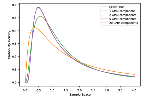
Figure 1: Various log-warped GMM approximation to an inverse-gamma prior distributions. Note that even with only five GMM components, the approximation is visually almost indistinguishable from the target distribution. This is true for many frequently encountered distributions in Bayesian inference.

A key property of GMMs is their natural representation as an unordered sequence of component parameters. Specifically, a $k$-component GMM over $\mathbb{R}^{n}$ is parametrized by $\boldsymbol{\theta}=\{(w_{i},\boldsymbol{\mu}_{i},\boldsymbol{\Sigma}_{i})\}_{i=1}^{k}$. This representation is permutation invariant—the ordering of components does not affect the resulting distribution.

Fitting a GMM to a given probability distribution is non-trivial, with methods such as expectation maximization and variational methods suffering from similar problems to their approximate inference counterparts. We will show that DTs naturally provide a mapping from the parameters of a given distribution to an approximating GMM without introduction of additional model parameters.

2.3 Amortization

Amortized methods have received significant attention from the machine learning, statistics, and optimization communities, owing to their ability to address computational bottlenecks in repetitive tasks. These methods learn to solve a class of optimization or simulation problems by incurring a substantial up-front computational cost during training, assuming the existence of some common structure between the solutions to these problems. This initial investment is offset by enabling the rapid solution of many subsequent problems, significantly reducing the overall computational burden over the model’s lifetime.

Amortized variational inference (AVI) (Ganguly et al., 2023; Kingma & Welling, 2014) exemplifies this paradigm, where a neural network is trained to approximate posterior distributions across multiple datasets, bypassing the need for iterative optimization for each new dataset. Similarly, PFNs (Muller et al., 2021) implicitly amortize inference through the learning of a mapping from observations to approximate posterior distributions without iterative updates. These examples highlight how amortization enables scalability and efficiency in otherwise computationally intensive workflows. As we shall show in Section 3, our work is also well-set in the context of amortized methods.

3 Distribution Transformers

Given a prior distribution $p(x\mathop{|}\phi)$ from a parametric family with parameters $\phi\in\Phi$ and observations $z\in\mathcal{Z}$ governed by likelihood $p(z\mathop{|}x)$, Bayesian inference aims to compute the posterior $p(x\mathop{|}z,\phi)$. Amortized approximate Bayesian inference reframes this as learning a mapping $\Phi\times\mathcal{Z}\to\mathcal{Q}$, where $\mathcal{Q}$ is a space of approximate posteriors. We introduce the Distribution Transformer (DT), a transformer-based architecture that directly maps priors and observations to posteriors. A core challenge in Bayesian inference is representing arbitrary probability distributions in a form suitable for neural networks. Our first key innovation is to represent all distributions as Gaussian Mixture Models (GMMs), which approximate any continuous density arbitrarily well. Our second key innovation is a transformer architecture that processes these mixtures as unordered sequences, preserving probabilistic structure while enabling expressive, scalable inference.

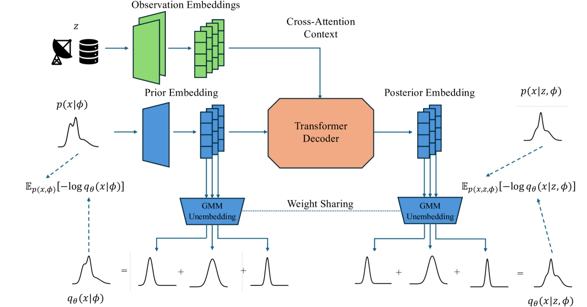
Figure 2: Architecture diagram for a distribution transformer. Observations, e.g. from a dataset or a sensor measurement, are transformed to a set of tokens in the latent space via a distinct learnable embedding for each datasource. Priors are represented as a set of embedded GMM components in the latent space via a learnable embedding acting on their parameters. The distribution transformer itself, a transformer decoder, learns to map the prior to the posterior in the latent space, incorporating information from the embedded observations via cross attention. A learnable unembedding acts token-wise on both the prior and posterior latent GMM representations to give a GMM approximation for both the prior and posterior distributions, with which we estimate our loss function $\ell_{\theta}^{\prime}.$

Figure 2 illustrates the DT architecture in detail. Conceptually, the DT architecture can be broken into four parts: the prior embedding, observation embeddings, transformer decoder and GMM unembedding.

Obtaining a GMM representation of an arbitrary prior is nontrivial. Inspired by Bishop (1994), we introduce a learnable embedding network that maps a prior’s parameters to a length-$k$ unordered sequence in the transformer’s latent space, representing an embedding of a $k$-component GMM approximation to the prior.

Observations $z$ vary widely (e.g., sensor readings, datasets). We use learnable embeddings tailored to different data sources, and embed datasets as sequences of data-label pairs embedded token-wise by a single embedding model. If a predictive posterior is needed, the query point is embedded separately. Observations are combined a unified latent sequence.

The transformer decoder maps the latent GMM prior representation to a posterior representation, conditioned on the observations via global cross-attention. We omit positional encodings to preserve permutation equivariance, aligning with the permutation invariance of the GMM sequence representation.

A GMM posterior approximation is then obtained via a learnable unembedding that acts component-wise on the posterior latent GMM unordered sequence, producing logits and normal densities. A cross-sequence softmax converts logits into component weights, and the approximating GMM can be constructed through summation of these components, achieving end-to-end permutation invariance of the architecture, as required.

Now that we have an architecture capable of mapping between distributions, we propose a sample-based training scheme with which to train our architecture to perform Bayesian inference. We must first introduce the concept of meta-priors $p(\phi)$—priors over priors representing the expected distribution of priors encountered by the algorithm. The only constraint on these meta-priors is that they can be sampled from, and can otherwise be quite complicated. For instance, in vehicle tracking, a meta-prior could constrain Gaussian means to a city’s road network while shaping covariance to reflect realistic uncertainties. Using this meta-prior, we can specify the joint distribution $p(\phi,x,z)$ hierarchically as $p(\phi)p(x\mathop{|}\phi)p(z\mathop{|}x)$. We may also specify a mapping $f(\cdot)$ from the sample space of interest to the sample space of the approximating GMM $\mathbb{R}^{n}$, for example to account for priors with finite support, essentially specifying a change of measure ensuring the probabilistic properties of the approximation are maintained. In this case, we denote the GMM itself as $q_{\theta}(f(x)\mathop{|}z,\phi)$, inducing the warped GMM $q_{\theta}(x\mathop{|}z,\phi)\approx p(x\mathop{|}z,\phi)$ under change of measure.

Algorithm 1 Training a Distribution Transformer

 Input: A joint distribution $p(\phi,x,z)$ over priors, latent variables and observations, the number of training iterations $m$, the batch size $b$, the number of GMM components $k$, and a mapping $f$ from the sample space of interest to the sample space of the GMM.

 Output: A mapping from $\phi$ and $z$ to warped GMMs $q_{\theta}(x\mathop{|}\phi)$ and $q_{\theta}(x\mathop{|}z,\phi)$ approximating the prior $p(x\mathop{|}\phi)$ and posterior $p(x\mathop{|}z,\phi)$ respectively.

 for $i=1$ to $m$ do

  Sample $\phi_{i}$, $x_{i}$ and $z_{i}$ from $p(\phi,x,z)$ for $i=1:b$;

  Estimate loss $\hat{\ell}^{\prime}_{\theta}=-\sum_{i=1}^{b}\log q_{\theta}(f(x_{i})\mathop{|}\phi_{i})+\log q_{\theta}(f(x_{i})\mathop{|}z_{i},\phi_{i})$;

  Update DT parameters with gradient descent on $\nabla_{\theta}\hat{\ell}^{\prime}_{\theta}$;

 end for

Outlined in Algorithm 1, DTs are trained to minimize $\ell_{\theta}^{\prime}$. Using meta-priors and a sample-space transform $f$, we extend the loss function proposed by Muller et al. (2021) another meta-level, defined as $\ell_{\theta}=\mathbb{E}_{p(\phi,x,z)}\left[-\log q_{\theta}(f(x)\mathop{|}z,\phi)\right]$. We show that this is equivalent to direct minimization of the KL-Divergence between the true posterior $p(x\mathop{|}z,\phi)$ and the GMM approximation $q_{\theta}(x\mathop{|}z,\phi)$:

Proposition 3.1.

The proposed loss $l_{\theta}$ equals the expected KL-Divergence $\mathbb{E}_{p(\phi,z)}\left[\text{KL}\left[p(\cdot\mathop{|}z,\phi)\mathop{||}q_{\theta}(\cdot\mathop{|}z,\phi)\right]\right]$ between $p(\cdot\mathop{|}z,\phi)$ and $q_{\theta}(\cdot\mathop{|}z,\phi)$ up to an additive constant. Proof in Appendix A.

The loss $l_{\theta}$ can be calculated stochastically using samples from the joint distribution $p(\phi,x,z)$, alleviating any need to directly access or sample from the posterior density.

Finally, DTs can jointly approximate priors and posteriors without additional model parameters. Applying the unembedding to the prior sequence yields a GMM approximation $q_{\theta}(x\mathop{|}\phi)$, extending DTs to mappings $\Phi\times\mathcal{Z}\rightarrow\Theta\times\Theta$. To ensure consistency, we introduce a prior loss:

$$\ell_{\theta}^{\text{prior}}=\mathbb{E}_{p(\phi,x)}\left[-\log q_{\theta}(x\mathop{|}\phi)\right],$$

leading to the combined objective: $\ell_{\theta}^{\prime}=\ell_{\theta}^{\text{prior}}+\ell_{\theta}$ .

4 Empirical Studies

We study the behaviour of our method in three settings: approximation of a tractable posterior, approximation of intractable posteriors, and a real-world sensor fusion problem posed as sequential inference. In the prior two settings, we benchmark our method against SVI (Hoffman et al., 2013), implemented in PyTorch (Paszke et al., 2019) with GPU parallelization, and PFNs (Muller et al., 2021), also implemented in PyTorch, fitting a Riemann distribution with the same number of model outputs as our DT. In the absence of a fixed prior, we train PFNs using the same sampling scheme as our method, effectively marginalizing out the meta-prior, leaving a less informative prior. We expect PFNs to perform well when the meta-prior is narrow and poorly when wide. For the latter experiment, we benchmark against the industry standard extended Kalman filter (EKF), and a particle filter (PF), again with GPU implementation. For the PF, we obtain a density via Gaussian kernel density estimation.

4.1 Analytical Verification Study

In specific cases, where the adopted prior is of a conjugate family to the likelihood, the posterior is tractable. We first verify that our approach does indeed perform approximate inference, for the case of an inverse-gamma prior and normal-variance likelihood. We choose a meta-prior consisting of independent inverse-gamma distributions over the rate and shape parameters, and test our approach on both narrow and wide parameter settings.

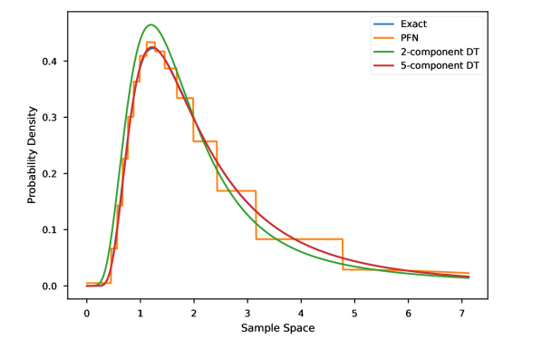
(a)

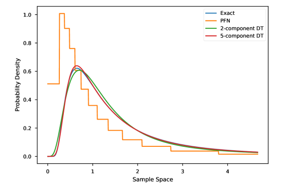
(b)

Figure 3: Ground truth, PFN, and 2 and 5 component DT posterior densities for an inverse-gamma prior with an (a) narrow and (b) wide meta-prior. Both variants of the DT fit the true posterior well, in both cases with the 5 component DT almost indistinguishable from the ground truth. The PFN’s shape is correct in both cases, and fits the ground truth correctly (up to the limits of the Riemann distribution) for the narrow meta-prior, but as expected completely fails to fit the ground truth for the wide meta-prior, given the lack of prior. In any case, for a given number of model outputs the DT provides a much tighter fit to the ground distribution.

Table 1: Results for Experiment 4.1 (best), tested on and timed over 1000 sampled unseen problems. Expected KL-Divergences with the true posterior (along with 95% confidence intervals) are given for the narrow (above) and wide (below) meta-priors. DT-$k$ refers to a $k$-component Distribution Transformer. Note first that both variants of our proposal achieve better posterior KL-Divergences than an equivalent PFN and SVI for both meta-prior settings, while performing inference orders of magnitude faster than SVI. This difference is particularly apparent for the wide meta-prior, where the PFN fails to fit the posterior entirely.

Method	KL-Divergence	Inference Time per 1000 Problems (s)
SVI	0.0423$\pm$0.0003 0.0558$\pm$0.0016	148
PFN	0.814$\pm 0.801^{*}$ 726$\pm 1070^{*}$	0.0144
DT-2	0.0045$\pm$0.0001 0.0058$\pm$0.0002	0.0150
DT-5	0.0004$\pm$0.0000 0.0003$\pm$0.0000	0.0156

Figure 3 demonstrates that for both wide and narrow meta-priors, the Distribution Transformer does indeed learn to perform Bayesian inference and provides excellent approximations to the posterior, even under change of prior. Figure 1 shows the GMM approximations provided by the DT for this study, demonstrating that even with no additional model parameters a high-quality mapping to a GMM approximation of the prior is achieved. It is clear that while PFNs perform as well as the Riemann distribution allows for the fixed-prior case, as expected in the case of variable priors they fail to fit the posterior at all. This is further demonstrated in Table 1, which shows that not only do we achieve speeds close to that of PFNs, which are slightly faster due to the lighter-weight architecture, but even significantly outperform the much slower SVI in terms of posterior KL-Divergence. These performance gains can be attributed to the expressive GMM adopted by our method, and the efficient transformer-based architecture. An interesting observation, is the extremely high uncertainty in the estimate for the PFN posterior KL-Divergence, marked *. This can be attributed to a failing of the Riemann distribution in this setting—the half-Gaussian tail adopted by the Riemann distribution has variance fitted to the (marginal) prior, meaning for certain observations (or priors), the true posterior has significant probability mass in the right tail which the Riemann distribution cannot express, leading to a skewed distribution for the expected KL-Divergence with a misleading 95%-confidence interval.

4.2 Posterior Approximation Studies

We now move our attention to problems where the posterior is intractable, as is more often the case.

4.2.1 Gaussian Process Joint Predictive Posterior and Hyperposterior

When modelling data with a Gaussian Process, it is common to assign priors to hyerparameters, known as hyperpriors. These hyperpriors render the predictive posterior intractable, and moreover, the posterior for the hyperparameters, or hyperposterior, is also intractable. Existing techniques tackle these distributions separately, and are plagued by the aforementioned issues. We now demonstrate that our method can quickly perform approximate inference jointly over both the predictive posterior and hyperposterior.

In Table 2 we show that we outperform existing methods in terms of NLL for both PPD and hyperposterior, as expected, while also being the fastest method in terms of runtime. In Figure 4, we show an example PPD for for one set of datapoints and are clearly closer to the oracle PPD that has the knowledge of the true lengthscale.

Figure 4: Example plot for the GP predictive experiment with hyperpriors, using 10 GMM components. Here we put an InverseGamma(1,2) prior on the lengthscale. We plot our model’s predictive posterior in blue and PFNs in green. In orange, we show the oracle that is the exact GP fit with the true lengthscale value (which is unobserved for the other methods). We see that PFNs overestimate the confidence intervals due to the fact that they do not take the prior, particularly that of the lengthscale, into account.The Riemann distribution of the PFN uses 30 buckets.

Table 2: Expected NLL for the marginal PPD and the marginal hyperposterior (denoted Hyper), and inference time per 1000 problems (denoted Runtime), for Experiment 4.2.1. VI is not evaluated for the PPD, as is convention. As expected, we outperform in both categories. Note that PFNs suffer the same issue with the hyperposterior NLL confidence here as the one in Experiment 4.1.

Method	Expected NLL
	PPD	Hyper	Runtime (s)
VI	✗	1.97 $\pm$ 0.53	131
PFN	0.00 $\pm$ 0.10	3.21 $\pm$ 4.40∗	1.03
DT	-0.32 $\pm$ 0.12	0.81 $\pm$ 0.08	0.96

4.2.2 Quantum System Parameter Inference

An interesting example of an inference problem involving genuine randomness with real-world implications is parameter inference for a quantum system. For this experiment, we infer the unknown parameter $\Delta$ for a two-level quantum system with Hamiltonian $H=\Delta\sigma_{x}+(1-\Delta)\sigma_{z}$, where $\sigma_{x}$ and $\sigma_{z}$ are the Pauli X and Z matrices respectively. We model observations as 10 independent experiment runs, subject to uncertainty in initial state preparation and measurement times, and generated via a GPU-implemented simulation.

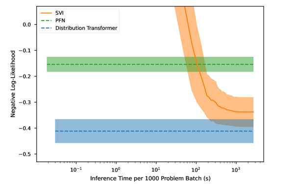
Figure 5: Expected negative log-likelihood against batch inference time for SVI, a PFN and a 5-component DT. Note that even given orders of magnitude more computation time, SVI cannot match the performance of our method, again demonstrating the power of our GMM approximation. Note that this problem is particularly challenging for VI, as the likelihood must be marginalized with respect to the uncertainty in the initial state and measurement time, which is not tractable and must be estimated stochastically, increasing the time per iteration.

Figure 5 illustrates the power of our approach, achieving better log-likelihood performance (and therefore a smaller KL-Divergence with the true posterior, indicating a better fit), than both competitor methods. This is a problem setting where variable priors are important, as they can be subjective in this setting, and prior sensitivity analysis can be important. To enable such an analysis, fast inference is also important. This illustrates the practical advantage of our approach over PFNs and VI well, as we explicitly target these problems.

4.3 Sequential Inference Study

The industry standard for real-time sequential inference (or Bayesian filtering), and therefore sensor fusion, is the Extended Kalman Filter (EKF). The EKF linearizes system dynamics and observation models, and approximates all sources of uncertainty as Gaussian. However, these assumptions are rarely reflected in reality. We tackle a sensor fusion problem consisting of 2-dimensional linear dynamics, modelled as a 4-dimensional state space (displacement and velocity), with indirect measurements of displacement provided by two independent, non-linear, non-Gaussian, sensors. Our approach is likely to be successful here, as prior time spent training is almost irrelevant, and fast inference with variable priors is the priority. We also validate against a particle filter, which handles these non-ideal conditions well at the expense of computation time.

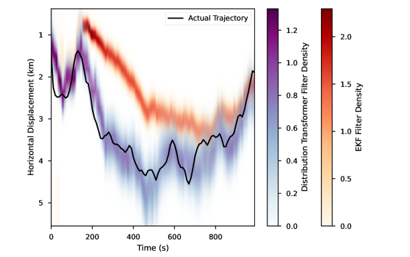
Figure 6: Marginal filter densities of horizontal displacement for both an EKF and a 4-component Distribution Transformer. Clearly, the DT tracks the true trajectory much more accurately, which is reflected in the superior expected NLL reported in Table 3. Note that the DT generally has a higher uncertainty than the EKF, demonstrating proper handling of the complex uncertainty structure of the observations.

Table 3: Expected NLL and iteration time (prediction, update and distribution generation) for EKF, PF, and DT. Note that our method vastly outperforms the EKF in terms of NLL with a small cost in iteration time, while almost matches the close to ground-truth PF’s NLL while achieving close to 50$\times$ speedup.

Method	Expected NLL	Iteration Time for 100 Series Batch (s)
EKF	95.9$\pm$4.40	0.010
PF	-0.244$\pm$0.047	0.818
DT	-0.197$\pm$0.040	0.017

Figure 6 clearly demonstrates that our approach tracks the true state well, while the EKF fails to track the true state at all. Table 3 confirms this, and shows that our approach sacrifices little in terms of iteration time, which upper bounds the frequency at which observations can be processed in real time, compared to the EKF. As expected, the close-to-ground truth PF achieves marginally better NLL than our method, at the expense of a significant slowdown.

5 Conclusion

In summary, Distribution Transformers (DTs) introduce a powerful framework for approximate Bayesian inference by combining universally-approximating Gaussian Mixture Models with Transformer architectures. Our empirical results demonstrate that DTs not only achieve superior inference accuracy and speed compared to existing methods, but also enable dynamic prior updates without retraining—a unique capability in the field. Furthermore, DTs show near-exact inference performance on challenging tasks including GP hyperposterior estimation, quantum parameter inference, and real-world sequential inference, while maintaining the computational efficiency needed for practical applications.

Impact Statement

This paper presents work whose goal is to advance the field of Machine Learning. There are many potential societal consequences of our work, none which we feel must be specifically highlighted here.

Appendix A Proof of Proposition 3.1

Proof.

This equality can shown with a simple derivation:

$$\ell_{\theta} =\mathbb{E}_{p(\phi,x,z)}\left[-\log q_{\theta}(f(x)\mathop{|}z,\phi)\right]$$

$$=\mathbb{E}_{p(\phi,z)}\left[\mathbb{E}_{p(x\mathop{|}\phi,z)}\left[-\log q_{\theta}(f(x)\mathop{|}z,\phi)\right]\right]$$

$$=\mathbb{E}_{p(\phi,z)}\left[\mathbb{E}_{p(x\mathop{|}\phi,z)}\left[-\log q_{\theta}(x\mathop{|}z,\phi)+\log\mathop{|}\det J_{f}(x)\mathop{|}\right]\right]$$

$$=\mathbb{E}_{p(\phi,z)}\left[\mathbb{E}_{p(x\mathop{|}\phi,z)}\left[\log p(x\mathop{|}z,\phi)-\log p(x\mathop{|}z,\phi)-\log q_{\theta}(x\mathop{|}z,\phi)+\log\mathop{|}\det J_{f}(x)\mathop{|}\right]\right]$$

$$=\mathbb{E}_{p(\phi,z)}\left[\mathbb{E}_{p(x\mathop{|}\phi,z)}\left[\log\frac{p(x\mathop{|}z,\phi)}{q_{\theta}(x\mathop{|}z,\phi)}\right]\right]+\mathbb{E}_{p(\phi,z)}\left[\mathbb{E}_{p(x\mathop{|}\phi,z)}\left[\log\mathop{|}\det J_{f}(x)\mathop{|}-\log p(x\mathop{|}z,\phi)\right]\right]$$

$$=\mathbb{E}_{p(\phi,z)}\left[\text{KL}\left[p(x\mathop{|}z,\phi)\mathop{||}q_{\theta}(x\mathop{|}z,\phi)\right]\right]+\mathbb{E}_{p(\phi,x,z)}\left[\log\mathop{|}\det J_{f}(x)\mathop{|}-\log p(x\mathop{|}z,\phi)\right],$$

where $J_{f}(x)$ denotes the Jacobian of $f(\cdot)$ evaluated at $x$, the third line follows from change of measure, and the term $\mathbb{E}_{p(\phi,x,z)}\left[\log\mathop{|}\det J_{f}(x)\mathop{|}-\log p(x\mathop{|}z,\phi)\right]$ is constant with respect to $\theta$. ∎

Appendix B General Architecture Details

Learnable prior embeddings typically consist of a multi-layer perceptron (MLP) with one hidden layer, usually of half the size of the transformer latent space. For GMM priors, the prior embedding acts elementwise and consists of a logarithm applied to the component weight, a Cholesky decomposition then logarithm of diagonal elements applied to the covariance matrix, and a flattening into a vector before passing through the MLP straight to the latent unordered sequence. For general priors, simple transformations are applied to parameters, for example positive parameters are passed through a logarithm, before being passed through the MLP to a single vector in the latent space. Then, distinct MLPs act on this vector to yield the components of the latent unordered sequence.

Learnable observation embeddings always consist only of an MLP, but theoretically could be extended to include inductive biases suitable for the nature of each observation. These embeddings are not processed further, and attend directly to the latent unordered sequence.

A standard transformer decoder setup is used, always consisting of 6 transformer decoder units, typically with a latent space size of 64, an MLP hidden layer size of 2048, and 8 attention heads.

The unembedding is almost an exact reverse to the GMM prior embedding, acting elementwise first with a learnable MLP, then the inverse of the Cholesky-log-flatten transform described earlier for the component covariance matrix. A cross-component softmax is then applied to the unembedded weight logits to yield the GMM.

Note that for numerical stability, GMMs were always parametrized directly by the Cholesky decomposition of the covariance matrix.

For PFNs, an identical setup was used wherever possible; Observations were embedded with the same embedding architecture, and the transformer encoder used identical hyperparameters to the DT for each experiment.

Appendix C General Training Details

All experiments were trained using the Adam optimizer without weight decay or dropout (overfitting here is impossible as the model sees each sample only once). A cosine-annealing-with-warmup (5 epochs) learning rate scheduler was used. This training scheme was adopted for both DTs and PFNs.

SVI also used the Adam optimizer without weight decay or dropout, treating the parameters of the variational distribution as model parameters, and directly optimizing the ELBO via backpropagation. An exponential learning rate scheduler was used.

Experiments 4.1, 4.2.2, and 4.3 were all carried out on an NVIDIA RTX 2080 Super laptop GPU (8GB VRAM), while experiment 4.2.1 was carried out on an NVIDIA RTX 3090 GPU.

Table 4: Training hyperparameters and statistics for all experiments. An epoch always consists of 100 batches. Hyperparameters were obtained by limited manual tuning, adjusted until training was stable in all cases. For SVI, the total samples reported account for batching, so the number of samples used by each SVI problem will be a factor of the number of test problems lesser. Parameters are listed vertically, corresponding to DTs (top), PFNs (middle), and SVI (bottom). For Experiment 4.1, only DT-5 is reported but training hyperparameters are identical for DT-2. For experiment 4.3 only DT is reported. For experiment 4.2.1, two PFNs are trained (one for each dimension, as PFNs do not trivially support multivariate distributions), so two figures are quoted when necessary (PPD + hyperposterior). Model sizes are not provided for VI as this is negligible.

Experiment	LR	Batch Size	Epochs	Total Samples (M)	Training Time (s)	Model Size (MB)
	0.005	5000	20	10	188	1.72
4.1	0.005	5000	20	10	247	1.16
	0.1	10	100	10	137	—
	0.0001	2000	200	40	4300	75.0
4.2.1	0.0001	1000	200+100	20+10	730+369	55.7
	0.03	10	1000	100	131	–
	0.001	5000	20	10	432	7.18
4.2.2	0.0001	4000	25	10	709	6.53
	0.01	10	100	10	2700	—
4.3	0.001	5000	150	75	3720	6.86

Appendix D Details for Analytical Verification Study (Experiment 4.1)

Here, for both the inverse-gamma prior’s rate and scale parameters, we adopt an $\text{InverseGamma}(4,6)$ meta-prior and an $\text{InverseGamma}(10000,20000)$ for the wide and narrow meta-priors respectively. Both of these meta-priors have the same mean, but the narrow meta-prior is effectively singular.

An analytical expression for the ground-truth posterior distribution is obtainable via conjugacy. Specifically, given a measurement $\sigma^{2}$ and prior parameters $\alpha_{0}$ and $\beta_{0}$, the parameters of the also inverse-gamma posterior are given by:

$$\alpha =\alpha_{0}+\frac{1}{2},\text{ and}$$

$$\beta =\beta_{0}+\frac{(z-\mu)^{2}}{2},$$

where $z$ is the observation value and $\mu$ is the known observation mean, which we arbitrarily set to 0.

Appendix E Details for Gaussian Process Joint PPD and Hyperposterior Study (Experiment 4.2.1)

For the meta prior in this experiment, we assign a narrow, uniform prior over the PPD’s prior such that it is marginally everywhere a standard normal. We assign a uniform prior on $[1,2]$ to both parameters of the inverse-gamma prior over lengthscale.

Note that for this experiment, the PPD prior also, in conjunction with the lengthscale $l$, defines the hyperparameters of the GP’s prior mean function and RBF covariance function used here. Specifically, the GP’s mean function is set to a constant at the PPD prior’s mean, and the output scale of the RBF covariance function is set to the standard deviation of the PPD’s prior.

The sampling procedure for this experiment, using 5 observations, was as follows:

1. Sample $\phi$ from meta-prior

2. Sample $y\sim\mathcal{N}(\phi_{\mu},\phi_{\sigma^{2}})$

3. Sample $l\sim\text{InverseGamma}(\phi_{\alpha},\phi_{\beta})$

4. Sample $x\sim\text{Uniform}(0,10)$

5. Sample $X\sim\text{Uniform}(0,10)^{5}$

6. Sample $Y\sim\mathcal{N}(\phi_{\mu},k(X,X;l,\phi_{\sigma^{2}}))$

7. Construct $z$ as concatenation of $X$ and $Y$ in the last dimension, along with the query point $x$.

Two observation embeddings are defined, one acting on each $X$-$Y$ element pair, and one acting on the query point $x$. Each have one hidden layer of size 128.

The prior embedding consists of two MLPs, acting on the PPD prior and the lengthscale prior respectively, each with one hidden layer of size 128, with 32 outputs. These outputs are concatenated into a single vector of size 64, before being passed through another set of distinct, parallel MLPs as before to yield the required length-10 latent unordered sequence.

Appendix F Details for Quantum System Parameter Inference Study (Experiment 4.2.2)

For this experiment, we adopt a beta prior, with an $\text{InverseGamma}(4,6)$ meta-prior over each parameter.

Observations are sampled using a GPU-implemented simulation, which accepts a nominal initial state $|{\hat{\psi}_{0}}\rangle$ and nominal measurement time $\hat{t}$. We model uncertainty in the initial state preparation by, treating $|{\hat{\psi}_{0}}\rangle$ as a 2-element vector, sampling an actual initial state $|{\psi_{0}}\rangle\sim\mathcal{N}(|{\hat{\psi}_{0}}\rangle,0.01I)$, and renormalizing such that $\langle{\psi_{0}}||{\psi_{0}}\rangle=1$. We also model uncertainty in measurement time by sampling $t\sim\mathcal{N}(\hat{t},0.0025)$. We then solve Schrödinger’s equation to give $|{\psi_{t}}\rangle$, and take a measurement by sampling from the Bernoulli distribution associated with $|{\psi_{t}}\rangle$. For SVI, the likelihood of this observation is estimated stochastically with 10 samples of the initial state and measurement time.

A set of varying nominal initial states and measurement times is fixed, and with each problem sampling an observation from each is obtained. Each pair of initial state and measurement time is provided its own learnable embedding, all of standard construction. The prior embedding and posterior unembedding is also standard.

Appendix G Details for Sequential Inference Study (Experiment 4.3)

For this experiment, we use the following meta-prior over a 4-component GMM:

$$w \sim\text{Dirichlet}(0.25\cdot\mathbf{1_{4}})$$

$$x_{i} \sim\mathcal{N}(\mathbf{0_{4}},4I_{4\times 4}) \forall i=1\ldots 4$$

$$\Sigma_{i} \sim\text{Wishart}(5,4I_{4\times 4}) \forall i=1\ldots 4,$$

where $\mathbf{1_{4}}$ and $\mathbf{0_{4}}$ refer to a 4-element vector consisting of only ones and zeros respectively.

We use two realistic observation models: A rangefinder subject to maximum range constraints, range-dependent Gaussian noise centred about the true range, exponentially distributed early measurements from unexpected objects, and uniformly distributed readings due to sensor failure, and bearing measurement subject to Gaussian noise and cyclic discontinuity (ie a wrapped normal distribution). Figure 7 demonstrates the complexity of the rangefinder observation model, and the parameters used in this experiment are presented in the caption.

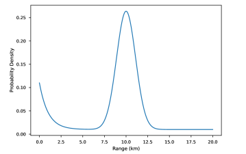
Figure 7: Example likelihood for rangefinder observation model, conditioned on a range of 10km. We assume a maximum range of 20km, a true observation standard deviation of $0.1(\text{range}+1)$km with marginal probability 0.7, an early collision decay rate of $1\text{km}^{-1}$ with marginal probability 0.2, and a uniform sensor failure on $\text{Uniform}(0,20\text{km})$ with marginal probability 0.1. While this model is realistic, the uncertainties involved are amplified compared to those seen in reality. This was done to further illustrate the capabilities of our model.

We report iteration time per 100 series. Concretely, this refers to the prediction, update, and density fitting, of a single time step batched across 100 series.

We use a motion model representing damped velocity subject to independent, normally distributed accelerations in each direction. Formally, we adopt the following discrete-time dynamical system:

$$x_{t+1} =\left[\begin{matrix}1&0.63&0&0\\ 0&0.37&0&0\\ 0&0&1&0.63\\ 0&0&0&0.37\end{matrix}\right]x_{t}+\left[\begin{matrix}0.1&0.0\\ 0.2&0.0\\ 0.0&0.1\\ 0.0&0.2\end{matrix}\right]w_{t}$$

$$w_{t} \sim\mathcal{N}(\mathbf{0_{2}},I_{2\times 2})$$

$$x_{0} \sim\mathcal{N}(\mathbf{1_{4}},I_{4\times 4})$$

References

- Bahdanau et al. (2014) Bahdanau, D., Cho, K., and Bengio, Y. Neural Machine Translation by Jointly Learning to Align and Translate. arXiv: Computation and Language, 2014.
- Binois & Wycoff (2021) Binois, M. and Wycoff, N. A Survey on High-dimensional Gaussian Process Modeling with Application to Bayesian Optimization. ACM Transactions on Evolutionary Learning and Optimization, 2021.
- Bishop (1994) Bishop, C. M. Mixture density networks. 1994.
- Bishop (2006) Bishop, C. M. Pattern Recognition and Machine Learning. Technometrics, 2006.
- Blei et al. (2016) Blei, D. M., Kucukelbir, A., and McAuliffe, J. Variational Inference: A Review for Statisticians. arXiv: Computation, 2016.
- Brooks et al. (2012) Brooks, S., Gelman, A., Jones, G. L., and Meng, X.-L. Handbook of Markov Chain Monte Carlo. Chance, 25:53–55, 2012.
- Brown et al. (2020) Brown, T. B., Mann, B., Ryder, N., Subbiah, M., Kaplan, J., Dhariwal, P., Neelakantan, A., Shyam, P., Sastry, G., Askell, A., Agarwal, S., Herbert-Voss, A., Krueger, G., Henighan, T., Child, R., Ramesh, A., Ziegler, D. M., Wu, J., Winter, C., Hesse, C., Chen, M., Sigler, E., Litwin, M., Gray, S., Chess, B., Clark, J., Berner, C., McCandlish, S., Radford, A., Sutskever, I., and Amodei, D. Language Models are Few-Shot Learners. Neural Information Processing Systems, 2020.
- Calcaterra & Boldt (2008) Calcaterra, C. and Boldt, A. Approximating with Gaussians. arXiv: Classical Analysis and ODEs, 2008.
- Christian & Casella (2011) Christian, R. R. and Casella, G. A Short History of MCMC: Subjective Recollections from Incomplete Data. Journal of machine learning research, pp. 75–92, 2011.
- Dempster et al. (1977) Dempster, A. P., Laird, N. M., and Rubin, D. B. Maximum likelihood from incomplete data via the EM algorithm. Journal of the royal statistical society series b-methodological, 39:1–22, 1977.
- Dosovitskiy et al. (2020) Dosovitskiy, A., Beyer, L., Kolesnikov, A., Weissenborn, D., Zhai, X., Unterthiner, T., Dehghani, M., Minderer, M., Heigold, G., Gelly, S., Uszkoreit, J., and Houlsby, N. An image is worth 16x16 words: Transformers for image recognition at scale. arXiv: Computer Vision and Pattern Recognition, 2020.
- Ganguly et al. (2023) Ganguly, A., Jain, S., and Watchareeruetai, U. Amortized Variational Inference: A Systematic Review. Journal of Artificial Intelligence Research, 78:167–215, 2023.
- Gawlikowski et al. (2021) Gawlikowski, J., Tassi, C. R. N., Ali, M., Lee, J., Humt, M., Feng, J., Kruspe, A. M., Triebel, R., Jung, P., Roscher, R., Shahzad, M., Yang, W., Bamler, R., and Zhu, X. A survey of uncertainty in deep neural networks. Artificial Intelligence Review, 2021.
- Goodfellow et al. (2016) Goodfellow, I., Bengio, Y., and Courville, A. Deep Learning. MIT Press, 2016.
- Hoffman & Gelman (2011) Hoffman, M. and Gelman, A. The No-U-turn sampler: adaptively setting path lengths in Hamiltonian Monte Carlo. Journal of machine learning research, 2011.
- Hoffman et al. (2013) Hoffman, M. D., Blei, D. M., Wang, C., and Paisley, J. Stochastic variational inference. Journal of Machine Learning Research, 14:1303–1347, 2013.
- Hüllermeier & Waegeman (2019) Hüllermeier, E. and Waegeman, W. Aleatoric and Epistemic Uncertainty in Machine Learning: An Introduction to Concepts and Methods. arXiv: Learning, 2019.
- Julier & Uhlmann (1997) Julier, S. J. and Uhlmann, J. K. New extension of the kalman filter to nonlinear systems. In Defense, Security, and Sensing, 1997. URL https://api.semanticscholar.org/CorpusID:7937456.
- Kingma & Welling (2014) Kingma, D. P. and Welling, M. Auto-Encoding Variational Bayes. International Conference on Learning Representations, 2014.
- LeCun et al. (2015) LeCun, Y., Bengio, Y., and Hinton, G. E. Deep learning. Nature, 521:436–444, 2015.
- Minka (2001) Minka, T. Expectation propagation for approximate Bayesian inference. Conference on Uncertainty in Artificial Intelligence, pp. 362–369, 2001.
- Muller et al. (2021) Muller, S., Hollmann, N., Pineda Arango, S., Grabocka, J., and Hutter, F. Transformers Can Do Bayesian Inference. International Conference on Learning Representations, 2021.
- Osborne et al. (2012) Osborne, M. A., Garnett, R., Ghahramani, Z., Duvenaud, D., Roberts, S. J., and Rasmussen, C. E. Active Learning of Model Evidence Using Bayesian Quadrature. Neural Information Processing Systems, 25, 2012.
- Paszke et al. (2019) Paszke, A., Gross, S., Massa, F., Lerer, A., Bradbury, J., Chanan, G., Killeen, T., Lin, Z., Gimelshein, N., Antiga, L., Desmaison, A., Kopf, A., Yang, E., DeVito, Z., Raison, M., Tejani, A., Chilamkurthy, S., Steiner, B., Fang, L., Bai, J., and Chintala, S. PyTorch: An Imperative Style, High-Performance Deep Learning Library. Neural Information Processing Systems, 32:8026–8037, 2019.
- Ranganath et al. (2014) Ranganath, R., Gerrish, S., and Blei, D. M. black box variational inference. Journal of Machine Learning Research, 2014.
- Rezende & Mohamed (2015) Rezende, D. J. and Mohamed, S. Variational Inference with Normalizing Flows. arXiv: Machine Learning, 2015.
- Tierney & Kadane (1986) Tierney, L. and Kadane, J. B. Accurate Approximations for Posterior Moments and Marginal Densities. Journal of the American Statistical Association, 81:82–86, 1986.
- Vaswani et al. (2017) Vaswani, A., Shazeer, N., Parmar, N., Uszkoreit, J., Jones, L., Gomez, A. N., Kaiser, L., and Polosukhin, I. Attention is All you Need. Neural Information Processing Systems, 30:5998–6008, 2017.
- Wills & Schön (2023) Wills, A. and Schön, T. B. Sequential Monte Carlo: A Unified Review. Annu. Rev. Control. Robotics Auton. Syst., 6:159–182, 2023.
- Yun et al. (2019) Yun, C., Bhojanapalli, S., Rawat, A. S., Reddi, S. J., and Kumar, S. Are Transformers universal approximators of sequence-to-sequence functions? arXiv: Learning, 2019.