Robust and Conjugate Spatio-Temporal Gaussian Processes

Abstract

State-space formulations allow for Gaussian process (GP) regression with linear-in-time computational cost in spatio-temporal settings, but performance typically suffers in the presence of outliers. In this paper, we adapt and specialise the robust and conjugate GP (RCGP) framework of Altamirano et al. (2024) to the spatio-temporal setting. In doing so, we obtain an outlier-robust spatio-temporal GP with a computational cost comparable to classical spatio-temporal GPs. We also overcome the three main drawbacks of RCGPs: their unreliable performance when the prior mean is chosen poorly, their lack of reliable uncertainty quantification, and the need to carefully select a hyperparameter by hand. We study our method extensively in finance and weather forecasting applications, demonstrating that it provides a reliable approach to spatio-temporal modelling in the presence of outliers.

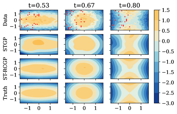
Figure 1: Spatio-temporal GPs in the presence of outliers. The top row shows the observed data as a function of spatial covariates $\mathbf{s}\in\mathbb{R}^{2}$. Outliers are highlighted in red and are uniformly distributed on $[-8,-6]\cup[6,8]$. The second row gives the fit of a regular STGP, whilst the third row gives our proposed ST-RCGP fit. The last row shows the true latent function $f(s_{1},s_{2},t)=\sin(2\pi t)s_{1}^{2}+\cos(2\pi t)s_{2}^{2}$. Further details are provided in Section C.4.

1 Introduction

Gaussian processes (GPs; Williams and Rasmussen, 2006) are flexible probabilistic models used in a vast class of problems from regression (Williams and Rasmussen, 2006) to emulation (Santner et al., 2018) and optimisation (Garnett, 2023). GPs originated in spatial statistics, where their use for regression was known as kriging (Krige, 1951; Stein, 1999), but they have more recently been used widely in spatio-temporal settings, including in epidemiology (Senanayake et al., 2016), neuroimaging (Hyun et al., 2016), object tracking (Aftab et al., 2019), and psychological studies (Kupilik and Witmer, 2018). Their popularity arises from their ability to encode spatial and temporal properties such as smoothness, periodicity, and sparsity (Duvenaud, 2014), allowing to model phenomena such as local weather patterns or seasonality. Crucially, GPs also have an exact, closed-form posterior when using a Gaussian likelihood. However, naive implementations have a cubic computational cost in the number of data points $N$, limiting their scalability. To address this issue, a plethora of approximations have been proposed (Drineas et al., 2005; Titsias, 2009; Hensman et al., 2013; Wilson and Nickisch, 2015). While effective, these do not typically recover the exact GP, require careful tuning, and can degrade performance for complex datasets (Bauer et al., 2016; Pleiss et al., 2018).

In spatio-temporal settings, an alternative strategy is to reformulate the GP as a state-space model (SSM) (Reece and Roberts, 2010; Hartikainen and Särkkä, 2010; Sarkka and Hartikainen, 2012; Solin, 2016; Nickisch et al., 2018; Hamelijnck et al., 2021). This gives rise to a class of models—spatio-temporal Gaussian processes (STGPs)—with linear cost in the number of temporal observations. But, as with standard GPs, STGPs lack robustness to model misspecification, such as with outliers arising from extreme events (Heaton et al., 2011), measurement errors that are spatially correlated (Tadayon and Rasekh, 2019), and other heterogeneities (Fonseca et al., 2023). Figure 1 illustrates this in the case of outliers. Clearly, the STGP ($2^{\text{nd}}$ row) fails to align with the ground truth ($4^{\text{th}}$ row).

To resolve this issue, existing work on STGPs has focused on using likelihoods corresponding to distributions which are more expressive than Gaussians, such as mixtures or heavy-tailed distributions. Doing so breaks conjugacy, and the posterior must typically be approximated (Hartikainen et al., 2011; Solin and Särkkä, 2014; Hamelijnck et al., 2021). We refer the reader to Nickisch et al. (2018) for a comprehensive overview and to Wilkinson et al. (2023) for a Python package providing those algorithms. Although these methods have been efficiently implemented, they typically use additional optimisation steps at each time-point and are hence significantly more costly than conjugate STGPs.

Recently, Altamirano et al. (2024) introduced a method, called robust and conjugate Gaussian processes (RCGPs), that uses generalised Bayesian inference (Bissiri et al., 2016; Knoblauch et al., 2022) to confer robustness to standard GPs. Their approach is highly attractive since it provably provides robustness to outliers whilst maintaining conjugacy, but it shares the cubic cost of GPs. Existing work on RCGPs also has three main limitations: RCGPs underperform when the prior mean is chosen poorly (see Ament et al. (2024) and the Appendix of Altamirano et al. (2024)), their uncertainty quantification properties have not been well-studied, and they have an additional hyperparameter compared to standard GPs. Further, the existing heuristic for tuning this parameter relates to the proportion of outliers in the data, which is unknown in practice and generally has to be hand-picked on a case-by-case basis.

In this paper, we show how to refine and specialise the RCGP framework for spatio-temporal data. Our algorithm, denoted spatio-temporal RCGP (ST-RCGP), inherits the computational and memory efficiency of STGPs, as well as the robustness properties of RCGPs (see $3^{\text{rd}}$ row of Figure 1). The sequential aspect of the state-space formulation also allows us to overcome the three main limitations of RCGPs (sensitivity to prior mean, lack of reliable uncertainty quantification, and additional hyperparameter). Overall, we observe that ST-RCGPs provide inferences that are comparable to state-of-the-art non-Gaussian STGPs in the presence of outliers, but at a fraction of the cost.

2 Background

GP Regression

Let $\{\mathbf{x}_{k},y_{k}\}_{k=1}^{N}$ be observations, where $\mathbf{x}_{k}\in\mathcal{X}\subseteq\mathbb{R}^{d}$ are covariates and $y_{k}\in\mathcal{Y}\subseteq\mathbb{R}$ are responses. For observation noise $\epsilon_{k}$, GP regression considers

$$y_{k}=f(\mathbf{x}_{k})+\epsilon_{k},\quad\text{for }k=1,\ldots,N$$ (1)

where the latent function $f:\mathcal{X}\rightarrow\mathbb{R}$ is modelled by a GP prior $f\sim\mathcal{GP}(m,\kappa)$ with mean $m:\mathcal{X}\rightarrow\mathbb{R}$ and covariance (or kernel) $\kappa:\mathcal{X}\times\mathcal{X}\rightarrow\mathbb{R}$, such that for any inputs $\mathbf{X}=(\mathbf{x}_{1},...,\mathbf{x}_{N})^{\top}$, the vector $\mathbf{f}=(f(\mathbf{x}_{1}),...,f(\mathbf{x}_{N}))^{\top}$ is distributed as a $N$-dimensional Gaussian $\mathcal{N}(\mathbf{m},\mathbf{K})$ with $\mathbf{m}=(m(\mathbf{x}_{1}),...,m(\mathbf{x}_{N}))^{\top}$ and $(\mathbf{K})_{ij}=\kappa(\mathbf{x}_{i},\mathbf{x}_{j})$. The kernel $\kappa$ typically depends on parameters $\bm{\theta}\in\Theta$ that we omit from the notation for brevity. When the observations $\mathbf{y}=(y_{1},...,y_{N})^{\top}$ have independent Gaussian noise $(\epsilon_{1},\ldots,\epsilon_{N})^{\top}\sim\mathcal{N}(0,\sigma^{2}\mathbf{I}_{N})$, the posterior predictive for $f_{\star}=f(x_{\star})$ at $x_{\star}\in\mathcal{X}$ is $f_{\star}|\mathbf{y},\mathbf{X}\sim\mathcal{N}(\mu_{\text{GP}}^{\star},\Sigma_{\text{GP}}^{\star})$ with

$$\begin{split}&\mu_{\text{GP}}^{\star}=m_{\star}+\mathbf{k}_{\star}^{\top}\left(\mathbf{K}+\sigma^{2}{\color[rgb]{1,0.49,0}\mathbf{I}_{N}}\right)^{-1}\left(\mathbf{y}-{\color[rgb]{1,0.49,0}\mathbf{m}}\right)\\ &\Sigma_{\text{GP}}^{\star}=k_{\star\star}-\mathbf{k}_{\star}^{\top}(\mathbf{K}+\sigma^{2}{\color[rgb]{1,0.49,0}\mathbf{I}_{N}})^{-1}\mathbf{k}_{\star}\end{split}$$ (2)

where $\mathbf{I}_{N}$ is the $N\times N$ identity matrix, $\mathbf{k}_{\star}=(\kappa(x_{\star},x_{1}),...,\kappa(x_{\star},x_{N}))^{\top}$, $k_{\star\star}=\kappa(x_{\star},x_{\star})$, and $m_{\star}=m(x_{\star})$. The orange colouring can be ignored for now, but will be used to highlight differences with RCGPs. To obtain this mean and covariance, we must invert an $N\times N$ matrix—an operation with computational complexity $\mathcal{O}(N^{3})$.

State-Space Formulation

An alternative approach which provides $\mathcal{O}(N)$ cost is to use a state-space representation. Consider (1) with spatio-temporal inputs. At time $t_{k}\in\mathcal{T}\subseteq\mathbb{R}$, we now have inputs $\mathbf{x}_{k,j}=(\mathbf{s}_{j},t_{k})\in\mathcal{X}=\mathcal{S}\times\mathcal{T}$ on a spatial grid $\mathbf{S}=(\mathbf{s}_{1},\ldots,\mathbf{s}_{n_{s}})^{\top}\in\mathcal{S}^{n_{s}}\subseteq\mathbb{R}^{n_{s}\times d_{s}}$ with $n_{s}$ points and spatial dimensionality $d_{s}$ (i.e. $d=d_{s}+1$). The observations corresponding to $\mathbf{x}_{k}=(\mathbf{x}_{k,1},\ldots,\mathbf{x}_{k,n_{s}})^{\top}$ are denoted $\mathbf{y}_{k}=(y_{k,1},\ldots,y_{k,n_{s}})^{\top}\in\mathbb{R}^{n_{s}}$, leading to a total number of data points $N=n_{t}n_{s}$ where $n_{t}$ is the number of time steps. If standard GPs were used here, the cost would be $\mathcal{O}(n_{t}^{3}n_{s}^{3})$, which would be impractical.

A solution to this issue is to reformulate GPs as SSMs. We first collect $\nu$ partial derivatives of $f$ with respect to time in a state vector $\mathbf{z}=\mathbf{z}(\mathbf{s},t)\in\mathbb{R}^{(\nu+1)}$ where $(\mathbf{z}(\mathbf{s},t))_{i}=\frac{\partial^{i-1}}{\partial t^{i-1}}f(\mathbf{s},t)$ for $i=1,...,\nu+1$. Assuming a stationary and separable kernel so that $\kappa(\mathbf{s},t;\mathbf{s}^{\prime},t^{\prime})=\kappa_{s}(\mathbf{s}-\mathbf{s}^{\prime})\kappa_{t}(t-t^{\prime})$, where $\kappa_{s}$ and $\kappa_{t}$ are spatial and temporal kernels respectively, we can represent the GP prior as the solution to a stochastic differential equation (SDE):

$$\begin{split}\frac{\partial\mathbf{z}(\mathbf{s},t)}{\partial t}=\mathbf{F}_{t}\mathbf{z}(\mathbf{s},t)+\mathbf{L}_{t}\mathbf{w}(\mathbf{s},t),\end{split}$$ (3)

where $\mathbf{F}_{t}\in\mathbb{R}^{(\nu+1)\times(\nu+1)}$, $\mathbf{L}_{t}\in\mathbb{R}^{(\nu+1)\times 1}$, and $\mathbf{w}(\mathbf{s},t)$ is a spatio-temporal white noise process corresponding to the derivative of Brownian motion with spectral density $\mathbf{Q}_{c,t}\in\mathbb{R}^{1\times(\nu+1)}$ (Solin, 2016). The matrices $\mathbf{F}_{t}$, $\mathbf{L}_{t}$, $\mathbf{Q}_{c,t}$ and the constant $\nu$ depend on $\kappa$.

Equation 3 defines a continuous latent process, but given a finite collection of points, this becomes a SSM with states $\mathbf{z}_{k}=(\mathbf{z}(\mathbf{s}_{1},t_{k}),...,\mathbf{z}(\mathbf{s}_{n_{s}},t_{k}))^{\top}\in\mathbb{R}^{n_{s}(\nu+1)}$ and time steps $\Delta t_{k}=t_{k}-t_{k-1}$ (Hartikainen and Särkkä, 2010; Sarkka and Hartikainen, 2012; Särkkä and Solin, 2019):

$$\begin{split}&\mathbf{z}_{0}\sim\mathcal{N}(\mathbf{0},\mathbf{\Sigma}_{0}),\;\text{and for}\;k>0,\\ &\mathbf{z}_{k}=\mathbf{A}_{k-1}\mathbf{z}_{k-1}+\mathbf{q}_{k-1},\quad\mathbf{q}_{k-1}\sim\mathcal{N}(\mathbf{0},\mathbf{\Sigma}_{k-1})\\ &\mathbf{y}_{k}=\mathbf{H}\mathbf{z}_{k}+\mathbf{\epsilon}_{k}\end{split}$$ (4)

where $\mathbf{H}\in\mathbb{R}^{n_{s}\times n_{s}(\nu+1)}$ is defined such that $\mathbf{H}\mathbf{z}_{k}=\mathbf{f}_{k}:=\left(f(\mathbf{s}_{1},t_{k}),...,f(\mathbf{s}_{n_{s}},t_{k})\right)^{\top}$. The matrices $\mathbf{A}_{k-1}$ and $\mathbf{\Sigma}_{k-1}$ depend on $\mathbf{F}_{t}$, $\mathbf{L}_{t}$ and $\mathbf{Q}_{c,t}$ in the SDE formulation. We define them in Section C.2, and provide information on how to compute them in practice for a list of common kernels $\kappa$.

Filtering and Smoothing

Solving the SSM from (4) via sequential inference amounts to first retrieving the filtering distribution $p(\mathbf{z}_{k}|\mathbf{y}_{1:k})$, and then the smoothing distribution $p(\mathbf{z}_{k}|\mathbf{y}_{1:N})$ (Särkkä, 2013). Taking (4), and assuming the observation noise is Gaussian so that $\epsilon_{k}\sim\mathcal{N}(0,\sigma^{2}\mathbf{I}_{n_{s}(\nu+1)})$, the predict and update equations are conjugate and given by the Kalman filter (Kalman, 1960) and Rauch-Tung-Striebel smoother (Rauch et al., 1965); see Section 8.2 of Särkkä (2013). The resulting distribution has densities $p(\mathbf{z}_{k}|\mathbf{y}_{1:k-1})=\mathcal{N}(\mathbf{z}_{k};\mathbf{m}_{k|k-1},\mathbf{P}_{k|k-1})$ and $p(\mathbf{z}_{k}|\mathbf{y}_{1:k})=\mathcal{N}(\mathbf{z}_{k};\mathbf{m}_{k|k},\mathbf{P}_{k|k})$, with predict step:

$$\begin{split}&\mathbf{m}_{k|k-1}:=\mathbf{A}_{k-1}\mathbf{m}_{k-1|k-1}\\ &\mathbf{P}_{k|k-1}:=\mathbf{A}_{k-1}\mathbf{P}_{k-1|k-1}\mathbf{A}_{k-1}^{\top}+\mathbf{\Sigma}_{k-1},\end{split}$$ (5)

and (Bayes) update step:

$$\begin{split}&\mathbf{P}_{k|k}:=\left(\mathbf{P}_{k|k-1}^{-1}+\mathbf{H}^{\top}\sigma^{-2}{\color[rgb]{0,1,0}\mathbf{I}_{n_{s}(\nu+1)}}\mathbf{H}\right)^{-1}\\ &\mathbf{K}_{k}:=\mathbf{P}_{k|k}\mathbf{H}^{\top}\sigma^{-2}{\color[rgb]{0,1,0}\mathbf{I}_{n_{s}(\nu+1)}}\\ &\mathbf{m}_{k|k}:=\mathbf{m}_{k|k-1}+\mathbf{K}_{k}(\mathbf{y}_{k}-{\color[rgb]{0,1,0}\hat{\mathbf{f}}_{k}}),\end{split}$$ (6)

where $\hat{\mathbf{f}}_{k}:=\mathbf{H}\mathbf{m}_{k|k-1}$, $\mathbf{K}_{k}\in\mathbb{R}^{n_{s}(\nu+1)\times n_{s}}$, $\mathbf{m}_{k|k}\in\mathbb{R}^{n_{s}(\nu+1)}$ and $\mathbf{P}_{k|k}\in\mathbb{R}^{n_{s}(\nu+1)\times n_{s}(\nu+1)}$. The posterior $p(\mathbf{z}_{k}|\mathbf{y}_{1:N})$ is obtained by marginalising the smoothing distribution, and matches exactly the original GP posterior (Solin, 2016). For a new input $(\mathbf{s}_{\star},t_{\star})$, the predictive is obtained by including $(\mathbf{s}_{\star},t_{\star})$ in the filtering and smoothing algorithms and predicting without updating. Importantly, this algorithm only inverts matrices whose sizes scale with $\nu$—where typically $\nu<10$ (Hartikainen and Särkkä, 2010)—or $n_{s}$, but not with $n_{t}$. In contrast to the standard GP’s $\mathcal{O}(n_{t}^{3}n_{s}^{3})$ time and $\mathcal{O}(n_{t}^{2}n_{s}^{2})$ memory cost, the STGP only requires $\mathcal{O}(n_{t}n_{s}^{3})$ time and $\mathcal{O}(n_{t}n_{s}^{2})$ memory (Solin, 2016).

Figure 2: Behaviour of $y\mapsto w_{\text{IMQ}}(\mathbf{x}_{k},y)$ as we vary $c$, $\beta$, and $\gamma$. We emphasize $|y_{k}-\gamma(\mathbf{x}_{k})|$ and $w_{\text{IMQ}}(\mathbf{x}_{k},y_{k})$ with datum $y_{k}$.

Generalised Bayes for GP Regression

Conjugate GPs and STGPs rely on the fragile assumption that $\epsilon_{1},\ldots,\epsilon_{N}$ are Gaussian. While non-Gaussian likelihoods can address this, they also break conjugacy—and thus require expensive and potentially inaccurate approximations. Fortunately, generalised Bayes (GB) (Bissiri et al., 2016; Knoblauch et al., 2022) can produce robust and conjugate GP posteriors. GB mitigates model misspecification by constructing posterior distributions through a loss $\mathcal{L}:\mathcal{Y}^{N}\times\mathcal{Y}^{N}\times\mathcal{X}^{N}\rightarrow\mathbb{R}$ via

$$p_{\mathcal{L}}(\mathbf{f}|\mathbf{X},\mathbf{y})\propto p(\mathbf{f}|\mathbf{X})\exp\left(-N\mathcal{L}(\mathbf{y};\mathbf{f},\mathbf{X})\right),$$ (7)

where $\propto$ denotes proportionality and $\mathcal{L}$ is typically an estimator of a statistical divergence between the likelihood model and the data (Jewson et al., 2018). The loss $\mathcal{L}$ used for RCGPs (Altamirano et al., 2024) is a modification of the weighted score-matching divergence, first proposed by Barp et al. (2019), to regression. It generalises score-matching (Hyvärinen, 2005), and is a special case of the framework in Lyu (2009); Yu et al. (2019); Xu et al. (2022). Importantly, it uses a weight function $w:\mathcal{X}\times\mathcal{Y}\rightarrow\mathbb{R}\setminus\{0\}$ that down-weights unreasonably extreme data points. This choice yields the RCGP posterior predictive $f_{\star}\sim\mathcal{N}(\mu_{\text{RCGP}}^{\star},\Sigma_{\text{RCGP}}^{\star})$ with

$$\begin{split}&\mu_{\text{RCGP}}^{\star}=m_{\star}+\mathbf{k}_{\star}^{\top}\left(\mathbf{K}+\sigma^{2}{\color[rgb]{1,0.49,0}\mathbf{J}_{\mathbf{w}}}\right)^{-1}\left(\mathbf{y}-{\color[rgb]{1,0.49,0}\mathbf{m}_{\mathbf{w}}}\right)\\ &\Sigma_{\text{RCGP}}^{\star}=k_{\star\star}-\mathbf{k}_{\star}^{\top}(\mathbf{K}+\sigma^{2}{\color[rgb]{1,.5,0}\mathbf{J}_{\mathbf{w}}})^{-1}\mathbf{k}_{\star},\end{split}$$ (8)

where $\mathbf{w}=(w(\mathbf{x}_{1},y_{1}),...,w(\mathbf{x}_{N},y_{N}))^{\top}$, $\mathbf{m}_{\mathbf{w}}=\mathbf{m}+\sigma^{2}\nabla_{y}\log(\mathbf{w}^{2})$, and $\mathbf{J}_{\mathbf{w}}=\text{diag}(\frac{\sigma^{2}}{2}\mathbf{w}^{-2})$. The expressions look similar to those in (2), with differences highlighted in orange. This also reveals that standard GPs are recovered for the constant weight $w(\mathbf{x},y)=\sigma/\sqrt{2}$. The similar forms also suggest that much like classical GPs, a naive implementation of RCGPs has a complexity of $\mathcal{O}(N^{3})$ due to the associated matrix inversion. However, under mild conditions on $w$, RCGPs benefit from provable robustness to outliers (see Proposition 3.2 of Altamirano et al., 2024).

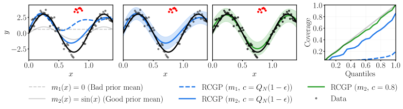
Figure 3: Failure Modes with Existings RCGPs. We generated $N=80$ data points from the true function $f(x)=3\sin(2\pi x)$ using $\mathcal{N}(0,0.5)$ additive noise, then corrupted $\epsilon=10\%$ of observations around $x=0.76$. The leftmost figure shows that RCGP’s posterior mean is strongly affected by the choice of prior mean, highlighting Issue #1. In the two middle plots, we demonstrate that the recommended $c=Q_{N}(1-\epsilon)=3.7$ (from Altamirano et al. (2024)) is far from optimal—emphasizing Issue #3—even when fitting simple data and knowing the true proportion of outliers $\epsilon$. These two plots also show RCGP’s inaccurate uncertainty quantification when hyperparameters are chosen poorly, which is further supported by the rightmost coverage plot and illustrates Issue #2.

In prior work, Altamirano et al. (2024) suggested to take $w$ of the form of an inverse multi-quadric (IMQ) kernel depending on a centering function $\gamma:\mathcal{X}\rightarrow\mathbb{R}$, a shrinking function $c:\mathcal{X}\rightarrow\mathbb{R}$, and a constant $\beta>0$:

$$w_{\text{IMQ}}(\mathbf{x},y)=\beta\left(1+\frac{(y-\gamma(\mathbf{x}))^{2}}{c(\mathbf{x})^{2}}\right)^{-\frac{1}{2}}$$ (9)

The IMQ has been used frequently to robustify score-based divergences (Barp et al., 2019; Key et al., 2021; Matsubara et al., 2022; Altamirano et al., 2023; Matsubara et al., 2024; Liu and Briol, 2024). It is a bump function centred at $\gamma(\mathbf{x})$ that grows as $|y-\gamma(\mathbf{x})|$ decreases, and shrinks as $|y-\gamma(\mathbf{x})|$ increases (see Figure 2). The centering function $\gamma(\mathbf{x})$ determines where the bump is maximised, and any $y$ far from $\gamma(\mathbf{x})$ is downweighted (see Figure 2). The shrinking function $c(\mathbf{x})$ determines how quickly we downweight observations that deviate from $\gamma(\mathbf{x})$, and $\beta$ determines the maximum of the weight function (see Figure 2). Note that $\beta$ is a multiplicative constant which is equivalent to a GB learning rate (Wu and Martin, 2023).

While the IMQ-based weights have shown much promise, they rely on three hyperparameters: $\gamma$, $\beta$, and $c$. Altamirano et al. (2024) proposed centering at the prior mean via $\gamma(\mathbf{x})=m(\mathbf{x})$, and setting $\beta=\sigma/\sqrt{2}$ to guarantee that observations are never assigned a larger weight than they would in a standard GP. Finally, they suggested a heuristic choice for $c$ based on the assumed proportion of outliers: if $\epsilon\in[0,1]$ is the expected proportion of outliers, they suggest setting the shrinking function to the constant $c(\mathbf{x})=Q_{N}(1-\epsilon)$, for $Q_{N}(1-\epsilon)$ the $(1-\epsilon)^{\text{th}}$ quantile of $\{|y_{k}-\gamma(\mathbf{x}_{k})|\}_{k=1}^{N}$. While these choices provide good performance in many settings, there are several failure modes:

• Issue #1 (Sensitivity to the prior mean $m$): Altamirano et al. (2024); Ament et al. (2024) pointed to the poor performance of RCGPs when $m$ is not chosen carefully. Indeed, setting $\gamma(\mathbf{x}):=m(\mathbf{x})$ can be undesirable when $m$ is not a good approximation of $f$. In that case, observations close to $m(\mathbf{x})$ but far from $f(\mathbf{x})$ will have large weights despite likely being outliers, whereas observations close to $f(\mathbf{x})$ but far from $m(\mathbf{x})$ will be down-weighted despite likely having little noise. We show this in Figure 3. Altamirano et al. (2024) suggest fixing this problem by choosing a prior mean using a simpler regression model, but this solution requires an additional fit of the data, which can be cumbersome.

• Issue #2 (Poor uncertainty quantification): The values of $\beta$ and $c$ have a significant influence on the predictive variance, but it is not clear that the suggested choices are sensible when it comes to uncertainty quantification and Altamirano et al. (2024) did not study this question. This could mean that RCGPs are consistently under- or over-confident—a problem we also illustrate in Figure 3. Sinaga et al. (2024) proposed a computation-aware extension of RCGPs to improve uncertainty quantification, but their approach still depends on having good values for $\beta$ and $c$.

• Issue #3 (Selection of shrinking function $c$): The proposed heuristic for selecting $c$ requires the user to speculate on the proportion $\epsilon$ of outliers. Not only is this hard to do reliably if we do not know $\epsilon$ but, as shown in Figure 3, the approach can also fail to select good values of $c$ even when the correct $\epsilon$ is used. This can lead to unreliable posterior estimates, and either under- or over-confidence of the RCGP posterior. In addition, setting $\mathbf{x}\mapsto c(\mathbf{x})$ to be constant can be sub-optimal when outliers are clustered in time or space, in which case adapting the shrinking function according to its input could lead to improved uncertainty quantification.

3 Methodology

Spatio-Temporal RCGPs

We now show that, similarly to GPs, inference for RCGPs can be performed using an SSM representation and filtering/smoothing updates.

Proposition 3.1.

Suppose we model $\epsilon_{1},\ldots,\epsilon_{N}\sim\mathcal{N}(0,\sigma^{2})$ and choose $w:\mathcal{X}\times\mathcal{Y}\rightarrow\mathbb{R}\setminus\{0\}$ such that $y\mapsto w(y,x)$ is differentiable. Then, we obtain a (generalised) posterior $p_{\mathcal{L}}(\mathbf{z}_{k}|\mathbf{y}_{1:k})=\mathcal{N}(\mathbf{z}_{k};\mathbf{m}^{\text{GB}}_{k|k},\mathbf{P}_{k|k}^{\text{GB}})$ and can perform sequential inference on the SSM formulation of RCGPs with predict step:

$$\begin{split}&\mathbf{m}_{k|k-1}:=\mathbf{A}_{k-1}\mathbf{m}^{\text{GB}}_{k-1|k-1}\\ &\mathbf{P}_{k|k-1}:=\mathbf{A}_{k-1}\mathbf{P}^{\text{GB}}_{k-1|k-1}\mathbf{A}_{k-1}^{\top}+\mathbf{\Sigma}_{k-1},\\ \end{split}$$

and (generalised Bayes) update step:

$$\begin{split}&\mathbf{P}_{k|k}^{\text{GB}}:=\left(\mathbf{P}_{k|k-1}^{-1}+\mathbf{H}^{\top}\sigma^{-2}{\color[rgb]{0,1,0}\mathbf{J}_{\mathbf{w}_{k}}^{-1}}\mathbf{H}\right)^{-1}\\ &\mathbf{K}_{k}^{\text{GB}}:=\mathbf{P}_{k|k}^{\text{GB}}\mathbf{H}^{\top}\sigma^{-2}{\color[rgb]{0,1,0}\mathbf{J}_{\mathbf{w}_{k}}^{-1}}\\ &\mathbf{m}_{k|k}^{\text{GB}}:=\mathbf{m}_{k|k-1}+\mathbf{K}_{k}^{\text{GB}}(\mathbf{y}_{k}-{\color[rgb]{0,1,0}\hat{\mathbf{f}}_{w_{k}}}),\end{split}$$

for $\hat{\mathbf{f}}_{w_{k}}:=\hat{\mathbf{f}}_{k}+\sigma^{2}\nabla_{y}\log(\mathbf{w}_{k}^{2})$, $\mathbf{J}_{\mathbf{w}_{k}}=\text{diag}(\frac{\sigma^{2}}{2}\mathbf{w}^{-2}_{k})$. Moreover, the GB predictive is $p_{\mathcal{L}}(\mathbf{y}_{k}|\mathbf{y}_{1:k-1})=\mathcal{N}(\mathbf{y}_{k};\hat{\mathbf{f}}_{k},\hat{\mathbf{S}}_{k})$ for $\hat{\mathbf{S}}_{k}:=\mathbf{H}\mathbf{P}_{k|k-1}\mathbf{H}^{\top}+\sigma^{2}\mathbf{I}_{n_{s}}$.

We refer to the SSM formulation of RCGPs as ST-RCGPs, and note that the above closely relates to existing GB filtering updates (Duran-Martin et al., 2024; Reimann, 2024). This proposition offers two key advantages: (1) we operate with significantly smaller matrices of size $n_{s}(\nu+1)\times n_{s}(\nu+1)$ instead of $n_{t}n_{s}\times n_{t}n_{s}$ for RCGPs, improving computational efficiency while maintaining robustness and conjugacy; and (2) whilst RCGPs require the weight function to be fixed during inference, we can adapt it as filtering is performed. This is reflected in our notation, which now indexes the weights with time. This last feature will allow us to address Issues #1, #2, and #3 mentioned in Section 2.

Weight Function

Despite the fact that the proof of robustness in Proposition 3.2 of Altamirano et al. (2024) and our Proposition 3.1 only have mild requirements on $w$, we found that using $w:=w_{\text{IMQ}}$ is desirable since it strikes a favourable balance between robustness to outliers and statistical efficiency in well-specified settings. To select $\gamma,\beta$ and $c$, we follow four guiding principles; we want to:

1. down-weight observations far from where we expect the data to be, as specified by the center of the data;

2. match the rate at which we down-weight observations with how confident we are in our estimate of the center—something that was not considered for RCGPs;

3. be able to recover the STGP when there are no outliers, that is in well-specified settings.

4. avoid superfluous or additional hyperparameters.

First, since $y\mapsto w_{\text{IMQ}}(\mathbf{x}_{k},y)$ peaks at the centering function $\gamma(\mathbf{x}_{k})$, we let $\gamma(\mathbf{x}_{k}):=\mathbb{E}_{Y_{k}\sim p_{\mathcal{L}}(\cdot|y_{1:k-1})}[Y_{k}]$, which is the mean of our GB filtering posterior predictive, thus respecting principle 1 as observations far from our prediction are down-weighted. This approach removes the vulnerability of the ST-RCGP to a poor prior mean and does not incur additional cost as filtering is part of the inference procedure of the ST-RCGP, thus resolving Issue #1. We also note that this estimator of the center is robust since we use the GB posterior predictive, which we will see is itself robust.

Second, we observed in Figure 2 that reducing $c$ narrows $w_{\text{IMQ}}$, increasing the rate at which observations are down-weighted. In particular, $\nabla_{y}w_{\text{IMQ}}\propto 1/c^{2}$. To respect guiding principle 2, we let $c^{2}(\mathbf{x}_{k}):=\mathbb{E}_{Y_{k}\sim p_{\mathcal{L}}(\cdot|y_{1:k-1})}[(Y_{k}-\gamma(\mathbf{x}_{k}))^{2}]$, which is the variance of the GB filtering posterior predictive and reflects our confidence in $\gamma$. This selection of $c$ is systematic, adaptive, and relates to $|y_{k}-\gamma(\mathbf{x}_{k})|$, as it is extracted from the same distribution as $\gamma$ is. These two features are lacking in RCGPs and resolve Issue #3.

Finally, we set $\beta=\sigma/\sqrt{2}$, because as seen in Proposition 3.1, $\beta$ is a superfluous hyperparameter when $\sigma$ is considered, and we wish to recover the STGP in the event where $\gamma(\mathbf{x}_{k})=y_{k}$ for $k=1,...,n_{t}$ or equivalently $\mathbf{w}_{k}=\beta\mathbf{1}$, accomplishing the purpose of 3.

In the spatio-temporal setting, $\gamma$ and $c$ have the vector forms $\bm{\gamma}_{k}:=(\gamma(\mathbf{x}_{1,k}),\ldots,\gamma(\mathbf{x}_{n_{s},k}))^{\top}$ and $\mathbf{c}_{k}:=(c(\mathbf{x}_{1,k}),\ldots,c(\mathbf{x}_{n_{s},k}))^{\top}$. Therefore, using the GB filtering posterior predictive $p_{\mathcal{L}}(\mathbf{y}_{k}|\mathbf{y}_{1:k-1})$, we have

$$\bm{\gamma}_{k}:=\hat{\mathbf{f}}_{k}\quad\text{and}\quad\mathbf{c}^{2}_{k}:=\text{diag}(\mathbf{\hat{\mathbf{S}}}_{k}).$$

In Figure 12, we illustrate how our selection of hyperparameters improves the posterior. Although we favour the above specification of $\bm{\gamma}_{k}$, there are other ways to estimate the center of the data that can be appropriate in special cases. In Section C.7, we highlight and expand on a few.

Robustness

We now study the robustness of ST-RCGP to outliers. We use the classical framework of Huber (1981). Let us define the contamination of a dataset $D=\{(\mathbf{x}_{k},\mathbf{y}_{k})\}_{k=1}^{n_{t}}$. For some $m\in\{1,\ldots,n_{t}\}$ and $j\in\{1,\ldots,n_{s}\}$, we replace a single observation $y_{m,j}$ in $\mathbf{y}_{k}$ by an arbitrarily large contamination $y_{m,j}^{c}$, resulting in the contaminated dataset $D^{c}_{m,j}=(D\setminus\{(\mathbf{x}_{m},\mathbf{y}_{m})\})\cup\{(\mathbf{x}_{m},\mathbf{y}_{m,j}^{c})\}$, where $\mathbf{y}_{m,j}^{c}=(y_{m,1},...,y_{m,j}^{c},...,y_{m,n_{s}})$. The influence of the contamination is measured by the divergence between the posterior with the original observation $y_{m,j}$ and the posterior with the contamination $y_{m,j}^{c}$.

As a function of $|y_{m,j}^{c}-y_{m,j}|$, this divergence is called the posterior influence function (PIF) and has been studied in Ghosh and Basu (2016); Matsubara et al. (2022); Altamirano et al. (2023, 2024); Duran-Martin et al. (2024). For Gaussian posteriors, Altamirano et al. (2024); Duran-Martin et al. (2024) used the Kullback-Leibler (KL) divergence to compute the PIF in closed form as follows:

$$\operatorname{PIF}(y_{m,j}^{c},D)=\operatorname{KL}\left(p_{\mathcal{L}}({\mathbf{f}}|D)\|p_{\mathcal{L}}({\mathbf{f}}|D^{c}_{m,j})\right).$$

We call a posterior robust if the PIF is bounded in its first input, as this implies that even as $|y_{m,j}^{c}-y_{m,j}|\to\infty$, the contamination’s effect on the posterior is bounded. Our next results formalises the robustness of ST-RCGP.

Proposition 3.2.

If the weight function $w_{\text{IMQ}}$ with $\beta=\frac{\sigma}{\sqrt{2}}$, $\gamma({\mathbf{x}})=\hat{\mathbf{f}}_{k}$, and $c^{2}(\mathbf{x}_{k})=\text{diag}(\mathbf{\hat{\mathbf{S}}}_{k})$ is selected, then ST-RCGP has PIF satisfying $\sup_{y_{m,j}^{c}\in{\mathbb{R}}}|\operatorname{PIF}(y^{c}_{m,j},D)|<\infty$, making it robust to outliers.

Robust Hyperparameter Optimisation

The parameters $\bm{\theta}$ we need to optimize consist of the likelihood variance $\sigma^{2}$ and the kernel parameters, such as lengthscales, amplitudes and smoothness parameters. With the model likelihood $p(\mathbf{y}_{k}|\mathbf{z}_{k},\bm{\theta})=\mathcal{N}(\mathbf{y}_{k};\hat{\mathbf{f}}_{k},\sigma^{2}\mathbf{I}_{n_{s}})$ from Section 2 and the GB posterior $p_{\mathcal{L}}(\mathbf{z}_{k}|\mathbf{y}_{1:k-1},\bm{\theta})=\mathcal{N}(\mathbf{m}_{k|k-1}(\bm{\theta}),\mathbf{P}_{k|k-1}(\bm{\theta}))$, a standard approach would be to minimise the objective

$$\varphi(\bm{\theta}):=-\sum_{k=1}^{n_{t}}\log p_{\mathcal{L}}(\mathbf{y}_{k}|\mathbf{y}_{1:k-1},\bm{\theta}).$$

We provide the closed-form equation for $\varphi$ in Section C.3. Note that this approach relates to leave-one-out cross-validation used to fit RCGP’s hyperparameters (see Section C.3). For each $k$, $\mathbf{y}_{k}$ is left out and predictions are made given past observations. Although the objective $\varphi$ above is common, it uses a form of log-likelihood loss on the posterior predictive—a loss that is well-known not to be robust to outliers. Unsurprisingly, this is not a good criterion to minimise for hyperparameter optimisation: it will over-fit the hyperparameters to outliers, and effectively undo most of the robustness gains we have achieved thus far (see Section C.3). Fortunately, there is a simple and elegant way around this problem, which is a variant of well-understood weighted likelihood approaches (see e.g. Field and Smith, 1994; Windham, 1995; Dupuis and Morgenthaler, 2002; Dewaskar et al., 2023). In our case, we define

$$\varphi_{\text{GB}}(\bm{\theta})=-\sum_{k=1}^{n_{t}}\tilde{w}_{k}\log p_{\mathcal{L}}(\mathbf{y}_{k}|\mathbf{y}_{1:k-1},\bm{\theta})$$

where $\tilde{w}_{k}:=\tilde{w}(\mathbf{w}_{k})\in\mathbb{R}$ is a function that maps weights at time $t_{k}$ to a representative value, indicating the presence of outliers at that time. In the temporal setting, this value can be chosen as the weight itself so that $\tilde{w}_{k}:=w_{k}$, as it reflects our belief that the corresponding point is an outlier. In the spatio-temporal setting however, we might instead define it as a summary statistics such as the mean, a lower quantile, or the minimum of weights across spatial locations. We refer the reader to Section C.3 for more details and experiments showing how $\varphi_{\text{GB}}$ can improve on $\varphi$ in temporal and spatio-temporal settings. Here, we take advantage of our weights to down-weight posterior predictives where there are outliers. In general, doing so reduces the variance in gradient computation, yielding faster convergence and better performance (Wang et al., 2013), and poses an optimisation objective that allows recovering the true latent function in the presence of outliers. The computational cost of $\varphi_{\text{GB}}$ is $\mathcal{O}(n_{t}n_{s}^{3})$—the same as for inference with STGPs.

4 Experiments

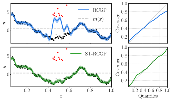
Figure 4: Simulated Temporal Data With Focussed Outliers. Left: $N=200$ points are generated from a GP with Matérn kernel ($\nu=3/2$), and contaminated with 5% outliers. RCGP uses $\gamma(x)=m(x)==\frac{1}{N}\sum_{i=1}^{N}y_{i}$ and $c=Q_{N}(0.95)$. While predictions are made on data with outliers, we fit the hyperparameters of RCGP on de-contaminated data to make it as strong a competitor as possible. In contrast, ST-RCGP uses the robust hyperparameter optimisation and selection from Section 3 to fit and predict from data with outliers. Despite this, ST-RCGP performs much better than RCGP. Right: The coverage plots measure how often the uncontaminated data falls within the predictive distribution’s $q$-th quantile.

In the remainder, we study the advantages of ST-RCGP on numerical examples. First, we investigate how ST-RCGP improves upon RCGP. Second, we explore ST-RCGP in well-specified settings without outliers. Third, we showcase its virtues on financial time series with severe outliers and its superior performance relative to competitors. Our last numerical experiment studies the robustness ST-RCGP exhibits towards spatio-temporal temperature anomalies. The code to reproduce all experiments is available at https://github.com/williamlaplante/ST-RCGP. Throughout Section 4, we evaluate experiments based on root mean squared error (RMSE) and evaluations of the negative log predictive distribution (NLPD) on the test data. To capture the tradeoff between robustness to outliers and statistical efficiency, which in our case is defined as a model’s ability to recover the standard GP in well-specified settings, we also report the expected weighted ratio (EWR), an empirical measure we expand on in Section C.1. Even when investigating temporal tasks without spatial dimensions, we keep the name ST-RCGP to clarify that inference proceeds (i) via the state-space representation of Proposition 3.1, and (ii) via hyperparameters chosen using the methods of Section 3—rather than those used for vanilla RCGPs in Altamirano et al. (2024).

Fixing vanilla RCGP

In previous sections and Figure 3, we found that vanilla RCGP is vulnerable to prior mean misspecification (Issue #1), can produce poor uncertainty estimates (Issue #2) and cannot correctly select $c$ (Issue #3). In our first experiment, we show how ST-RCGP improves on those issues. To this end, we simulate data from a GP and compare the fit produced by both algorithms in Figure 4. The plotted predictives show that RCGP is compromised by outliers due to Issue #1 and Issue #3, while the coverage plots point to unreliable uncertainty estimates induced by Issue #2. In contrast, using an adaptive centering and shrinking function allows ST-RCGP to produce reliable uncertainty estimates and predictions.

ST-RCGP in Well-Specified Settings

While robust methods offer protection from contaminated data, some can only do so at the expense of statistical efficiency. Here, we show that ST-RCGP remains statistically efficient in well-specified settings and robust to outliers when required. The setup we use is described in Section C.9, and results are reported in Table 1. While RMSE and NLPD are comparable across methods in well-specified settings, STGP suffers from a clear drop in NLPD and RMSE when outliers are introduced. In contrast, compared to other methods, the ST-RCGP maintains the lowest RMSE and NLPD in both cases. Also, its EWR is high in well-specified settings and drops in the presence of outliers to obtain robustness. The ST-RCGP thus exhibits the properties we seek out of robust methods in well-specified settings.

Table 1: EWR, RMSE, and NLPD for different methods in well-specified settings and with data containing outliers.

Outliers	Method	EWR	NLPD	RMSE
Yes	STGP	$1.0\pm 0.0$	$30\pm 2$	$0.38\pm 0.02$
	RCGP	$0.886\pm 0.001$	$6.6\pm 0.3$	$0.21\pm 0.01$
	ST-RCGP	$0.863\pm 0.002$	$5.5\pm 0.2$	$0.19\pm 0.01$
No	STGP	$1.0\pm 0.0$	$6.5\pm 0.2$	$0.19\pm 0.01$
	RCGP	$0.894\pm 0.001$	$5.6\pm 0.1$	$0.19\pm 0.01$
	ST-RCGP	$0.903\pm 0.001$	$5.7\pm 0.1$	$0.19\pm 0.01$

Robustness During Financial Crashes

On April 23rd 2013, the Associated Press’s Twitter account was hacked and posted false tweets about explosions at the White House. This led to a brief but significant market drop, including in the Dow Jones Industrial Average (DJIA), which quickly rebounded after the tweet was proven false. This data set was previously studied by Altamirano et al. (2024) and Ament et al. (2024). We plot the GP, RCGP, and ST-RCGP fits in Figure 5, as well as the robust GP via relevance pursuit (RP) fit from Ament et al. (2024). While RP behaves as desired, the plot reveals that the GP is not robust to the crash. Interestingly, the RCGP performs even worse since $\gamma$, which is chosen as the constant prior mean obtained by averaging two days of data, happens to be close to the outliers during the crash, implying that RCGP is centered around the outliers. This is another instance of Issue #1, and it is addressed by ST-RCGP. By using an adaptive centering function introduced in Section 3, ST-RCGP is centered around more reasonable values. The right-hand panel of Figure 5 also highlights that ST-RCGP leads to substantive computational gains relative to RCGP and GP due to its state-space representation from Proposition 3.1. We do not plot RP because it is implemented using a different package, and computational time is thus not comparable. But the cost of RPs is a multiple of that for GPs (Ament et al., 2024), and hence also significantly more than that of RCGPs and ST-RGCPs. It is also unclear how easily RPs could use the spatio-temporal structure to get a linear-in-time cost. For this reason, we do not explore RP beyond this experiment.

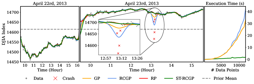
Figure 5: Comparing Estimates of DJIA Index During Twitter Flash Crash Incident. RCGP uses a prior mean of the data over the two days. We notice a dip in the posterior predictive of RCGP when the prior mean aligns with the crash event (red), whereas ST-RCGP and relevance pursuit algorithm (RP) from Ament et al. (2024) remain unaffected. In the right plot, we show computational time vs the number of data points. Note that RP has cost $K$ times the standard GP, where typically $K>1$.

Since the flash crash dataset only contains $N=810$ data points, we further explore the computational properties of ST-RCGP by considering a trading day of index futures data with $N=46,800$ data points. We then synthetically induce a crash similar to that in the previous example (see Section C.10). Naive GP implementations struggle with data of this size, and so we focus on inherently sequential methods. Table 2 summarises the results, and compares ST-RCGP against STGP, as well as several off-the-shelf inference methods for sequential GPs with Student’s $t$ errors from the BayesNewton package (Wilkinson et al., 2023) that include Markov expectation propagation (MEP), Markov variational inference (MVI), and Markov Laplace (MLa). While STGP and ST-RCGP have similar computational cost, the robustness of ST-RCGP leads to superior performance. Conversely, ST-RCGP’s performance is comparable to models using Student’s $t$ errors for this problem, but its computational cost is substantively lower. This is true despite the fact that ST-RCGP is exact, while the other robust methods in Table 2 only produce approximate inferences.

Table 2: Performance comparison on $N=46800$ data points with outliers. Below, Total (s) denotes clock time for full inference, 1-Step (ms) the estimated slope of a linear model fitted to execution time data for different data set sizes. Further, RMSE and NLPD use 1000 test points around the induced crash that are not outliers.

	Total (s)	1-Step (ms)	RMSE	NLPD
STGP	$8.0\pm 0.7$	$0.17\pm 0.01$	$0.54\pm 0.01$	$13.9\pm 0.3$
ST-RCGP	$9.4\pm 0.4$	$0.20\pm 0.02$	$0.145\pm 0.002$	$-0.62\pm 0.01$
MEP	$29.1\pm 0.5$	$0.60\pm 0.01$	$0.15\pm 0.01$	$-0.57\pm 0.03$
MVI	$28.3\pm 0.6$	$0.61\pm 0.01$	$0.15\pm 0.01$	$-0.53\pm 0.04$
MLa	$29\pm 2$	$0.62\pm 0.03$	$0.17\pm 0.01$	$-0.39\pm 0.1$

Forecasting Temperature Across the UK

Having established the performance of ST-RCGP for simpler problems, our last experiment studies its behaviour on spatio-temporal temperature data with synthetically induced outliers. In particular, we induce what are often referred to as focussed outliers, and which simulate the impact of rare natural phenomena that affect neighbouring weather stations. The data we use is collected by the Climate Research Unit (see Harris et al., 2020) and measures temperature from 16/01/2022 to 16/12/2023 at $n_{s}=571$ locations, containing $N=11,991$ data points in total. Hyperparameter optimisation is performed from 16/01/2022 to 30/09/2023, with later dates serving as test data. In October and November 2023, we perform in-sample predictions, and December 2023 is used for a one-month temperature forecast. Figure 7 and Figure 7 display the results. The two models perform similarly when there are no outliers. However, the STGP loses prediction accuracy (NLPD and RMSE) with outliers, whereas ST-RCGP maintains consistent RMSE and NLPD over time, offering more reliable predictions at comparable computational cost.

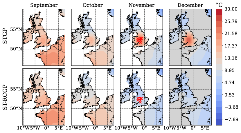
[.61] [.35] STGP ST-RCGP RMSE NLPD RMSE NLPD May 0.79 1.63 0.80 1.57 Jun 0.77 1.53 0.82 1.50 Jul 0.76 1.49 0.74 1.35 Aug 0.77 1.61 0.77 1.60 Sep 0.82 2.13 0.70 1.37 Oct 1.23 7.50 0.73 1.42 Nov 3.30 41.62 0.79 1.33 Dec 3.84 3.30 1.38 2.13

Figure 6: Temperature fit across the UK between September and December 2023. Focussed outliers appear in November and are shown as red crosses. We forecast the month of December. September is the last month included in parameter optimisation. We include September to show performance on previously seen data.

Figure 7: Performance on temperature data. Models perform inference on contaminated data, but RMSE and NLPD use outlier-free data. November introduces focussed outliers, and December is a one-step forecast.

5 Conclusion

We proposed ST-RCGPs based on an overhaul of the RCGP framework of Altamirano et al. (2024) that addressed some major drawbacks of vanilla RCGPs, further improved their computational efficiency and paved the way for using them in spatio-temporal problems. ST-RCGPs have the computational complexity of STGPs, but additionally provide robustness to outliers. Further, we empirically demonstrated that ST-RCGPs match the performance of the relevance pursuit algorithm from Ament et al. (2024) and of various robust GP methods from the BayesNewton package (Wilkinson et al., 2023) at a fraction of their computational cost and without approximation error.

Our method builds on STGPs, which remain vulnerable to scaling in the spatial dimension—an issue addressed by Hamelijnck et al. (2021) through variational approximations. The same technique could be adapted to ST-RCGPs, providing the same benefit. While this is beyond the scope of the current paper, it would constitute a natural next step for future research in this direction. An entirely different but equally relevant endeavour for future research is to explore the use of non-Gaussian likelihoods within the RCGP framework. This would extend its use beyond the standard regression setting, and allow its application to classification problems, count data, and various bounded data domains.

Acknowledgements

WL was supported by UCL’s Center for Doctoral Training in Data-Intensive Science and by the Alan Turing Institute. MA was supported by a Bloomberg Data Science PhD fellowship. FXB and JK were supported by the EPSRC grant EP/Y011805/1, and JK was addtionally supported by EP/W005859/1.

Supplementary Material

 

The Appendix is structured as follows: We first introduce notation. Then, in Appendix A, we derive the loss function used in the main paper. Next, in Appendix B, we provide the proofs of all our theoretical results. Finally, in Appendix C, we provide additional details on our numerical experiments, as well as further experiments that complement those in the main text.

Notation

Suppose we have a vector $\mathbf{v}=(v_{1},v_{2},...,v_{N})^{\top}\in\mathbb{R}^{N}$, where $v_{i}:\mathbb{R}^{d}\rightarrow\mathbb{R}$, and a matrix $\mathbf{M}\in\mathbb{R}^{N\times N}$. Then,

• $\text{diag}(\mathbf{v}):=\begin{pmatrix}v_{1}&\cdots&0&0\\ \vdots&\ddots&\vdots&\vdots\\ 0&\cdots&v_{N-1}&0\\ 0&\cdots&0&v_{N}\end{pmatrix}$ and $\text{diag}(\mathbf{M}):=(M_{11},M_{22},\dots,M_{NN})^{\top}$ where $M_{ij}:=(\mathbf{M})_{ij}$.

• $\mathbf{v}^{2}:=(v_{1}^{2},...,v_{N}^{2})^{\top}$

• $\log(\mathbf{v}):=\left(\log(v_{1}),\dots,\log(v_{N})\right)^{\top}$

• $\nabla_{y}\mathbf{v}=\left(\frac{\partial}{\partial y}v_{1},\dots,\frac{\partial}{\partial y}v_{N}\right)^{\top}$, where $\frac{\partial}{\partial y}v_{i}$ is the partial derivative of $v_{i}$ with respect to $y$.

• $\mathbf{v}\odot\mathbf{w}:=(v_{1}w_{1},...,v_{N}w_{N})^{\top}$ for $\mathbf{w}\in\mathbb{R}^{N}$.

We now remind the reader of the dimensionality of matrices and vectors crucial to the main algorithm (Proposition 3.1) of this paper:

• $\mathbf{A}_{k-1},\mathbf{\Sigma}_{k-1}\in\mathbb{R}^{n_{s}(\nu+1)\times n_{s}(\nu+1)}$ are the transition matrices from Equation 4

• $\mathbf{H}\in\mathbb{R}^{n_{s}\times n_{s}(\nu+1)}$ is the measurement matrix from Equation 4

• $\mathbf{y}_{k},\;\mathbf{w}_{k},\;\hat{\mathbf{f}}_{k}^{\text{GB}}\in\mathbb{R}^{n_{s}}$ are the observations, weights and filtering predictives from Proposition 3.1.

• $\mathbf{P}_{k|k}^{\text{GB}}\in\mathbb{R}^{n_{s}(\nu+1)\times n_{s}(\nu+1)}$ is the covariance matrix from Proposition 3.1

• $\mathbf{m}_{k|k}^{\text{GB}}\in\mathbb{R}^{n_{s}(\nu+1)}$ is the mean from Proposition 3.1

• $\mathbf{K}_{k}^{\text{GB}}\in\mathbb{R}^{n_{s}(\nu+1)\times n_{s}}$ is the Kalman gain matrix from Proposition 3.1

• $\mathbf{J}_{\mathbf{w}_{k}}\in\mathbb{R}^{n_{s}\times n_{s}}$ is the weight-based matrix from Proposition 3.1.

Finally, when we use $p(\cdot)=\mathcal{N}(\cdot\;;\mu,\Sigma)$, we are referring to the density of the normal distribution with mean $\mu$ and covariance $\Sigma$, and when we use $\mathcal{N}(\mu,\Sigma)$, we are referring to the distribution.

Appendix A Score-Matching & Loss Function

This section provides the derivation of the loss function used in the main paper based on the weighted Fisher divergence.

We define the weighted Fisher divergence at a fixed time $t_{k}$. Let $f_{k}(.)=f(.,t_{k})$ the spatial model at time $t_{k}$. Let $p_{k}(y|s)=p(y|s,t_{k})$ be the density of the true data-generating process at time $t_{k}$, and $p_{f_{k}}(y|s)=p(y|f_{k}(s))$ be the density of our model at time $t_{k}$.

The weighted Fisher divergence for regression between the model and data-generating process at time $t_{k}$ depends on the corresponding scores $s_{f_{k}}(y|s)=\nabla_{y}\log p_{f_{k}}(y|s)$ and $s_{k}(y|s)=\nabla_{y}\log p_{k}(y|s)$ and is given by Barp et al. [2019], Xu et al. [2022], Altamirano et al. [2024]:

$$\mathcal{D}_{k} :=\mathbb{E}_{S\sim p_{k,s}}\left[\mathbb{E}_{Y\sim p_{k}(.|S)}\left[\left\|w_{k}(S,Y)\left(s_{k}(Y|S)-s_{f_{k}}(Y|S)\right)\right\|_{2}^{2}\right]\right]$$

$$\overset{+C}{=}\mathbb{E}_{S\sim p_{k,s}}\left[\mathbb{E}_{Y\sim p_{k}(.|S)}\left[\left\|w_{k}(S,Y)s_{f_{k}}(Y|S)\right\|_{2}^{2}+2\nabla_{y}\cdot\left(w_{k}(S,Y)^{2}s_{f_{k}}(Y|S)\right)\right]\right],$$

where $p_{k,s}=p(s|t_{k})$ is the marginal, $w_{k}(s,y)=w((s,t_{k}),y)$, and the equality—which crucially does not depend on $s_{k}$ anymore—holds up to an additive constant $C$ not depending on $f_{k}$.

Now, consider a dataset such that $\mathbf{x}_{k}=({\mathbf{x}}_{k,1},...,{\mathbf{x}}_{k,n_{s}})^{\top}$, for $\mathbf{x}_{k,j}=(\mathbf{s}_{j},t_{k})\in\mathcal{X}=\mathcal{S}\times\mathcal{T}$, ${\mathbf{y}}_{k}=(y_{k,1},...,y_{k,n_{s}})^{\top}$, and let ${\mathbf{f}}_{k}:={\mathbf{f}}({\mathbf{x}}_{k})=(f({\mathbf{x}}_{k,1}),...,f({\mathbf{x}}_{k,n_{s}}))^{\top}$. Moreover, let $\mathbf{z}_{k}$ be related to ${\mathbf{f}}_{k}$ as ${\mathbf{f}}_{k}:=\mathbf{H}\mathbf{z}_{k}$. The empirical loss we obtain for filtering is then

$$\mathcal{L}(\mathbf{x}_{k},\mathbf{y}_{k},\mathbf{z}_{k})=\frac{1}{n_{s}}\sum_{j=1}^{n_{s}}\|w_{k,j}s_{f,k,j}\|_{2}^{2}+2\nabla_{y}\cdot\left((w_{k,j})^{2}s_{f,k,j}\right),$$ (10)

where $w_{k,j}=w(\mathbf{x}_{k,j},y_{k,j})$, and $s_{f,k,j}=s_{f_{k}}(y_{k,j})$.

Appendix B Proofs of Theoretical Results

B.1 Proof of Proposition 3.1

In the following, we derive the Generalised Bayes filtering posterior distribution when the loss function is quadratic. We then show that the weighted score matching loss with a Gaussian model yields a quadratic loss. Finally, we provide the derivation of the GB predictive.

Let us assume a quadratic loss in $\mathbf{z}_{k}$ or equivalently in $\mathbf{f}_{k}:=\mathbf{H}\mathbf{z}_{k}$ of the form:

$$\mathcal{L}(\mathbf{z}_{k},\mathbf{y}_{k},\mathbf{x}_{k})=\frac{1}{2n_{s}}\left(\mathbf{f}_{k}^{\top}\mathbf{R}^{-1}_{k}\mathbf{f}_{k}-\mathbf{f}_{k}^{\top}\mathbf{v}_{k}+C_{k}\right),$$

where $R_{k}\in{\mathbb{R}}^{n_{s}\times n_{s}}$ is an invertible matrix, $v_{k}\in{\mathbb{R}}^{n_{s}}$, and $C_{k}\in{\mathbb{R}}$. The GB filtering update equations are then

$$\begin{split}p_{\mathcal{L}}(\mathbf{z}_{k}|\mathbf{y}_{1:k})&\propto p(\mathbf{z}_{k}|\mathbf{y}_{1:k-1})\exp(-n_{s}\mathcal{L}(\mathbf{y}_{k};\mathbf{z}_{k}))\\ &\propto\exp\left(-\frac{1}{2}(\mathbf{z}_{k}-\mathbf{m}_{k|k-1})^{\top}\mathbf{P}_{k|k-1}^{-1}(\mathbf{z}_{k}-\mathbf{m}_{k|k-1})\right)\exp\left(-\frac{1}{2}\left(\mathbf{f}_{k}^{\top}\mathbf{R}_{k}^{-1}\mathbf{f}_{k}-2\mathbf{f}_{k}^{\top}\mathbf{v}_{k}\right)\right)\\ &\propto\exp\left(-\frac{1}{2}\left(\mathbf{z}_{k}^{\top}(\mathbf{P}_{k|k-1}^{-1}+\mathbf{H}^{\top}\mathbf{R}_{k}^{-1}\mathbf{H})\mathbf{z}_{k}-2\mathbf{z}_{k}^{\top}(\mathbf{P}_{k|k-1}^{-1}\mathbf{m}_{k|k-1}+\mathbf{H}^{\top}\mathbf{v}_{k})\right)\right),\end{split}$$ (11)

which implies that the mean $\mathbf{m}_{k|k}^{\text{GB}}$ and covariance $\mathbf{P}_{k|k}^{\text{GB}}$ of the GB posterior $p_{\mathcal{L}}$ are:

$$\begin{split}&\mathbf{P}_{k|k}^{\text{GB}}=\left(\mathbf{P}_{k|k-1}^{-1}+\mathbf{H}^{\top}\mathbf{R}_{k}^{-1}\mathbf{H}\right)^{-1}\\ &\mathbf{m}_{k|k}^{\text{GB}}=\mathbf{P}_{k|k}^{\text{GB}}\left(\mathbf{P}_{k|k-1}^{-1}\mathbf{m}_{k|k-1}+\mathbf{H}^{\top}\mathbf{v}_{k}\right).\end{split}$$ (12)

As with the typical Kalman filter, those equations can be written in the form

$$\begin{split}&\mathbf{P}_{k|k}^{\text{GB}}=\left(\mathbf{P}_{k|k-1}^{-1}+\mathbf{H}^{\top}\mathbf{R}_{k}^{-1}\mathbf{H}\right)^{-1}\\ &\mathbf{K}_{k}^{\text{GB}}=\mathbf{P}_{k|k}^{\text{GB}}\mathbf{H}^{\top}\mathbf{R}_{k}^{-1}\\ &\mathbf{m}_{k|k}^{\text{GB}}=\mathbf{m}_{k|k-1}+\mathbf{K}_{k}^{\text{GB}}(\mathbf{R}_{k}\mathbf{v}_{k}-\mathbf{H}\mathbf{m}_{k|k-1}),\end{split}$$ (13)

where $\mathbf{K}_{k}^{\text{GB}}$ is the Kalman gain matrix. The typical Kalman filter equations—those used for STGPs—are recovered when $\mathbf{v}_{k}:=\mathbf{R}^{-1}_{k}\mathbf{y}_{k}$ and $\mathbf{R}_{k}^{-1}:=\sigma^{-2}\mathbf{I}_{n_{s}}$.

Weighted score matching and Gaussian likelihood.

We now show that the loss function defined in Appendix A and Gaussian likelihood lead to a quadratic loss in $\mathbf{f}_{k}$. We have a Gaussian likelihood, which gives a score function of the form:

$$p(\mathbf{y}_{k}|\mathbf{z}_{k},{\mathbf{x}}_{k})\propto\exp\left(-\frac{1}{2}(\mathbf{y}_{k}-\mathbf{f}_{k})^{\top}\sigma^{-2}\mathbf{I}_{n_{s}}(\mathbf{y}_{k}-\mathbf{f}_{k})\right)\implies\mathbf{s}_{f,k}=\nabla_{y}\log p({\mathbf{y}}_{k}|f_{k})=(\mathbf{f}_{k}-\mathbf{y}_{k})^{\top}\sigma^{-2}\mathbf{I}_{n_{s}},$$ (14)

where $\mathbf{f}_{k}:=\mathbf{H}\mathbf{z}_{k}$, $\mathbf{z}_{k}=(z_{k,1},...,z_{k,n_{s}})^{\top}$, $\mathbf{y}_{k}=(y_{k,1},...,y_{k,n_{s}})^{\top}$ and $\mathbf{s}_{f,k}=(s_{f,k,1},...,s_{f,k,n_{s}})^{\top}$. Then, the loss is given by

$$\mathcal{L}(\mathbf{y}_{k},\mathbf{z}_{k})= \frac{1}{n_{s}}\sum_{j=1}^{n_{s}}\left(w_{k,j}s_{f,k,j}\right)^{2}+2\nabla_{y}\left(w_{k,j}^{2}s_{f,k,j}\right)$$

$$= \frac{1}{n_{s}}\sum_{j=1}^{n_{s}}\left(w_{k,j}\frac{(f_{k,j}-y_{k,j})}{\sigma^{2}}\right)^{2}+2\nabla_{y}\left(w_{k,j}^{2}\frac{(f_{k,j}-y_{k,j})}{\sigma^{2}}\right)$$

$$= \frac{1}{n_{s}}\sum_{j=1}^{n_{s}}\frac{1}{\sigma^{4}}w_{k,j}^{2}f_{k,j}^{2}-\frac{2}{\sigma^{4}}f_{k,j}y_{k,j}w_{k,j}^{2}+\frac{1}{\sigma^{4}}w_{k,j}^{2}y_{k,j}^{2}+\frac{2}{\sigma^{2}}\nabla_{y}(w_{k,j}^{2}f_{k,j})-\frac{2}{\sigma^{2}}\nabla_{y}(w_{k,j}^{2}y_{k,j})$$

Now let us group all the elements that do not depend on $f$ and call it $C(y_{k,j})$

$$\mathcal{L}(\mathbf{y}_{k},\mathbf{z}_{k})= \frac{1}{n_{s}}\sum_{j=1}^{n_{s}}\frac{1}{\sigma^{4}}w_{k,j}^{2}f_{k,j}^{2}-\frac{2}{\sigma^{4}}f_{k,j}y_{k,j}w_{k,j}^{2}+\frac{2}{\sigma^{2}}\nabla_{y}(w_{k,j}^{2}f_{k,j})+C(y_{k,j})$$

$$= \frac{1}{n_{s}}\sum_{j=1}^{n_{s}}\frac{1}{\sigma^{4}}w_{k,j}^{2}f_{k,j}^{2}-\frac{2}{\sigma^{4}}f_{k,j}y_{k,j}w_{k,j}^{2}+\frac{4}{\sigma^{2}}w_{k,j}f_{k,j}\nabla_{y}w_{k,j}+C(y_{k,j})$$

$$= \frac{1}{n_{s}}\sum_{j=1}^{n_{s}}\frac{1}{\sigma^{4}}w_{k,j}^{2}f_{k,j}^{2}-\frac{2}{\sigma^{4}}w_{k,j}^{2}\left(y_{k,j}-2\sigma^{2}(w_{k,j})^{-1}\nabla_{y}w_{k,j}\right)f_{k,j}+C(y_{k,j})$$

Next, we rewrite the loss in terms of vectors and matrices as follows:

$$\mathcal{L}(\mathbf{y}_{k},\mathbf{z}_{k})= \frac{1}{2n_{s}}\left(\frac{2}{\sigma^{4}}\mathbf{f}_{k}^{\top}\text{diag}(\mathbf{w}_{k}^{2})\mathbf{f}_{k}-\frac{4}{\sigma^{4}}\mathbf{f}_{k}^{\top}\left(\text{diag}(\mathbf{w}_{k}^{2})\mathbf{y}_{k}-2\sigma^{2}\text{diag}(\mathbf{w}_{k})\nabla_{y}\mathbf{w}_{k}+C({\mathbf{y}}_{k})\right)\right),$$

where $C({\mathbf{y}}_{k})=\sum_{j=1}^{n_{s}}C(y_{k,j})$, $\text{diag}(\mathbf{w}_{k}^{2})\in\mathbb{R}^{n_{s}\times n_{s}}$ is the diagonal matrix of the vector $\mathbf{w}_{k}^{2}=\mathbf{w}_{k}\odot\mathbf{w}_{k}$ for $\odot$ the element-wise multiplication operator, and $\nabla_{y}\mathbf{w}_{k}=(\nabla_{y}w_{k,1},...,\nabla_{y}w_{k,n_{s}})^{\top}$. This leads to

$$\begin{split}&\mathbf{R}^{-1}(\mathbf{y}_{k};\mathbf{w}_{k}):=\frac{2}{\sigma^{4}}\text{diag}(\mathbf{w}_{k}^{2})\\ &\mathbf{v}_{k}(\mathbf{y}_{k};\mathbf{w}_{k}):=\frac{2}{\sigma^{4}}\left(\text{diag}(\mathbf{w}_{k}^{2})\mathbf{y}_{k}-2\sigma^{2}\text{diag}(\mathbf{w}_{k})\nabla_{y}\mathbf{w}_{k}\right).\end{split}$$ (15)

GP predictive

The GB predictive can be written as:

$$p_{\mathcal{L}}({\mathbf{y}}_{k}|{\mathbf{y}}_{1:k-1})=\int p({\mathbf{y}}_{k}|\mathbf{z}_{k})p_{\mathcal{L}}(\mathbf{z}_{k}|y_{1:k-1})d\mathbf{z}_{k}$$

where $p({\mathbf{y}}_{k}|\mathbf{z}_{k})=\mathcal{N}(\mathbf{y}_{k};\mathbf{H}\mathbf{z}_{k},\sigma^{2}\mathbf{I}_{n_{s}})$ is the likelihood and $p_{\mathcal{L}}(\mathbf{z}_{k}|\mathbf{y}_{1:k-1})=\mathcal{N}(\mathbf{z}_{k};\mathbf{m}_{k|k-1},\mathbf{P}_{k|k-1})$ is the predict step defined in Proposition 3.1. Since both densities are Gaussian, this integral is known and the solution is also a Gaussian of the form:

$$p_{\mathcal{L}}({\mathbf{y}}_{k}|{\mathbf{y}}_{1:k-1}) =\int\mathcal{N}(\mathbf{y}_{k};\mathbf{H}\mathbf{z}_{k},\sigma^{2}\mathbf{I}_{n_{s}})\mathcal{N}(\mathbf{z}_{k};\mathbf{m}_{k|k-1},\mathbf{P}_{k|k-1})d\mathbf{z}_{k}$$

$$=\mathcal{N}(\mathbf{y}_{k};\mathbf{H}\mathbf{m}_{k|k-1},\mathbf{H}\mathbf{P}_{k|k-1}\mathbf{H}^{\top}+\sigma^{2}\mathbf{I}_{n_{s}})$$

B.2 Proof of Proposition 3.2

To prove the robustness of ST-RCGP, we rely on the fact that ST-RCGP and RCGP share the same distribution for spatio-temporal data; therefore, we could use the following result from Altamirano et al. [2024] adapted to the spatio-temporal setting:

Proposition B.1 (Altamirano et al. [2024]).

Suppose ${\mathbf{f}}\sim\mathcal{GP}(m,k)$, $(\epsilon_{1},...,\epsilon_{N})^{\top}\sim\mathcal{N}(0,\mathbf{I}_{N}\sigma^{2})$, and let $C_{k}\in{\mathbb{R}};k=1,2$ be constants independent of $y_{m,j}^{c}$. Then, for RCGP regression with $\sup_{{\mathbf{x}}\in\mathcal{X},y\in\mathcal{Y}}w({\mathbf{x}},y)<\infty$ has the PIF

$$\operatorname{PIF}(y_{m,j}^{c},D)\leq C_{1}(w({\mathbf{x}}_{m,j},y^{c}_{m,j})^{2}y^{c}_{m,j})^{2}+C_{2}.$$ (16)

Thus, if $\forall{\mathbf{x}}\in\mathcal{X}$, $\sup_{y\in\mathcal{Y}}\left|y\cdot w({\mathbf{x}},y)^{2}\right|<\infty$ , RCGP is robust since $\sup_{y^{c}_{m,j}\in\mathcal{Y}}|\operatorname{PIF}_{\operatorname{RCGP}}(y^{c}_{m,j},D)|<\infty$.

Hence, it suffices to verify that the proposed weight function satisfies the necessary conditions for robustness presented in Proposition B.1.

The weight function and the hyperparameter recommended are:

$$w_{\text{IMQ}}(\mathbf{x},y)=\beta\left(1+\frac{(y-\gamma(\mathbf{x}))^{2}}{c(\mathbf{x})^{2}}\right)^{-\frac{1}{2}},$$ (17)

with $\beta=\frac{\sigma^{2}}{2}$, $\gamma(\mathbf{x}):=\mathbb{E}_{p_{\mathcal{L}}}[y]$, and $c^{2}(\mathbf{x}):=\mathbb{E}_{p_{\mathcal{L}}}[(y-\gamma(\mathbf{x}))^{2}]$.

It is straightforward to verify that $w_{\text{IMQ}}(\mathbf{x},y)\leq\beta$ for all $\mathbf{x}\in\mathcal{X}$ and $y\in\mathcal{Y}$. Since $\beta=\frac{\sigma^{2}}{2}<+\infty$, it follows that $\sup_{\mathbf{x}\in\mathcal{X},y\in\mathcal{Y}}w(\mathbf{x},y)<+\infty$. Thus, with the recommended hyperparameters, $w$ satisfies the first condition.

Now, we need to check the second condition, which is that $\forall{\mathbf{x}}\in\mathcal{X},\,\sup_{y\in\mathcal{Y}}\left|y\right|\cdot w(\mathbf{x},y)^{2}<+\infty$. To show this, let us consider an arbitrary ${\mathbf{x}}\in\mathcal{X}$ and two cases for $y$:

Case 1: $|y|\leq|\gamma({\mathbf{x}})|+|c({\mathbf{x}})|$

Since $w_{\text{IMQ}}(\mathbf{x},y)\leq\beta$ for all $\mathbf{x}\in\mathcal{X}$ and $y\in\mathcal{Y}$, it follows:

$$\left|y\right|\cdot w(\mathbf{x},y)^{2} \leq|y|\beta^{2}\leq\beta^{2}(|\gamma({\mathbf{x}})|+|c({\mathbf{x}})|)$$

Which implies that, as long as $|\gamma({\mathbf{x}})|<\infty$ and $|c({\mathbf{x}})|<\infty$ we have that:

$$\sup_{\begin{subarray}{c}y\in\mathcal{Y}\\ s.t.|y|\leq|\gamma({\mathbf{x}})|+|c({\mathbf{x}})|\}\end{subarray}}\left|y\right|\cdot w(\mathbf{x},y)^{2}<\infty$$

Case 2: $|y|>|\gamma({\mathbf{x}})|+|c({\mathbf{x}})|$

$$\left|y\right|\cdot w(\mathbf{x},y)^{2} \leq|y|\beta^{2}\frac{1}{1+\frac{(y-\gamma(\mathbf{x}))^{2}}{c(\mathbf{x})^{2}}}\leq|y|\beta^{2}\frac{1}{\frac{(y-\gamma(\mathbf{x}))^{2}}{c(\mathbf{x})^{2}}}=|y|\beta^{2}\frac{c(\mathbf{x})^{2}}{(y-\gamma(\mathbf{x}))^{2}}=\beta^{2}\frac{c(\mathbf{x})^{2}}{|y|\left(1-\frac{\gamma(\mathbf{x})}{y}\right)^{2}}$$

Now, we observe that this function is decreasing for $|y|>|\gamma({\mathbf{x}})|+|c({\mathbf{x}})|$, and particularly:

$$\lim_{|y|\to+\infty}\beta^{2}\frac{c(\mathbf{x})^{2}}{|y|\left(1-\frac{\gamma(\mathbf{x})}{y}\right)^{2}}=0,$$

since $|y|>|\gamma({\mathbf{x}})|$. Therefore, attains its maximum at $|y|=|\gamma({\mathbf{x}})|+|c({\mathbf{x}})|$, which leads to the following bound:

$$\left|y\right|\cdot w(\mathbf{x},y)^{2} \leq\beta^{2}\frac{c(\mathbf{x})^{2}}{|y|\left(1-\frac{\gamma(\mathbf{x})}{y}\right)^{2}}\leq\beta^{2}(|\gamma({\mathbf{x}})|+|c({\mathbf{x}})|).$$

Which implies that, as long as $|\gamma({\mathbf{x}})|<\infty$ and $|c({\mathbf{x}})|<\infty$ we have that:

$$\sup_{\begin{subarray}{c}y\in\mathcal{Y}\\ s.t.|y|>|\gamma({\mathbf{x}})|+|c({\mathbf{x}})|\}\end{subarray}}\left|y\right|\cdot w(\mathbf{x},y)^{2}<\infty.$$

Finally, let us check that $|\gamma({\mathbf{x}})|<\infty$ and $|c({\mathbf{x}})|<\infty$. Since $\gamma({\mathbf{x}})=\mathbb{E}_{p_{\mathcal{L}}}[y]$ and $c^{2}(\mathbf{x}):=\mathbb{E}_{p_{\mathcal{L}}}[(y-\gamma(\mathbf{x}))^{2}]$ are the mean and the variance of $p_{\mathcal{L}}(y|{\mathbf{x}})$ respectively, and $p_{\mathcal{L}}(y|{\mathbf{x}})$ is a Gaussian, we know that the $|\gamma({\mathbf{x}})|<\infty$ and $|c({\mathbf{x}})|<\infty$.

Putting it all together, we have that:

$$\forall x\in\mathcal{X},\,\sup_{y\in\mathcal{Y}}\left|y\right|\cdot w(\mathbf{x},y)^{2}<\infty.$$

Appendix C Additional Numerical Experiments

C.1 Performance Metrics

Let $p_{0}(\cdot|\mathbf{x})$ be the density of the true data-generating process on the spatio-temporal grid $\mathbf{X}=(\mathbf{x}_{1},\dots,\mathbf{x}_{k})^{\top}\in\mathcal{X}^{n_{t}}$. The first performance metric we use is the root mean squared error (RMSE):

$$\mathrm{RMSE}(\mathbf{X},\hat{y}):=\sqrt{\mathbb{E}_{Y\sim p_{0}(\cdot|\mathbf{X})}\left[(Y-\hat{y})^{2}\right]}\approx\sqrt{\frac{1}{n_{t}n_{s}}\sum_{k=1}^{n_{t}}\sum_{j=1}^{n_{s}}\left(y_{k,j}-\hat{y}_{k,j}\right)^{2}},$$

where $N=n_{t}n_{s}$ is the number of data points, $y_{i}$ is the data, and $\hat{y}_{i}$ is the model’s prediction. The second performance metric we use is the negative log predictive distribution (NLPD):

$$\mathrm{NLPD}(\mathbf{X},\hat{y}):=\mathbb{E}_{Y\sim p_{0}(\cdot|\mathbf{X})}\left[-\log p_{\phi}\left(Y|\hat{y}\right)\right]\approx-\frac{1}{N}\sum_{i=1}^{N}\log p_{\phi}(y_{i}\mid\hat{y}_{i},\hat{\sigma}^{2}),$$

where $\hat{\sigma}^{2}$ is the model’s variance, and $p_{\phi}$ is the standard normal density. Finally, for the methods with weights such as RCGP and ST-RCGP, we introduce the expected weight ratio (EWR):

$$\text{EWR}(\mathbf{X}):=\mathbb{E}_{Y\sim p_{0}(\cdot|\mathbf{X})}\left[\frac{w(\mathbf{x},Y)}{w_{\text{STGP}}(\mathbf{x},Y)}\right]\approx\frac{1}{n_{t}n_{s}}\sum_{k=1}^{n_{t}}\sum_{j=1}^{n_{s}}\left(1+\frac{(y_{k,j}-\gamma(\mathbf{x}_{k,j}))^{2}}{c(\mathbf{x}_{k,j})^{2}}\right)^{-\frac{1}{2}},$$

where $w_{\text{STGP}}:=\sigma/\sqrt{2}$ is the constant weight for the standard spatio-temporal GP. Note that by construction, $\textrm{EWR}\leq 1$. In particular, if $w_{k}=w_{\text{STGP}}$ for all $k=1,...,n_{t}$, then $\text{EWR}=1$ and we recover the STGP posterior exactly. However, since the STGP is not robust to outliers, the closer EWR is to one, the less robust our posterior is to outliers, and vice-versa. This metric thus conveys a tradeoff between statistical efficiency—a model’s ability to recover the STGP in well-specified settings—and robustness to outliers. In well-specified settings, we then want EWR to be larger and closer to one. When there are outliers, we wish the opposite so that we benefit from robustness.

C.2 Implementation Details

All experiments are run on the CPU of a 2020 13-inch Macbook Pro with M1 chip and 8GB of memory.

Definition of Matrices $\mathbf{A}_{k-1}$ and $\mathbf{\Sigma}_{k-1}$

In the following, we provide a few examples of the SDE matrices needed to compute $\mathbf{A}_{k-1}$ and $\mathbf{\Sigma}_{k-1}$, and explain how they are obtained in practice. We define $\mathbf{A}_{k-1}:=\exp(\mathbf{F}\Delta t_{k})$ and

$$\begin{split}&\mathbf{\Sigma}_{k-1}:=\int_{0}^{\Delta t_{k}}e^{\mathbf{F}(\Delta t_{k}-\tau)}\mathbf{L}\mathbf{Q}_{c}\mathbf{L}^{\top}e^{{\mathbf{F}(\Delta t_{k}-\tau)}^{\top}}d\tau,\end{split}$$ (18)

where $\mathbf{F}=\mathbf{I}_{n_{s}}\otimes\mathbf{F}_{t}\in\mathbb{R}^{n_{s}(\nu+1)\times n_{s}(\nu+1)}$, $\mathbf{L}=\mathbf{I}_{n_{s}}\otimes\mathbf{L}_{t}\in\mathbb{R}^{n_{s}(\nu+1)\times n_{s}}$, and $\mathbf{Q}_{c}=\mathbf{K}_{s}\otimes\mathbf{Q}_{c,t}\in\mathbb{R}^{n_{s}\times n_{s}(\nu+1)}$ for $(\mathbf{K}_{s})_{ij}=\kappa_{s}(\mathbf{s}_{i},\mathbf{s}_{j})$. The notation $\otimes$ refers to the Kronecker product of matrices, and the term $\exp(\mathbf{F}\Delta t_{k})$ corresponds to the matrix exponential. From Equation 18, we see that the matrices $\mathbf{A}_{k-1}$ and $\mathbf{\Sigma}_{k-1}$for $k=1,...,n_{t}$ are derived from $\mathbf{F}_{t}$, $\mathbf{L}_{t}$ and $\mathbf{Q}_{c,t}$ in the SDE formulation.

SDE Matrices for Common Kernels

We provide in Table 3 common kernels and their SDE matrices. That is, for each kernel we select, we specify the matrix form of $\mathbf{F}_{t},\mathbf{L}_{t}$, along with $\mathbf{Q}_{c,t}$. We later explain how these can be used to compute $\mathbf{A}_{k-1}$ and $\mathbf{Q}_{k-1}$. The parameters in Table 3 are the lengthscale $\ell$, the amplitude $\sigma_{\kappa}$, and the period length $\omega_{0}$; the inputs of the kernels are $t,t^{\prime}\in\mathbb{R}$ and $\tau:=t-t^{\prime}$; the functions used are the Gamma function $\Gamma$ and $K_{\nu}$ is the modified Bessel function of the second kind.

Table 3: Table of kernels and their corresponding SDE matrices

Kernel	Formula	Parameters	$\mathbf{F}_{t}$	$\mathbf{L}_{t}$	$\mathbf{Q}_{c,t}$
Wiener Process	$\kappa_{\text{WP}}(t,t^{\prime}):=\sigma_{\kappa}^{2}\min(t,t^{\prime})$	$\sigma_{\kappa}$	0	1	$\sigma_{\kappa}^{2}$
Exponential	$\kappa_{\text{exp}}(\tau):=\sigma_{\kappa}^{2}\exp(-\frac{\tau}{\ell})$	$\sigma_{\kappa},\ell$	$-1/\ell$	1	$2\sigma_{\kappa}^{2}/\ell$
Matérn $\nu=1/2$ kernel	$\kappa_{\text{Mat.}}(\tau):=\sigma_{\kappa}^{2}\frac{2^{1-\nu}}{\Gamma(\nu)}\left(\frac{\sqrt{2\nu}\tau}{\ell}\right)^{\nu}K_{\nu}\left(\frac{\sqrt{2\nu}\tau}{\ell}\right)$	$\sigma_{\kappa},\ell$; $\lambda:=\sqrt{3}/\ell$	$\begin{pmatrix}0&1\\ -\lambda^{2}&-2\lambda\end{pmatrix}$	$\begin{pmatrix}0\\ 1\end{pmatrix}$	$4\lambda^{3}\sigma_{\kappa}^{2}$
Matérn $\nu=3/2$ kernel	(same as above)	$\sigma_{\kappa},\ell$; $\lambda:=\sqrt{5}/\ell$	$\begin{pmatrix}0&1&0\\ 0&0&1\\ -\lambda^{3}&-3\lambda^{2}&-3\lambda\end{pmatrix}$	$\begin{pmatrix}0\\ 0\\ 1\end{pmatrix}$	$16\sigma_{\kappa}^{2}\lambda^{5}/3$
Periodic	$\kappa_{\text{periodic}}(\tau):=\sigma_{\kappa}^{2}\exp\left(-\frac{2\sin^{2}(\omega_{0}\tau/2)}{\ell^{2}}\right)$	$\sigma_{\kappa},\ell,\omega_{0}$	$\sum_{j=1}^{n}\begin{pmatrix}0&-\omega_{0}j\\ \omega_{0}j&0\end{pmatrix}$	$n\mathbf{I}_{2}$	$\mathbf{0}$

The matrix $\mathbf{A}_{k-1}$ can be straightforwardly computed in most programming languages that offer linear algebra computations.

The covariance matrix $\mathbf{\Sigma}_{t,k-1}$ is rarely computed directly; instead, it is obtained by Matrix Fraction Decomposition (MFD) (see Chapter 6 of Särkkä and Solin [2019] for an overview of the method). Provided that the matrix $\mathbf{F}_{t}$ is Hurwitz, that is, all its eigenvalues have strictly negative real parts, the procedure to compute $\mathbf{\Sigma}_{t,k-1}$ can be further simplified Särkkä and Solin [2019] (i.e., no need for MFD) to

$$\begin{split}&\mathbf{\Sigma}_{t,0}=\mathbf{\Sigma}_{t,\infty}\\ &\mathbf{\Sigma}_{t,k-1}=\mathbf{\Sigma}_{t,\infty}-\mathbf{A}_{t,k-1}\mathbf{\Sigma}_{t,\infty}\mathbf{A}_{t,k-1}^{\top},\end{split}$$

where the initial covariance $\mathbf{\Sigma}_{t,0}$ can be found via the steady-state solution by solving for $\mathbf{\Sigma}_{t,\infty}$ in the following continuous Lyapunov equation [Särkkä and Solin, 2019, Hartikainen and Särkkä, 2010]

$$\mathbf{F}_{t}\mathbf{\Sigma}_{t,\infty}+\mathbf{\Sigma}_{t,\infty}\mathbf{F}_{t}^{\top}+\mathbf{L}_{t}\mathbf{Q}_{c,t}\mathbf{L}_{t}^{\top}=\mathbf{0}.$$

Note that we provide the full implementation for the ST-RCGP and the STGP in our code.

C.3 Robust Hyperparameter Optimisation

Issue With RCGP

Although the RCGP method is robust in inference, it still has well-known problems with hyperparameter optimisation when there are outliers. The method used is outlined in Altamirano et al. [2024], which corresponds to the leave-one-out cross-validation (LOO-CV). The optimisation objective is posed as follows:

$$\hat{\sigma}^{2},\hat{\theta}:=\arg\max_{\sigma^{2},\theta}\left\{\sum_{i=1}^{n}\log p^{w}(y_{i}|\mathbf{x},\mathbf{y}_{-i},\theta,\sigma^{2})\right\},$$

where $\mathbf{y}_{-i}=(y_{1},\dots,y_{i-1},y_{i+1},\dots,y_{n})$. Moreover, the pseudo marginal likelihood is given by $p^{w}(y_{i}|\mathbf{x},\mathbf{y}_{-i},\theta,\sigma^{2})=\mathcal{N}(\mu_{i}^{R},\sigma_{i}^{R}+\sigma^{2})$, where

$$\begin{split}\mu_{i}^{R}&:=z_{i}+\mathbf{m}_{i}-\left[\left(\mathbf{K}+\sigma^{2}\mathbf{J}_{\mathbf{w}}\right)^{-1}(\mathbf{y}-\mathbf{m}_{\mathbf{w}})\right]_{i}\;\left[\left(\mathbf{K}+\sigma^{2}\mathbf{J}_{\mathbf{w}}\right)^{-1}\right]_{ii}^{-1}\\ \sigma_{i}^{R}&:=\left[\left(\mathbf{K}+\sigma^{2}\mathbf{J}_{\mathbf{w}}\right)^{-1}\right]_{ii}^{-1}-\frac{\sigma^{4}}{2}w(x_{i},y_{i})^{-2},\end{split}$$

where the notation follows that of Equation 8.

In Figure 8, we simulate data $y$ with outliers to highlight the issue. We generate 80 data points from a GP with Squared Exponential kernel of amplitude $\sigma_{\kappa}=0.2$, lengthscale $\ell=1$, and variance $\sigma^{2}=0.01$ in normally distributed data. We position four outliers around the $y=2$ mark. To fit the data, we follow the suggested approach from Altamirano et al. [2024] and use a constant mean function equal to the arithmetic average of the data. In Figure 8, we show the results. Clearly, the RCGP fitting the data with outliers fails to produce adequate hyperparameters, whereas the fit on outlier-free data does well.

Figure 8: RCGP Parameter Optimisation With and Without Outliers. The fit with outliers yields a kernel lengthscale of 0.19, a kernel amplitude of 0.99, and variance of 0.026. The fit without outliers yields a kernel lengthscale of 1.46, a kernel amplitude of 36.9, and variance of 0.0066.

Issue with STGPs Hyperparameter Optimisation

the optimisation objective for STGPs is typically

$$\varphi(\bm{\theta}):=-\sum_{k=1}^{n_{t}}\log p(\mathbf{y}_{k}|\mathbf{y}_{1:k-1},\bm{\theta})=-\frac{1}{2}\sum_{k=1}^{n_{t}}\log|2\pi\mathbf{S}_{k}(\bm{\theta})|+\bm{\varepsilon}_{k}^{\top}(\bm{\theta})\mathbf{S}^{-1}_{k}(\bm{\theta})\bm{\varepsilon}_{k}(\bm{\theta}),$$

where $\mathbf{S}_{k}(\bm{\theta}):=\sigma^{2}\mathbf{I}_{n_{s}}+\mathbf{H}\mathbf{P}_{k|k-1}(\bm{\theta})\mathbf{H}^{\top}$ and $\bm{\varepsilon}_{k}:=\mathbf{y}_{k}-\hat{\mathbf{f}}_{k}(\bm{\theta})$.

However, with outliers, this objective does not perform well since reasonable estimates of the latent function will have large $\bm{\varepsilon}_{k}$ and thus small $p(\mathbf{y}_{k}|\mathbf{y}_{1:k-1},\bm{\theta})$—effectively fitting the outliers. This makes it so $\varphi$ may have a global minimum $\bm{\theta}^{\star}$ vastly different from the one in well-specified settings, in which case we could not recover the true latent function. We show in Figure 9 what happens when we fit STGP with a $\varphi$ objective. On the left side of the plot, we fit and make predictions with contaminated data. On the right side of the plot, we fit de-contaminated data and make predictions on data with outliers. Both approaches yield undesired results, but most importantly, they are vastly different—a result that stems from introducing outliers in the data used for hyperparameter optimisation. Overall, Figure 9 shows that $\varphi$ is strongly affected by the presence of outliers and is not a robust objective for finding hyperparameters.

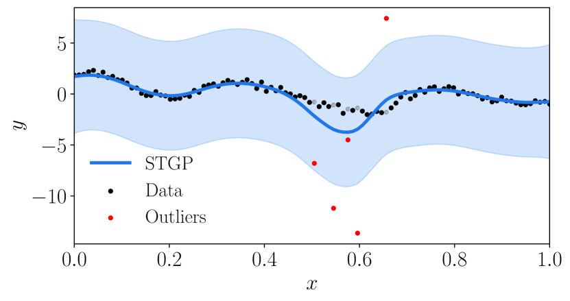
(a) Fitting STGP on Outlier Data. The hyperparameters obtained are: Lengthscale $\ell=0.118$, amplitude $\sigma_{\kappa}=3.438$, observation noise $\sigma^{2}=2.842$.

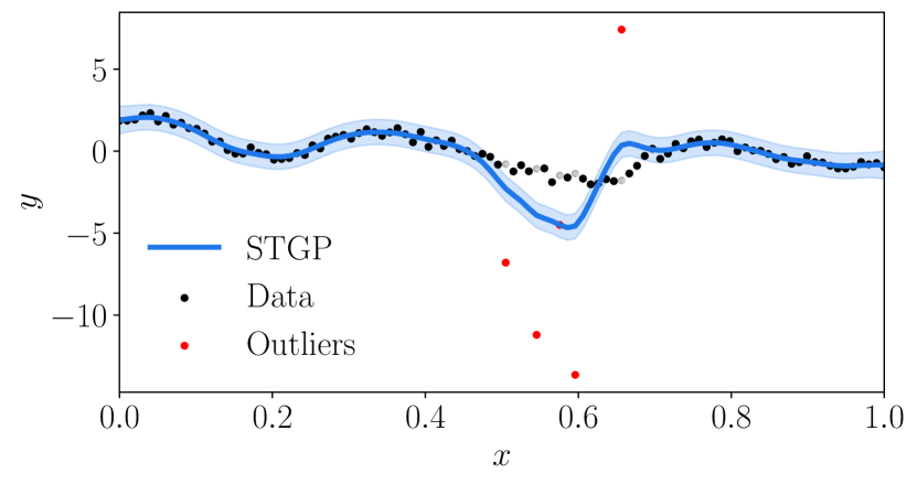
(b) Fitting STGP on Outlier-Free Data. The hyperparameters obtained are: Lengthscale $\ell=0.236$, amplitude $\sigma_{\kappa}=3.187$, observation noise $\sigma^{2}=0.055$.

Figure 9: Impact of outliers on hyperparameter optimisation with $\varphi$. The data is generated in the same way as for Figure 4 but with 100 data points instead and five outliers from a $\mathcal{N}(0,\sigma=10)$. Both models use a Matérn 3/2 kernel.

Improving ST-RCGP’s Hyperparameter Optimisation: Temporal Setting

For temporal data, we now show that when there are outliers in the training data and we are using the ST-RCGP algorithm, choosing $\varphi_{\text{GB}}$ from Section 3 as an objective function for hyperparameter optimisation is more reliable than using the regular $\varphi$. It is given by:

$$\varphi_{\text{GB}}(\bm{\theta}):=\sum_{k=1}^{n_{t}}w_{k}\left(\log|2\pi\mathbf{S}_{k}(\bm{\theta})|+\bm{\varepsilon}_{k}^{\top}(\bm{\theta})\mathbf{S}_{k}^{-1}(\bm{\theta})\bm{\varepsilon}_{k}(\bm{\theta})\right),$$

where definitions are as above with $n_{s}=1$, and the weights $w_{k}$ are the ones from the ST-RCGP. In Figure 10, we fit the ST-RCGP on contaminated data with both objective functions to the best of our ability (that is, we adapt the learning rate and the number of optimisation steps as best as we can to get optimal results). We observe that using $\varphi_{\text{GB}}$ improves the optimisation process drastically compared to using $\varphi$, since way fewer steps were necessary, and doing so allows obtaining reasonable hyperparameter values for inference.

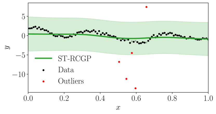
(a) Fitting ST-RCGP on Outlier Data With $\varphi$. The hyperparameters obtained are: Lengthscale $\ell=0.683$, amplitude $\sigma_{\kappa}=2.078$, observation noise $\sigma^{2}=1.909$. The optimisation process takes roughly 100 steps at a rate of 0.009 and is unstable (does not converge and produces infinite values if learning rate is increased).

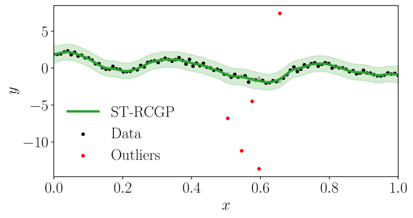
(b) Fitting ST-RCGP on Outlier Data With $\varphi_{\text{GB}}$. The hyperparameters obtained are: Lengthscale $\ell=0.112$, amplitude $\sigma_{\kappa}=4.162$, observation noise $\sigma^{2}=0.094$. The optimisation process takes roughly 25 steps at a rate of 0.2 and is considerably more stable.

Figure 10: Impact of objective function on ST-RCGP’s hyperparameter optimisation. The data is generated in the same way as for Figure 9. Both models use a Matérn 3/2 kernel and centering and shrinking function as specified in Section 3.

Improving ST-RCGP’s Hyperparameter Optimisation: Spatio-Temporal Setting

We turn our attention to spatio-temporal data and make the same point as in the previous paragraph, which is that choosing $\varphi_{\text{GB}}$ is more reliable than using the standard $\varphi$. We use the following objective:

$$\varphi_{\text{GB}}(\bm{\theta}):=\sum_{k=1}^{n_{t}}\tilde{w}_{k}\left(\log|2\pi\mathbf{S}_{k}(\bm{\theta})|+\bm{\varepsilon}_{k}^{\top}(\bm{\theta})\mathbf{S}_{k}^{-1}(\bm{\theta})\bm{\varepsilon}_{k}(\bm{\theta})\right),$$

where now, the representation $\tilde{w}_{k}(\mathbf{w}_{k})$ of the weights $\mathbf{w}_{k}$ at time step $t_{k}$ is given by:

$$\tilde{w}_{k}:=\frac{Q_{k,n_{s}}(\delta)}{\sum_{i=1}^{n_{t}}Q_{i,n_{s}}(\delta)},$$

where $Q_{k,n_{s}}(\delta)$ is the $\delta$-quantile of the weights $\mathbf{w}_{k}$. In this experiment, we choose $\delta=0.05$. The data we use is identical as for Section C.4, except that the outliers are only introduced at steps $k=2\;\text{and}\;6$, and the rest remains uncontaminated. As a performance metric, we use the cumulative mean absolute difference (CMAD) between our estimate of the latent function and the true latent function (not the observations), which is given by $\text{CMAD}=\sum_{k=1}^{n_{t}}\frac{1}{n_{s}}\sum_{j=1}^{n_{s}}|\mathbf{f}_{k,j}-\mathbf{\hat{f}}_{k,j}|$.

We fit the data with an ST-RCGP that has a Matérn 3/2 kernel, and a centering and shrinking function as specified in Section 3. We compare using $\varphi$ and $\varphi_{\text{GB}}$ and optimise for 30 training steps with an Adam optimiser with learning rate of 0.1. We run the process five times with newly sampled data and outliers, keeping the latent function and the distributions from which the data and outliers are sampled the same. We find that $\varphi$ yields CMAD values of $[1.9974,1.6703,1.9517,1.6100,1.7321]$, whereas $\varphi_{\text{GB}}$ produces CMAD values of $[0.4633,0.5385,0.5058,0.4479,0.5321]$. The $\varphi_{\text{GB}}$ objective yields substantially smaller CMAD values, and thus provides a more reliable hyperparameter objective function. We illustrate this in Figure 11, where we show three time steps of the first run (out of the five) for both objective functions.

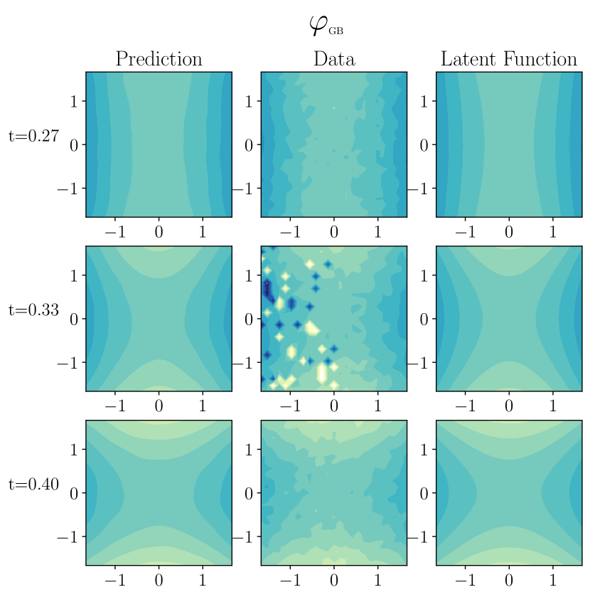
(a) Fitting ST-RCGP on Outlier Data with the Robust $\varphi_{\text{GB}}$.

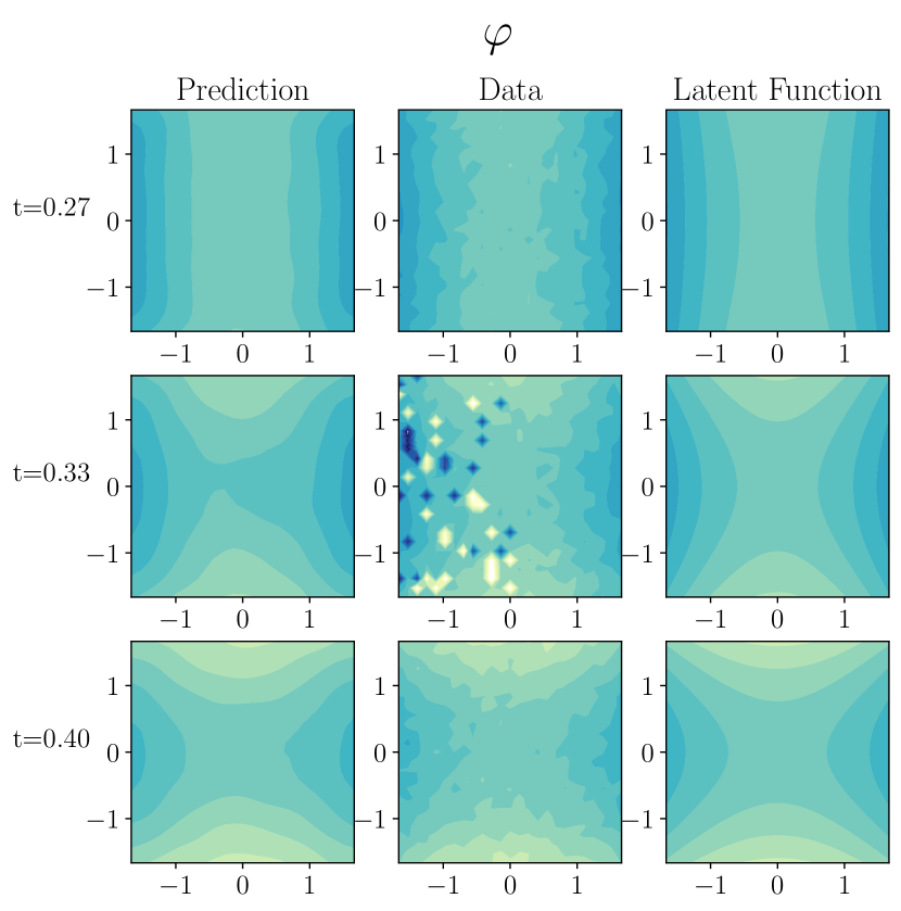
(b) Fitting ST-RCGP on Outlier Data with the Regular $\varphi$..

Figure 11: ST-RCGP Fits Using The Objective Functions $\varphi_{\text{GB}}$ and $\varphi$.

C.4 Synthetic Spatio-temporal Problem in Figure 1

A grid of size $n_{s}=25\times 25$ is produced and repeated through $n_{t}=10$ time steps between $t_{0}=0.2$ and $t_{f}=0.8$. We use a latent function $f(s_{1},s_{2},t)=\sin(2\pi t)s_{1}^{2}+\cos(2\pi t)s_{2}^{2}$ and generate additive noise from a $\mathcal{N}(0,\sigma^{2})$, where we set $\sigma=0.2$. At any time step, if a data point is located in the region $s_{1}<0$, with $10\%$ probability, we contaminate the data point with an outlier sampled from $U([-8,-6]\cup[6,8])$.

For both the STGP and ST-RCGP, we fit the data with the optimisation objective $\varphi$ and use de-contaminated data (original data without outliers) for the objective. We use the Adam optimiser with 20 training steps and 0.4 learning rate. The two algorithms use a Matérn 3/2 kernel. The ST-RCGP uses the adaptive centering and shrinking function from Section 3.

C.5 RCGP Issues from Section 2

The data is generated by adding noise sampled from a $\mathcal{N}(0,\sigma=0.5)$ to a latent function $f(x)=3\sin(2\pi x)$ on a temporal grid $x\in[0,1.4]$ with $n_{t}=80$ points. We substitute at 8 locations outliers drawn from a $\mathcal{N}(3,\sigma=0.2)$.

The RCGP optimisation process we use for kernel hyperparameters and observation noise is the one recommended in Altamirano et al. [2024]. Note that we conduct optimisation on the original data without outliers. We have three configurations: First, with constant prior mean $m(x)$ equal to the data average and $c=Q_{N}(0.9)$; second, with $m(x)=\sin(2\pi x)$ and $c=Q_{N}(0.9)$; third, with $m(x)=\sin(2\pi x)$ and $c=0.8$. All configurations use a Squared Exponential kernel and are separately optimised (that is, they do not necessarily share hyperparameters). Note that inference is conducted on data with outliers.

C.6 ST-RCGP Posterior when Varying $c$ and $\beta$

We generate $N=n_{t}=100$ data points from a GP prior with prior mean $m=0$ and Matérn 3/2 kernel with $\ell=0.2,\sigma_{\kappa}=2.0$. We add noise from a $\mathcal{N}(0,\sigma^{2})$ where $\sigma^{2}=0.25$. Outliers are generated by adding noise at 5 temporal locations drawn from a $\mathcal{N}(0,\sigma)$ with $\sigma=20$.

The ST-RCGP uses a Matérn 3/2 kernel with lengthscale $\ell=0.198$ and amplitude $\sigma_{\kappa}=3.01$. We use an adaptive centering function for all values of $\beta$ and $c$. Then, we perform inference with varying values of $\beta$ and $c$ to conduct a sensitivity analysis of those hyperparameters. The results are shown in Figure 12.

We notice that increasing $\beta$ will lead to overfitting the data. Conversely, decreasing $\beta$ too much yields under-confident uncertainty estimates. The middle ground is $\beta=\sigma/\sqrt{2}$, which yields mean and uncertainty estimates that are appropriate, thus supporting our selection of hyperparameters.

For $c$, Figure 12 shows that a lower $c$ will be more robust to outliers, but may as well over-inflate the uncertainty estimate. On the other hand, a $c$ that is too large will produce an algorithm closer to the STGP, which is not robust to outliers. Visibly, the adaptive choice for $c$ performs the best, confirming our choice of hyperparameter.

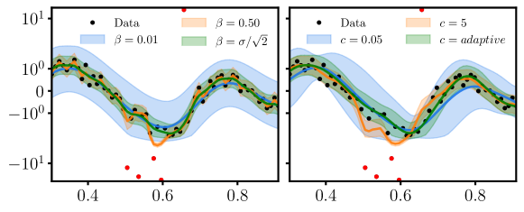
Figure 12: Impact of $c$ and $\beta$ on the posterior. We keep all parameters other than $\beta,c$ identical and choose $\mathbf{m}_{k}=\hat{\mathbf{f}}_{k}$. Outliers are highlighted in red. When $\beta$ increases (or decreases), the rate at which we learn from data increases (or decreases), and the confidence intervals narrow (or widen). When $c$ decreases, we increase robustness at the cost of larger posterior uncertainty. These tendencies support $\beta\propto\sigma$ and $c=\sqrt{\sigma^{2}+\sigma_{f}^{2}}$ where $\sigma_{f}$ is the standard deviation of the predictive filtering posterior $p(y_{k}|y_{1:k-1})$.

C.7 Choices of Centering Function in Special Cases

In Table 4, we highlight a few potential alternative choices other than ST-RCGP’s filtering predictive $\hat{\mathbf{f}}_{k}$ for the centering function depending on whether the data is temporal or spatio-temporal. Also, we demonstrate which choices of centering functions recover the STGP and RCGP. The below points briefly explain the relevant features of each choice:

• Data: This choice, which yields constant weights and thus recovers the STGP, implies that our best estimate of the center of the data is the current observation. Interestingly, if the observation is an outlier, this implies we center the algorithm around the outlier. This provides an intuitive understanding for why the STGP fails to be robust.

• Prior Mean: Choosing for our centering function the prior mean $m(\mathbf{x}_{k})$ recovers the RCGP (assuming a constant $c$ for the ST-RCGP). However, as previously explored in Section 4, this choice can yield poor results when the prior mean aligns with the outliers.

• Spatial Smoothing: This choice requires an additional hyperparameter (potentially many) that comes from $\bar{\mathbf{K}}_{s}$. The matrix $\bar{\mathbf{K}}_{s}$ dictates how much we want to smooth our data at time step $t_{k}$. This can be useful when there are unusual spatial structures in the data that $\bar{\mathbf{K}}_{s}$ can capture. Alternatively, when there are few time steps, the filtering predictive might not be the best estimate of the center of the data, in which case a good way to estimate the center that is more appropriate than a simple average is to use $\bar{\mathbf{K}}_{s}$.

• Temporal Smoothing: This centering function employs the same concept as the “Spatial Smoothing”. It requires a lookback period $n_{l}$ and weights $\psi_{i}$ that determine how important the datum at step $i$ is to estimate the center of the data at step $k$.

• Filtering Predictive: This is the choice we make in this paper for ST-RCGP and explained in Section 3. It involves no additional hyperparameters, and is our model’s best (and robust) prediction of $\mathbf{y}_{k}$ given past observations. These reasons are why we choose this option over the other for the ST-RCGP.

• Smoothed Predictive (S): Same concept as “Spatial Smoothing,” but the smoothing is applied on predictions instead of on the data.

• Smoothed Predictive (T): Same concept as “Temporal Smoothing,” but the smoothing is applied on predictions instead of on the data.

Table 4: Choice of Centering Function $\bm{\gamma}_{k}$ For Weights $\mathbf{w}_{k}$. $\psi_{i}$’s for $i=n_{l},...,k$ are normalised weights selected from the $n_{l}$-th past time step $t_{n_{l}}$ (lookback period). $\tilde{\mathbf{K}}_{s}\in\mathbb{R}^{n_{s}\times n_{s}}$ is a row-wise normalized kernel matrix.

Algorithm	Centering $\bm{\gamma}(\mathbf{x})$	Description
STGP	$\mathbf{y}_{k}$	Data
RCGP	$m(\mathbf{x}_{k})$	Prior Mean
ST-RCGP	$\tilde{\mathbf{K}}_{s}\mathbf{y}_{k}$	Spatial Smoothing
	$\sum_{i}\psi_{i}\mathbf{y}_{i}$	Temporal Smoothing
	$\hat{\mathbf{f}}_{k}\equiv\mathbf{H}\mathbf{m}_{k|k-1}$	Filtering Predictive
	$\tilde{\mathbf{K}}_{s}\hat{\mathbf{f}}_{k}$	Smoothed Predictive (S)
	$\sum_{i}\psi_{i}\hat{\mathbf{f}}_{i}$	Smoothed Predictive (T)

C.8 Experiments Showing we Fix Vanilla RCGP from Section 4

Data

We generate $n_{t}=200$ data points at evenly spaced inputs in $x=[0,1]$ from a GP with Matérn 3/2 kernel with lengthscale $\ell=0.1$ and amplitude $\sigma_{\kappa}^{2}=2$, and mean function $m(x)=2e^{-5x}$. The sample function $\mathbf{f}=(f_{1},\dots,f_{n_{t}})$ drawn is then centered: $\mathbf{f}\rightarrow\mathbf{f}-\bar{\mathbf{f}}$, where $\bar{\mathbf{f}}:=\frac{1}{n_{t}}\sum_{i=1}^{n_{t}}f_{i}$. Noise is added and drawn from a $\mathcal{N}(0,\sigma^{2})$ with $\sigma^{2}=0.25$. We contaminate the data with 10 outliers $|y_{i}^{c}|$ for $i=1,...,10$ sampled from a $\mathcal{N}(5,\sigma^{2}=1)$. These outliers replace the data at specified locations. We keep both the original data and the contaminated data for further tasks.

Fit

To fit the RCGP, we use the code from and follow Altamirano et al. [2024]. We choose a constant weight function equal to the mean of the data, and $c=Q_{N}(0.95)$ since there are 5% outliers. The hyperparameters are optimized on the original data (without outliers) since training RCGP on contaminated data would result in overfitting the outliers and unreliable predictions. However, RCGP predictions are made on contaminated data.

To fit the ST-RCGP, we use the Adam optimiser and the robust scoring objective $\varphi_{\text{GB}}$ from Section 3. The hyperparameter selection is as in Section 3. Our learning rate is 0.3 and number of optimisation steps is 70 (30 would be enough; we’ve used more to study convergence). In contrast to RCGP, the ST-RCGP is both training and predicting on contaminated data.

Coverage

The coverage values are computed given a prediction $\mu$ and standard deviation $\sigma$. For each quantile, we find a corresponding $z$-score, and determine the proportion of data points falling within $\mu\pm z\sigma$.

C.9 Experiments in Well-specified Settings from Section 4

We use the same dataset as in Section C.4, from which we can select the outlier-free data or the contaminated data. We use a Matérn 3/2 kernel for the GP prior. First, we perform hyperparameter optimisation on the dataset with outlier-free data. This involves 25 training steps using the Adam optimiser and a learning rate of 0.3. The criterion we use as our optimisation objective is the standard $\varphi$ (since there are no outliers). Second, we obtain the performance metrics for each model. This is done by generating new data as previously (from Section C.4). For each newly generated data, we compute statistical efficiency, RMSE and NLPD for each model. We take the average and standard deviation to report our metrics.

C.10 Experiments with Financial Crashes from Section 4

Twitter Flash Crash

We retrieve the ”close” data from the DJIA index on April 23th 2013 and the previous day. This amounts to 810 data points. We build an evenly spaced temporal grid from 0 to 1 with 810 points. The observations are then standardised.

The GP fit is implemented in Python’s sklearn package and uses a Matérn 3/2 kernel with amplitude $\sigma_{\kappa}=0.72$, lengthscale $\ell=0.0955$, observation noise $\sigma=0.02$, and prior mean $m=0$. The RCGP fit uses a Matérn 3/2 kernel with $\sigma_{\kappa}=1$, lengthscale $\ell=0.09$, a and a constant prior mean equal to the average of the data. Also, RCGP has $c=0.25$, since it offers a more robust posterior than $c=Q_{N}$. The ST-RCGP fit uses a Matérn 5/2 kernel with amplitude $\sigma_{\kappa}=1.$, lengthscale $\ell=0.1$, $\sigma^{2}=0.02$ and has an adaptive shrinking and centering function, as specified in Section 3. The RP fit is exactly the one from Ament et al. [2024] since it is obtained using the same code.

The execution time is computed post-optimisation of each method, since we wish to capture execution time at inference. Also, to avoid caching and establish a fair comparison, each model has a second instance specifically for inference-making that hasn’t observed data yet but has the optimised hyperparameters.

Index Futures with Synthetic Crash

The data is obtained from https://www.kaggle.com/c/caltech-cs155-2020/data. It captures an Index Futures price over time, measured at 500ms intervals. We select $N=46800$ data points, which amounts to a trading day. We built a temporal grid between 0 and 46800 and rescale it by 0.5 ($500\times 0.001$). The observations are then standardised. The crash induced aims to mimic the Twitter crash incident but with slightly more outliers. Therefore, we drop 8 data points by $[0.9995,0.9994,0.9992,0.996,0.994,0.998,0.998,0.9998]$ of their original value (not standardised) to create a V-shaped outlier region and add random noise to the drop sampled from a $\mathcal{N}(0,\sigma)$ for $\sigma=0.0001$. Note that the amplitude of this drop is roughly similar to that of the Twitter flash crash experiment.

The STGP has a Matérn 3/2 kernel with $\ell=6$, $\sigma_{\kappa}=6$, and observation noise $\sigma=0.14$. The ST-RCGP has a Matérn 3/2 kernel with $\ell=6.5$, $\sigma_{\kappa}=1$, and observation noise $\sigma=0.3$. It also uses an adaptive centering and shrinking function as in Section 3. The BayesNewton methods all use a Student-T likelihood with $\text{df}=6$ (degrees of freedom), except for the Laplace method which has $\text{df}=4$. They are also optimized following the code from Wilkinson et al. [2023].

The execution times are computed 5 times and evaluated on a new instance of the model’s class to avoid cashing issues. The one-step cost for each method is obtained by evaluating execution time for an increasing number of data points ($N=5,10,100,500,1000,2000,2500,...,35000,40000,46800$), and then performing linear regression. The slope corresponds to the one-step cost. The RMSE and NLPD standard deviations are obtained by repeating inference on a newly generated crash event a total of 20 times.

C.11 Experiments with Temperature Forecasting from Section 4

The data is from the Climate Research Unit (CRU) and is available at https://crudata.uea.ac.uk/cru/data/hrg/. We select latitude and longitude ranges of $[45,60]$ and $[-12,8]$ respectively, which amounts to $n_{s}=571$ spatial locations per time step. The data is monthly, starting in January 2022 and ending in December 2023, which is a total of $n_{t}=24$ time steps. This leads to $N=n_{t}\times n_{s}=11,991$ data points. We add 6 focussed outliers on a patch with latitudes and longitudes in $[51.25,53.25],[-3,-1]$ respectively. The outliers are drawn from a $\mathcal{N}(120,\sigma^{2})$ with $\sigma=10$. Before fitting the data, we pre-process it by standardising.

To fit the data, we use the standard objective $\varphi$ (since the data has been cleaned by the CRU beforehand, see Harris et al. [2020]) with Adam optimiser, 60 optimisation steps and 0.05 learning rate. Both the STGP and the ST-RCGP use a Matérn 3/2 kernel for the temporal and spatial kernels. For STGP, this yields the following hyperparameters: A Temporal amplitude of $\sigma_{\kappa_{t}}=0.76$, temporal lengthscale $\ell_{t}=2.51$, spatial amplitude $\sigma_{\kappa_{s}}=0.76$, spatial lengthscale $\ell_{s}=2.42$, and variance $\sigma^{2}=0.15$. For ST-RCGP, the hyperparameters are: A Temporal amplitude of $\sigma_{\kappa_{t}}=1.12$, temporal lengthscale $\ell_{t}=2.13$, spatial amplitude $\sigma_{\kappa_{s}}=0.82$, spatial lengthscale $\ell_{s}=2.34$, and variance $\sigma^{2}=0.069$.

References

- Aftab et al. [2019] W. Aftab, R. Hostettler, A. De Freitas, M. Arvaneh, and L. Mihaylova. Spatio-temporal Gaussian process models for extended and group object tracking with irregular shapes. IEEE Transactions on Vehicular Technology, 68(3):2137–2151, 2019.
- Altamirano et al. [2023] M. Altamirano, F.-X. Briol, and J. Knoblauch. Robust and scalable Bayesian online changepoint detection. In International Conference on Machine Learning, pages 642–663. PMLR, 2023.
- Altamirano et al. [2024] M. Altamirano, F.-X. Briol, and J. Knoblauch. Robust and conjugate Gaussian process regression. In International Conference on Machine Learning, pages 1155–1185. PMLR, 2024.
- Ament et al. [2024] S. Ament, E. Santorella, D. Eriksson, B. Letham, M. Balandat, and E. Bakshy. Robust Gaussian processes via relevance pursuit. Advances in Neural Information Processing Systems (to appear), 2024.
- Barp et al. [2019] A. Barp, F.-X. Briol, A. Duncan, M. Girolami, and L. Mackey. Minimum Stein discrepancy estimators. Advances in Neural Information Processing Systems, 32, 2019.
- Bauer et al. [2016] M. Bauer, M. Van der Wilk, and C. E. Rasmussen. Understanding probabilistic sparse Gaussian process approximations. Advances in Neural Information Processing Systems, 29, 2016.
- Bissiri et al. [2016] P. G. Bissiri, C. C. Holmes, and S. G. Walker. A general framework for updating belief distributions. Journal of the Royal Statistical Society: Series B (Statistical Methodology), 78(5):1103–1130, 2016.
- Dewaskar et al. [2023] M. Dewaskar, C. Tosh, J. Knoblauch, and D. B. Dunson. Robustifying likelihoods by optimistically re-weighting data. arXiv preprint arXiv:2303.10525, 2023.
- Drineas et al. [2005] P. Drineas, M. W. Mahoney, and N. Cristianini. On the Nyström method for approximating a gram matrix for improved kernel-based learning. Journal of Machine Learning Research, 6(12), 2005.
- Dupuis and Morgenthaler [2002] D. J. Dupuis and S. Morgenthaler. Robust weighted likelihood estimators with an application to bivariate extreme value problems. Canadian Journal of Statistics, 30(1):17–36, 2002.
- Duran-Martin et al. [2024] G. Duran-Martin, M. Altamirano, A. Shestopaloff, L. Sánchez-Betancourt, J. Knoblauch, M. Jones, F.-X. Briol, and K. P. Murphy. Outlier-robust Kalman filtering through generalised Bayes. In International Conference on Machine Learning, pages 12138–12171. PMLR, 2024.
- Duvenaud [2014] D. Duvenaud. Automatic model construction with Gaussian processes. PhD thesis, Apollo - University of Cambridge Repository, 2014.
- Field and Smith [1994] C. Field and B. Smith. Robust estimation: A weighted maximum likelihood approach. International Statistical Review/Revue Internationale de Statistique, pages 405–424, 1994.
- Fonseca et al. [2023] T. C. Fonseca, V. G. Lobo, and A. M. Schmidt. Dynamical non-Gaussian modelling of spatial processes. Journal of the Royal Statistical Society Series C: Applied Statistics, 72(1):76–103, 2023.
- Garnett [2023] R. Garnett. Bayesian optimization. Cambridge University Press, 2023.
- Ghosh and Basu [2016] A. Ghosh and A. Basu. Robust Bayes estimation using the density power divergence. Annals of the Institute of Statistical Mathematics, 68(2):413–437, 2016.
- Hamelijnck et al. [2021] O. Hamelijnck, W. Wilkinson, N. Loppi, A. Solin, and T. Damoulas. Spatio-temporal variational gaussian processes. Advances in Neural Information Processing Systems, 34:23621–23633, 2021.
- Harris et al. [2020] I. Harris, T. J. Osborn, P. Jones, and D. Lister. Version 4 of the cru ts monthly high-resolution gridded multivariate climate dataset. Scientific data, 7(1):109, 2020.
- Hartikainen and Särkkä [2010] J. Hartikainen and S. Särkkä. Kalman filtering and smoothing solutions to temporal Gaussian process regression models. In IEEE International Workshop on Machine Learning for Signal Processing, pages 379–384, 2010.
- Hartikainen et al. [2011] J. Hartikainen, J. Riihimäki, and S. Särkkä. Sparse spatio-temporal Gaussian processes with general likelihoods. In Artificial Neural Networks and Machine Learning, pages 193–200. Springer, 2011.
- Heaton et al. [2011] M. J. Heaton, M. Katzfuss, S. Ramachandar, K. Pedings, E. Gilleland, E. Mannshardt-Shamseldin, and R. L. Smith. Spatio-temporal models for large-scale indicators of extreme weather. Environmetrics, 22(3):294–303, 2011.
- Hensman et al. [2013] J. Hensman, N. Fusi, and N. D. Lawrence. Gaussian processes for big data. In Uncertainty in Artificial Intelligence, page 282, 2013.
- Huber [1981] P. J. Huber. Robust statistics. Wiley Series in Probability and Mathematical Statistics, 1981.
- Hyun et al. [2016] J. W. Hyun, Y. Li, C. Huang, M. Styner, W. Lin, H. Zhu, A. D. N. Initiative, et al. Stgp: Spatio-temporal Gaussian process models for longitudinal neuroimaging data. Neuroimage, 134:550–562, 2016.
- Hyvärinen [2005] A. Hyvärinen. Estimation of non-normalized statistical models by score matching. Journal of Machine Learning Research, 6(24):695–709, 2005.
- Jewson et al. [2018] J. Jewson, J. Q. Smith, and C. Holmes. Principles of Bayesian inference using general divergence criteria. Entropy, 20(6):442, 2018.
- Kalman [1960] R. E. Kalman. A new approach to linear filtering and prediction problems. Transactions of the ASME–Journal of Basic Engineering, 82(Series D):35–45, 1960.
- Key et al. [2021] O. Key, T. Fernandez, A. Gretton, and F.-X. Briol. Composite goodness-of-fit tests with kernels. In NeurIPS 2021 Workshop Your Model Is Wrong: Robustness and Misspecification in Probabilistic Modeling, 2021.
- Knoblauch et al. [2022] J. Knoblauch, J. Jewson, and T. Damoulas. An optimization-centric view on Bayes’ rule: Reviewing and generalizing variational inference. Journal of Machine Learning Research, 23(132):1–109, 2022.
- Krige [1951] D. G. Krige. A statistical approach to some basic mine valuation problems on the Witwatersrand. Journal of the Southern African Institute of Mining and Metallurgy, 52(6):119–139, 1951.
- Kupilik and Witmer [2018] M. Kupilik and F. Witmer. Spatio-temporal violent event prediction using Gaussian process regression. Journal of Computational Social Science, 1(2):437–451, 2018.
- Liu and Briol [2024] X. Liu and F.-X. Briol. On the robustness of kernel goodness-of-fit tests. arXiv:2408.05854, 2024.
- Lyu [2009] S. Lyu. Interpretation and generalization of score matching. In Proceedings of the Twenty-Fifth Conference on Uncertainty in Artificial Intelligence, UAI ’09, page 359–366, Arlington, Virginia, USA, 2009. AUAI Press. ISBN 9780974903958.
- Matsubara et al. [2022] T. Matsubara, J. Knoblauch, F.-X. Briol, and C. J. Oates. Robust generalised Bayesian inference for intractable likelihoods. Journal of the Royal Statistical Society Series B: Statistical Methodology, 84(3):997–1022, 2022.
- Matsubara et al. [2024] T. Matsubara, J. Knoblauch, F.-X. Briol, and C. J. Oates. Generalized bayesian inference for discrete intractable likelihood. Journal of the American Statistical Association, 119(547):2345–2355, 2024.
- Nickisch et al. [2018] H. Nickisch, A. Solin, and A. Grigorevskiy. State space Gaussian processes with non-Gaussian likelihood. In International Conference on Machine Learning, Proceedings of Machine Learning Research, pages 3789–3798, 2018.
- Pleiss et al. [2018] G. Pleiss, J. Gardner, K. Weinberger, and A. G. Wilson. Constant-time predictive distributions for Gaussian processes. In International Conference on Machine Learning, pages 4114–4123. PMLR, 2018.
- Rauch et al. [1965] H. E. Rauch, F. Tung, and C. T. Striebel. Maximum likelihood estimates of linear dynamic systems. AIAA Journal, 3(8):1445–1450, 1965.
- Reece and Roberts [2010] S. Reece and S. Roberts. An introduction to Gaussian processes for the Kalman filter expert. In International Conference on Information Fusion, pages 1–9, 2010.
- Reimann [2024] H. Reimann. Towards robust inference for Bayesian filtering of linear Gaussian dynamical systems subject to additive change. PhD thesis, Universität Potsdam, 2024.
- Santner et al. [2018] T. J. Santner, B. J. Williams, and W. I. Notz. The Design and Analysis of Computer Experiments. Springer, 2nd edition, 2018.
- Sarkka and Hartikainen [2012] S. Sarkka and J. Hartikainen. Infinite-dimensional Kalman filtering approach to spatio-temporal Gaussian process regression. In International Conference on Artificial Intelligence and Statistics, volume 22, pages 993–1001. PMLR, 2012.
- Särkkä and Solin [2019] S. Särkkä and A. Solin. Applied stochastic differential equations, volume 10. Cambridge University Press, 2019.
- Senanayake et al. [2016] R. Senanayake, S. O’Callaghan, and F. Ramos. Predicting spatio-temporal propagation of seasonal influenza using variational Gaussian process regression. In AAAI Conference on Artificial Intelligence, volume 30, 2016.
- Sinaga et al. [2024] M. A. Sinaga, J. Martinelli, and S. Kaski. Computation-aware robust Gaussian processes. In NeurIPS 2024 Workshop on Bayesian Decision-making and Uncertainty, 2024.
- Solin [2016] A. Solin. Stochastic differential equation methods for spatio-temporal Gaussian process regression. PhD thesis, Aalto University, 2016.
- Solin and Särkkä [2014] A. Solin and S. Särkkä. Gaussian quadratures for state space approximation of scale mixtures of squared exponential covariance functions. In IEEE International Workshop on Machine Learning for Signal Processing, pages 1–6. IEEE, 2014.
- Stein [1999] M. Stein. Interpolation of Spatial Data - Some Theory for Kriging. Springer Science+Business Media, 1999.
- Särkkä [2013] S. Särkkä. Bayesian Filtering and Smoothing. Institute of Mathematical Statistics Textbooks. Cambridge University Press, 2013.
- Tadayon and Rasekh [2019] V. Tadayon and A. Rasekh. Non-Gaussian covariate-dependent spatial measurement error model for analyzing big spatial data. Journal of Agricultural, Biological and Environmental Statistics, 24:49–72, 2019.
- Titsias [2009] M. Titsias. Variational learning of inducing variables in sparse Gaussian processes. In Artificial Intelligence and Statistics, pages 567–574. PMLR, 2009.
- Wang et al. [2013] C. Wang, X. Chen, A. Smola, and E. P. Xing. Variance reduction for stochastic gradient optimization. In Proceedings of the 26th International Conference on Neural Information Processing Systems-Volume 1, pages 181–189, 2013.
- Wilkinson et al. [2023] W. J. Wilkinson, S. Särkkä, and A. Solin. Bayes-Newton methods for approximate Bayesian inference with psd guarantees. Journal of Machine Learning Research, 24(83):1–50, 2023.
- Williams and Rasmussen [2006] C. K. Williams and C. E. Rasmussen. Gaussian processes for machine learning, volume 2. MIT press Cambridge, MA, 2006.
- Wilson and Nickisch [2015] A. Wilson and H. Nickisch. Kernel interpolation for scalable structured Gaussian processes (kiss-gp). In International conference on machine learning, pages 1775–1784. PMLR, 2015.
- Windham [1995] M. P. Windham. Robustifying model fitting. Journal of the Royal Statistical Society. Series B (Methodological), pages 599–609, 1995.
- Wu and Martin [2023] P.-S. Wu and R. Martin. A comparison of learning rate selection methods in generalized Bayesian inference. Bayesian Analysis, 18(1):105–132, 2023.
- Xu et al. [2022] J. Xu, J. L. Scealy, A. T. Wood, and T. Zou. Generalized score matching for regression. arXiv preprint arXiv:2203.09864, 2022.
- Yu et al. [2019] S. Yu, M. Drton, and A. Shojaie. Generalized score matching for non-negative data. Journal of Machine Learning Research, 20:1–70, 2019.