Hydrogen liquid-liquid transition from first principles and machine learning

Abstract

The molecular-to-atomic liquid-liquid transition (LLT) in high-pressure hydrogen is a fundamental topic touching domains from planetary science to materials modeling. Yet, the nature of the LLT is still under debate. To resolve it, numerical simulations must cover length and time scales spanning several orders of magnitude. We overcome these size and time limitations by constructing a fast and accurate machine-learning interatomic potential (MLIP) built on the MACE neural network architecture. The MLIP is trained on Perdew-Burke-Ernzerhof (PBE) density functional calculations and uses a modified loss function correcting for an energy bias in the molecular phase. Classical and path-integral molecular dynamics driven by this MLIP show that the LLT is always supercritical above the melting temperature. The position of the corresponding Widom line agrees with previous ab initio PBE calculations, which in contrast predicted a first-order LLT. According to our calculations, the crossover line becomes a first-order transition only inside the molecular crystal region. These results call for a reconsideration of the LLT picture previously drawn.

Introduction.

Pristine hydrogen is one of the most widely studied materials, both theoretically and experimentally [1]. Indeed, despite being made of the simplest atomic constituent, it exhibits a surprisingly rich phase diagram. The molecular-to-atomic transition happening upon liquid hydrogen compression is crucial for planetary science, in particular for understanding the interior of giant gas planets [2] and their magnetic fields [3]. This liquid-liquid transition (LLT) has been extensively investigated both experimentally [4, 5, 6, 7, 8, 9, 10, 11, 12, 13, 14] and via numerical simulations [15, 16, 17, 18, 19, 20, 21, 22, 23, 24, 25, 26, 27, 28, 29, 30, 31, 32, 33, 34, 35, 36, 37].

As is often the case for high-pressure hydrogen, experiments based on static [38, 39] and dynamic [40] compression give contrasting results, the dynamic experiments predicting a larger transition pressure. Uncertainty is also present in the numerical simulations. Results obtained with ab initio molecular dynamics (AIMD) using density functional theory (DFT) show large variability with respect to the choice of the exchange-correlation functional. For instance, the transition pressure can vary by $200$ GPa when including long-range Van der Waals corrections [41].

The nature of the LLT has been debated, with many first-principles simulations [15, 22, 21, 26, 27, 30, 35] suggesting a first-order LLT below a critical temperature $T_{c}$, based on the observation of kinks in the equation of state (EOS). Given the long correlations in both time and space expected near the transition, the outcome of first-principles molecular dynamics (MD) simulations using DFT or quantum Monte Carlo (QMC) methods has been questioned because of the short time scales and/or the small system sizes considered. This could be reflected in the large variability of the predicted $T_{c}$, which ranges from $T=4000$ K [27] to about $1250$ K for the most recent simulations [30].

In the past decade, large-scale simulations have been made possible by the introduction of machine learning interatomic potentials [42] (MLIPs). These provide results at much lower computational cost, once trained on datasets generated with ab initio methods. However, the derivation of an MLIP is a delicate step per se, possibly introducing a residual bias. A recent MLIP model, based on the NequIP [43] neural network (NN) and trained on DFT data, gave a $T_{c}$ value smaller than previous estimates [44]. This model has a pressure bias of about 5 GPa in the EOS, once compared with the corresponding ab initio predictions. Recent simulations based on another MLIP trained on the same DFT functional [34] suggested that the LLT is instead a smooth crossover, even though the accuracy of the model has been criticized [35, 45].

In this Letter, we present results for the LLT obtained with MACE [46], a framework combining an equivariant message-passing NN with high-body-order messages, which shows remarkable accuracy compared to other types of MLIPs. [47] In particular, we trained a MACE MLIP on the Perdew-Burke-Ernzerhof (PBE) functional and used it to study the nature of the LLT as a function of both system size and simulation length. Our results reveal a first-order transition between an atomic liquid and a molecular solid at low temperatures ($T<950$ K), due to the melting line proximity. At higher temperatures, our simulations indicate a crossover between molecular and atomic liquids in the thermodynamic limit.

MACE model from first principles.

To overcome the time and size limitations of ab initio simulations, while also retaining a high accuracy across the LLT, we constructed a MACE MLIP by applying a correction to the loss function usually minimized to find optimal parameters of the model. During the optimization, the loss and its gradients are evaluated on a subset of training configurations (”batch”) of dimension $N_{b}$. For the $\mu$-th configuration in the batch, having $N_{\mu}$ atoms, $E_{\mu}^{\textrm{pred}}$, $\mathbf{F}_{\mu,j}^{\textrm{pred}}$, and $\boldsymbol{\sigma}_{\mu}^{\textrm{pred}}$ are the total energy, the force acting on the $j$-th atom and the virial stress tensor, respectively, as predicted by the MLIP while $E_{\mu}^{\textrm{ref}}$, $\mathbf{F}_{\mu,j}^{\textrm{ref}}$, and $\boldsymbol{\sigma}_{\mu}^{\textrm{ref}}$ are the same quantities as calculated with DFT. A standard loss function $\mathcal{L}$ is the weighted sum of the mean squared errors (MSEs) of the different observables:

$$\mathcal{L} =w_{E}\frac{1}{N_{b}}\sum_{\mu=1}^{N_{b}}\left[\frac{1}{N_{\mu}}\left(E_{\mu}^{\textrm{pred}}-E_{\mu}^{\textrm{ref}}\right)\right]^{2}$$

$$+w_{F}\frac{1}{N_{b}}\sum_{\mu=1}^{N_{b}}\frac{1}{3N_{\mu}}\sum_{j=1}^{N_{\mu}}\sum_{\alpha=x,y,z}\left[F^{\textrm{pred}}_{\mu,j,\alpha}-F_{\mu,j,\alpha}^{\textrm{ref}}\right]^{2}$$

$$+w_{\sigma}\frac{1}{N_{b}}\sum_{\mu=1}^{N_{b}}\frac{1}{9}\sum_{\alpha=x,y,z}\sum_{\beta=x,y,z}\left[\sigma_{\mu,\alpha,\beta}^{\textrm{pred}}-\sigma_{\mu,\alpha,\beta}^{\textrm{ref}}\right]^{2},$$ (1)

where $w_{E}$, $w_{F}$, and $w_{\sigma}$ are tunable weights. However, when employing the loss in Eq. (1) to train the model , we noticed the appearance of unphysical molecular solid-like structures at high temperatures ($T\sim 1200$ K) during the dynamics. Even after the inclusion of these structures in the training set, the standard loss function still energetically favored these configurations (see the Supplemental Material (SM) for details [49]). The atomic phase, on the other hand, seemed to be described correctly.

With this in mind, we modified the loss function by including a term that penalizes a global energy bias in the prediction error on molecular configurations, thus improving the description of this phase. Specifically, we used the modified loss $\mathcal{L}^{\prime}=\mathcal{L}+\Delta\mathcal{L}$ with

$$\Delta\mathcal{L}=w_{E}\lambda\frac{1}{N_{\textrm{b}}}\left|\sum_{\mu\in\textrm{mol}}\frac{1}{N_{\mu}}\left(E^{\textrm{pred}}_{\mu}-E^{\textrm{ref}}_{\mu}\right)\right|,$$ (2)

where $\lambda$ is a parameter controlling the relative weight of the penalty with respect to the energy term of the standard loss function, and the sum only considers molecular configurations in a given training batch. To classify configurations as either atomic or molecular, we used a static criterion that solely depends on atomic positions: A configuration is classified as molecular if the first peak of its radial distribution function $g(r)$ (estimated by fitting the $g(r)$ with a Gaussian function for $r\in[0,1.3]$Å) is larger than a threshold, here set to $1.8$.

We observed that the models trained using $\mathcal{L}^{\prime}$ have a much smaller energy error for the molecular solid-like structures, which do not appear anymore during the dynamics at high temperatures. As a consequence of the modified loss, the energy error distribution on the training set is slightly altered, with relative energies between different types of structures in much better agreement with respect to the ab initio PBE reference values, as discussed in the SM.

To train the final MLIP, we compiled a dataset of $21\,812$ configurations, partitioned into training, test, and validation sets. We extracted $\sim 17\,000$ configurations of $128$ hydrogen atoms each from the MD simulations of Refs. [50] and [51] (see the SM for the density-temperature distribution of this set). An additional set of $3000$ 128-atoms configurations was selected from a series of AIMD simulations at lower temperatures (800 and 900 K). We also added $500$ snapshots with 256 and 512 atoms extracted from MD runs with early iterations of the MACE model. Finally, we included solid structures (see Ref. [52]) and $\sim 100$ low-temperature $96$-atoms configurations from Ref. [53]. To ensure consistency across the dataset, we recomputed energies, forces, and pressures at the PBE level, using the Quantum Espresso package [54, 55, 56]. A projector augmented-wave (PAW) pseudopotential [57] together with a $60$ Ry plane-waves cutoff was used. A sufficiently dense $\mathbf{k}$-point grid for each system size was employed to cure finite-size effects. For instance, we used a $4\times 4\times 4$ grid for the configurations with $128$ atoms.

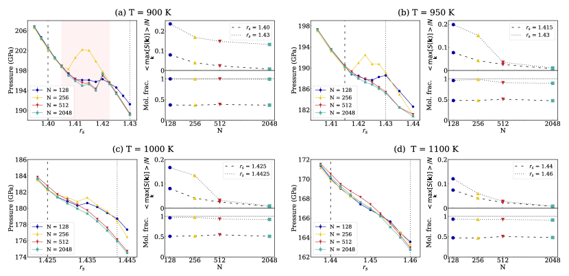
Figure 1: Results for MD simulations obtained with the MACE model for different temperatures: (a) $T=900$ K, (b) $T=950$ K, (c) $T=1000$ K, (d) $T=1100$ K. For each temperature, the left panel reports the EOS close to the LLT for the different system sizes. For $T=900$ K the red shaded area highlights the $r_{s}$ range for which hysteresis is observed at all values of $N$. The right panels show the average $\max_{\mathbf{k}}S(\mathbf{k})/N$ along the trajectory (top right) and the average molecular fraction $m$ (bottom right) as a function of the system size $N$ for two different values of the Wigner-Seitz radius $r_{s}$.

From this dataset, we extracted $280$ configurations for testing. From the remaining configurations, $95\%$ were used for training, and $5\%$ for validation. This last group of configurations is used during the training to assess the performance of the model. At the end of the optimization, the best model is selected as the one minimizing the loss on the validation set.

	RMSEE (meV/atom)	RMSEF (meV/Å)
Training	$2.2$	$116$
Validation	$2.1$	$118$
Test	$2.0$	$116$

Table 1: Root mean squared errors of the final MACE MLIP for the energy per atom ($\textrm{RMSE}_{E}$) and the forces ($\textrm{RMSE}_{F}$) on the training, validation, and test sets.

Table 1 reports the accuracy of this MACE model, measured by the root mean squared error (RMSE) on the energy per atom and the forces on the training, validation, and test sets. The test-set RMSE for the virial pressure is $\sim 1$ GPa. Compared to the MLIP proposed in Ref. [34], our model has an error on energy $6-7$ times smaller and is twice as accurate on forces. The recent NequIP model of Ref. [44] shows a very similar RMSE on energy, but has a $40\%$ larger RMSE on forces.

LLT simulations: finite-size scaling.

The computational efficiency of the MACE model enabled us to study the behavior of the LLT as a function of both temperature and system size. We ran MD simulations in the NVT ensemble using the LAMMPS code [58] interfaced with MACE. We considered systems with $N=128$, 256, 512, and 2048 hydrogen atoms treated as classical nuclei, and cubic supercells. We performed simulations as long as $0.6$ ns, about two orders of magnitude longer than what is usually achieved with AIMD. For the dynamics, we used a time step of $0.2$ fs and controlled the temperature via the stochastic velocity rescaling scheme [59], with a characteristic time of $\tau=0.1$ ps.

To accurately study the nature of the transition, we calculated the EOS of the system on a very dense grid of Wigner-Seitz radii $r_{s}$ in the vicinity of the LLT. The results are presented in Fig. 1 for four different temperatures in the $[900-1100]$ K range. From the EOS, we can identify three distinct regimes for the LLT: At the lowest temperature computed here, i. e., $T=900$ K (Fig. 1a), the model clearly predicts a first-order transition, signaled by the hysteresis present in the EOS for all system sizes. At $T=950$ K and $1000$ K (Figs. 1b and 1c, respectively), the EOS has a strong dependence on the system size in the transition region: the smaller systems (i. e., $N=128$ and 256) suggest again a first-order transition, while for larger $N$ the pressure plateau and hysteresis are missing. Finally, at $T\geq 1100$ K (Fig. 1d) the results indicate a smooth crossover, with a relatively small size dependence.

To characterize the LLT, the sole observation of the EOS is not sufficient, since it is known that for these transitions the density is not the primary order parameter [60]. In particular, we computed the stable molecular fraction [23, 30, 47] of the system, defined in this case as the average number of hydrogen pairs whose constituent atoms stay within a distance of $1.05$ Å for at least a time $\tau\sim 80$ fs.

The results corresponding to $r_{s}$ values slightly before/after the transition are also shown in Fig. 1. In all cases, the molecular fraction rapidly increases from values around $0.5$ to values close to $1$, signaling an atomic-to-molecular transition as $r_{s}$ increases.

Besides the stable molecular fraction, we also computed the structure factor, $S(\mathbf{k})$, to detect long-range spatial correlations, where $\mathbf{k}=\frac{2\pi}{L}(n_{1},n_{2},n_{3})$ , with $L$ being the side of the cubic simulation box and $n_{1},n_{2},n_{3}$ integer numbers. In particular, the maximum value of $S(\mathbf{k})$ can be used as a proxy for the formation of crystalline structures, with $\max_{\mathbf{k}}S(\mathbf{k})\propto N$ in a solid system in the thermodynamic limit. On the contrary, in a liquid, the rotational invariance implies that the contribution of each $\mathbf{k}$ to the $S(\mathbf{k})$ will stay constant for $N\rightarrow\infty$. The value of the average $\max_{\mathbf{k}}S(\mathbf{k})/N$ as a function of the number of particles is reported in the top right panels of Fig. 1. In the atomic phase, our simulations show that the system is a liquid at all temperatures. In the molecular region, the behavior of $\max_{\mathbf{k}}S(\mathbf{k})/N$ is instead strongly temperature dependent. Interestingly, the first-order transition observed in the EOS at $T=900$ K is accompanied by a non-vanishing value of $\max_{\mathbf{k}}S(\mathbf{k})/N$ in the thermodynamic limit, revealing a long-range spatial order of the molecular phase at this temperature (Fig. 1a). Moreover, at $T=950$ K and 1000 K, a large value of $\max_{\mathbf{k}}S(\mathbf{k})/N$ is present for $N=128$ and $256$ on the molecular side, then vanishing at larger $N$ (Figs. 1(b-c)). This suggests that the first-order transition seen in smaller systems is due to finite-size effects and it is between a molecular crystal and an atomic liquid. A genuine molecular liquid is instead observed for all system sizes at temperature $T\geq 1100$ K (Fig. 1d).

LLT simulations: finite-time effects.

Our finite-size scaling analysis highlights the importance of considering sufficiently large systems to obtain converged results for the LLT.

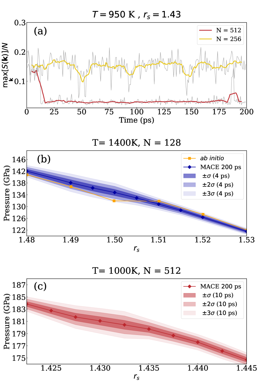
Figure 2: (a) Value of $\max_{\mathbf{k}}S(\mathbf{k})/N$ as a function of the simulation time for two systems, with $N=256$ and $N=512$ atoms, respectively, at temperature $T=950$ K and $r_{s}=1.43$. Colored lines represent running averages over a time window of $8$  ps. (b) Results for $200$ ps long simulations, $N=128$, $T=1400$ K and corresponding confidence intervals, estimated from a running average with time window $\tau_{\textrm{run}}=4$ ps. The AIMD result reported in Ref. [50] is also shown. (c) Same as (b) but with $N=512$, $T=1000$ K and $\tau_{\textrm{run}}=10$ ps.

This is further demonstrated in Fig. 2a, where the behavior of $\max_{\mathbf{k}}S(\mathbf{k})/N$ is plotted as a function of the simulation time for two sizes, namely $N=256$ and 512, at $T=950$ K and $r_{s}=1.43$. While the smaller system is in a solid-like state for the majority of the time, the system with $N=512$ occasionally crystallizes, as indicated by the two jumps of $\max_{\mathbf{k}}S(\mathbf{k})/N$ at the beginning and the end of the MD run, but it mostly remains liquid. This behavior not only confirms the size dependence already seen, but also shows that at least $10$ ps are necessary to melt the crystal for $N=512$, suggesting that $\sim 100$ ps are needed to have truly converged results near the transition.

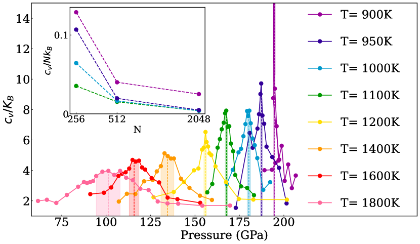
Figure 3: Specific heat per particle vs pressure along the isotherms, for $N=2048$ obtained with the MACE model. The shaded areas indicate the uncertainty in the peak position. In the inset, we report the size scaling of $c_{v}/k_{B}N$ for four different temperatures. The results confirm a first-order transition for $T=900$ K and a smooth crossover for higher temperatures in the thermodynamic limit.

To analyze the possibility that the kinks identified in the EOS of previous AIMD results originate from the short length of these simulations, we analyzed $0.2$ ns long trajectories obtained with the MACE model for values of $r_{s}$ close to the transition at different temperatures above our $T_{c}$. The results are shown in Figs. 2b and 2c for the system of $N=128$ at $T=1400$ K and the one of $N=512$ at $T=1000$ K, respectively. Using long trajectories, we computed the pressure running average using a variable-size time window $\tau_{\textrm{run}}$, corresponding to simulations times achievable by AIMD, e. g., $\tau_{\textrm{run}}\sim 10$ ps. The variance of the running average gives an idea of the variability of the estimated equilibrium pressure when running MD simulations of length equal to $\tau_{\textrm{run}}$. From Figs. 2b and 2c, we can notice that the estimated variance grows in the vicinity of the transition, and that the presence of a pressure plateau in the EOS can be understood as an artifact due to the lack of phase-space sampling.

For the smallest system ($N=128$, Fig. 2b), we also compared our results with the PBE AIMD ones reported in Ref. [50] at $T=1400$ K for the same size. The pressure plateau here is within the $3\sigma$ uncertainty region estimated from a running average of $4$ ps, slightly longer than the average length of the AIMD simulations. The results at lower temperature $T=1000$ K for a larger system of $512$ atoms (Fig. 2c) show that even a $10$ ps long dynamics can, in principle, produce artificial kinks of the size reported in the literature [21, 30]. Even though, in principle, this estimation depends on the algorithmic details, such as the choice of the thermostat, we do not expect this to change our conclusions.

Widom line.

Both the first-order transition and the crossover above the critical temperature $T_{c}$ can be further characterized by studying the behavior of the isochoric specific heat (i. e., the heat capacity per particle), $c_{v}=\frac{k_{B}}{NT^{2}}(\left\langle E^{2}\right\rangle-\left\langle E\right\rangle^{2})$, as a function of temperature, density, and system size. The results for $c_{v}$ obtained from simulations with $N=2048$ hydrogen atoms at temperatures up to $1800$ K are reported in Fig. 3. For each temperature, we estimated the location and value of the maximum. For temperatures between $900$ K and $1100$ K, we also studied the size scaling of the $c_{v}$ maximum, as shown in the inset of Fig. 3. In a first-order transition, the $c_{v}$ peak presents a divergence scaling like $\sim N$ in the thermodynamic limit [61]. As shown in the figure, linear scaling is observed at $T=900$ K, while the ratio $c_{v}/N$ tends to zero for higher temperatures. This is consistent with our EOS results locating the critical point between $T=900$ K and $T=950$ K. The position of the $c_{v}$ maximum at higher temperatures allows one to determine the Widom line in the supercritical region. The results are reported in Fig. 4. Our Widom line shows remarkable agreement with previous simulations of the LLT obtained with the PBE functional. In particular, our results well reproduce the ones reported in Ref. [21] for temperatures up to $1400$ K and those of Ref. [35] for higher temperatures, even though they do not agree on the LLT first-order character for $T\geq 900$ K.

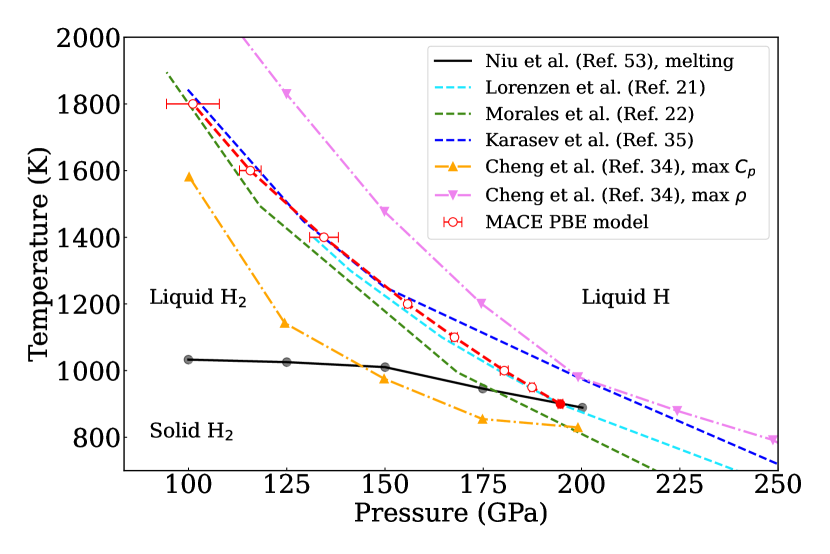
Figure 4: Classical PBE-LLT location as computed with different methods. AIMD results by Ref. [21] (light blue dashed line), Ref. [22] (green dashed line), Ref. [35] (blue dashed line). The results for the molecular-to-atomic crossover obtained with an NN MLIPs by Ref. [34] are reported with orange and violet markers, corresponding to the maximum of the isobaric specific heat and density, respectively. The black markers and line indicate the recently proposed PBE melting line by Ref.[53], obtained with an NN MLIP and the two-phase method. The MACE model results are indicated with red markers. The filled point at $T=900$ K indicates the first-order character of the transition, while the empty points correspond to the location of the Widom line given by the $c_{v}$ maximum (see Fig. 3).

Conclusions.

Enabled by an accurate and efficient MLIP based on the MACE architecture, we show that the LLT between molecular and atomic hydrogen is always supercritical above the melting temperature. For this, we performed NVT MD simulations in a temperature range between $900$ K and $1800$ K of systems with up to $2048$ hydrogen atoms and simulation times of up to $600$  ps. We preserved the ab initio PBE quality of the MACE model across the transition by virtue of a modified loss function, yielding consistent energy differences between atomic and molecular configurations.

For temperatures above $900$ K, the MACE model predicts a proper LLT in the thermodynamic limit ($N\geq 512$), which turns out to be a smooth crossover. Up to $T=1000$ K, defective crystal structures are observed for small systems due to strong finite-size effects, giving rise to a first-order transition that disappears as $N$ increases.

At the lowest temperature ($900$ K), the model predicts a first-order transition in the thermodynamic limit. The structure factor analysis reveals the presence of long-range spatial order in the molecular phase, showing that this is a transition between a molecular solid-like system, frustrated by the cubic cell, and an atomic liquid. This transition point lies exactly on the PBE melting line of Ref. [53] (see Fig. 4), calculated with an NN MLIP obtained using the DeePMD package [62], suggesting that the LLT might become first-order inside the crystal region for $T\leq 900$ K.

The physical picture provided by the MACE model qualitatively agrees with Ref. [34] on the supercritical nature of the LLT, even though their model could not accurately reproduce the crystallization regime, and predicted a Widom line (estimated from the maximum of the isobaric specif heat $c_{p}$ ) far from the AIMD results (see Fig. 4). The first-order character of the transition observed in other studies may be explained by the large fluctuations expected close to the Widom line, which could lead to the incorrect identification of density jumps and pressure plateaux in the EOS for too short simulation times. Additional path integral MD simulations carried out with the MACE model indicate that the conclusions about the crossover nature of the LLT are not changed by the inclusion of nuclear quantum effects, as reported in the SM [49].

These results urgently call for a reinvestigation of the LLT using ab initio methods beyond DFT, such as QMC. The $\Delta$-learning scheme [50, 51] combined with the present MACE model taken as baseline could allow one to access unprecedented system sizes and simulation lengths, by extending this work to QMC-based MLIP applications.

Data availability.

A version of the MACE code implementing the modified loss function employed in this work can be found at [63]. The model, training set, and simulation results are available at [64].

References

- Bonitz et al. [2024] M. Bonitz, J. Vorberger, M. Bethkenhagen, M. P. Böhme, D. M. Ceperley, A. Filinov, T. Gawne, F. Graziani, G. Gregori, P. Hamann, S. B. Hansen, M. Holzmann, S. X. Hu, H. Kählert, V. V. Karasiev, U. Kleinschmidt, L. Kordts, C. Makait, B. Militzer, Z. A. Moldabekov, C. Pierleoni, M. Preising, K. Ramakrishna, R. Redmer, S. Schwalbe, P. Svensson, and T. Dornheim, Physics of Plasmas 31, 110501 (2024).
- Helled et al. [2020] R. Helled, G. Mazzola, and R. Redmer, Nature Reviews Physics 2, 562 (2020).
- Connerney et al. [2017] J. E. P. Connerney, M. Benn, J. B. Bjarno, T. Denver, J. Espley, J. L. Jorgensen, P. S. Jorgensen, P. Lawton, A. Malinnikova, J. M. Merayo, S. Murphy, J. Odom, R. Oliversen, R. Schnurr, D. Sheppard, and E. J. Smith, Space Science Reviews 213, 39 (2017).
- Weir et al. [1996] S. T. Weir, A. C. Mitchell, and W. J. Nellis, Phys. Rev. Lett. 76, 1860 (1996).
- Fortov et al. [2007] V. E. Fortov, R. I. Ilkaev, V. A. Arinin, V. V. Burtzev, V. A. Golubev, I. L. Iosilevskiy, V. V. Khrustalev, A. L. Mikhailov, M. A. Mochalov, V. Y. Ternovoi, and M. V. Zhernokletov, Phys. Rev. Lett. 99, 185001 (2007).
- Dzyabura et al. [2013] V. Dzyabura, M. Zaghoo, and I. F. Silvera, Proceedings of the National Academy of Sciences 110, 8040 (2013).
- Ohta et al. [2015] K. Ohta, K. Ichimaru, M. Einaga, S. Kawaguchi, K. Shimizu, T. Matsuoka, N. Hirao, and Y. Ohishi, Scientific Reports 5, 16560 (2015).
- Knudson et al. [2015] M. D. Knudson, M. P. Desjarlais, A. Becker, R. W. Lemke, K. R. Cochrane, M. E. Savage, D. E. Bliss, T. R. Mattsson, and R. Redmer, Science 348, 1455 (2015).
- McWilliams et al. [2016] R. S. McWilliams, D. A. Dalton, M. F. Mahmood, and A. F. Goncharov, Phys. Rev. Lett. 116, 255501 (2016).
- Zaghoo et al. [2016] M. Zaghoo, A. Salamat, and I. F. Silvera, Phys. Rev. B 93, 155128 (2016).
- Zaghoo and Silvera [2017] M. Zaghoo and I. F. Silvera, Proceedings of the National Academy of Sciences 114, 11873 (2017).
- Zaghoo et al. [2018] M. Zaghoo, R. J. Husband, and I. F. Silvera, Phys. Rev. B 98, 104102 (2018).
- Celliers et al. [2018] P. M. Celliers, M. Millot, S. Brygoo, R. S. McWilliams, D. E. Fratanduono, J. R. Rygg, A. F. Goncharov, P. Loubeyre, J. H. Eggert, J. L. Peterson, N. B. Meezan, S. L. Pape, G. W. Collins, R. Jeanloz, and R. J. Hemley, Science 361, 677 (2018).
- Jiang et al. [2020] S. Jiang, N. Holtgrewe, Z. M. Geballe, S. S. Lobanov, M. F. Mahmood, R. S. McWilliams, and A. F. Goncharov, Advanced Science 7, 1901668 (2020).
- Scandolo [2003] S. Scandolo, Proceedings of the National Academy of Sciences 100, 3051 (2003).
- Bonev et al. [2004] S. A. Bonev, B. Militzer, and G. Galli, Phys. Rev. B 69, 014101 (2004).
- Delaney et al. [2006] K. T. Delaney, C. Pierleoni, and D. M. Ceperley, Phys. Rev. Lett. 97, 235702 (2006).
- Vorberger et al. [2007] J. Vorberger, I. Tamblyn, B. Militzer, and S. A. Bonev, Phys. Rev. B 75, 024206 (2007).
- Holst et al. [2008] B. Holst, R. Redmer, and M. P. Desjarlais, Phys. Rev. B 77, 184201 (2008).
- Attaccalite and Sorella [2008] C. Attaccalite and S. Sorella, Phys. Rev. Lett. 100, 114501 (2008).
- Lorenzen et al. [2010] W. Lorenzen, B. Holst, and R. Redmer, Phys. Rev. B 82, 195107 (2010).
- Morales et al. [2010] M. A. Morales, C. Pierleoni, E. Schwegler, and D. M. Ceperley, Proceedings of the National Academy of Sciences 107, 12799 (2010).
- Tamblyn and Bonev [2010] I. Tamblyn and S. A. Bonev, Phys. Rev. Lett. 104, 065702 (2010).
- Mazzola et al. [2014] G. Mazzola, S. Yunoki, and S. Sorella, Nature Communications 5, 3487 (2014).
- Yang et al. [2015] J. Yang, C. L. Tian, F. S. Liu, L. C. Cai, H. K. Yuan, M. M. Zhong, and F. Xiao, Europhysics Letters 109, 36003 (2015).
- Pierleoni et al. [2016] C. Pierleoni, M. A. Morales, G. Rillo, M. Holzmann, and D. M. Ceperley, Proceedings of the National Academy of Sciences 113, 4953 (2016).
- Norman and Saitov [2017] G. E. Norman and I. M. Saitov, Doklady Physics 62, 294 (2017).
- Mazzola et al. [2018] G. Mazzola, R. Helled, and S. Sorella, Phys. Rev. Lett. 120, 025701 (2018).
- Tian et al. [2019] C. Tian, F. Liu, H. Yuan, H. Chen, and A. Kuan, The Journal of Chemical Physics 150, 204114 (2019).
- Geng et al. [2019] H. Y. Geng, Q. Wu, M. Marqués, and G. J. Ackland, Phys. Rev. B 100, 134109 (2019).
- Rillo et al. [2019] G. Rillo, M. A. Morales, D. M. Ceperley, and C. Pierleoni, Proceedings of the National Academy of Sciences 116, 9770 (2019).
- Hinz et al. [2020] J. Hinz, V. V. Karasiev, S. X. Hu, M. Zaghoo, D. Mejía-Rodríguez, S. B. Trickey, and L. Calderín, Phys. Rev. Res. 2, 032065 (2020).
- Bryk et al. [2020] T. Bryk, C. Pierleoni, G. Ruocco, and A. P. Seitsonen, Journal of Molecular Liquids 312, 113274 (2020).
- Cheng et al. [2020] B. Cheng, G. Mazzola, C. J. Pickard, and M. Ceriotti, Nature 585, 217 (2020).
- Karasiev et al. [2021] V. V. Karasiev, J. Hinz, S. Hu, and S. Trickey, Nature 600, E12 (2021).
- Bergermann et al. [2024] A. Bergermann, L. Kleindienst, and R. Redmer, The Journal of Chemical Physics 161, 234303 (2024).
- Gliaudelis et al. [2025] G. Gliaudelis, V. Lukyanchuk, N. Chtchelkatchev, I. Saitov, and N. Kondratyuk, The Journal of Chemical Physics 162, 024504 (2025).
- Goncharov et al. [1995] A. F. Goncharov, I. I. Mazin, J. H. Eggert, R. J. Hemley, and H.-k. Mao, Phys. Rev. Lett. 75, 2514 (1995).
- Bassett [2009] W. A. Bassett, High Pressure Research 29, 163 (2009).
- Nellis [2006] W. J. Nellis, Rep. Prog. Phys. 69, 1479 (2006).
- Morales et al. [2014] M. A. Morales, R. Clay, C. Pierleoni, and D. M. Ceperley, Entropy 16, 287 (2014).
- Behler [2016] J. Behler, The Journal of Chemical Physics 145, 170901 (2016).
- Batzner et al. [2022] S. Batzner, A. Musaelian, L. Sun, M. Geiger, J. P. Mailoa, M. Kornbluth, N. Molinari, T. E. Smidt, and B. Kozinsky, Nat. Commun. 13, 2453 (2022).
- Istas et al. [2024] M. Istas, S. Jensen, Y. Yang, M. Holzmann, C. Pierleoni, and D. M. Ceperley, arXiv preprint arXiv:2412.14953 (2024).
- Cheng et al. [2021] B. Cheng, G. Mazzola, C. J. Pickard, and M. Ceriotti, Nature 600, E15 (2021).
- Batatia et al. [2022] I. Batatia, D. P. Kovacs, G. Simm, C. Ortner, and G. Csanyi, in Advances in Neural Information Processing Systems, Vol. 35, edited by S. Koyejo, S. Mohamed, A. Agarwal, D. Belgrave, K. Cho, and A. Oh (Curran Associates, Inc., 2022) pp. 11423–11436.
- Bischoff et al. [2024] T. Bischoff, B. Jäckl, and M. Rupp, arXiv e-prints , arXiv:2409.13390 (2024).
- Note [1] For building the model, we used equivariant messages, a correlation order of , and a cutoff radius of Å.
- [49] See Supplemental Material at [URL will be inserted by publisher] for further details about the training of the MACE model, a comparison between the error distribution of two models trained using the standard and modified loss, an analysis of the defective solid found in our simulations, a discussion of the path integral molecular dynamics results, and a comparison between our results and those obtained from ab initio molecular dynamics. (see references [65, 50, 51, 53, 35, 66, 26, 67, 47] therein).
- Tirelli et al. [2022] A. Tirelli, G. Tenti, K. Nakano, and S. Sorella, Phys. Rev. B 106, L041105 (2022).
- Tenti et al. [2024] G. Tenti, K. Nakano, A. Tirelli, S. Sorella, and M. Casula, Phys. Rev. B 110, L041107 (2024).
- Monacelli et al. [2023] L. Monacelli, M. Casula, K. Nakano, S. Sorella, and F. Mauri, Nature Physics 19, 845 (2023).
- Niu et al. [2023] H. Niu, Y. Yang, S. Jensen, M. Holzmann, C. Pierleoni, and D. M. Ceperley, Phys. Rev. Lett. 130, 076102 (2023).
- Giannozzi et al. [2009] P. Giannozzi, S. Baroni, N. Bonini, M. Calandra, R. Car, C. Cavazzoni, D. Ceresoli, G. L. Chiarotti, M. Cococcioni, I. Dabo, A. D. Corso, S. de Gironcoli, S. Fabris, G. Fratesi, R. Gebauer, U. Gerstmann, C. Gougoussis, A. Kokalj, M. Lazzeri, L. Martin-Samos, N. Marzari, F. Mauri, R. Mazzarello, S. Paolini, A. Pasquarello, L. Paulatto, C. Sbraccia, S. Scandolo, G. Sclauzero, A. P. Seitsonen, A. Smogunov, P. Umari, and R. M. Wentzcovitch, J. Phys.: Condens.Matter 21, 395502 (2009).
- Giannozzi et al. [2017] P. Giannozzi, O. Andreussi, T. Brumme, O. Bunau, M. B. Nardelli, M. Calandra, R. Car, C. Cavazzoni, D. Ceresoli, M. Cococcioni, N. Colonna, I. Carnimeo, A. D. Corso, S. de Gironcoli, P. Delugas, R. A. DiStasio, A. Ferretti, A. Floris, G. Fratesi, G. Fugallo, R. Gebauer, U. Gerstmann, F. Giustino, T. Gorni, J. Jia, M. Kawamura, H.-Y. Ko, A. Kokalj, E. Küçükbenli, M. Lazzeri, M. Marsili, N. Marzari, F. Mauri, N. L. Nguyen, H.-V. Nguyen, A. O. de-la Roza, L. Paulatto, S. Poncé, D. Rocca, R. Sabatini, B. Santra, M. Schlipf, A. P. Seitsonen, A. Smogunov, I. Timrov, T. Thonhauser, P. Umari, N. Vast, X. Wu, and S. Baroni, J. Phys.: Condens.Matter 29, 465901 (2017).
- Giannozzi et al. [2020] P. Giannozzi, O. Baseggio, P. Bonfà, D. Brunato, R. Car, I. Carnimeo, C. Cavazzoni, S. de Gironcoli, P. Delugas, F. Ferrari Ruffino, A. Ferretti, N. Marzari, I. Timrov, A. Urru, and S. Baroni, J. Chem. Phys. 152, 154105 (2020).
- [57] H.pbek-jpaw_psl.1.0.0.UPF pseudopotentials available at http://pseudopotentials.quantum-espresso.org/legacy_tables/ps-library/h.
- Thompson et al. [2022] A. P. Thompson, H. M. Aktulga, R. Berger, D. S. Bolintineanu, W. M. Brown, P. S. Crozier, P. J. in ’t Veld, A. Kohlmeyer, S. G. Moore, T. D. Nguyen, R. Shan, M. J. Stevens, J. Tranchida, C. Trott, and S. J. Plimpton, Computer Physics Communications 271, 108171 (2022).
- Bussi et al. [2007] G. Bussi, D. Donadio, and M. Parrinello, The Journal of Chemical Physics 126, 014101 (2007).
- Tanaka [2020] H. Tanaka, The Journal of Chemical Physics 153, 130901 (2020).
- Binder [1987] K. Binder, Reports on Progress in Physics 50, 783 (1987).
- Zeng et al. [2023] J. Zeng, D. Zhang, D. Lu, P. Mo, Z. Li, Y. Chen, M. Rynik, L. Huang, Z. Li, S. Shi, Y. Wang, H. Ye, P. Tuo, J. Yang, Y. Ding, Y. Li, D. Tisi, Q. Zeng, H. Bao, Y. Xia, J. Huang, K. Muraoka, Y. Wang, J. Chang, F. Yuan, S. L. Bore, C. Cai, Y. Lin, B. Wang, J. Xu, J.-X. Zhu, C. Luo, Y. Zhang, R. E. A. Goodall, W. Liang, A. K. Singh, S. Yao, J. Zhang, R. Wentzcovitch, J. Han, J. Liu, W. Jia, D. M. York, W. E, R. Car, L. Zhang, and H. Wang, The Journal of Chemical Physics 159, 054801 (2023).
- [63] https://github.com/giacomotenti/mace.
- Tenti et al. [2025] G. Tenti, B. Jäckl, K. Nakano, M. Rupp, and M. Casula, Additional data for ”hydrogen liquid-liquid transition from first principles and machine learning” (2025).
- Kingma and Ba [2014] D. P. Kingma and J. Ba, arXiv e-prints , arXiv:1412.6980 (2014).
- Momma and Izumi [2008] K. Momma and F. Izumi, Journal of Applied Crystallography 41, 653 (2008).
- Mouhat et al. [2017] F. Mouhat, S. Sorella, R. Vuilleumier, A. M. Saitta, and M. Casula, J. Chem. Theory Comput. 13, 2400 (2017).