A Null Space Compliance Approach for Maintaining Safety and
Tracking Performance in Human-Robot Interactions

Abstract

In recent years, the focus on developing robot manipulators has shifted towards prioritizing safety in Human-Robot Interaction (HRI). Impedance control is a typical approach for interaction control in collaboration tasks. However, such a control approach has two main limitations: 1) the end-effector (EE)’s limited compliance to adapt to unknown physical interactions, and 2) inability of the robot body to compliantly adapt to unknown physical interactions. In this work, we present an approach to address these drawbacks. We introduce a modified Cartesian impedance control method combined with a Dynamical System (DS)-based motion generator, aimed at enhancing the interaction capability of the EE without compromising main task tracking performance. This approach enables human coworkers to interact with the EE on-the-fly, e.g. tool changeover, after which the robot compliantly resumes its task. Additionally, combining with a new null space impedance control method enables the robot body to exhibit compliant behaviour in response to interactions, avoiding serious injuries from accidental contact while mitigating the impact on main task tracking performance. Finally, we prove the passivity of the system and validate the proposed approach through comprehensive comparative experiments on a 7 Degree-of-Freedom (DOF) KUKA LWR IV+ robot.

I Introduction

Industrial robots are increasingly attracting attention in sectors that require heavy labour due to their reliability, cost-effectiveness, and efficiency. However, not all manufacturing processes, such as automotive assembly and electronics manufacturing, can be fully automated without human intervention. Recently, advancements in safe HRI have been achieved with robot manipulators through various approaches: exteroceptive sensor-based methods, i.e. proximity sensor [1]; actuator-based approaches [2]; and software/controller-based solutions [3]. Among these methods, software/controller-based solutions are widely adopted in safe HRI applications due to their low cost, high versatility, and ease of implementation. Active compliant control, a method within this category, significantly contributes to safe HRI practices.

Active compliant control often involves techniques aimed at shaping the impedance or admittance of robots. These techniques are particularly valuable for ensuring safe HRI, especially when the robot is in contact with the environment [4]. Building upon this foundation, and recognizing the predominant use of Cartesian space control in industrial applications, Cartesian impedance control is introduced [5].

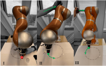
Figure 1: Interaction with robot while (I) holding the EE, (II) interacting with the robot body without affecting tracking, and (III) interacting using a handheld F/T sensor.

Specifically, classical Cartesian impedance-controlled robots maintain compliant behaviour by allowing deviations from the desired path in response to environmental obstacles or external forces, with interaction forces regulated by impedance parameters. However, post-interaction motion can become jerky if these parameters are not appropriately chosen, due to significant correction forces caused by large positional discrepancies during interactions. To address this issue, the correction force can be regulated by adjusting the impedance parameters through adaptive approaches [6]. However, these methods do not proactively change the robot’s trajectory to avoid unsafe interactions. In contrast, trajectory adaptation methods offer a more proactive solution by integrating trajectory adaptation with impedance control to ensure smooth transitions [7]. However, these approaches often introduce complexity and can cause undesirable delays during interactions. A more streamlined solution is to use a Dynamical System (DS)-based motion generator, which can instantly adapt to interactions without modifying the impedance characteristics [8]. In [9], a state-dependent DS motion generator is introduced, enabling trajectory adaptation to human interactions.

Achieving compliant motion at the EE is essential, while unintentional contact issues can also arise on the robot body [10]. This issue is particularly significant when using kinematically redundant manipulators for human-robot collaboration tasks. To address this challenge, exploiting redundancy to enable compliant behaviour in the joint space is a potential solution. A common approach for redundancy control is the null space projection method. In the literature, the null space motion can be regulated through optimization to guarantee the natural behaviour of robots during co-manipulation [11], or by hierarchical control to allow null space motion to resolve conflicts with higher priority tasks [12]. However, addressing the impact of unknown external interaction forces exerted on the robot body remains challenging. In [13], a null space impedance control is employed to react to the interaction forces acting on the robot body, complemented by an observer to compensate for Cartesian space errors. Nonetheless, this approach relies on accurate knowledge or estimation of the robot’s inertia matrix, which may not always be feasible in real-world settings.

To address these challenges, we aim to develop a new method that enables the robot to perform pre-defined tasks while exhibiting compliant behaviour to unknown interactions along the robot structure, ensuring tracking performance is unaffected without requiring the measurement or estimation of interaction forces and robot dynamics information. Our method enables the main task tracking in non-interaction situations while also allowing unknown interventions to interrupt EE motion, such as for tool changeover, then smoothly return to the desired path, as shown in Fig. 1 (I). To achieve these, we introduce an enhanced Cartesian impedance control method combined with a DS-based motion generator to generate interactable EE motions on-the-fly. Furthermore, we propose a novel null space impedance control strategy with joint friction torque compensation. This method efficiently extends compliant behaviour to the null space of the pre-defined main task, ensuring the tracking performance of the main task remains unaffected under unknown external interactions exerted on the robot body, as shown in Fig. 1 (II). The main contributions of this work are summarized as:

1. Introducing a modified Cartesian impedance control method combined with a DS-based motion generator, enhancing robot compliance during unknown physical interactions at the EE. This method ensures main task tracking and enables post-interaction path re-planning, allowing the EE to transition smoothly between interactions and the main task.

2. Introducing a novel null space impedance control method that enables the robot body to compliantly respond to unknown external interactions, without compromising the tracking performance of the main task. This method effectively dissipates external interaction energy in the null space, preserving tracking performance without requiring measurement or estimation of external forces, and robot dynamics information.

3. Demonstrating the proposed method’s passivity under conditions of unknown interaction forces and robot dynamics. This theoretically validates the effectiveness and safety of the proposed method for use in complex real-world HRI applications.

The proposed control scheme is evaluated under conditions of unknown interaction forces and robot dynamics. The results highlight its ability to achieve accurate, repeatable, interactable, interruptible motion and robot compliance.

The rest of this paper is organized as follows: Section II outlines the control objectives. Section III details the proposed control method and proves the passivity of the system. Section IV presents a series of comparative experiments and provides a numerical comparison. Section V discusses additional experimental findings, future directions, and concludes this work.

II Control Objective

In this work, we consider an $n$-DOF redundant serial robot manipulator. The dynamic model is expressed as,

$$M(q)\ddot{q}+C(q,\dot{q})\dot{q}+G(q)=\tau_{total}+\tau^{f}+\tau^{ext},$$ (1)

where ${q\in\mathbb{R}^{n}}$ denotes the joint configuration, ${M(q)\in\mathbb{R}^{n\times n}}$ is the inertia matrix. ${C(q,\dot{q})\in\mathbb{R}^{n\times n}}$ represents the Coriolis and centrifugal matrix, and ${G(q)\in\mathbb{R}^{n}}$ denotes the gravitational torques. ${\tau_{total}\in\mathbb{R}^{n}}$ denotes the total joint torque to be designed, ${\tau^{f}\in\mathbb{R}^{n}}$ denotes the joint frictional torque, and ${\tau^{ext}\in\mathbb{R}^{n}}$ denotes the unknown external interaction torque exerted on the robot joint. In the following, the dependency on joint configuration $(q,\dot{q})$ is omitted for the sake of brevity.

The total control torque $\tau_{total}$ in (1) can be designed as $\tau_{total}=G(q)+\tau^{c}+\tau^{n}$, where ${\tau^{c}\in\mathbb{R}^{n}}$ represents the Cartesian space joint control torque, ${\tau^{n}\in\mathbb{R}^{n}}$ represents the null space joint control torque, and $G(q)$ is the gravitational torque defined previously. It should be noted that the effect of gravitational torque can be accurately compensated in most industrial robot’s internal controllers.

Let $x_{d}=[p_{d}\;r_{d}]^{T}$, and $x=[p\;r]^{T}\in\mathbb{R}^{6}$ denote the desired and measured poses of the EE in 6D Cartesian space, in that $p_{d}=[p^{x}_{d},p^{y}_{d},p^{z}_{d}]^{T}$, and $p=[p^{x},p^{y},p^{z}]^{T}\in\mathbb{R}^{3}$ are the desired and measured positions, and $r_{d}=[\phi_{d},\theta_{d},\psi_{d}]^{T}$, and $r=[\phi,\theta,\psi]^{T}\in\mathbb{R}^{3}$ are the desired and measured orientations of the EE, respectively. Considering the total number of samples, $t$, each sample point of each vector is represented as $p_{d,i}^{x}$ and $p_{i}^{x}$ where $i\in\{1,2,\dots,t\}$.

In this work, our primary objectives are to: 1) maintain the tracking performance during interactions with the robot body, defined as,

$$\frac{\max\limits_{i=1}^{t}|p_{d,i}^{x}-p^{x}_{i}|}{\max\limits_{i=1}^{t}p_{d,i}^{x}-\min\limits_{i=1}^{t}p_{d,i}^{x}},$$ (2)

along the $x-$axis, as well as those for the $y-$ and $z-$ axes to remain at or below the level observed during the non-interaction scenario, 2) enable compliant behaviour of both the EE and the robot body when reacting to unknown external interactions, and 3) achieve objectives 1) and 2) without relying on the measurement or estimation of external interaction forces, as well as robot dynamics information. Details of non-interactive and interactive scenarios are given in Section IV.

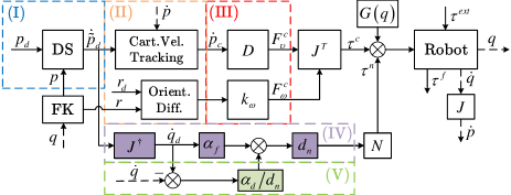
Figure 2: Control Diagram: (I) Cartesian motion generation, (II) tracking control, (III) modified Cartesian impedance control, (IV) proposed joint friction compensation, and (V) proposed null space impedance control.

III Methods

In this section, we present our control architecture in Fig. 2. The components include a Cartesian motion generator, tracking controllers, a modified Cartesian impedance controller, a proposed joint friction compensation approach, and a proposed null space impedance control strategy.

III-A Cartesian Space Motion Generation

III-A1 Motion Generator

In this subsection, we introduce a continuously differentiable state-dependent DS-based function $g(\mathscr{Z})$ in a feedback configuration, inspired by [9, 14]. Here, $\mathscr{Z}:=[\zeta_{1},...,\zeta_{s}]^{T}$ represents a set of state variables containing desired and measured Cartesian positions or orientations of the EE with $\zeta_{i}\in\mathbb{R}^{3}$ and $i\in\{1,2,\dots,s\}$. First, the DS stores the translational component $p_{d}$ of the desired Cartesian pose $x_{d}$ of a pre-defined task. The rotational component $r_{d}$ will be addressed in subsection III-A2. Second, to accommodate task-specific requirements, the stored $p_{d}$ can be transformed to the desired position using a function $g:\mathbb{R}^{3}\times\mathbb{R}^{3}\rightarrow\mathbb{R}^{3}$ describing the DS,

$${\tilde{p}}_{d}=g(p_{d},p;\Lambda),$$ (3)

where $p$ is obtained from the forward kinematics (FK), and $\Lambda=[\lambda_{1},\dots,\lambda_{t}]^{T}$, with $\lambda_{i}\in\mathbb{R}^{+}$ and $i\in\{1,2,\dots,t\}$, denotes the set of independent parameters utilized for state variable transformation. In the context of repetitive tasks, $\Lambda$ can be regarded as fixed parameters. Thirdly, taking the derivative of the desired position (3), the desired translational velocity $\dot{\tilde{p}}_{d}=[\dot{\tilde{p}}_{d}^{x},\dot{\tilde{p}}_{d}^{y},\dot{\tilde{p}}_{d}^{z}]^{T}\in\mathbb{R}^{3}$ can be expressed as

$$\dot{\tilde{p}}_{d}=\frac{d}{dt}g({p}_{d},p;\Lambda).$$ (4)

A specific application of (3) and (4) for a circle drawing task is provided in the experiment section. Note that in our design $\dot{\tilde{p}}_{d}$ serves as the reference input signal for the Cartesian velocity tracking controller as shown in Fig. 2 (II). In this setup, we utilize a Proportional–Derivative (PD) velocity tracking controller to ensure tracking performance,

$$\dot{p}_{c}=k_{p}(\dot{\tilde{p}}_{d}-\dot{p})+k_{d}(\ddot{\tilde{p}}_{d}-\ddot{p}),$$ (5)

where $\dot{p}_{c}=[\dot{p}^{x}_{c},\dot{p}^{y}_{c},\dot{p}^{z}_{c}]^{T}\in\mathbb{R}^{3}$ represents the controlled output of the Cartesian velocity tracking controller, $\dot{p}=[\dot{p}^{x},\dot{p}^{y},\dot{p}^{z}]^{T}\in\mathbb{R}^{3}$ represents the measured EE translational velocity. The term $\ddot{\tilde{p}}_{d}$ can be obtained by applying numerical differentiation to $\dot{\tilde{p}}_{d}$. Here, $k_{p}\in\mathbb{R}^{+}$ and $k_{d}\in\mathbb{R}^{+}$ represent the user-defined proportional and the derivative gain, respectively.

III-A2 Cartesian impedance control

In the previous subsection, we enabled the tracking of a task path by generating the desired translational velocity and implementing closed-loop velocity tracking. Based on this, we introduce a modified impedance controller to enable compliant behaviour. This controller derives the control torque from the result $\dot{p}_{c}$ of the Cartesian velocity tracking controller in (5).

Let $F^{c}=[F_{\upsilon}^{c}\;F_{\omega}^{c}]^{T}\in\mathbb{R}^{6}$ denote the Cartesian control force to be designed. The translational component of $F^{c}$, denoted by $F_{\upsilon}^{c}\in\mathbb{R}^{3}$, can be designed as,

$$F_{\upsilon}^{c}=D\>\dot{p}_{c}$$ (6)

where $D=\operatorname{diag}(d_{\upsilon}^{x},d_{\upsilon}^{y},d_{\upsilon}^{z})$, with $d_{\upsilon}^{x},d_{\upsilon}^{y},d_{\upsilon}^{z}\in\mathbb{R}^{+}$, denotes a diagonal damping matrix for translational motion in Cartesian space with positive entries. By reducing $D$, the EE can respond more compliantly to contacts from users or obstacles. This smooth response enables human coworkers to perform interactions (e.g., tool changeover) without requiring programmatic interruptions of motion.

The preceding focused on the translational motion to simplify the discussion. However, tasks such as polishing, which require maintaining the tool perpendicular to the surface, necessitate addressing the orientation control of the EE. The orientation control force $F_{\omega}^{c}\in\mathbb{R}^{3}$ can be formulated as,

$$F_{\omega}^{c}=K_{\omega}(r_{d}-r),$$ (7)

where $K_{\omega}=\operatorname{diag}(k_{\omega}^{\phi},k_{\omega}^{\theta},k_{\omega}^{\psi})$, with $k_{\omega}^{\phi},k_{\omega}^{\theta},k_{\omega}^{\psi}\in\mathbb{R}^{+}$, represents a diagonal stiffness matrix for the orientational motion of the EE with positive entries. Subsequently, the control torque $\tau^{c}\in\mathbb{R}^{n}$ can be expressed as,

$$\tau^{c}=J^{T}F^{c},$$ (8)

where $J\in\mathbb{R}^{6\times n}$ represents the Jacobian matrix of the $n$-DOF robot manipulator with a full rank of 6. Note that a more popular way to compute the orientation error in (7) is to convert the Euler angles to Quaternion representation. Further discussion regarding the orientation tracking accuracy is provided in Exp. A, as shown in Fig. 4 (c).

III-B Null Space Impedance Control

With the methods discussed in the previous subsections, we have enabled the EE to track the task path and safely interact with the users. This subsection focuses on allowing the robot body to respond to external interactions compliantly by controlling redundant DOFs, to reduce interference with Cartesian space motion. In other words, external energy exerted on the robot body can be effectively dissipated in the null space.

Let the relation between measured EE velocity $\dot{x}\in\mathbb{R}^{6}$ and measured joint velocity $\dot{q}\in\mathbb{R}^{n}$ be expressed as $\dot{x}=J\dot{q}$. A redundancy solution ($n>6$) to it is achieved through a null space projector $\dot{q}=J^{\dagger}\dot{x}+N\dot{q}$, where $J(q)^{\dagger}=J(q)^{T}(J(q)J(q)^{T})^{-1}\in\mathbb{R}^{n\times 6}$ denotes the pseudoinverse of $J(q)$. $N\in\mathbb{R}^{n\times n}$ is a null space projection matrix of $J(q)$, denoted as $N=I-J^{\dagger}J$, where $I\in\mathbb{R}^{n\times n}$ is an identity matrix. By utilizing the null space projection, redundant DOFs can be exploited to move within the null space of $J(q)$. This implies that the projection can be potentially used to project the external interaction forces to the null space. This is particularly valuable in scenarios where the robot interacts with its environment. In light of this, we propose a novel null space impedance control law formulated as,

$$\tau^{n}=Nd_{n}(\alpha_{f}\dot{q}_{d}+\frac{\alpha_{d}}{d_{n}}(\dot{q}_{d}-\dot{q})),$$ (9)

where $d_{n}\in\mathbb{R}^{+}$ represents the null space damping parameter. $\dot{q}_{d}=J(q)^{\dagger}\dot{\tilde{x}}_{d}\in\mathbb{R}^{n}$ denotes the desired joint velocity converted from the transformed desired velocity of the EE, denoted as $\dot{\tilde{x}}_{d}=[\dot{\tilde{p}}_{d}\mid\dot{r}_{d}]^{T}\in\mathbb{R}^{6}$. In practical implementation, the desired orientation velocity $\dot{r}_{d}$ of $\dot{\tilde{x}}_{d}$ is set to zero to maintain matrix integrity, with the orientation of the EE controlled by (7). The first term, $Nd_{n}\alpha_{f}\dot{q}_{d}$, functions as a feedforward compensation term for joint frictional torques, where $\alpha_{f}$ denotes the frictional gain parameter. By using the desired joint velocity $\dot{q}_{d}$, which provides a cleaner signal, and the null space projector $N$, the compensation is applied smoothly to the redundant DOFs. This enhances the joint responsiveness to external interactions. The second term $N\alpha_{d}(\dot{q}_{d}-\dot{q})$ utilizes null space projection to extend the joint motion into the null space of Cartesian space main tasks (e.g. polishing, buffing). Here, $\alpha_{d}$ represents the damping gain parameter that regulates the level of compliance. This term enables the redundant DOFs to respond compliantly to unknown external torque $\tau^{ext}$. The deviation between $\dot{q}$ and $\dot{q}_{d}$ caused by the external force generates damping torques through this term. The damping effect effectively dissipates external energy, reducing the impact on main task tracking performance. By combining these two terms, we ensure that external energy is exclusively dissipated through the joint damping effect, without being expended in resisting joint friction.

III-C Passivity Analysis

In this subsection, we analyze the passivity of the overall control system. We introduce a storage function consisting of three sub-system storage functions as follows: $S=S_{1}+S_{2}+S_{3}$, where $S_{1}=\frac{1}{2}\dot{e}_{q}^{T}M\dot{e}_{q}$ represents the kinetic energy associated with the joint velocity error induced by external interaction forces exerted on the robot body, $S_{2}=\frac{1}{2}{e}_{r}^{T}K_{\omega}{e}_{r}$ represents the spring potential energy of the orientation controller, and $S_{3}=\frac{1}{2}k_{d}\dot{e}_{p}^{T}D\dot{e}_{p}$ represents the energy dissipated due to the damping effect in the Cartesian impedance controller. Moreover, $\dot{e}_{q}=\dot{q}_{d}-\dot{q}$ denotes the joint velocity error, $e_{r}={r_{d}}-r$ represents the EE orientation error, $\dot{e}_{p}=\dot{\tilde{p}}_{d}-\dot{p}$ represents the EE translational velocity error.

Take the time derivative of $S$, we have,

$$\dot{S}=\dot{S}_{1}+\dot{e}_{r}^{T}K_{\omega}{e}_{r}+k_{d}\dot{e}_{p}^{T}D\ddot{e}_{p},$$ (10)

where $\dot{S}_{1}$ is given by,

$$\dot{S}_{1}=\dot{e}_{q}^{T}M\ddot{e}_{q}+\frac{1}{2}\dot{e}_{q}^{T}\dot{M}\dot{e}_{q}.$$ (11)

In HRI applications, due to safety requirements, task paths typically exhibit slow variations ($\ddot{q}_{d},\dot{q}_{d}\approx 0$). As a result, the contribution of Coriolis and centrifugal effects are negligible w.r.t. the external force, while inertial forces are insignificant w.r.t. that of the gravitational forces [11, 15]. Therefore, we assume $M\ddot{q}_{d}+C\dot{q}_{d}\approx 0$. Consequently, $M\ddot{e}_{q}$ in (11) can be decomposed and combined with (1) to be written as $M\ddot{e}_{q}=M\ddot{q}_{d}-M\ddot{q}=-C\dot{e}_{q}-\tau^{c}-\tau^{n}-\tau^{f}-\tau^{ext}$.

Substituting the above expression into (11), and consider skew symmetry of $(\dot{M}-2C)$, we have,

$$\dot{S}_{1} =\frac{1}{2}\dot{e}_{q}^{T}(\dot{M}-2C)\dot{e}_{q}-\dot{e}_{q}^{T}(\tau^{c}+\tau^{n}+\tau^{f}+\tau^{ext})$$

$$=-\dot{e}_{q}^{T}(\tau^{c}+\tau^{n}+\tau^{f}+\tau^{ext}).$$ (12)

By substituting (5)–(8) into (12), and considering $\dot{x}=[\dot{p}\mid\dot{r}]^{T}\in\mathbb{R}^{6}$, we obtain,

$$\dot{S}_{1} =-\dot{e}_{q}^{T}J^{T}\begin{bmatrix}F^{c}_{v}\\ F^{c}_{w}\end{bmatrix}-\dot{e}_{q}^{T}(\tau^{n}+\tau^{f}+\tau^{ext})$$

$$=-k_{p}\dot{e}_{p}^{T}D\dot{e}_{p}-k_{d}\dot{e}_{p}^{T}D\ddot{e}_{p}-\dot{e}_{r}^{T}K_{\omega}{e}_{r}$$

$$\quad-\dot{e}_{q}^{T}(\tau^{n}+\tau^{f}+\tau^{ext})$$

$$\leq-k_{d}\dot{e}_{p}^{T}D\ddot{e}_{p}-\dot{e}_{r}^{T}K_{\omega}{e}_{r}-\dot{e}_{q}^{T}(\tau^{n}+\tau^{f}+\tau^{ext}),$$ (13)

where the quadratic term $\dot{e}_{p}^{T}D\dot{e}_{p}$ is non-negative. Combine (10) with (13), we can cancel out the first two terms, i.e.,

$$\dot{S}\leq-\dot{e}_{q}^{T}(\tau^{n}+\tau^{f}+\tau^{ext}).$$ (14)

Substitute (9) into (14), and assume the friction torques can be approximately calculated by $-Nd_{n}\alpha_{f}\dot{q}$, we have,

$$\dot{S} \leq-\dot{e}_{q}^{T}(Nd_{n}(\alpha_{f}\dot{q}_{d}+\frac{\alpha_{d}}{d_{n}}(\dot{q}_{d}-\dot{q}))+\tau^{f})-\dot{e}_{q}^{T}\tau^{ext}$$

$$=-(d_{n}\alpha_{f}+\alpha_{d})\dot{e}_{q}^{T}N\dot{e}_{q}-\dot{e}_{q}^{T}\tau^{ext},$$ (15)

where the quadratic term $\dot{e}_{q}^{T}N\dot{e}_{q}$ is non-negative. The terms $d_{n}\alpha_{f}\geq 0$ and $\alpha_{d}\geq 0$ represent the coefficients of dissipated energy due to joint friction and the damping effect introduced by the null space impedance control law, respectively. Together, these terms facilitate energy dissipation within the system. Finally, we can write, $\dot{S}\leq-\dot{e}_{q}^{T}\tau^{ext}$, which ensures the passivity of the system w.r.t. the input-output pair $(-\tau^{ext},\dot{e}_{q})$. To evaluate the proposed methods, we discuss experiments in the following section.

IV Experimental Evaluation

The experiments are conducted on a 7-DOF KUKA LWR IV+ robot manipulator as shown in Fig. 3. The control algorithms are implemented on a remote Ubuntu PC with the Robot Operating System (ROS) framework. This remote PC establishes communication with the KUKA robot controller via UDP, utilizing the Fast Research Interface (FRI) with a sampling rate of 200 Hz. A $6$–axis ATI Gamma F/T sensor is attached to the EE for reference purposes. Throughout the experiments, the robot is controlled in joint impedance mode, and proper compensation for gravitational torques is ensured, including the effects of the F/T sensor and a lightweight 3D-printed tool. A handheld device incorporating the same ATI F/T sensor is used in robot body interaction experiments for reference purposes.

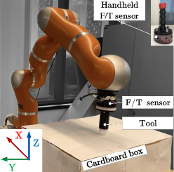
Figure 3: Experimental setup: 7-DOF robot arm with a 3D-printed tool, a mounted and a handheld F/T sensor for measuring interactive forces.

To evaluate the proposed method, we consider a circle-drawing task to represent a typical polishing pattern. This task involves tracing a circle of radius $\epsilon\in\mathbb{R}^{+}$ on the top flat surface of a cardboard box, centred at $O=[a,b,0]^{T}\in\mathbb{R}^{3}$ in Cartesian coordinates. The path is selected by the user to avoid kinematic singularities and joint limits. To accommodate task variations, the transformed desired position is,

$${\tilde{p}}_{d}={g}(p_{d},p;\Lambda):={\bar{\lambda}_{1}}\begin{bmatrix}\rho\cos(\delta)-a\\ \rho\sin(\delta)-b\\ 0\end{bmatrix}+\begin{bmatrix}a_{d}\\ b_{d}\\ {\bar{p}_{d}^{z}}\end{bmatrix}.$$ (16)

In this context, $\bar{\lambda}_{1}=\operatorname{diag}[\lambda_{1},\lambda_{1},1]$, where $\Lambda=\lambda_{1}=\frac{\epsilon_{d}}{\epsilon}\in\mathbb{R}^{+}$, represents the scaling factor. Here, $\epsilon_{d}$ denotes the radius of the desired circle. Consequently, the transformed position is represented in polar coordinate, where $\rho=\sqrt{({\Delta p^{x}})^{2}+({\Delta p^{y}})^{2}}$ and $\delta=atan2(\Delta p^{y},\Delta p^{x})\in[-\pi,\pi]$. Here, $\Delta p=[\Delta p^{x},\Delta p^{y},\Delta p^{z}]^{T}\in\mathbb{R}^{3}$ denotes the transformed position errors along the $x$–axis, $y$–axis, and $z$–axis, respectively. Specifically, $\Delta p$ is defined as $\Delta p=\bar{\lambda}_{1}^{-1}(p-O_{d})$, where $O_{d}=[a_{d},b_{d},\bar{p}_{d}^{z}]\in\mathbb{R}^{3}$ represents the translated center of the circle. Subsequently, the transformed desired translational velocity can be expressed by taking the time derivative of (16) as follows,

$$\dot{\tilde{p}}_{d} ={\bar{\lambda}_{1}}\begin{bmatrix}\dot{\rho}\cos(\delta)-\rho\dot{\delta}\sin(\delta)\\ \dot{\rho}\sin(\delta)+\rho\dot{\delta}\cos(\delta)\\ \dot{\tilde{p}}_{d}^{z}\end{bmatrix},$$ (17)

motivated by [9], $\dot{\rho}=k_{\rho}(\rho_{d}-\rho)$ represents the speed of convergence of $\rho$ to $\rho_{d}$, with $k_{\rho}\in\mathbb{R}^{+}$ being a gain parameter. The desired angular velocity, $\dot{\delta}\in\mathbb{R}^{+}$, can be selected by the user. The desired velocity of the $z$–axis motion can consequently be generated using a PD position controller expressed as,

$$\dot{\tilde{p}}_{d}^{z}=k_{P}({\bar{p}_{d}^{z}}-p^{z})+k_{D}({\dot{\bar{p}}_{d}^{z}}-\dot{p}^{z}),$$ (18)

where $k_{P}\in\mathbb{R}^{+}$ and $k_{D}\in\mathbb{R}^{+}$ represent the user-defined proportional and derivative gains, respectively.

The main task considered across three scenarios is tracing a circular path. The experiments include a non-interaction scenario (Exp. A), interaction with the EE (Exp. B, Exp. D), and interaction with the robot body (Exp. C – Exp. E). The non-interaction scenario serves as a baseline for evaluating tracking accuracy in 6D Cartesian space. In the EE interaction scenario, we examine the forces applied to the user while holding the EE, simulating a maintenance process. The robot body interaction scenario applies forces to the 4th joint along the $y$-axis relative to the base frame, mimicking external disturbances and environmental constraints. We experimentally compare our proposed method (Exp. C–2) with the baseline (Exp. C–1), a classical approach (Exp. D), and two state-of-the-art interaction force estimation methods [13, 16] (Exp. E). Table II summarizes the results.

IV-A Experiment A: Cartesian Path Tracking Without External Interaction

In this experiment, we evaluate the Cartesian path tracking accuracy in a non-interaction scenario using the proposed method. Here, we set up a scenario where the Tool Center Point (TCP) cyclically traces a circular path with a 10 cm radius on the top surface of a cardboard box. Initially, the joint configuration is approximately at $[0,2\pi/9,0,-\pi/2,0,5\pi/18,0]^{T}$ (rad) as shown in Fig. 3, the EE is positioned at the circle center. Additionally, the desired EE orientation $r_{d}$ is configured as $[\pi,0,\pi]^{T}$ (rad). This configuration ensures that the EE points vertically downward toward the surface. During motion, the yaw angle $\psi$ is constant relative to the base frame. Throughout the experiment, the robot remains free from external interaction forces, and the contact force along the $z$–axis of the EE is maintained close to zero, thus minimizing the effect of extraneous friction forces at the TCP. The control laws in (5)–(8), (9), and (17), (18) are utilized in this experiment. The control parameters, detailed in Table I, remain consistent across all experiments.

TABLE I: Control Parameters

Parameter	Value	Unit
$D$, $d_{n}$	$\operatorname{diag}(40,40,10)$, 5	N$\cdot$ s$/$m
$K_{\omega}$	$\operatorname{diag}(15,15,15)$	N$\cdot$ m$/$rad
$\alpha_{f}$, $\alpha_{d}$	1	–

Fig. 4 (a) demonstrates tracking accuracy remains under 7 mm in the $XY$ plane, with height error along the $z$–axis remaining under 3 mm. Minor fluctuations observed along the $z$–axis can be attributed to the uneven surface of the box.

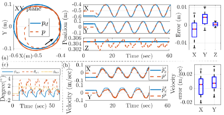
Figure 4: Non-interactive (Exp. A): (a) Position, (b) velocity, and (c) orientation trackings for the proposed method.

To ensure precise Cartesian path tracking, it is crucial to accurately track the generated desired velocity. Therefore, it is essential to evaluate the accuracy of the Cartesian velocity tracking along both the $x$–axis and $y$–axis. As presented in Fig. 4 (b), with a negligible error of approximately 1 cm$/$sec, the Cartesian velocity tracking controller demonstrates satisfactory performance, thereby contributing to the Cartesian position tracking accuracy. To further evaluate the orientation stability of the EE during motion, we illustrate the orientation error in Fig. 4 (c). The results demonstrate satisfactory performance, maintaining orientation error within $4^{\circ}$. The cyclical pattern of the error aligns with the orientation control employing solely stiffness control, outlined in (7).

IV-B Experiment B: Interaction on End-Effector

In this experiment, we investigate the interaction forces experienced by the user at the EE. The control laws applied are identical to those used in the preceding experiment. Following the setup from the previous experiment, the scenario involves the TCP cyclically tracing a circular path with a radius of 10 cm. During the motion, the user holds the EE for about 10 seconds, repeating this action four times. The random interaction points are as indicated in Fig. 5. Across four random interactions, the interaction forces range from 9 N to 18 N. The results demonstrate that the user can effortlessly execute the tool changeover procedure. In the last two interactions, the user demonstrates the ability to deviate the TCP from its desired path with slightly increased interaction forces.

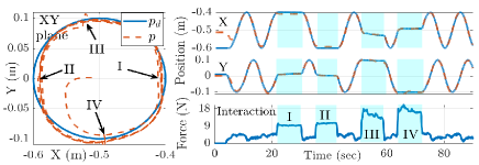
Figure 5: Interaction with the EE (Exp. B): position and measured interaction force using our proposed method. Shaded areas indicate periods of interaction.

IV-C Comparative Experiment C–1: Interaction on Robot Body Without Proposed Null Space Control Method

In this series of comparative experiments, we investigate the efficacy of the null space impedance control scheme introduced in subsection III-B. We aim to demonstrate the proposed null space controller enables the redundant DOFs to respond to unknown external interactions compliantly, thereby reducing interference with Cartesian space motion.

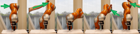
Figure 6: Interaction directions (indicated by green arrows).

In the first experiment, the proposed null space control scheme is omitted. This allows the Cartesian motion to be controlled by the DS motion generator as described in [9], combined with the tracking controllers and Cartesian impedance controller used in the preceding experiments as a baseline approach. The initial joint configuration is the same as in Exp. A. During pre-interaction periods, the tracking accuracy deteriorates compared to Fig. 4 (a). At 32 and 61 seconds, unknown interaction forces are applied on the 4^th joint. The directions of the interactions are indicated in Fig. 6. The duration of the interactions was approximately 2 and 4 seconds, respectively. The impact of interactions on the EE path tracking is indicated in Fig. 7 (a) (labelled with I and II). As seen, these interactions led to noticeable deviations from the desired path. The error along the $z$–axis ($\approx$ 2 cm) results in a loss of surface contact (Fig. 7 (b)).

Furthermore, to demonstrate the behaviour of the robot body, we depict the variations in joint angles in Fig. 7 (c). The $q_{1},q_{2},q_{3},q_{5},q_{6},q_{7}$ joints exhibit dynamic changes attributed to external interactions, with joints $q_{1},q_{2},q_{3},q_{5},q_{6}$ being particularly affected. Note that the variation of $q_{7}$ is excluded as it only pertains to the change of orientation of the EE. The fluctuations in joints indirectly affected by external forces (such as $q_{2}$ and $q_{6}$) indicate that the joints directly affected by external forces are inefficient in deviating from their initial positions to dissipate external energy. This inefficiency causes more joints to be affected, ultimately impacting tracking accuracy.

IV-D Comparative Experiment C–2: Interaction on Robot Body With Proposed Null Space Control Method

This comparative experiment introduces the proposed null space control into the system. The control laws applied remain consistent with those in Exp. A. Pre-interaction periods exhibit enhanced tracking accuracy, closely matching the performance depicted in Fig. 4 (a). We again apply unknown yet reasonably similar external forces (justified in Table II) to the 4^th joint around the 33 and 62 seconds. The interaction directions are labelled in Fig. 6. The interaction duration aligns with Exp. C–1. The impact of interactions on the EE tracking is indicated in Fig. 8 (a) (labelled with I and II). The Cartesian deviations induced by external interaction forces notably diminish compared to Fig. 7 (a, b), which closely match the accuracy of Exp. A.

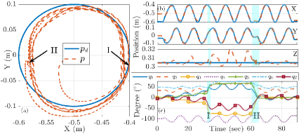
Figure 7: Performance of the baseline method [9] during robot body interaction (Exp. C–1): (a) Tracking performance, (b) $x$–, $y$–, and $z$–axes variations, and (c) joint variations.

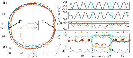
Figure 8: Performance of the proposed method during robot body interaction (Exp. C–2): (a) Tracking performance, (b) $x$–, $y$–, and $z$–axes variations, and (c) joint variations.

We further illustrate the variations in joint angles in Fig. 8 (c). When the interaction force acts on the 4^th joint, only $q_{1},q_{3}$, and $q_{5}$ respond to the external forces, and again $q_{7}$ is excluded from the discussion. This result demonstrates these joints compliantly deviate ($\approx$50^∘) from their initial positions, efficiently dissipating external energy within the null space. The robot’s responsiveness is also enhanced by compensating for joint friction. Thus, fewer joints are affected, leading to the tracking accuracy remaining unaffected.

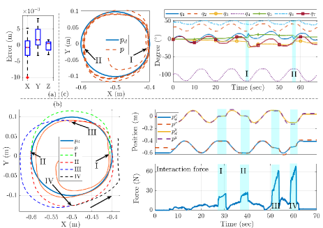
Figure 9: Performance of classical method [4] for comparison with (a) non-interaction (Exp. A), (b) EE interaction (Exp. B), and (c) robot body interaction (Exp. C).

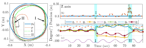
Figure 10: Performance of the Observer method [13] during robot body interaction (Exp. E): (a) Tracking performance, (b) $z$–axis variations, and (c) joint variations.

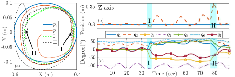
Figure 11: Performance of the RLSE method [16] during robot body interaction (Exp. E): (a) Tracking performance, (b) $z$–axis variations, and (c) joint variations.

TABLE II: Comparison of Interaction Forces on the Robot Body, Joint Deviations, and Tracking Accuracy.

	Classical[4]	Baseline [9]	Proposed	Observer [13]	RLSE [16]
Max force, I / II (N)	47/47	35/30	29/26	36/30	40/41
Joint deviation, I $\&$ II (∘)	$\approx$10	$\approx$45	$\approx$50	$\approx$45	$\approx$41
Pre-interaction NMAE, X/Y/Z (%)	5.0/4.2/1.5	10.3/6.0/2.2	6.4/4.5/1.0	8.8/5.4/1.3	10.1/4.7/1.4
Post-interaction NMAE, X/Y/Z (%)	5.1/8.7/1.5	12.3/11.0/5.7	5.9/6.2/1.1	23.0/11.0/15.8	22.0/14.4/19.7

IV-E Comparative experiment D: Classical Impedance Control

For a thorough evaluation, we compare a classical impedance control method presented in [4] with all prior experiments. The control law is given by $K_{c}(p_{d}-p)+D_{c}(\dot{p}_{d}-\dot{p})$, where $K_{c}=\operatorname{diag}(30,30,30)$ and $D_{c}=D$ represent the stiffness and damping matrices, respectively, selected to be consistent with the range used in previous experiments. EE orientation is controlled by (7). Fig. 9 (a) demonstrates Cartesian path tracking accuracy in the non-contact scenario as in Exp. A. The results indicate a similar level of tracking accuracy as in Fig. 4 (a). To maintain brevity, only the error signal boxplot is presented. However, when physical interactions are introduced, as in Exp. B and Exp. C the robot’s performance significantly degrades, as shown in Fig. 9 (b) and (c), respectively. In Fig. 9 (b), Exp. B is repeated, but the forces required to hold the tool in the current position increase sharply, by approximately three times, reaching a maximum of 60 N, which results in less interaction time ($\approx$ 3 sec). The interaction forces can continue to rise if the user does not release the tool. In Fig. 9 (c), Exp. C is repeated. The stiffness term reduces Cartesian deviations, but increases user-applied interaction forces (as justified in Table II). Joint deviations are limited ($\approx$$10^{\circ}$), the dissipation of external energy is therefore inefficient and results in less compliance and a more rigid behaviour.

IV-F Comparative Experiment E: Interaction on Robot Body with Null Space Interaction Estimation Methods

This section compares null space interaction handling performance using two interaction force estimation methods: a momentum-based observer (Fig. 10) from [13] and recursive least square estimation (RLSE) (Fig. 11) from [16]. The Cartesian control laws follow those in Exp. A, but the estimated null space interaction forces replace the proposed $\tau^{n}$ in (9). While the interaction directions match those in Exp. C, a slightly longer duration is needed to achieve comparable joint deviation due to increased resistance. Both methods exhibit similar tracking accuracy pre-interaction but fail to maintain main task tracking during and after interactions, particularly with significant $z$-axis errors ($\approx$5 cm), resulting in a loss of surface contact.

Table II provides a numerical comparison of the five methods, evaluating maximum interaction forces during two interactions, interaction-induced joint deviations, and the normalized maximum absolute error (NMAE), given by (2) along the $x$–, $y$–, and $z$–axes. Maximum interaction forces vary between 26 N and 47 N due to differences in null space compliance, with nearly identical forces observed across the two interactions for each method. Joint deviations, averaged for $q_{3}$ and $q_{5}$ across interactions, show similar values across methods (except for the classical method), indicating consistent interaction scenarios despite variations in resistance. The proposed method effectively dissipates external energy through redundant DOFs, reducing resistance for the user. In contrast, the classical method, being relatively rigid, offers accurate tracking but limited deviation. Pre-interaction tracking exhibits a mere 5$\%$ difference among methods, with the classical and proposed methods performing best. However, during and after interactions, the tracking accuracy of other methods degrades, with errors increasing by up to 18$\%$ along the $x$– and $z$–axes, highlighting the effectiveness and superiority of the proposed method.

V Discussion and Conclusion

The comparative results are satisfactory. The results in Table II represent the averages from multiple trials. The efficacy of the null space control law relies on the degrees of redundancy. Due to the constraints imposed by the main task, forces along the $y$–axis of the base frame and at or around the 4^th joint of the robot could be dissipated in the null space. Slight variations in maximum interaction forces reflect human’s variability. To avoid joint limit violations and singularities from aggressive interaction forces, the joint angles were kept within an optimal range. Future work will extend the permissible EE and robot body interaction forces while avoiding singularities and joint limits [17],[18].

This study introduced a control approach that enabled compliant interaction at both the EE and the robot body while maintaining main task tracking accuracy. The proposed method did not rely on measuring or estimating external interaction forces, nor on robot dynamics information. Its passivity was proven even in the presence of unknown interaction forces and robot dynamics. Comprehensive experimental validation on a KUKA LWR IV+ robot confirmed its efficacy and practical feasibility.

References

- [1] S. E. Navarro, S. Mühlbacher-Karrer, H. Alagi, H. Zangl, K. Koyama, B. Hein, C. Duriez, and J. R. Smith, “Proximity perception in human-centered robotics: A survey on sensing systems and applications,” IEEE Transactions on Robotics, vol. 38, no. 3, pp. 1599–1620, 2021.
- [2] Z.-Q. Yang and M. R. Kermani, “A computationally efficient hysteresis model for magneto-rheological clutches and its comparison with other models,” in Actuators, vol. 12, p. 190, MDPI, 2023.
- [3] M. Schumacher, J. Wojtusch, P. Beckerle, and O. Von Stryk, “An introductory review of active compliant control,” Robotics and Autonomous Systems, vol. 119, pp. 185–200, 2019.
- [4] N. Hogan, “Impedance control: An approach to manipulation: Part ii—implementation,” 1985.
- [5] C. Ott, Cartesian impedance control of redundant and flexible-joint robots. Springer, 2008.
- [6] F. J. Abu-Dakka and M. Saveriano, “Variable impedance control and learning—a review,” Frontiers in Robotics and AI, vol. 7, p. 590681, 2020.
- [7] Y. Lin, Z. Chen, and B. Yao, “Unified motion/force/impedance control for manipulators in unknown contact environments based on robust model-reaching approach,” IEEE/ASME Transactions on Mechatronics, vol. 26, no. 4, pp. 1905–1913, 2021.
- [8] S. M. Khansari-Zadeh and A. Billard, “Learning control lyapunov function to ensure stability of dynamical system-based robot reaching motions,” Robotics and Autonomous Systems, vol. 62, no. 6, pp. 752–765, 2014.
- [9] M. Khoramshahi, A. Laurens, T. Triquet, and A. Billard, “From human physical interaction to online motion adaptation using parameterized dynamical systems,” in 2018 IEEE/RSJ International Conference on Intelligent Robots and Systems (IROS), pp. 1361–1366, IEEE, 2018.
- [10] S. Haddadin, A. De Luca, and A. Albu-Schäffer, “Robot collisions: A survey on detection, isolation, and identification,” IEEE Transactions on Robotics, vol. 33, no. 6, pp. 1292–1312, 2017.
- [11] F. Ficuciello, L. Villani, and B. Siciliano, “Variable impedance control of redundant manipulators for intuitive human–robot physical interaction,” IEEE Transactions on Robotics, vol. 31, no. 4, pp. 850–863, 2015.
- [12] A. Dietrich and C. Ott, “Hierarchical impedance-based tracking control of kinematically redundant robots,” IEEE Transactions on Robotics, vol. 36, no. 1, pp. 204–221, 2019.
- [13] H. Sadeghian, L. Villani, M. Keshmiri, and B. Siciliano, “Task-space control of robot manipulators with null-space compliance,” IEEE Transactions on Robotics, vol. 30, no. 2, pp. 493–506, 2013.
- [14] K. Kronander and A. Billard, “Passive interaction control with dynamical systems,” IEEE Robotics and Automation Letters, vol. 1, no. 1, pp. 106–113, 2015.
- [15] F. Caccavale, B. Siciliano, and L. Villani, “The tricept robot: dynamics and impedance control,” IEEE/ASME transactions on mechatronics, vol. 8, no. 2, pp. 263–268, 2003.
- [16] Y. Lin, Z. Chen, and B. Yao, “Unified method for task-space motion/force/impedance control of manipulator with unknown contact reaction strategy,” IEEE Robotics and Automation Letters, vol. 7, no. 2, pp. 1478–1485, 2021.
- [17] S. Haddadin and E. Shahriari, “Unified force-impedance control,” The International Journal of Robotics Research, vol. 43, no. 13, pp. 2112–2141, 2024.
- [18] F. Dimeas, V. C. Moulianitis, C. Papakonstantinou, and N. Aspragathos, “Manipulator performance constraints in cartesian admittance control for human-robot cooperation,” in 2016 IEEE International Conference on Robotics and Automation (ICRA), pp. 3049–3054, IEEE, 2016.