Towards Fast Graph Generation via Autoregressive Noisy Filtration Modeling

Abstract

Graph generative models often face a critical trade-off between learning complex distributions and achieving fast generation speed. We introduce Autoregressive Noisy Filtration Modeling (ANFM), a novel approach that addresses both challenges. ANFM leverages filtration, a concept from topological data analysis, to transform graphs into short sequences of monotonically increasing subgraphs. This formulation extends the sequence families used in previous autoregressive models. To learn from these sequences, we propose a novel autoregressive graph mixer model. Our experiments suggest that exposure bias might represent a substantial hurdle in autoregressive graph generation and we introduce two mitigation strategies to address it: noise augmentation and a reinforcement learning approach. Incorporating these techniques leads to substantial performance gains, making ANFM competitive with state-of-the-art diffusion models across diverse synthetic and real-world datasets. Notably, ANFM produces remarkably short sequences, achieving a 100-fold speedup in generation time compared to diffusion models. This work marks a significant step toward high-throughput graph generation.

1 Introduction

Graphs are fundamental structures that model relationships in various domains, from social networks and molecular structures to transportation systems and neural networks. The ability to generate realistic and diverse graphs is crucial in many applications, such as drug discovery (Liu et al., 2018; Vignac et al., 2023), network simulation (Yu & Gu, 2019), and protein design (Ingraham et al., 2019). The space of drug-like molecules and protein conformations is, for practical purposes, infinite, limiting the effectiveness of in-silico screening of existing libraries (Polishchuk et al., 2013; Levinthal, 1969). Consequently, high-throughput graph generation—the task of efficiently creating new graphs that faithfully emulate properties similar to those observed in a given domain—has thus emerged as a critical challenge in machine learning and generative artificial intelligence (Gangwal et al., 2024; Grisoni et al., 2021).

Recent deep learning-based approaches, particularly autoregressive (You et al., 2018b; Liao et al., 2019; Kong et al., 2023) and diffusion models (Vignac et al., 2023; Bergmeister et al., 2024), have shown promise in generating increasingly realistic graphs. However, many current diffusion-based approaches rely on iterative refinement processes involving a large number of steps. This computational burden hinders their potential for high-throughput applications (Gentile et al., 2022; Gómez-Bombarelli et al., 2016; Polishchuk et al., 2013). While autoregressive models are more efficient during inference, they have underperformed in terms of generation quality. Moreover, they might be susceptible to exposure bias (Ranzato et al., 2016), where performance deteriorates as errors accumulate during sampling and a train-test discrepancy consequently arises.

Recent work has explored the use of topological data analysis, particularly persistent homology and filtration (Edelsbrunner et al., 2002; Zomorodian & Carlsson, 2005), for graph representation. A filtration provides a multi-scale view of a graph structure by constructing a nested sequence of subgraphs. This approach has shown potential in various graph analysis tasks, including classification and similarity measurement (O’Bray et al., 2021; Schulz et al., 2022). In the context of generative modeling, filtration-based representations have been used to develop more expressive tools for generative model evaluation (Southern et al., 2023). However, the application of filtration-based methods for graph generation remains unexplored. In this work, we propose filtrations as a generalization of graph sequence families used in prior autoregressive models (You et al., 2018b; Liao et al., 2019), offering a flexible framework to construct sequences for generation. Nonetheless, modeling filtration sequences in a naive manner remains prone to exposure bias.

To address this, we introduce Autoregressive Noisy Filtration Modeling (ANFM), a novel approach to fast graph generation that models noise-augmented filtration sequences autoregressively. To generate a target graph, our method produces a short sequence of increasingly dense and detailed intermediate graphs, which interpolate the target graph and the fully disconnected graph. Compared to diffusion models (Vignac et al., 2023; Bergmeister et al., 2024), ANFM requires fewer iterations during sampling, resulting in significantly faster inference speed. By adding noise to the filtration sequences, ANFM learns to simultaneously remove or add edges. As a result, it is able to recover from errors during sampling. Additionally, we further mitigate exposure bias with adversarial fine-tuning using reinforcement learning (RL). Our method offers a promising balance between efficiency and accuracy in graph generation, providing a 100-fold speedup over diffusion-based approaches, while substantially outperforming existing autoregressive models in terms of generation quality.

In summary, our contributions are as follows:

• We propose a novel autoregressive graph generation framework that leverages graph filtration. Our formulation generalizes the graph sequences used by previous autoregressive models that operate via node addition.

• We introduce a specialized autoregressive model architecture designed to operate on these graph sequences.

• We identify exposure bias as a potential challenge in autoregressive graph generation and propose noise augmentation and adversarial fine-tuning as effective strategies to mitigate this issue.

• We conduct ablation studies to evaluate the impact of different components within our framework, demonstrating that noise augmentation and adversarial fine-tuning substantially improve performance.

• Our empirical results highlight the strong performance and efficiency of our model compared to recent baselines. Notably, our model achieves inference speed 100 times faster than existing diffusion-based models.

2 Related Work

ANFM builds on the concept of graph filtration and incorporates noise augmentation. It is fine-tuned via reinforcement learning to mitigate exposure bias. In the following, we provide a brief overview of related graph generative models, approaches to address exposure bias, and applications of graph filtration.

Graph Generation.

GraphRNN (You et al., 2018b) made the first advances towards deep generative graph models by autoregressively generating nodes and their incident edges to build up an adjacency matrix row-by-row. In a similar fashion, DeepGMG (Li et al., 2018) iteratively builds a graph node-by-node. Liao et al. (2019) proposed a more efficient autoregressive model, GRAN, by generating multiple nodes at a time in a block-wise fashion, leveraging mixtures of multivariate Bernoulli distributions. GraphArm (Kong et al., 2023) introduced an autoregressive model that reverses a diffusion process in which nodes and their incident edges decay to an absorbing state. These models share the fact that they build graphs via node addition. Hence, they autoregressively generate an increasing sequence of induced subgraphs. In comparison, the subgraphs we consider in our work do not necessarily need to be induced. Moreover, ANFM may generate sequences that are not monotonic. In contrast to autoregressive node-addition methods, approaches by Goyal et al. (2020) and Bacciu et al. (2020) generate graphs through edge-addition following a pre-defined edge ordering. While this strategy bears similarities to our proposed filtration method, our approach distinctly differs by allowing for edge deletion as well as addition, leading to possibly non-monotonic sequences.

Diffusion models for graphs such as EDP-GNN (Niu et al., 2020) and GDSS (Jo et al., 2022), based on score matching, or DiGress (Vignac et al., 2023), based on discrete denoising diffusion (Austin et al., 2021), have emerged as powerful generators. However, they require many iterative denoising steps, making them slow during sampling. Hierarchical approaches (Bergmeister et al., 2024) and absorbing state processes (Chen et al., 2023) have subsequently been proposed to allow diffusion models to be scaled to large graphs. In contrast to the noise processes in denoising diffusion models, the filtration processes we consider are in general non-Markovian, necessitating a full autoregressive modeling.

Graph variational autoencoders (Kipf & Welling, 2016; Simonovsky & Komodakis, 2018) generate all edges at one time, thereby reducing computational costs during inference. However, these methods struggle to model complicated distributions and may fail in the presence of isomorphic nodes (Zhang et al., 2021). Generative adversarial networks (GANs) (Bojchevski et al., 2018; Cao & Kipf, 2018; Martinkus et al., 2022) are likelihood-free and avoid the node-orderings and graph matching algorithms required in autoregressive models and VAEs. However, they can be unstable during training and may suffer from issues such as mode collapse (Martinkus et al., 2022).

Exposure Bias.

Exposure bias (Bengio et al., 2015; Ranzato et al., 2016) refers to the train-test discrepancies autoregressive models face when they are exposed to their own predictions during inference. Errors may accumulate during sampling, leading to a distribution shift and degrading performance. To mitigate this phenomenon in natural language generation, Bengio et al. (2015) proposed a data augmentation strategy to expose models to their predictions during training. In a similar effort, Ranzato et al. (2016) proposed training in free-running mode using reinforcement learning to optimize sequence-level performance metrics. SeqGAN (Yu et al., 2017), which is the most relevant to our work, also trains models in free-running mode using reinforcement learning. Instead of relying on extrinsic metrics like Ranzato et al. (2016), it adversarially trains a discriminator to provide feedback to the generative model. GCPN (You et al., 2018a) adopts a hybrid framework for generating small molecules, combining adversarial and domain-specific rewards.

Graph Filtration.

Filtration is commonly used in the field of persistent homology (Edelsbrunner et al., 2002) to extract features of geometric data structures at different resolutions. Previously, graph filtration has mostly been used to construct graph kernels (Zhao & Wang, 2019; Schulz et al., 2022) or extract graph representations that can be leveraged in downstream tasks such as classification (O’Bray et al., 2021). While filtration has also been used for evaluating graph generative models (Southern et al., 2023), to the best of our knowledge, our work presents the first model that directly leverages filtration for generation.

3 Background

In the following, we consider unlabeled and undirected graphs, denoted by $G=(V,E)$, where $V$ is the set of vertices and $E\subseteq V\times V$ is the set of edges. Without loss of generality, we assume $V=\{1,2,\dots,n\}$ and denote by $e_{ij}$ the edge between nodes $i,j\in V$. We assume that only connected graphs are presented to our model during training and filter training sets if necessary. Our approach is fundamentally based on the concept of graph filtration.

Graph Filtration.

A filtration of a graph $G$ is defined as a nested sequence of subgraphs:

$$G=G_{T}\supseteq G_{T-1}\supseteq\dots\supseteq G_{1}\supseteq G_{0}=(V,\emptyset)$$ (1)

where each $G_{t}=(V,E_{t})$ is a graph sharing the same node set as $G_{T}:=G$. The filtration satisfies the following properties: (1) $E_{t}\subseteq E_{t^{\prime}}$ for all $t<t^{\prime}$ and (2) $G_{0}$ is the fully disconnected graph, i.e., $E_{0}=\emptyset$. The hyper-parameter $T$ controls the length of the sequences, which is selected to be typically small in our experiments ($T\leq 32$).

Filtration Function and Schedule.

A convenient method to define a filtration of $G$ involves specifying two key components (O’Bray et al., 2021): a filtration function defined on the edge set $f:E\to\mathbb{R}$ and a non-decreasing sequence of scalars $(a_{0},a_{1},\dots,a_{T})$ with $-\infty=a_{0}\leq a_{1}\leq\dots\leq a_{T-1}\leq a_{T}=+\infty$. Given these components, we can define the edge sets $E_{t}$ as nested sub-levels of the function $f$ for $t=1,\dots,T-1.$:

$$E_{t}:=f^{-1}((-\infty,a_{t}])=\{e\in E\>:\>f(e)\leq a_{t}\}$$ (2)

The sequence $(a_{t})_{t=0}^{T}$ is referred to as the filtration schedule sequence. The choice of the filtration function and the schedule sequence plays a crucial role in effective graph generation. We present a visual example of the filtration process in Figure 1(a).

4 Autoregressive Noisy Filtration Modeling

In this section, we present the Autoregressive Noisy Filtration Modeling (ANFM) approach for graph generation. Given a node set $V$, our objective is to generate a sequence of increasingly dense graphs $\tilde{G}_{0},\tilde{G}_{1},\dots,\tilde{G}_{T}$ on $V$. The final graph $\tilde{G}_{T}$ should plausibly represent a sample from the target data distribution. To achieve this goal, ANFM will be trained to reverse a noise augmented filtration process.

This section is organized as follows: We present two filtration strategies in Sec. 4.1. To mitigate exposure bias, we propose a noise-augmentation of the resulting graph sequences in Sec. 4.2. We then introduce in Sec. 4.3 our autoregressive model that reverses this noisy filtration process. Finally, in Sec. 4.4, we propose a two-staged training scheme for ANFM, introducing an adversarial fine-tuning stage to further address exposure bias.

4.1 Filtration Strategies

In the following, we discuss two primary strategies for the filtration function and schedule. Alternative choices are investigated in Appendix I.

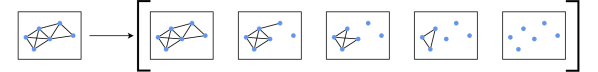
(a) A filtration sequence

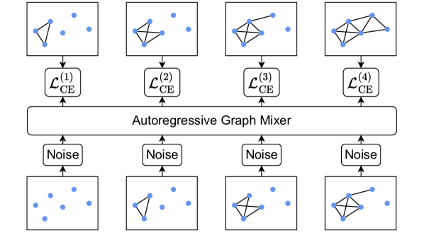
(b) Training stage I (teacher-forcing)

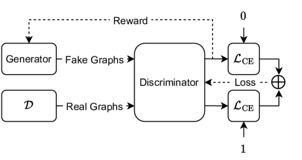
(c) Training stage II (adversarial fine-tuning)

Figure 1: Top: A graph is transformed into a sequence of subgraphs (filtration) via edge-deletion. Bottom left: the generator is trained via teacher-forcing to reverse the filtration process. Bottom right: the generator is fine-tuned in free-running mode via reinforcement learning on a reward signal output by a discriminator in a SeqGAN-like framework (c.f. Appendix K).

Filtrations from Node Orderings.

Many existing autoregressive models operate via node addition and thereby model sequences of nested induced subgraphs (You et al., 2018b; Li et al., 2018; Liao et al., 2019; Kong et al., 2023). We show that similar sequences may be obtained via filtration. In this sense, the filtration framework generalizes the sequences considered by these previous works. Given a graph $G$, let $g:V\to\{1,\dots,n\}$ be a node ordering, i.e., a bijection. Models that operate via node addition generate a graph sequence

$$(\emptyset,\emptyset)=G[V_{0}]\subseteq\dots\subseteq G[V_{T}]=G,$$ (3)

where $V_{0},\dots,V_{T}$ are monotonically increasing sub-levels of $g$ with $V_{t}=g^{-1}\left([(-\infty,a_{t}]\right)$ for some scalars $-\infty=a_{0}\leq\dots\leq a_{T}=+\infty$, and $G[V_{t}]$ denotes the induced subgraph whose node set is $V_{t}$. Now we consider the following filtration function $f:E\to\mathbb{R}$:

$$f(\{u,v\}):=\max\{g(u),g(v)\}\qquad\forall\{u,v\}\in E.$$ (4)

It is not hard to verify that this filtration function combined with the filtration schedule $\left(a_{t}\right)_{t=0}^{T}$, yields a filtration sequence $(G_{t})_{t=0}^{T}$ in which the edge set of $G_{t}$ coincides with the edge set of $G[V_{t}]$ for any $t=0,\dots,T$. Hence, this filtration closely mirrors the sequence of induced subgraphs, differing only in that the node set does not change over time. While a filtration function $f$ may be derived from any node ordering, we focus on depth-first search (DFS) orderings in this work, as shown to be optimal among several orderings for autoregressive graph generation in GRAN (Liao et al., 2019). For filtrations derived from DFS orderings, we choose the filtration schedule $a_{t}$ to linearly increase from a minimum edge weight at $t=1$ ($a_{1}=2$) to a maximum edge weight at $t=T$ ($a_{T}=|V|$). Unlike in previous autoregressive models (You et al., 2018b; Liao et al., 2019; Kong et al., 2023), $T$ is fixed across all graphs.

Line Fiedler Filtrations.

In contrast to the family of graph sequences leveraged by node-addition approaches, the filtration framework is not limited to sequences of induced subgraphs. We present the line Fiedler filtration function, which is one particular choice that, in general, yields a sequence of non-induced subgraphs. This function is derived from the second smallest eigenvector (Fiedler vector) of the symmetrically normalized Laplacian of the line graph $\mathrm{L}(G)$. In $\mathrm{L}(G)$, nodes represent edges in the original graph $G$, and two nodes are connected if their corresponding edges in $G$ share a common vertex. The line Fiedler filtration function captures global structural information and tends to assign similar values to neighboring edges. For $0\leq t\leq T$, we propose to define the filtration schedule $a_{t}$ as:

$$a_{t}:=\inf\left\{a\in\mathbb{R}\>:\>\frac{|f^{-1}((-\infty,a_{t}])|}{|E|}\geq\gamma(t/T)\right\},$$ (5)

where $f$ is the line Fielder filtration function, and $\gamma:[0,1]\to[0,1]$ is a monotonic function governing the rate at which edges are added in the filtration sequence. We choose $\gamma(t):=t$, leading to an approximately linear increase in the number of edges throughout the graph sequence. We investigate other choices of $\gamma$ in Appendix I.

4.2 Noise Augmentation of Filtrations

Our goal is to autoregressively generate sequences of graphs that approximately reverse the filtration processes above. To mitigate exposure bias in autoregressive modeling, previous works have proposed data augmentation schemes to make models more robust to the distribution shift occurring during inference (Bengio et al., 2015). We propose a simpler yet effective strategy: namely, randomly perturbing intermediate graphs in a filtration sequence $G_{0},\dots,G_{T}$ during the first training stage to expose the model to erroneous transitions. For each intermediate graph $G_{t}$ with $0<t<T$, we generate a perturbed graph $\tilde{G}_{t}$ with edge set $\tilde{E}_{t}$ by including each possible edge $e$ independently with probability

$$\mathbb{P}[e\in\tilde{E}_{t}]:=\left\{\begin{matrix}\begin{aligned} (1-\lambda_{t})+\lambda_{t}\rho_{t}&\quad\mathrm{if}\quad e\in E_{t}\\ \lambda_{t}\rho_{t}&\quad\mathrm{else}\end{aligned}\end{matrix}\right\},$$ (6)

where $\lambda_{t}\in[0,1]$ controls stochasticity and $\rho_{t}:=\nicefrac{{|E_{t}|}}{{\binom{|V|}{2}}}$ is the density of $G_{t}$. In practice, we decrease $\lambda_{t}$ linearly as $t$ increases and include multiple perturbations of each filtration sequence in the training set. The choice of hyper-parameters, such as $\lambda_{t}$ and the number of included perturbations, is detailed in Appendix E.2. We note that this augmentation yields possibly non-monotonic noisy filtration sequences $(\tilde{G_{t}})_{t=0}^{T}$ during training. Hence, our autoregressive model is trained to allow for edge deletions.

4.3 Autoregressive Modeling of Graph Sequences

The generative model will be trained to reverse the noise-augmented filtration process detailed above. We formulate the generative process using an autoregressive model, expressing the joint likelihood as follows:

$$p_{\theta}(\tilde{G}_{T},\dots,\tilde{G}_{0})=p(\tilde{G}_{0})\prod_{t=1}^{T}p_{\theta}(\tilde{G}_{t}|\tilde{G}_{t-1},\dots,\tilde{G}_{0}),$$ (7)

where $p(\tilde{G}_{0})$ represents the distribution over initial graphs, defined as a point mass on the fully disconnected graph $(V,\emptyset)$. In the following, we will detail our implementation of the autoregressive model $p_{\theta}$, including the architecture and training procedure. While existing autoregressive models typically utilize RNNs (You et al., 2018b; Liao et al., 2019; Goyal et al., 2020; Bacciu et al., 2020) or a first-order autoregressive structure (Kong et al., 2023), our model architecture for implementing $p_{\theta}$ is a novel and efficient design inspired by MLP-Mixers (Tolstikhin et al., 2021).

Backbone Architecture.

The graph sequences we consider can be viewed as dynamic graphs with constant node sets but evolving edge sets. Our backbone architecture operates on this structure by alternating between two types of information processing layers. The first type, called structural mixing, consists of a GNN that processes graph structures $\smash{\tilde{G}_{0},\makebox[8.00003pt][c]{.\hfil.\hfil.},\tilde{G}_{T-1}}$ independently, with weights shared across time steps. The second type, called temporal mixing, consists of a transformer decoder (TRDecoder) that processes node representations along the temporal axis, with weights shared across nodes. Our model inherits the causal structure of the transformer decoder, ensuring that node representations at timestep $t$ only depend on the graphs $\smash{\tilde{G}_{0},\makebox[8.00003pt][c]{.\hfil.\hfil.},\tilde{G}_{t}}$. Formally, given input node representations $\smash{v_{i}^{(t)}\in\mathbb{R}^{D}}$ for nodes $i\in V$ and time steps $t\in[T-1]$, a single mixing operation in our backbone model produces new representations $\smash{u_{i}^{(t)}}$ and is defined as:

$$\left(w_{i}^{(t)}\right)_{i=1}^{|V|} :=\operatorname{GNN}_{\theta}\left(\left(v_{i}^{(t)}\right)_{i=1}^{|V|},\,\tilde{E}_{t},\,t\right)\forall\>t=0,\makebox[7.20003pt][c]{.\hfil.\hfil.},T-1,$$

$$\left(u_{i}^{(t)}\right)_{t=1}^{T-1} :=\operatorname{TRDecoder}_{\theta}\left(\left(w_{i}^{(t)}\right)_{t=1}^{T-1}\right)\forall\>i=1,\makebox[7.20003pt][c]{.\hfil.\hfil.},|V|,$$

where the first equation defines a structural mixing operation and the second equation defines a temporal mixing operation. For the structural mixing, we use Structure-Aware-Transformer layers (Chen et al., 2022). Additionally, we incorporate both the timestep $t$ and cycle counts in $\tilde{G}_{t}$ using FiLM (Perez et al., 2018). These structural features were used previously in other graph generative models such as DiGress (Vignac et al., 2023). Multiple mixing operations are stacked to form the backbone model.

Edge Decoder.

To model $p_{\theta}(\tilde{G}_{t}|\tilde{G}_{t-1},\dots,\tilde{G}_{0})$, we produce a distribution over possible edge sets of $\tilde{G}_{t}$. We use a mixture of multivariate Bernoulli distributions to capture dependencies between edges, similar to previous works (Liao et al., 2019; Kong et al., 2023). Given $K\geq 1$ mixture components, we infer $K$ Bernoulli parameters for each node pair $i,j\in V$ from the node representations $v_{i}$ produced by the backbone model at timestep $t-1$:

$$p_{k}^{(i,j)}:=D_{k,\theta}(v_{i},v_{j})\in[0,1],$$ (8)

where $k=1,\makebox[8.00003pt][c]{.\hfil.\hfil.},K$ and $D_{\cdot,\theta}$ is some neural network. We enforce that $\smash{p_{k}^{(i,j)}}$ is symmetric and that the probability of self-loops is zero. In addition, we produce a mixture distribution $\pi\in\mathbb{R}^{K}$ in the $K-1$ dimensional probability simplex from pooled node representations. The architectural details of $D_{\cdot,\theta}$ are provided in Appendix F.2. The final likelihood is defined as:

$$\small p_{\theta}(\tilde{E}_{t}|\tilde{G}_{t-1},\makebox[7.20003pt][c]{.\hfil.\hfil.},\tilde{G}_{0}):=\sum_{k=1}^{K}\pi_{k}\prod_{i<j}\left\{\begin{matrix}\begin{aligned} p_{k}^{(i,j)}&\;\mathrm{if}\;e_{ij}\in\tilde{E}_{t}\\ 1-p_{k}^{(i,j)}&\;\mathrm{else}\end{aligned}\end{matrix}\right\}\normalsize$$

In contrast to existing autoregressive graph generators (You et al., 2018b; Liao et al., 2019; Goyal et al., 2020; Bacciu et al., 2020; Kong et al., 2023), our model introduces a key innovation: the ability to generate non-monotonic graph sequences. This means it can both add and delete edges. We argue that this capability is crucial for mitigating error accumulation during sampling (i.e., exposure bias). Consider, for instance, the task of generating tree structures. If a cycle is inadvertently introduced into an intermediate graph $\tilde{G}_{t}$ (where $t<T$), traditional autoregressive approaches would be unable to rectify this error. Our model, however, can potentially delete the appropriate edges in subsequent timesteps, thus recovering from such mistakes. The noise augmentation approach from Sec. 4.2 exposes ANFM to such erroneous transitions during training. We show empirically in Sec. 5.4 that this augmentation substantially improves performance.

Input Node Representations.

The initialization of node representations is a crucial step preceding the forward pass through the mixer architecture above. We compute initial node representations from positional and structural features in a similar fashion as Vignac et al. (2023). Moreover, we add learned positional embeddings based on a node ordering derived from the filtration function. We refer to Appendix F.1 for further details.

Asymptotic Complexity.

We provide a detailed analysis of the asymptotic runtime complexity of our method in Appendix C.1. Asymptotically, ANFM’s complexity of sampling a graph with $N$ nodes is $\mathcal{O}(T^{2}N+TN^{3})$, where we recall that $T$ denotes the number of filtration steps. Although cubic in the number of nodes, we found that the efficiency of ANFM is largely driven by our ability to use a small $T$ ($T\leq 32$), while diffusion-based models generally require a much larger number of iterations.

4.4 Training Algorithm

Teacher-Forcing.

We employ teacher-forcing (Williams & Zipser, 1989) to train our generative model $p_{\theta}$ in a first training stage. We illustrate this training scheme in Figure 1(b). Teacher-forcing allows the model to learn from complete sequences of graph evolution, providing a good initialization for subsequent reinforcement learning-based fine-tuning. Given a dataset of graphs $\mathcal{D}$, we convert it into a dataset of noisy filtration sequences, denoted as $\tilde{\mathcal{D}}$. Our objective is to maximize the log-likelihood of these sequences under our model:

$$\mathcal{L}(\theta):=\mathbb{E}_{(\tilde{G}_{0},\dots,\tilde{G}_{T})\sim\tilde{\mathcal{D}}}\left[\log p_{\theta}(\tilde{G}_{0},\dots,\tilde{G}_{T})\right].$$ (9)

In practice, this objective is implemented as a cross-entropy loss. While the noise augmentation introduced in Sec. 4.2 improves the overall quality of generated graphs after teacher-forcing training, it still falls short in generating graphs with high structural validity. To further mitigate exposure bias, we propose an RL-based fine-tuning stage to refine the model trained with teacher-forcing.

Adversarial Fine-tuning with RL.

Adapting the SeqGAN framework (Yu et al., 2017), we implement a generator-discriminator architecture where the generator (our mixer model) operates in inference mode as a stochastic policy and is thereby exposed to its own predictions during training. The discriminator is a graph transformer, namely GraphGPS (Rampásek et al., 2022). During training, the generator produces graph samples, which the discriminator evaluates for plausibility. The generator is updated using Proximal Policy Optimization (PPO) (Schulman et al., 2017) based on the discriminator’s feedback, while the discriminator is trained adversarially to distinguish between generated and training set graphs. This training scheme is illustrated in Figure 1(c). It is worth noting that only the final generated graph is presented to the discriminator. Therefore, the generator is trained to maximize a terminal reward without constraints on intermediate graphs. We provide pseudo-code in Appendix K.

5 Experiments

We empirically evaluate our method on synthetic and real-world datasets. We investigate the filtration strategy based on depth-first search node orderings (DFS) and the line Fiedler function (Fdl.). In Sec. 5.1, we first present results on the commonly used small benchmark datasets (Martinkus et al., 2022), comparing our method to a variety of baselines. We then demonstrate in Sec. 5.2 that we can improve upon these results by using a more realistic setting with more training examples. Additionally, we present results for inference efficiency. Finally, in Sec. 5.3, we demonstrate that our model is applicable to real-world data, namely larger protein graphs (Dobson & Doig, 2003) and drug-like molecules (Brown et al., 2019). In Sec. 5.4, we present ablation studies demonstrating the efficacy of noise augmentation and adversarial fine-tuning.

Evaluation.

We follow established practices from previous works (You et al., 2018b; Martinkus et al., 2022; Vignac et al., 2023) in our evaluation. We compare a set of model-generated samples to a test set via maximum mean discrepancy (MMD) (Gretton et al., 2012), based on various graph descriptors. These descriptors include histograms of node degrees (Deg.), clustering coefficients (Clus.), orbit count statistics (Orbit), and eigenvalues (Spec.).

In previous works (Martinkus et al., 2022; Vignac et al., 2023), very few samples are generated for the evaluation of graph generative models. In Appendix J, we show theoretically and empirically that this leads to high bias and variance in the reported metrics. In Sec. 5.2 and 5.3, we generate 1024 samples for evaluation to mitigate this, while we generate 40 samples in Sec. 5.1 to fairly compare to previous methods. For synthetic datasets, we follow previous works by reporting the ratio of generated samples that are valid, unique, and novel (VUN). In Sec. 5.2 and 5.3, we report inference speed, measured as the time needed to generate 1024 graphs on an H100 GPU, normalized to a per-graph cost.

Baselines.

We aim to demonstrate that our method is competitive with state-of-the-art diffusion models in terms of sample quality while outperforming them in terms of inference speed. Hence, we compare our method to two recent diffusion models, namely DiGress (Vignac et al., 2023) and ESGG (Bergmeister et al., 2024). DiGress first introduced discrete diffusion to the area of graph generation and remains one of the most robust baselines. ESGG is acutely relevant to our work, as it aims to improve inference speed. In addition, we also present results on an autoregressive model, GRAN (Liao et al., 2019), which focuses on efficiency during inference. For details on model selection and hyper-parameters for these baselines, we refer to Sections H.5, H.1, H.2, H.3 and H.4. In Sec. 5.1, we report baseline results from the literature, also comparing to the hierarchical HiGen (Karami, 2024) approach, the scalable EDGE (Chen et al., 2023) diffusion model, the autoregressive GraphRNN model (You et al., 2018b), and the GAN-based SPECTRE model (Martinkus et al., 2022).

5.1 Experiments with Small Synthetic Datasets

Table 1: Performance of models on small synthetic SPECTRE datasets. Results on GraphRNN, GRAN and SPECTRE taken from Martinkus et al. (2022). Results on DiGress, ESGG and EDGE from Bergmeister et al. (2024).

	Planar Graphs ($|V|=64$, $N_{\mathrm{train}}=128$)
	VUN ($\uparrow$)	Deg. ($\downarrow$)	Clus. ($\downarrow$)	Orbit ($\downarrow$)	Spec. ($\downarrow$)
GraphRNN	$0.0$	$0.0049$	$0.2779$	$1.2543$	$0.0459$
GRAN	$0.0$	$0.0007$	$0.0426$	$0.0009$	$0.0075$
SPECTRE	$25.0$	$0.0005$	$0.0785$	$0.0012$	$0.0112$
DiGress	$77.5$	$0.0007$	$0.0780$	$0.0079$	$0.0098$
EDGE	$0.0$	$0.0761$	$0.3229$	$0.7737$	$0.0957$
ESGG	$95.0$	$0.0005$	$0.0626$	$0.0017$	$0.0075$
ANFM (Fdl.)	$72.5$	$0.0037$	$0.1332$	$0.0047$	$0.0099$
ANFM (DFS)	$37.5$	$0.000\,350\,088\,024\,399\,841\,66$	$0.030\,911\,077\,240\,092\,955$	$0.001\,170\,927\,314\,442\,016\,3$	$0.006\,111\,137\,605\,895\,989$

	SBM Graphs ($|V|\sim 104$, $N_{\mathrm{train}}=128$)
	VUN ($\uparrow$)	Deg. ($\downarrow$)	Clus. ($\downarrow$)	Orbit ($\downarrow$)	Spec. ($\downarrow$)
GraphRNN	$5.0$	$0.0055$	$0.0584$	$0.0785$	$0.0065$
GRAN	$25.0$	$0.0113$	$0.0553$	$0.0540$	$0.0054$
SPECTRE	$52.5$	$0.0015$	$0.0521$	$0.0412$	$0.0056$
DiGress	$60.0$	$0.0018$	$0.0485$	$0.0415$	$0.0045$
EDGE	$0.0$	$0.0279$	$0.1113$	$0.0854$	$0.0251$
HiGen	N/A	0.0019	0.0498	0.0352	0.0046
ESGG	$45.0$	$0.0119$	$0.0517$	$0.0669$	$0.0067$
ANFM (Fdl.)	$47.5$	$0.0014$	$0.0506$	$0.0551$	$0.0058$
ANFM (DFS)	$65.0$	$0.000\,650\,452\,916\,583\,388\,3$	$0.048\,835\,624\,180\,876\,655$	$0.033\,512\,100\,695\,272\,66$	$0.004\,814\,343\,171\,210\,655\,5$

As a first demonstration of our method, we present results on the planar and SBM datasets by Martinkus et al. (2022). Since the training set consists of only 128 graphs, we find that ANFM models using the line Fiedler function tend to overfit during the teacher-forcing training stage. To mitigate this issue, we introduce some small stochastic perturbations to node orderings used for initializing node representations. We discuss this in more detail in Appendix F.1. Model selection is performed based on the minimal validation loss. Table 1 illustrates that, in terms of VUN on the planar graph dataset, our models outperform GraphRNN (You et al., 2018b), GRAN (Liao et al., 2019), EDGE (Chen et al., 2023), and SPECTRE (Martinkus et al., 2022). They perform slightly worse than DiGress (Vignac et al., 2023) and ESGG (Bergmeister et al., 2024). While the line Fiedler variant outperforms the DFS variant on the planar graph dataset, the DFS variant performs substantially better on the SBM dataset. Notably on the SBM dataset, the DFS variant outperforms all baselines w.r.t. VUN and most MMD metrics. On both datasets, ANFM is competitive with the two diffusion-based approaches, DiGress and ESGG.

5.2 Experiments with Expanded Synthetic Datasets

Table 2: Performance on expanded synthetic datasets, evaluated on 1024 model samples. Showing a single run for the baselines and DFS, the median across three runs for the line Fiedler variant. *ESGG evaluation modified to draw graph sizes from empirical training distribution and use 100 refinement steps for determining SBM validity.

	Expanded Planar Graphs ($|V|=64$, $N_{\mathrm{train}}=8192$)
	VUN ($\uparrow$)	Deg. ($\downarrow$)	Clus. ($\downarrow$)	Orbit ($\downarrow$)	Spec. ($\downarrow$)	Time ($\downarrow$)
GRAN	$0.192\,31$	$0.006\,113\,867\,711\,138\,976$	$0.186\,243\,286\,394\,872\,48$	$0.096\,055\,223\,126\,866\,76$	$0.008\,104\,395\,492\,142\,48$	$0.030\,334\,320\,85$
DiGress	$80.761\,72$	$0.000\,416\,493\,119\,631\,988\,8$	$0.021\,730\,750\,835\,276\,424$	$0.004\,488\,442\,523\,941\,76$	$0.002\,425\,416\,821\,497\,883\,3$	$2.726\,342\,486\,68$
ESGG*	$89.941\,41$	$0.000\,726\,508\,788\,436\,497\,4$	$0.016\,175\,366\,554\,288\,972$	$0.007\,441\,655\,511\,178\,702$	$0.001\,232\,535\,862\,508\,266$	$4.649\,525\,286\,86$
ANFM (Fdl.)	$79.199\,22$	$0.000\,383\,280\,816\,482\,312\,05$	$0.018\,315\,733\,274\,652\,524$	$0.000\,188\,098\,802\,662\,350\,9$	$0.001\,198\,020\,860\,018\,855\,8$	$0.015\,363\,676\,93$
ANFM (DFS)	$45.605\,47$	$0.000\,312\,928\,398\,365\,608\,4$	$0.029\,550\,210\,939\,678\,245$	$0.000\,444\,722\,907\,314\,787\,36$	$0.001\,685\,905\,166\,112\,666\,7$	$0.016\,376\,615\,96$

	Expanded SBM Graphs ($N_{\mathrm{train}}=8192$)
	VUN ($\uparrow$)	Deg. ($\downarrow$)	Clus. ($\downarrow$)	Orbit ($\downarrow$)	Spec. ($\downarrow$)	Time ($\downarrow$)
GRAN	$25.288\,46$	$0.018\,554\,194\,034\,812\,62$	$0.008\,552\,612\,861\,186\,321$	$0.030\,485\,389\,289\,185\,87$	$0.002\,193\,005\,558\,297\,933\,5$	$0.132\,553\,174\,16$
DiGress	$56.152\,34$	$0.000\,187\,617\,138\,546\,425\,37$	$0.005\,575\,554\,031\,473\,584$	$0.007\,552\,669\,961\,076\,439$	$0.000\,948\,721\,322\,645\,784\,8$	12.99
ESGG*	$3.515\,62$	$0.094\,870\,369\,415\,710\,92$	$0.012\,106\,638\,671\,567\,905$	$0.051\,814\,069\,099\,514\,86$	$0.012\,239\,075\,476\,934\,591$	$39.417\,137\,279\,9$
ANFM (Fdl.)	$75.976\,56$	$0.001\,438\,607\,730\,545\,049\,5$	$0.005\,062\,382\,182\,491\,599$	$0.018\,009\,643\,354\,469\,057$	$0.001\,141\,348\,405\,031\,772\,4$	$0.039\,569\,466\,6$
ANFM (DFS)	$78.027\,34$	$0.000\,794\,559\,290\,614\,893\,5$	$0.004\,853\,086\,793\,020\,355\,5$	$0.004\,919\,597\,001\,513\,051$	$0.000\,813\,837\,757\,143\,165\,4$	$0.039\,739\,082\,33$

	Expanded Lobster Graphs ($N_{\mathrm{train}}=8192$)
	VUN ($\uparrow$)	Deg. ($\downarrow$)	Clus. ($\downarrow$)	Orbit ($\downarrow$)	Spec. ($\downarrow$)	Time ($\downarrow$)
GRAN	$41.992\,19$	$0.043\,648\,945\,494\,517\,48$	$0.006\,875\,850\,695\,025\,276$	$0.150\,963\,183\,136\,294\,3$	$0.146\,936\,353\,003\,071\,4$	$0.039\,924\,433\,22$
DiGress	$96.582\,03$	$0.000\,097\,928\,492\,235\,110\,92$	$0.000\,000\,832\,987\,332\,000\,1$	$0.001\,584\,719\,768\,310\,094\,4$	$0.000\,911\,882\,425\,339\,349\,8$	$4.859\,872\,366\,07$
ESGG*	$63.964\,84$	$0.000\,676\,779\,484\,502\,176\,8$	$0$	$0.002\,662\,508\,131\,173\,302\,3$	$0.002\,318\,797\,647\,705\,928$	$3.156\,260\,820\,11$
ANFM (Fdl.)	$79.101\,56$	$0.000\,403\,299\,865\,038\,953$	$7.888\,505\,157\,871\,428\text{\times}{10}^{-05}$	$0.001\,043\,212\,982\,421\,16$	$0.001\,578\,534\,329\,912\,617\,6$	$0.017\,485\,590\,18$
ANFM (DFS)	$87.597\,66$	$7.824\,159\,351\,721\,427\text{\times}{10}^{-05}$	$1.641\,427\,338\,494\,594\,3\text{\times}{10}^{-06}$	$0.000\,727\,856\,308\,562\,202\,5$	$0.000\,967\,362\,477\,460\,209\,6$	$0.015\,996\,707\,83$

We supplement the results presented above by training our model on larger synthetic datasets. Namely, we generate training sets consisting of $8192$ graphs and corresponding validation and test sets consisting of 256 graphs each. We use the same data generation approach as in Martinkus et al. (2022) to obtain expanded planar and SBM datasets. Additionally, we produce an expanded dataset of lobster graphs using NetworkX (Hagberg et al., 2008), as done in (Liao et al., 2019). We perform one training run per dataset for the DFS variant and three independent runs for the line Fiedler variant to illustrate robustness. We present the deviations observed across the three runs in Appendix G.1 and visualize samples from our model in Appendix G.2. In Table 2, we compare our method to our three baselines. For reasons of brevity, we only report the median performance here. All models reach perfect uniqueness and novelty scores on the expanded planar and SBM datasets and comparable uniqueness and novelty performance on the expanded lobster dataset (c.f. Appendix G.1). We find that ANFM is substantially faster during inference than the diffusion models, consistently achieving at least a 100-fold speedup in comparison to DiGress and ESGG. Moreover, we find that our method appears competitive with respect to sample quality, outperforming the two diffusion models on the expanded SBM dataset in terms of validity. For ESGG, we note that we obtain a surprisingly low validity score on the expanded SBM dataset and refer to Appendix H.5 for further discussion on this. We find that ANFM substantially outperforms the autoregressive baseline, GRAN, in terms of validity and MMD metrics.

5.3 Experiments with Real-World Data

In this subsection, we present empirical results on the protein graph dataset introduced by Dobson & Doig (2003) and the GuacaMol (Brown et al., 2019) dataset consisting of drug-like molecules.

Proteins.

While results have been reported for the protein dataset in previous works, we re-evaluate the baselines on 1024 model samples to reduce bias and variance in the reported metrics. We use a trained GRAN checkpoint provided by Liao et al. (2019) but re-train ESGG and DiGress, as no trained models are available.

Table 3: Performance of models on protein graph dataset. *Graph sizes are drawn from empirical training distribution.

	Protein Graphs ($100\leq|V|\leq 500$, $N_{\mathrm{train}}=587$)
	Deg. ($\downarrow$)	Clus. ($\downarrow$)	Orbit ($\downarrow$)	Spec. ($\downarrow$)	Time ($\downarrow$)
GRAN	$0.002\,529\,266\,715\,085\,798\,4$	$0.050\,974\,335\,560\,261\,84$	$0.153\,874\,257\,369\,359\,45$	$0.005\,050\,147\,221\,974\,61$	2.25
DiGress	$0.000\,560\,570\,322\,663\,211\,9$	$0.023\,397\,315\,700\,488\,697$	$0.028\,867\,965\,119\,309\,78$	$0.001\,421\,093\,317\,606\,425\,5$	$72.274\,187\,582\,5$
ESGG*	$0.003\,271\,463\,212\,130\,454\,3$	$0.021\,593\,122\,621\,891\,67$	$0.055\,739\,136\,119\,765\,44$	$0.000\,811\,374\,942\,401\,466$	$19.478\,365\,687\,2$
ANFM (Fdl.)	$0.002\,374\,902\,505\,834\,830\,5$	$0.046\,388\,453\,880\,653\,09$	$0.053\,196\,405\,429\,128\,07$	$0.002\,364\,090\,587\,438\,25$	$0.194\,417\,011\,92$
ANFM (DFS)	$0.002\,433\,803\,382\,213\,550\,7$	$0.037\,010\,678\,780\,236\,66$	$0.062\,028\,807\,744\,423\,764$	$0.001\,997\,214\,985\,000\,051$	$0.190\,862\,149\,23$

We find that our model is again substantially faster than the diffusion-based baselines. Moreover, it is also 10 times faster than GRAN while outperforming it with respect to all MMD metrics. In comparison to the diffusion-based models, the sample quality of our approach appears slightly worse by most MMD metrics.

GuacaMol.

So far, we have focused on generating un-attributed graphs. However, molecular structures require node and edge labels to represent atom and bond types, respectively. Inspired by the approach of Li et al. (2020), we first train ANFM to generate un-attributed topologies and then assign node and edge labels using a simple VAE. Details of this post-hoc labeling procedure can be found in Appendix B. In Table 4, we compare the performance of ANFM to several baselines from Vignac et al. (2023), namely an LSTM model trained on SMILES strings (Brown et al., 2019), graph MCTS (Brown et al., 2019), and NAGVAE (Kwon et al., 2020). Notably, ANFM demonstrates competitive performance with DiGress.

Table 4: Performance of models on GuacaMol benchmark.

	GuacaMol ($2\leq|V|\leq 88$, $N_{\mathrm{train}}\approx 1.3M$)
	Valid ($\uparrow$)	Unique ($\uparrow$)	Novel ($\uparrow$)	KL Div ($\uparrow$)	FCD ($\uparrow$)
LSTM	95.9	100	91.2	99.1	91.3
NAGVAE	92.7	95.5	100	38.4	0.9
MCTS	100	100	99.4	52.2	1.5
DiGress	85.2	100	99.9	92.9	68.0
ANFM (DFS)	$75.64$	$99.99$	$98.31$	$95.051\,757\,853\,025\,68$	$65.200\,212\,551\,745\,84$

5.4 Ablation Studies

In this subsection, we demonstrate that noise augmentation and adversarial fine-tuning are crucial components of our method. We interpret this as a strong indication that exposure bias affects our autoregressive model. Additionally, we study the impact of the filtration granularity, as determined by the hyper-parameter $T$. In Appendix I, we present extensive additional ablations.

Table 5: Two ablation studies using the line Fiedler variant on the expanded planar graph dataset. Showing median $\pm$ maximum deviation across three runs. For the noise ablation, we train for 100k steps in stage I. For the finetuning ablation, we train for 200k steps in stage I.

	Noise Ablation		Finetuning Ablation
	Stage I w/ Noise	Stage I w/o Noise	Stage II	Stage I w/ Noise
VUN ($\uparrow$)	$20.214\,84$ $\pm$ $3.222\,66$	$0.0$ $\pm$ $0.0$	$79.199\,22$ $\pm$ $7.128\,91$	$23.242\,19$ $\pm$ $9.667\,97$
Deg. ($\downarrow$)	$0.005\,753\,176\,855\,113\,784$ $\pm$ $0.000\,841\,566\,690\,248\,152\,2$	$0.086\,418\,290\,533\,905\,04$ $\pm$ $0.074\,923\,072\,401\,962\,94$	$0.000\,383\,280\,816\,482\,312\,05$ $\pm$ $5.425\,587\,654\,261\,932\text{\times}{10}^{-05}$	$0.003\,582\,931\,553\,877\,344\,3$ $\pm$ $0.000\,873\,549\,111\,093\,829\,8$
Clus. ($\downarrow$)	$0.176\,845\,325\,553\,082$ $\pm$ $0.010\,596\,256\,629\,278\,128$	$0.317\,862\,805\,092\,968\,44$ $\pm$ $0.003\,679\,679\,225\,341\,181\,4$	$0.018\,315\,733\,274\,652\,524$ $\pm$ $0.001\,394\,485\,118\,883\,626$	$0.154\,693\,717\,870\,596\,83$ $\pm$ $0.027\,969\,526\,095\,574\,127$
Spec. ($\downarrow$)	$0.004\,760\,004\,557\,846\,642$ $\pm$ $0.001\,062\,101\,856\,279\,307\,2$	$0.104\,154\,601\,460\,458\,41$ $\pm$ $0.075\,992\,169\,630\,051\,4$	$0.001\,198\,020\,860\,018\,855\,8$ $\pm$ $0.000\,402\,135\,017\,207\,427\,84$	$0.003\,302\,054\,948\,134\,847$ $\pm$ $0.001\,386\,189\,236\,599\,833$
Orbit ($\downarrow$)	$0.012\,890\,572\,283\,490\,664$ $\pm$ $0.016\,881\,716\,403\,595\,26$	$0.711\,463\,963\,920\,079\,6$ $\pm$ $0.441\,082\,020\,882\,348\,6$	$0.000\,188\,098\,802\,662\,350\,9$ $\pm$ $0.001\,574\,797\,976\,899\,633\,4$	$0.004\,284\,029\,842\,958\,059$ $\pm$ $0.002\,323\,286\,420\,590\,653\,4$

Noise Augmentation.

We find that noise augmentation of intermediate graphs substantially improves performance during training with teacher forcing (stage I). We illustrate this using the line Fiedler variant on the expanded planar graph dataset in Table 5. A corresponding experiment for the DFS variant can be found in Appendix I.

GAN Tuning.

In Table 5, we compare performance after training with teacher-forcing and subsequent adversarial fine-tuning on the expanded planar graph dataset. We find that adversarial fine-tuning substantially improves performance, both in terms of validity and MMD metrics. A corresponding analysis for the DFS variant and the expanded SBM and lobster datasets can be found in Appendix I.

Filtration Granularity.

In Figure 2, we study the impact of filtration granularity, i.e., the number of steps $T$, on generation quality and speed of ANFM. Analogously, we investigate how the number of denoising steps influences quality and speed in DiGress. We re-train the models with varying $T$. ANFM consistently outperforms DiGress in computational efficiency across all $T$. While DiGress only achieves a maximum VUN of 41% for our largest considered $T$, ANFM achieves a VUN of 81% for $T=30$.

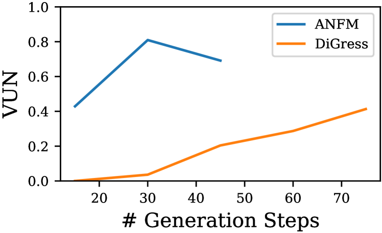
(a) Planar VUN vs $T$

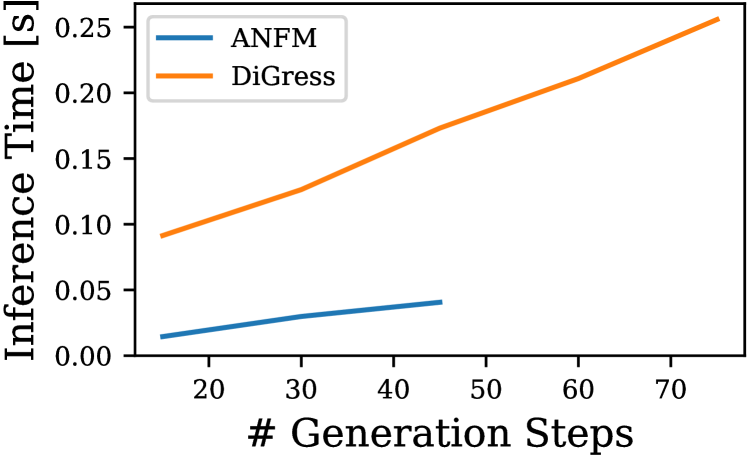
(b) Inference time vs $T$

Figure 2: Performance of ANFM and DiGress on the expanded planar dataset as number of generation steps varies.

6 Conclusion

We proposed ANFM, an efficient autoregressive graph generative model that relies on graph filtration. The filtration framework generalizes previous autoregressive approaches that operate via node addition, providing additional flexibilities in the choice of graph sequences. ANFM generates high-quality graphs, outperforming existing autoregressive models and rivaling discrete diffusion approaches in terms of quality while being substantially faster at inference. Various ablations demonstrated the configurability of ANFM and indicated that exposure bias is an important challenge for autoregressive graph modeling.

While we have demonstrated that attributes may be sampled in a post-hoc fashion using a VAE, direct modeling within ANFM remains an interesting area for future investigation. We also highlight issues with existing benchmark datasets, where small sample sizes during evaluation lead to unreliable results with high variance and bias. Systematically addressing these challenges is essential for enabling more reliable and fair benchmarking in future research.

Impact Statement

We have introduced ANFM, a method for high-throughput graph generation. There are many well-established societal implications of advancing the field of machine learning in general, which also apply to our work. The use of graph generative models in drug discovery represents one particularly impactful application with potentially significant benefits for public health. As these advancements shape the future of medicine, it is crucial to promote their responsible use and ensure that their benefits remain widely accessible.

Appendix

This appendix is organized as follows: We discuss additional related work in Appendix A and provide details on post-hoc attribute generation in Appendix B. In Appendix C, we analyze the runtime complexity of ANFM and investigate a variant that is asymptotically more efficient w.r.t. $T$. In Appendix D, we show that we optimize a lower-bound on the data log-likelihood in training stage I. Details on hyperparameters and model architecture are provided in Appendices E and F. We provide evaluation results across several runs and qualitative model samples in Appendix G. Appendix H provides details on our baselines. Additional ablations on filtration function, schedule, node individualization, etc., are presented in Appendix I. We discuss the shortcomings of established evaluation approaches in Appendix J. Finally, we detail the adversarial finetuning algorithm in Appendix K.

Appendix A Extended Related Work

In this section, we extend Sec. 2 and provide additional comparative analyses to previous works.

Other Graph Generative Models.

In concurrent work, Zhao et al. (2024) introduce a hybrid graph generative model, termed Pard, combining autoregressive and discrete diffusion components. Similar to ANFM, Pard generates graphs by building a sequence of increasingly large subgraphs. In contrast to the method we present here, Pard is limited to the generation of induced subgraphs and uses a shared diffusion model to sample them. While the authors state efficiency as one motivation for their approach, they do not present runtime measurements during inference.

Graph Denoising Diffusion.

Similar to graph denoising diffusion models (Vignac et al., 2023), we propose a corrupting process to transform graph samples $G_{T}$ into graphs $G_{0}$ from some convergent distribution (in our case the point-mass at the completely disconnected graph). However, in contrast to denoising diffusion models, the process we are proposing is not Markov.

Absorbing State Diffusion.

Absorbing state graph diffusion (Chen et al., 2023; Kong et al., 2023) resembles our approach in that it also generates a sequence of increasingly dense graphs. We aim to increase efficiency by generating substantially shorter sequences than previous works. In practice, we choose to generate graphs within 15 or 30 steps. EDGE (Chen et al., 2023) requires between 64 and 512 denoising steps, depending on the dataset. To generate a graph on $N$ nodes, GraphARM (Kong et al., 2023) requires $N$ denoising steps, as exactly one node decays to the absorbing state at a time. The larger number of denoising steps in these methods may increase inference time and necessitates a first-order autoregressive structure. Additionally, as detailed above, our proposed method does not readily fit into the framework of denoising diffusion models. Moreover, ANFM may generate non-monotonic graph sequences.

RL in Graph Generation.

In the context of graph generation, reinforcement learning has been mostly used for molecular graphs.  You et al. (2018a) train a generative model for molecules via reinforcement learning, combining adversarial and domain-specific rewards. In contrast to our work, they only consider molecular graphs and do not use teacher-forcing for training. Taiga (Mazuz et al., 2023) uses reinforcement learning to optimize the chemical properties of molecules obtained from a language model pre-trained on SMILES strings. Diffusion models have also been shown to be amenable to RL finetuning, allowing extrinsic non-differentiable metrics to be optimized (Liu et al., 2024).

Appendix B Generating Attributed Graphs

B.1 Variational Inference

To generate attributed graphs $(G,l_{V},l_{E})$ with topology $G$ and node and edge labels $l_{V}$ and $l_{E}$, we propose to first generate the un-attributed graph topology using ANFM. Subsequently, we label nodes and edges using a separate model. I.e., we decompose the joint distribution as:

$$p_{\theta}(G,l_{V},l_{E})=p_{\theta}^{\mathrm{label}}(l_{E},l_{V}\>|\>G)\cdot p_{\theta}^{\mathrm{ANFM}}(G)$$ (10)

where $p_{\theta}^{\mathrm{label}}$ generates node and edge attributes. We take inspiration from Li et al. (2020) and train $p_{\theta}^{\mathrm{label}}$ as a variational autoencoder.

Variational Inference.

Let $G:=(V,E)$ be a graph topology from the training dataset and let $l_{V}:V\to\mathcal{X}$ and $l_{E}:E\to\mathcal{Y}$ be ground-truth node and edge labels for $G$, respectively. An encoder $q_{\phi}$ maps the labeled graph $(G,l_{V},l_{E})$ to a distribution over $D$-dimensional latent node representations $\bm{z}\in\mathbb{R}^{V\times D}$. A decoder $p_{\theta}$ maps a tuple $(G,\bm{z})$, i.e. the graph topology combined with a latent representation, to a distribution over node and edge attributes. In practice, we consider discrete attributes and $p_{\theta}$ parametrizes a product distribution across nodes and edges. If $\mathcal{X}$ or $\mathcal{Y}$ factorize into a product of simpler spaces (i.e., when there are multiple node or edge attributes), $p_{\theta}$ parametrizes a corresponding product distribution over $\mathcal{X}$ or $\mathcal{Y}$. The encoder $q_{\phi}$ parametrizes a Gaussian distribution with a diagonal covariance matrix. We formulate the typical evidence lower bound (Kingma & Welling, 2014):

$$p_{\theta}(l_{E},l_{V}\>|\>G)\geq\mathbb{E}_{\bm{z}\sim q_{\phi}(\>\cdot\>|\>G,l_{E},l_{V})}\left[p_{\theta}(l_{E},l_{V}\>|\>G,\bm{z})\right]-D_{\mathrm{KL}}\left(q_{\phi}(\>\cdot\>|\>G,l_{E},l_{V})\>|\>\mathcal{N}(\bm{0},I)\right)$$ (11)

Architecture.

We implement $q_{\phi}$ and $p_{\theta}$ as GraphGPS (Rampásek et al., 2022) models. Since $q_{\phi}$ operates on edge-labeled graphs, we use GINE message passing layers (Hu et al., 2020) within its graph transformer. The decoder $p_{\theta}$, on the other hand, only operates on node representations, and we therefore use GIN layers (Xu et al., 2019). The two GNNs are provided with Laplacian and random walk positional embeddings (Dwivedi et al., 2022) and we use 5% dropout layers (Srivastava et al., 2014). We feed the node representations produced by $p_{\theta}$ through MLPs to generate distributions over node attributes. To generate a distribution over the attribute of an edge $\{u,v\}$, we add the node representations corresponding to $u$ and $v$ and feed the resulting vector through an MLP.

Training.

We train $q_{\phi}$ and $p_{\theta}$ jointly by maximizing a re-weighted version of the ELBO in Eqn. (11). Specifically, we divide the loss for a given datum $(G,l_{E},l_{V})$ by $|V|$, the cardinality of the node set of $G$.

Sampling.

To sample attributes, we draw latent node representations $\bm{z}$ from the standard normal distribution. We select the maximum likelihood node and edge attributes from $p_{\theta}(\>\cdot\>|\>G,\bm{z})$. The encoder $q_{\phi}$ may be discarded after training.

B.2 Details on GuacaMol Experiments

Below, we provide details on the molecule graph generation presented in Sec. 5.3. As described in Appendix B, we train ANFM on the un-attributed molecule topologies of GuacaMol. Independently, we train a VAE to generate attributes conditioned on a topology. To sample a molecule, we first generate a graph using ANFM and label nodes and edges using the VAE.

Attributes.

We produce edge labels that indicate the bond type between heavy atoms, distinguishing between single, double, triple, and aromatic bonds. To reconstruct the correct molecule from its graph representation, we find that we require require several node attributes. Namely, given an atom (i.e., node), we generate its type (i.e., the element), the number of explicit hydrogens bound to it, the number of radical electrons, and its partial charge.

ANFM Hyperparameters.

We train an ANFM model using the DFS filtration strategy. In stage I, we use similar hyper-parameters as for the other datasets. We use $T=30$ filtration steps, a learning rate of $10^{-5}$, a local batch size of 64 on two GPUs, and 300k training steps. Throughout stage I training, we monitor validation loss and ensure that the model does not overfit. During training stage II, we use a batch size of 32 and a learning rate of $2.5\times 10^{-8}$ for the generative model. The discriminator has 3 layers and a hidden dimension of 32. The other hyperparameters of the discriminator and value model match those used in the other experiments.

VAE Hyperparameters.

We use 5-layer GraphGPS (Rampásek et al., 2022) models for the encoder and decoder, respectively. The hidden dimension is 256 while we choose the latent dimension $D$ to be 8. The Laplacian positional embedding is 3-dimensional while the random walk positional embedding is 8-dimensional. We train for 250 epochs on the GuacaMol dataset, using a batch size of 512, an Adam optimizer (Kingma & Ba, 2015) and a learning rate of $10^{-4}$.

Model Samples.

In Figure 3, we show uncurated samples from the ANFM model.

Figure 3: Uncurated samples from ANFM model trained on GuacaMol.

Appendix C Sampling Complexity of ANFM

C.1 Complexity Analysis

In the following, we analyze the asymptotic runtime complexity of sampling a graph from our proposed model and the baselines we studied in Section 5.

Proposition C.1.

The asymptotic runtime complexity for sampling a graph with $N$ nodes from an ANFM with $T$ timesteps is:

$$\mathcal{O}(T^{2}N+TN^{3})$$ (12)

Proof.

To sample a graph from an ANFM, one has to perform $T$ forward passes through our proposed mixer architecture. These forward passes are preceded by the computation of various graph features, including laplacian eigenvalues and eigenvectors. This eigendecomposition has complexity $\mathcal{O}(N^{3})$. At timestep $0\leq t<N$, the structural mixing layers have complexity $\mathcal{O}(N^{2})$ due to the self-attention component of SAT. The temporal mixing layers, on the other hand, have complexity $\mathcal{O}(N(t+1))$, as each node attends to its representations at timesteps $0,\dots,t$. We bound this complexity by $\mathcal{O}(NT)$. Hence, aggregating these complexities across all $T$ timesteps, we obtain the following runtime complexity:

$$\mathcal{O}(T^{2}N+TN^{2}+TN^{3})=\mathcal{O}(T^{2}N+TN^{3})$$ (13)

∎

Below we show that the asymptotic complexity of ANFM differs from the complexity of DiGress only in the quadratic term w.r.t. $T$:

Proposition C.2.

The asymptotic runtime complexity for sampling a graph with $N$ nodes from a DiGress model with $T$ denoising steps is:

$$\Omega(TN^{3})$$ (14)

Proof.

Similar to ANFM, DiGress performs an eigendecomposition of the graph laplacian in each denoising step. Hence, one obtains a complexity of $\Omega(N^{3})$ in each timestep, resulting in an overall complexity of $\Omega(TN^{3})$. ∎

We further analyze the asymptotic complexities of our other baselines of Sec. 5.2 and Sec. 5.3.

Proposition C.3.

The asymptotic runtime complexity for sampling a graph with $N$ nodes from a GRAN model is $\Omega(N^{2})$.

Proof.

GRAN explicitly constructs a dense adjacency matrix with $N^{2}$ entries. ∎

Proposition C.4.

The asymptotic runtime complexity of sampling a graph with $N$ nodes and $M$ edges from an ESGG model is $\Omega(N+M)$.

Proof.

This bound should trivially be satisfied by any generative model, as one already needs $\Omega(N+M)$ bits to represent a graph with $M$ edges on $N$ nodes. We refer to (Bergmeister et al., 2024) for a discussion on how tight this bound is. ∎

In Table 6, we summarize these asymptotic complexities.

Table 6: Asymptotic runtime complexities for sampling from different graph generative models.

Method	Sampling complexity
ANFM	$\mathcal{O}(T^{2}N+TN^{3})$
DiGress	$\Omega(TN^{3})$
GRAN	$\Omega(N^{2})$
ESGG	$\Omega(N+M)$

While this analysis may suggest that ANFM does not scale well to extremly large graphs, we caution the reader that the asymptotic behavior may not accurately reflect efficiency in practice: Firstly, multiplicative constants and lower-order terms are ignored. Hence, it remains unknown in which regimes the asymptotic behavior governs inference time. Secondly, the analysis was made under the assumption that hyper-parameter choices (i.e. depth, width, etc.) is kept constant as $N$ and $M$ increase. It is reasonable to expect that more expressive networks are required to model large graphs.

C.2 A First-Order Autoregressive Variant

As we demonstrated in Appendix C.1, the runtime of ANFM is quadratic in the number of generation steps $T$ due to the temporal mixing operations which are implemented as transformer decoder layers. Analogously, one may verify that the memory complexity of sampling from ANFM is linear in $T$. In this subsection, we study a simplified variant of ANFM in which we use a first-order autoregressive structure. I.e., we enforce:

$$p_{\theta}(\tilde{G}_{t+1}|\tilde{G}_{t},\dots,\tilde{G}_{0})=p_{\theta}(\tilde{G}_{t+1}|\tilde{G}_{t})$$ (15)

We implement this by ablating the causally masked self-attention mechanism from the transformer layers in our mixer model, leaving only the feed-forward modules. The resulting first-order variant of ANFM has space complexity which is independent of $T$ and runtime complexity which is linear in $T$.

We train such a first-order variant of ANFM on the expanded planar graph dataset, using the line Fiedler filtration strategy and the same hyperparameters as for the transformer-based variant (see Appendix E.2). Using the first-order variant, we observe training instabilities after the first 100k training steps of stage I. While reducing the learning rate rectifies this instability, we find that this slows learning progress substantially. Instead, we use a model checkpoint at 100k steps and continue with training stage II.

In Table 7, we compare the performance of the transformer-based and the first-order variants after 100k steps of stage I training. In Table 8, we compare the performance after the subsequent stage II training. While we perform only 100k training steps in stage I for the first-order variant, we perform 200k training steps for the transformer-based variant, as it did not exhibit instabilities.

Table 7: Performance of two ANFM variants on the expanded planar graph dataset after 100k steps of stage I training. Showing median across three runs for the transformer-based variant and a single run for the first-order variant. All models reach perfect uniqueness and novelty scores.

	VUN ($\uparrow$)	Deg. ($\downarrow$)	Clus. ($\downarrow$)	Orbit ($\downarrow$)	Spec. ($\downarrow$)
Transformer	$20.214\,84$	$0.005\,753\,176\,855\,113\,784$	$0.176\,845\,325\,553\,082$	$0.012\,890\,572\,283\,490\,664$	$0.004\,760\,004\,557\,846\,642$
First-Order	$5.664\,06$	$0.000\,383\,922\,943\,447\,467\,8$	$0.178\,232\,820\,208\,976\,35$	$0.004\,099\,574\,877\,904\,022$	$0.003\,495\,418\,530\,235\,161\,5$

Table 8: Performance of two ANFM variants on the expanded planar graph dataset after stage II training. The transformer-based variant was trained for 200k steps in stage I while the first-order variant was trained for 100k steps in stage I. Showing median across three runs for the transformer-based variant and a single run for the first-order variant. All models reach perfect uniqueness and novelty scores.

	VUN ($\uparrow$)	Deg. ($\downarrow$)	Clus. ($\downarrow$)	Orbit ($\downarrow$)	Spec. ($\downarrow$)	Time ($\downarrow$)
Transformer	$79.199\,22$	$0.000\,383\,280\,816\,482\,312\,05$	$0.018\,315\,733\,274\,652\,524$	$0.000\,188\,098\,802\,662\,350\,9$	$0.001\,198\,020\,860\,018\,855\,8$	0.0278
First-Order	$70.019\,53$	$0.000\,401\,546\,957\,317\,977\,5$	$0.022\,916\,210\,728\,036\,512$	$0.004\,569\,141\,071\,266\,269\,4$	$0.001\,348\,026\,344\,463\,626\,5$	$0.024\,701\,657$

Generally, we observe that the transformer-based ANFM variant slightly outperforms the first-order variant in terms of quality. However, the first-order variant remains competitive after stage II trainig and, thus, may be a suitable alternative in cases where a large $T$ is chosen. In our setting ($T=30$), however, we find that the first-order variant is not substantially faster during inference, indicating that the runtime is not governed by the quadratic complexity in $T$.

Appendix D A Bound on Model Evidence in ANFM

Given a graph $G_{T}$, let $q(G_{T-1},\dots G_{1}|G_{T})$ be the data distribution over noisy filtrations of this graph, determined by the choice of filtration function, scheduling, and noise augmentation. We assume that $G_{0}$ is deterministically the completely disconnected graph. Moreover, we note that by applying our noise augmentation strategy we ensure that $q$ is supported everywhere. Given some graph $G_{T}$, we can now derive the following evidence lower bound:

$$\log p_{\theta}(G_{T}) = \log\sum_{G_{1},\dots,G_{T-1}\in\mathcal{G}}p_{\theta}(G_{T},\dots,G_{0})$$ (16)

$$= \log\sum_{G_{1},\dots,G_{T-1}\in\mathcal{G}}q(G_{T-1},\dots,G_{1}|G_{T})\frac{p_{\theta}(G_{T},\dots,G_{0})}{q(G_{T-1},\dots,G_{1}|G_{T})}$$

$$\geq \mathbb{E}_{(G_{T-1},\dots,G_{1})\sim q(\,\cdot\,|G_{T})}\left[\log\frac{p_{\theta}(G_{T},\dots,G_{0})}{q(G_{T-1},\dots,G_{1}|G_{T})}\right]$$

$$= \mathbb{E}_{(G_{T-1},\dots,G_{1})\sim q(\,\cdot\,|G_{T})}\biggl{[}\sum_{t=1}^{T}\log p_{\theta}(G_{t}|G_{t-1},\dots,G_{0})-\log q(G_{T-1},\dots G_{1}|G_{T})\biggr{]}$$

We note that this lower bound is (up to sign and a constant that does not depend on $\theta$) exactly the autoregressive loss we use in training stage I. Hence, while we train ANFM to model sequences of graphs, we do actually optimize an evidence lower bound for the final graph samples $G_{T}$.

Appendix E Hyperparameters

E.1 Pracical Advice on Hyperparameter Choice

In the following, we provide some pracitcal advice on choosing some of the most important hyper-parameters in ANFM. Generally, we tuned few hyper-parameters in our experiments. We found the number of generation steps $T$ to be one of the most impactful hyper-parameters.

Filtration Function.

The filtration function $f:E\to\mathbb{R}$ is the main component determining the structure of the graph sequence during stage I training. We recommend that $f$ should convey meaningful information about the structure and assign (mostly) distinct values to distinct edges. We note that if $f$ fails to assign disstinct values to edges, many edges may be added in a single generation step, regardless of the choice of $T$. We found both the edge Fiedler function and the DFS filtrations to perform well in many settings. We recommend that practioners utilize these filtration strategies and perform experiments with further filtration functions that incorporate domain-specific inductive biases. In the case of generating protein graphs, for instance, one may consider a filtration function that quantifies the distance of residues in the sequence (this filtration would first generate a backbone path, followed by increasingly long-range interactions of residues).

Filtration Granularity.

As we demonstrate in Sec. 5.4, the choice of the number of generation steps $T$ has a substantial influence on sampling efficiency and generation quality. Generally, $T$ can be chosen substantially smaller than in other autoregressive models. In our experiments, we chose $T\leq 32$. We recommend that practitioners experiment with different values in this order of magnitude. We further caution that increasing $T$ does not necessarily improve sample quality, and may actually harm it.

Scheduling Function.

The filtration schedule governs the rate at which edges are added at different timesteps. In the case of the line Fiedler filtration function, it is determined by $\gamma$, which should be monotonically increasing with $\gamma(0)=0$ and $\gamma(1)=1$. We found the heuristic choice of $\gamma(t):=t$ to work well in many settings. However, as we demonstrate in Appendix I, the concave schedule may be a promising alternative. We recommend that practitioners validate stage I training with a convex, linear, and concave scheduling function. We note that the scheduling function is no longer used during stage II training, as the model is left free to generate arbitrary intermediate graphs. Hence, performance after stage I training may be a suitable metric for selecting a scheduling function.

Noise Augmentation.

We use noise augmentation during training stage I to counteract exposure bias, i.e. the accumulation of errors in the sampling trajectory. Manual inspection of the graph sequence $\tilde{G}_{0},\dots,\tilde{G}_{T}$ may be difficult. However, we found that inspecting the development of the edge density over this graph sequence can provide a simple tool for diagnosing exposure bias. In models that do not utilize noise augmentation, we can observe that, after some generation steps, the edge density oftentimes deviates from its expected behavior (e.g. by suddenly increasing or dropping substantially). In this case we expect that noise augmentation can rectify exposure bias. In our experiments, we find that we do not need to tune the noise schedule. Instead, we fix a single schedule that is shared across all models. For details on this schedule, we refer to Appendix E.2.

Perturbation of Node Orderings.

During training stage I, ANFM variants using the line Fiedler filtration function may overfit on small datasets. This manifests as an increase in validation loss, while the validation MMD metrics continue to improve. We observe this behavior only on the small datasets in Sec. 5.1 and find that it can be mostly attributed to the node ordering used to derive initial node representations (c.f. Appendix F.1). We recommend to monitor validation losses during stage I training. If the validation loss starts to slowly increase while the training loss continues to decrease, we recommend to randomly perturb the node ordering, as described in Appendix F.1. The noise scale $\sigma$ should be increased until no over-fitting can be observed. We find that the DFS filtration strategy is less prone to overfitting, as DFS node orderings are not unique. Hence, we may include many distinct filtrations of a single graph $G_{T}$ in our training set.

E.2 ANFM Hyperparameters

In Tables 9 and 10, we summarize the most important hyperparameters of the generative model used in our experiments, including the number of filtration steps ($T$), mixture components ($K$), learning rate (LR), batch size (BS) in the format $\texttt{num\_gpus}\times\texttt{grad\_accumulation}\times\texttt{local\_bs}$, and the number of perturbed filtration sequences we produce per graph in our training set (# Perturbations).

Table 9: Hyper-parameters for line Fiedler variant of ANFM.

	SPECTRE Planar	SPECTRE SBM	Expanded Planar	Expanded SBM	Expanded Lobster	Protein
$T$	30	15	30	15	30	15
$K$	8	4	8	4	8	16
# Layers	5
Hidden Dim	256
Laplacian PE dim.	4
RWPE dim.	20
Noise Augm.	$\lambda_{t}$ affine with $\lambda_{1}=0.25$ and $\lambda_{T-1}=0.05$
# Perturbations	256	256	4	4	4	8
Perturb Node Order	Yes	Yes	No	No	No	No
Stg. I LR	$2.5\times 10^{-5}$	$1\times 10^{-5}$	$2.5\times 10^{-5}$	$1\times 10^{-5}$	$1\times 10^{-5}$	$1\times 10^{-5}$
Stg. I $\ell^{2}$ grad. clip	None
Stg. I BS	$2\times 1\times 32$	$2\times 1\times 32$	$2\times 1\times 32$	$2\times 1\times 32$	$2\times 1\times 32$	$2\times 4\times 8$
# Stg. I Steps	50k	100k	200k	200k	100k	100k
Stg. I Precision	BF16 AMP
Stg. II LR	$0.000\,000\,125$
Stg. II BS	$1\times 4\times 32$	$1\times 4\times 32$	$1\times 4\times 32$	$1\times 4\times 32$	$1\times 4\times 32$	$1\times 16\times 8$
# Stg. II Iters	2.5k	3k	1.5k	5k	4k	1.5k

Table 10: Hyper-parameters for DFS variant of ANFM. Parameters that do not appear in this table exactly match the corresponding parameters for the line Fiedler variant, c.f. Table 9.

	SPECTRE Planar	SPECTRE SBM	Expanded Planar	Expanded SBM	Expanded Lobster	Protein
$T$	32	15	32	15	30	15
# Perturbations	1,024	512	32	16	32	16
Perturb Node Order	No
Stg. I LR	$1\times 10^{-4}$	$5\times 10^{-5}$	$1\times 10^{-4}$	$5\times 10^{-5}$	$5\times 10^{-5}$	$1\times 10^{-5}$
Stg. I $\ell^{2}$ grad. clip	75	250	75	250	75	75
# Stg. I Steps	200k	200k	200k	200k	100k	200k
# Stg. II Iters	1k	1k	1.5k	5k	4k	530

In Table 11, we additionally provide the most important hyperparameters of the discriminator and value model trained during the adversarial fine-tuning stage.

Table 11: Hyper-parameters of discriminator and value model used during adversarial fine-tuning.

		SPECTRE Planar	SPECTRE SBM	Expanded Planar	Expanded SBM	Expanded Lobster	Protein
Disc.	LR	$0.0001$
	BS	$1\times 1\times 32$
	# Layers	2	3	3	3	3	2
	Hidden dim.	32	128	128	128	128	64
	RWPE dim.	5	20	20	20	20	20
Val.	LR	$0.000\,25$
	BS	$1\times 4\times 32$
	# Layers	5
	Hidden dim.	128

Appendix F Details on Architecture

F.1 Input Node Representations

We define the input node representations as:

$$v_{i}^{(t)}:=f_{\theta}(G_{t})_{i}+W_{i}^{\mathrm{node}},$$ (17)

where $f_{\theta}$ produces node features from Laplacian positional encodings (Dwivedi et al., 2023), random walk positional encodings (Dwivedi et al., 2022), and cycle counts following DiGress (Vignac et al., 2023). The matrix $W^{\mathrm{node}}\in\mathbb{R}^{N\times D}$ is a trainable embedding layer where $N$ denotes the cardinality of the largest vertex set seen during training. It is important to note that the computation of input node representations requires a specific node ordering to index $W^{\mathrm{node}}$. While the permutation equivariance of our model and the symmetry of the initially empty graph $G_{0}$ allow for arbitrary ordering during inference, we employ a structured approach during teacher-forcing training. This ordering is derived from the structure of the graph $G_{T}$ and depends on the filtration strategy.

Node Ordering for DFS Variant.

The filtration function of the DFS variant is derived from a DFS node ordering of $G_{T}$. Hence, we simply use this node ordering to assign positional embeddings.

Node Ordering for Line Fiedler Variant.

For the line Fiedler variant, we propose a node weighting scheme $h:V\rightarrow\mathbb{R}$ defined as:

$$h(i):=\frac{1}{|\mathcal{N}_{G}(i)|}\sum_{j\in\mathcal{N}_{G}(i)}f(e_{ij}),\qquad\forall\>i\in V,$$ (18)

where $\mathcal{N}_{G}(i)$ represents the neighborhood of node $i$ in $G$. This weighting assigns to each node the average weight of its incident edges, as determined by the filtration function $f$. We then establish a node ordering such that $h$ is non-increasing. The impact of different ordering strategies on model performance is further studied and compared in Appendix I.

When training on small datasets, such as those introduced by Martinkus et al. (2022), we find that the node individualization in Eqn. (17) can lead to overfitting. This manifests as an increase in validation loss, while the evaluation metrics (i.e. MMD and VUN) continue to improve. As a data augmentation strategy to avoid overfitting, we propose to add Gaussian noise to the node weights $h_{G}$ defined in Eqn. (17) when training on small datasets. I.e., we use the perturbed node weights

$$h_{G}(s)+\mathcal{N}(0,\sigma^{2})$$ (19)

for sorting the nodes. We emphasize that this measure is independent of the perturbation of intermediate graphs introduced in Sec. 4.2. Moreover, we perturb node orderings only in the experiments on the small SPECTRE datasets (i.e., in Sec 5.1).

F.2 Edge Decoder Architecture

In this subsection, we present details on the edge decoder $D_{\cdot,\theta}$. While our approach is in principle applicable to discretely labeled edges, we concentrate on predicting distributions over unlabeled edges here. Fix some timestep $0\leq t<T$. Assume that for this timestep, we are given some node representations $(v_{i})_{i=1}^{|V|}$ produced by the backbone model. The edge decoder contains $K$ submodules that produce multivariate Bernoulli distributions. Assuming that the node-representations produced by the backbone are $D$-dimensional, let $\operatorname{Dense}_{k,\theta}^{(1)}:\mathbb{R}^{D}\to\mathbb{R}^{2D}$ and $\operatorname{Dense}_{k,\theta}^{(2)},\operatorname{Dense}_{k,\theta}^{(3)}:\mathbb{R}^{2D}\to\mathbb{R}^{2D}$ be fully connected layers learned for each component $k$. Define corresponding MLPs:

$$\operatorname{MLP}_{k,\theta}:=\operatorname{ReLU}\circ\operatorname{Dense}^{(2)}_{k,\theta}\circ\operatorname{ReLU}\circ\operatorname{Dense}^{(1)}_{k,\theta}$$ (20)

For each $k$, we process the node representations $v_{i}$ separately and split the resulting vectors into two $D$-dimensional halves:

$$(x_{i}^{(k)},y_{i}^{(k)}):=\operatorname{MLP}_{k,\theta}(v_{i})\qquad(\hat{x}_{i}^{(k)},\hat{y}_{i}^{(k)}):=\operatorname{Dense}^{(3)}_{k}\left((x_{i}^{(k)},y_{i}^{(k)})\right)$$ (21)

We define the logit $l_{k,i,j}$ for the presence of an edge and the logit $r_{k,i,j}$ for the absence of an edge:

$$l_{k,i,j}:=\frac{{x_{i}^{(k)}}^{\top}\hat{x}_{j}^{(k)}+{x_{j}^{(k)}}^{\top}\hat{x}_{i}^{(k)}}{2}\qquad r_{k,i,j}:=\frac{{y_{i}^{(k)}}^{\top}\hat{y}_{j}^{(k)}+{y_{j}^{(k)}}^{\top}\hat{y}_{i}^{(k)}}{2}$$ (22)

Finally, we define the likelihood of the presence of an edge as:

$$D_{k,\theta}(v_{i},v_{j}):=\frac{\exp(l_{k,i,j})}{\exp(l_{k,i,j})+\exp(r_{k,i,j})}$$ (23)

While this modeling of the mixture distributions is quite involved, it allows the edge decoder to be easily extended to produce distributions over labeled edges by producing logits for labels of node pairs (instead of producing logits for presence and absence of edges).

Finally, we compute a mixture distribution $\pi\in\Delta^{K-1}$ via $D_{\mathrm{mix},\theta}$. To this end, we learn a node-level MLP:

$$\operatorname{MLP}_{\mathrm{mix},\theta}^{(1)}:=\operatorname{ReLU}\circ\operatorname{Dense}_{\mathrm{mix},\theta}^{(1)}$$ (24)

and a graph-level MLP:

$$\operatorname{MLP}_{\mathrm{mix},\theta}^{(2)}:=\operatorname{Dense}_{\mathrm{mix},\theta}^{(3)}\circ\operatorname{ReLU}\circ\operatorname{Dense}_{\mathrm{mix},\theta}^{(2)}$$ (25)

where $\operatorname{Dense}_{\mathrm{mix},\theta}^{(3)}:\mathbb{R}^{D}\to\mathbb{R}^{K}$. We then define:

$$D_{\mathrm{mix},\theta}\left((v_{i})_{i=1}^{|V|}\right):=\operatorname{softmax}\left(\operatorname{MLP}_{\mathrm{mix},\theta}^{(2)}\left(\frac{1}{|V|}\sum_{i=1}^{|V|}\operatorname{MLP}_{\mathrm{mix},\theta}^{(1)}(v_{i})\right)\right)$$ (26)

In the following, we discuss how our approach, and the edge decoder in particular, may be extended to edge-attributed and directed graphs.

Edge Attributes.

While we only present experiments on un-attributed graphs, we note that our approach (in particular the edge decoder) is naturally extendable to discretely edge-attributed graphs. Assuming that one has $S$ possible edge labels (where one edge label encodes the absence of an edge), one would predict $S$ logits $l_{k,i,j}^{(s)}$ instead of predicting only two logits $l_{k,i,j}$ and $r_{k,i,j}$. Then, for fixed $i,j,k$, the vector

$$\operatorname{softmax}_{s}\left(l_{k,i,j}^{(s)}\right)_{s=1}^{S}\qquad\in\qquad\Delta^{S-1}$$ (27)

would provide a distribution over labels for edge $\{v_{i},v_{j}\}$. This distribution would be incorporated into a mixture (over $k$) of categorical distributions as above. Eqn. (4.3) would be adjusted to quantify the likelihood of edge labels instead of the likelihood of edge presence/absence.

Directed Graphs.

In our experiments, we only consider applications of ANFM to undirected graphs. However, our approach is also naturally extendable to directed graphs. Concretely, one would first adjust all GNNs in ANFM to take edge directionality into account. One would additionally modify the product in Eqn. (4.3) to run over the entire adjacency matrix instead of only considering the upper triangle. I.e., one would get:

$$p_{\theta}(E_{t}|G_{t-1},\dots,G_{0}):=\sum_{k=1}^{K}\pi_{k}\prod_{i,j}\left\{\begin{matrix}\begin{aligned} p_{k}^{(i,j)}&\quad\mathrm{if}\quad e_{ij}\in E_{t}\\ 1-p_{k}^{(i,j)}&\quad\mathrm{else}\end{aligned}\end{matrix}\right\}.$$ (28)

Finally, the edge decoder would be adjusted in Eqn. (22) to drop the symmetrization of $l_{k,i,j}$ and $r_{k,i,j}$ w.r.t. $i$ and $j$ (i.e., one no longer enforces the presence of the edge $(v_{i},v_{j})$ to have the same probability as the presence of $(v_{j},v_{i})$).

Appendix G Extended Evaluation Results

G.1 Comprehensive Evaluation Results on Expanded Synthetic Datasets

In Table 12, we present the deviations observed across the three training runs discussed in Sec. 5.2. Additionally, in Table 13, we present uniqueness and novelty metrics for ANFM and our baselines.

Table 12: Full evaluation results for the Fiedler variant of ANFM trained on expanded synthetic datasets. Showing median across three runs $\pm$ maximum deviation.

	Expaned Planar	Expanded SBM	Expanded Lobster
VUN ($\uparrow$)	$79.199\,22$ $\pm$ $7.128\,91$	$75.976\,56$ $\pm$ $3.710\,94$	$79.101\,56$ $\pm$ $7.128\,91$
Degree ($\downarrow$)	$0.000\,383\,280\,816\,482\,312\,05$ $\pm$ $5.425\,587\,654\,261\,932\text{\times}{10}^{-05}$	$0.001\,438\,607\,730\,545\,049\,5$ $\pm$ $0.006\,178\,398\,816\,857\,555$	$0.000\,403\,299\,865\,038\,953$ $\pm$ $0.001\,310\,165\,552\,012\,909\,6$
Clustering ($\downarrow$)	$0.018\,315\,733\,274\,652\,524$ $\pm$ $0.001\,394\,485\,118\,883\,626$	$0.005\,062\,382\,182\,491\,599$ $\pm$ $0.000\,920\,277\,666\,189\,260\,6$	$7.888\,505\,157\,871\,428\text{\times}{10}^{-05}$ $\pm$ $5.322\,273\,966\,479\,329\,5\text{\times}{10}^{-05}$
Spectral ($\downarrow$)	$0.001\,198\,020\,860\,018\,855\,8$ $\pm$ $0.000\,402\,135\,017\,207\,427\,84$	$0.001\,141\,348\,405\,031\,772\,4$ $\pm$ $0.000\,587\,345\,396\,197\,980\,2$	$0.001\,578\,534\,329\,912\,617\,6$ $\pm$ $0.002\,789\,156\,743\,140\,397\,4$
Orbit ($\downarrow$)	$0.000\,188\,098\,802\,662\,350\,9$ $\pm$ $0.001\,574\,797\,976\,899\,633\,4$	$0.018\,009\,643\,354\,469\,057$ $\pm$ $0.017\,066\,125\,210\,734\,43$	$0.001\,043\,212\,982\,421\,16$ $\pm$ $0.015\,604\,136\,395\,777\,068$
Unique ($\uparrow$)	$100.0$ $\pm$ $0.0$	$100.0$ $\pm$ $0.0$	$99.804\,69$ $\pm$ $0.097\,66$
Novel ($\uparrow$)	$100.0$ $\pm$ $0.0$	$100.0$ $\pm$ $0.0$	$100.0$ $\pm$ $0.097\,66$

Table 13: Uniqueness and novelty metrics.

	Method	Expaned Planar	Expanded SBM	Expanded Lobster
Unique ($\uparrow$)	GRAN	$100.0$	$100.0$	$99.902\,34$
	DiGress	$100.0$	$100.0$	$99.218\,75$
	ESGG	$100.0$	$100.0$	$99.609\,38$
	ANFM (Fdl.)	$100.0$	$100.0$	$99.804\,69$
	ANFM (DFS)	$100.0$	$100.0$	$99.707\,03$
Novel ($\uparrow$)	GRAN	$100.0$	$100.0$	$97.558\,59$
	DiGress	$100.0$	$100.0$	$96.777\,34$
	ESGG	$100.0$	$100.0$	$98.242\,19$
	ANFM (Fdl.)	$100.0$	$100.0$	$100.0$
	ANFM (DFS)	$100.0$	$100.0$	$99.707\,03$

G.2 Qualitative Model Samples

In Figure 5, we present uncurated samples from the different models described in Sec. 5.

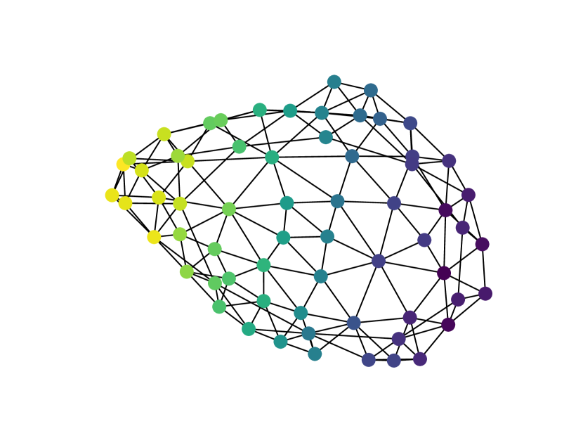
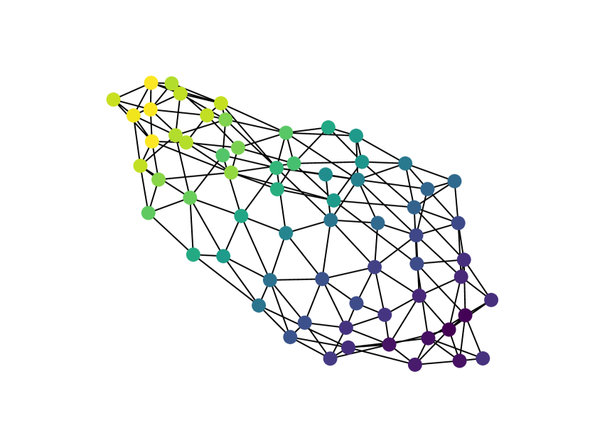
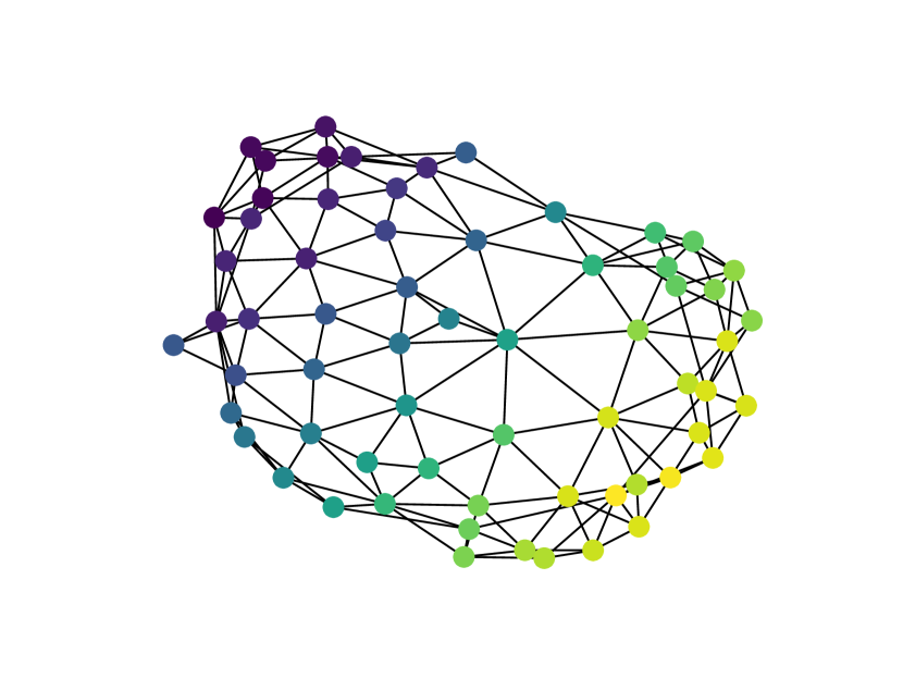
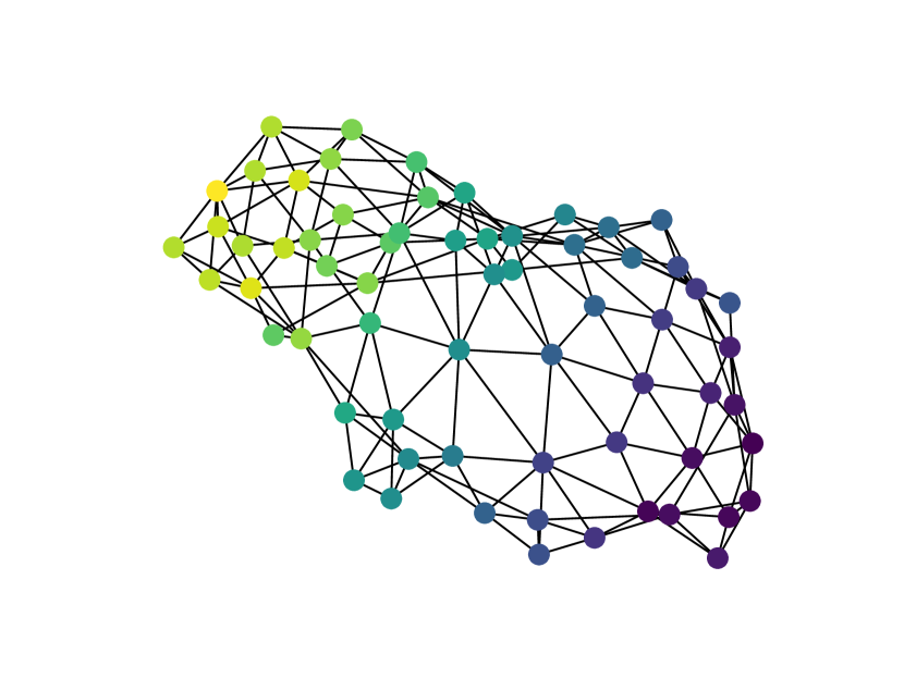
(a) Uncurated samples from ANFM model trained on expanded planar graph dataset.

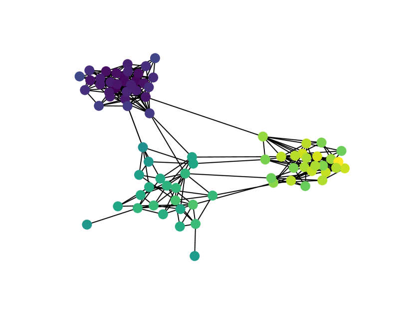
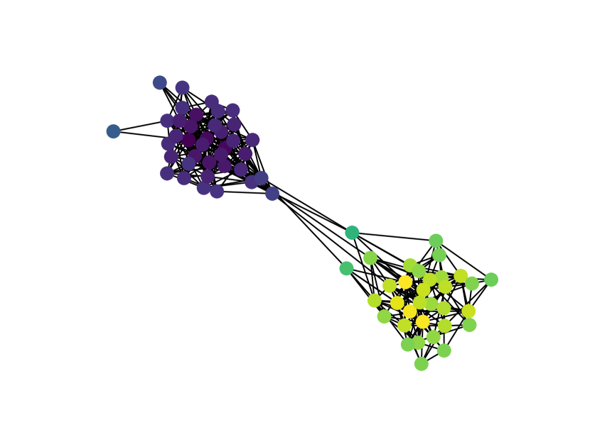
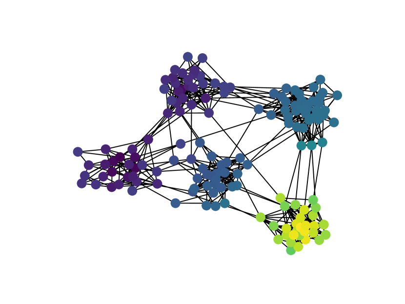
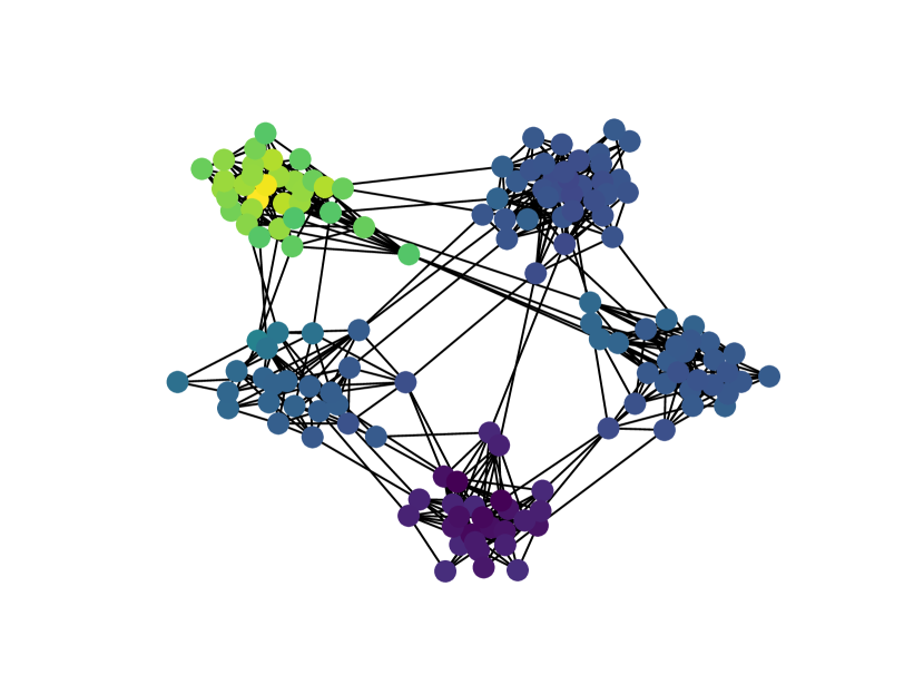
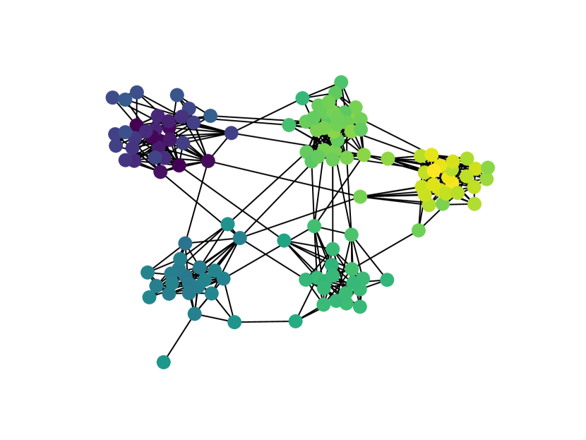
(b) Uncurated samples from ANFM model trained on expanded SBM dataset.

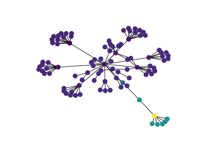
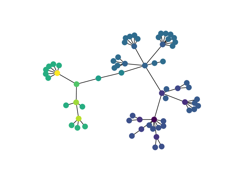
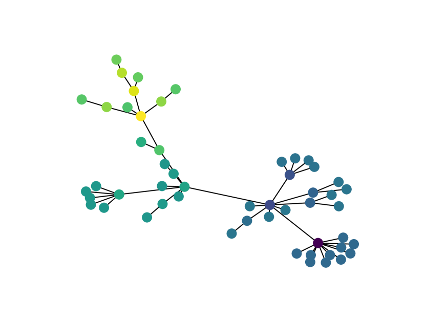
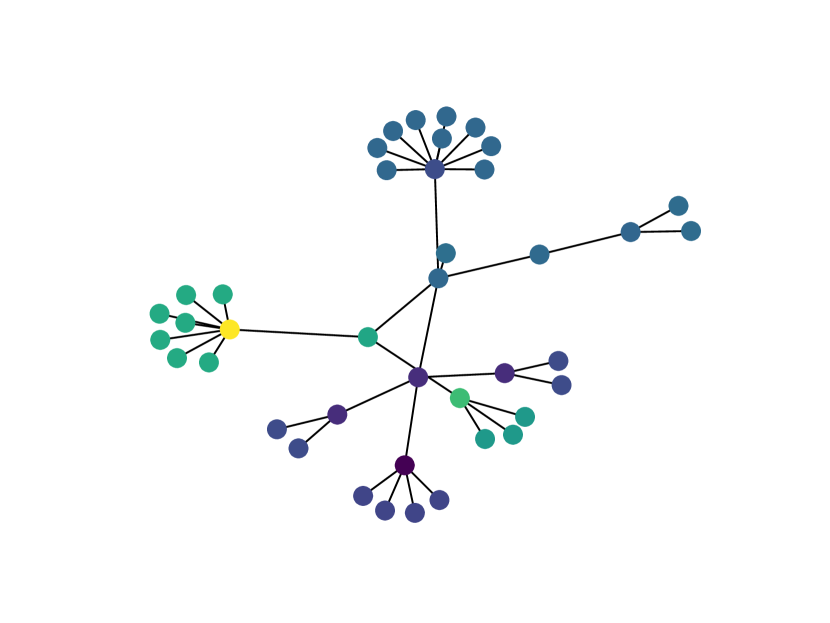
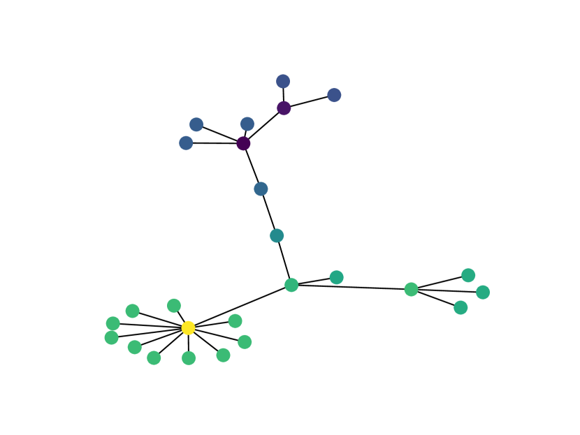
(c) Uncurated samples from ANFM model trained on expanded lobster dataset.

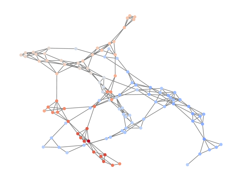
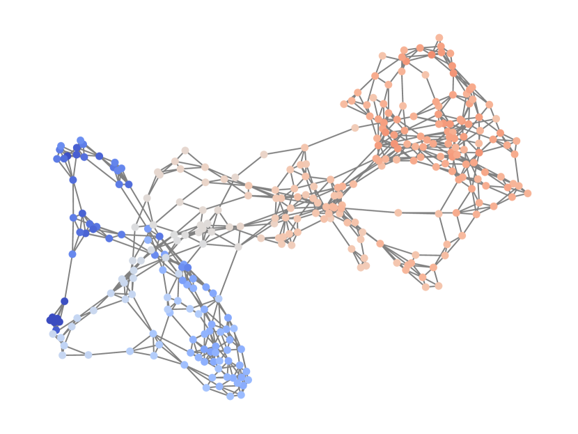
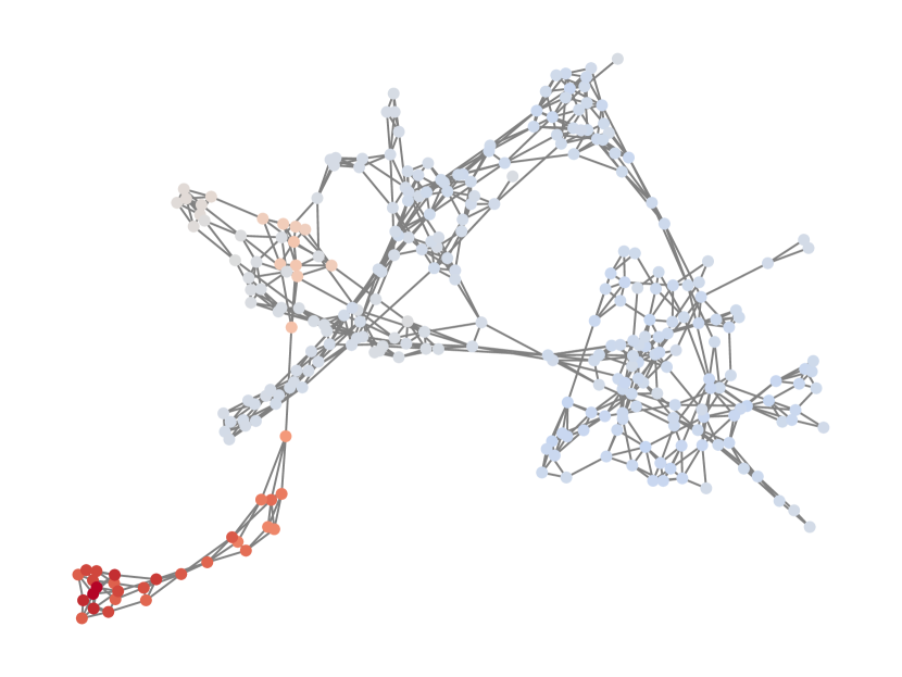
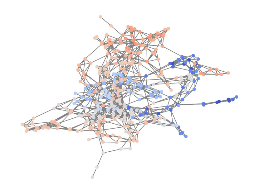
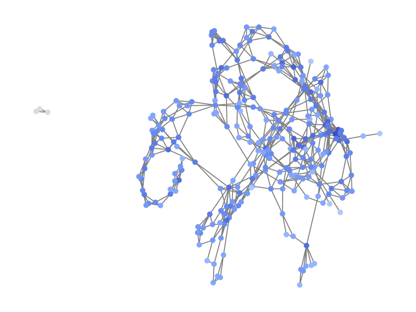
(d) Uncurated samples from ANFM model trained on protein dataset.

Figure 5: Uncurated samples from ANFM (line Fiedler variant).

Appendix H Baselines

H.1 GRAN Hyperparameters

For our experiments on the expanded lobster dataset, we use the hyperparameters provided by Liao et al. (2019) for their own (smaller) lobster dataset. For experiments on the expanded planar graph dataset, we utilize the same hyper-parameter setting but reduce the batchsize to 16. For experiments on the SBM dataset, we further reduce the batchsize to 8 and use 2 gradient accumulation steps. For the experiments on the protein dataset, we utilize the pretrained model provided at http://www.cs.toronto.edu/~rjliao/model/gran_DD.pth. We perform inference with a batch size of 20.

H.2 DiGress Hyperparameters

For our experiments on the expanded planar graph and SBM datasets, we use the hyperparameters provided by Vignac et al. (2023) for the corresponding SPECTRE datasets. On the lobster dataset, we use the same hyperparameters as for the expanded SBM dataset (8 layers and batch size 12). On the protein dataset, we use similar hyperparameters as for the expanded SBM dataset but reduce the batch size to 4 due to GPU memory constraints. We use the same inference approach as Vignac et al. (2023), performing generation with a batch size that is twice as large as the batch size used for training. In all cases, we follow Vignac et al. (2023) in using 1000 diffusion steps.

H.3 ESGG Hyperparameters

For our experiments on the expanded planar graph and SBM datasets, we use the hyperparameters provided by Bergmeister et al. (2024) for the corresponding SPECTRE datasets. For the expanded lobster dataset, we use the hyperparameters used by Bergmeister et al. (2024) for their tree dataset. We use the test batch sizes provided by Bergmeister et al. (2024) in their hyperparameter configurations.

H.4 GRAN Model Selection

Expanded Planar.

In Table 14, we present validation results of the GRAN model trained on the expanded planar graph dataset. We observe no clear development in model performance past 500 steps. We select the checkpoint at 1000 steps.

Table 14: Validation results for GRAN model trained on expanded planar graph dataset. Evaluated on 260 model samples.

# Steps	Valid $(\uparrow)$	Node Count $(\downarrow)$	Degree $(\downarrow)$	Clustering $(\downarrow)$	Orbit $(\downarrow)$	Spectral $(\downarrow)$
500	$0.0$	$0.006\,512\,842\,467\,044\,2$	$0.008\,655\,974\,681\,351\,486$	$0.174\,889\,231\,106\,533\,95$	$0.069\,325\,837\,542\,367\,99$	$0.009\,560\,386\,778\,039\,831$
1000	$0.0$	$0.000\,724\,716\,593\,736\,740\,6$	$0.007\,020\,969\,141\,104\,061$	$0.169\,566\,621\,898\,876\,14$	$0.110\,030\,338\,293\,784\,17$	$0.008\,597\,715\,607\,204\,348$
1500	$0.769\,23$	$0.009\,975\,041\,614\,635\,36$	$0.006\,600\,394\,482\,517\,924$	$0.172\,965\,201\,590\,015\,58$	$0.074\,266\,976\,799\,518\,99$	$0.007\,811\,115\,296\,344\,484$
2000	$0.0$	$0.002\,129\,057\,689\,464\,586\,3$	$0.005\,635\,743\,243\,073\,81$	$0.165\,837\,421\,503\,632\,95$	$0.081\,589\,192\,909\,273\,58$	$0.009\,418\,713\,734\,661\,965$
2500	$0.769\,23$	$0.003\,325\,483\,702\,043\,330\,3$	$0.006\,407\,487\,535\,491\,363$	$0.176\,780\,050\,429\,995\,12$	$0.104\,230\,495\,761\,535\,42$	$0.008\,729\,458\,835\,383\,674$

Expanded SBM.

In Table 15, we present validation results of the GRAN model trained on the expanded SBM dataset. We find that, overall, the checkpoint at 200 steps appears to perform best and select it.

Table 15: Validation results for GRAN model trained on expanded SBM dataset. Evaluated on 260 model samples.

# Steps	Valid $(\uparrow)$	Node Count $(\downarrow)$	Degree $(\downarrow)$	Clustering $(\downarrow)$	Orbit $(\downarrow)$	Spectral $(\downarrow)$
100	$22.307\,69$	$1.999\,246\,051\,529\,318\,2$	$0.024\,336\,402\,812\,597\,19$	$0.011\,925\,507\,279\,369\,45$	$0.039\,986\,394\,750\,644\,08$	$0.003\,666\,527\,824\,800\,924\,8$
200	$24.230\,77$	$1.999\,848\,082\,005\,887\,3$	$0.019\,381\,308\,189\,759\,14$	$0.011\,362\,735\,690\,513\,045$	$0.029\,006\,325\,466\,018\,848$	$0.002\,580\,012\,148\,128\,085\,8$
400	$20.384\,62$	$1.999\,937\,666\,739\,294$	$0.027\,753\,167\,613\,836\,95$	$0.012\,953\,346\,316\,353\,543$	$0.044\,755\,986\,747\,505\,055$	$0.003\,877\,968\,168\,626\,289$
600	$20.384\,62$	$1.999\,895\,209\,849\,309$	$0.022\,525\,270\,428\,906\,508$	$0.011\,991\,012\,316\,821\,065$	$0.031\,840\,088\,142\,903\,33$	$0.003\,008\,119\,156\,180\,155\,7$

Expanded Lobster.

In Table 16, we present validation results of the GRAN model trained on the expanded lobster dataset. We observe no improvement in validity past 2500 steps and select this checkpoint.

Table 16: Validation results for GRAN model trained on expanded lobster graph dataset. Evaluated on 260 model samples.

# Steps	Valid $(\uparrow)$	Node Count $(\downarrow)$	Degree $(\downarrow)$	Clustering $(\downarrow)$	Orbit $(\downarrow)$	Spectral $(\downarrow)$
500	$2.343\,75$	$2.0$	$0.025\,678\,888\,709\,036\,674$	$0.475\,289\,832\,156\,599\,6$	$0.250\,717\,413\,543\,497\,2$	$0.050\,883\,798\,214\,956\,366$
1500	$38.671\,88$	$2.0$	$0.009\,245\,991\,054\,127\,822$	$0.011\,162\,033\,113\,309\,988$	$0.162\,423\,729\,302\,631\,83$	$0.032\,874\,624\,407\,166\,93$
2500	$42.578\,12$	$2.0$	$0.008\,319\,556\,749\,788\,681$	$0.005\,881\,559\,653\,525\,548$	$0.174\,911\,126\,810\,097\,57$	$0.036\,088\,531\,002\,298\,474$
3500	$42.968\,75$	$2.0$	$0.010\,110\,533\,291\,801\,671$	$0.004\,942\,212\,659\,893\,919$	$0.196\,979\,611\,732\,978\,95$	$0.040\,606\,663\,114\,690\,41$

H.5 ESGG Model Selection

While ESGG maintains exponential moving averages of model weights during training, we choose to only evaluate non-smoothed model weights (i.e. the EMA weights with decay parameter $\gamma=1$), as validation is compute-intensive.

SBM Dataset.

In our experiments, we obtain worse performance on the expanded SBM dataset than was reported on the smaller SPECTRE SBM dataset in (Bergmeister et al., 2024). In Figure 6, we show the development of validity throughout training, which lasted over 4.5 days on an H100 GPU. Throughout training, we fail to match the validity reported in (Bergmeister et al., 2024). Although the validity estimate is quite noisy, it appears to plateau. We select a model checkpoint at 4.8M steps.

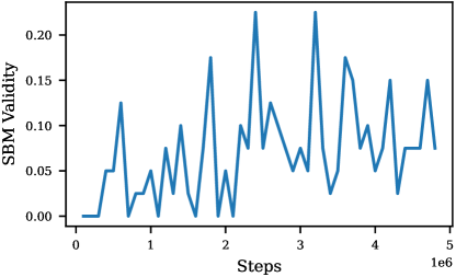
Figure 6: SBM validity during training of ESGG on expanded SBM dataset. Validity is computed using 1000 refinement steps in validation but 100 refinement steps during testing to remain consistent with other baselines.

Protein Dataset.

Model selection on the protein graph dataset is challenging, as the MMD metrics computed during validation are noisy, and generating model samples is time-consuming. We take a structured approach and evaluate model checkpoints at 1-4M training steps using the same validation approach as Bergmeister et al. (2024). Namely, for each graph in the validation set, we generate a corresponding model sample with the same number of nodes. We present the resulting MMD metrics in Table 17.

Table 17: Validation results of ESGG trained on protein dataset.

# Steps	Degree $(\downarrow)$	Clustering $(\downarrow)$	Orbit $(\downarrow)$	Spectral $(\downarrow)$	Wavelet $(\downarrow)$	Ratio $(\downarrow)$
1M	$0.024\,156\,044\,031\,717\,894$	$0.107\,433\,840\,514\,871\,07$	$0.109\,106\,189\,516\,502\,42$	$0.009\,494\,919\,139\,395\,597$	$0.026\,678\,779\,183\,871\,182$	$63.812\,166\,651\,441\,146$
2M	$0.002\,848\,594\,743\,062\,316$	$0.025\,364\,130\,117\,647\,946$	$0.051\,967\,623\,090\,149\,795$	$0.000\,911\,170\,215\,944\,334\,7$	$0.002\,257\,864\,938\,477\,016\,6$	$12.242\,573\,717\,269\,035$
3M	$0.006\,642\,071\,284\,827\,633$	$0.063\,219\,122\,287\,480\,4$	$0.063\,976\,415\,154\,167\,52$	$0.002\,995\,794\,518\,940\,497\,8$	$0.008\,999\,653\,206\,037\,24$	$23.620\,577\,496\,799\,804$
4M	$0.029\,305\,051\,173\,869\,945$	$0.101\,603\,821\,188\,956\,89$	$0.247\,438\,467\,558\,148\,47$	$0.007\,939\,929\,484\,529\,706$	$0.022\,371\,673\,726\,054\,864$	$84.998\,193\,609\,411\,02$

Based on these results, we select the model checkpoint at 2M steps.

Appendix I Additional Ablations

Noise Augmentation.

We ablate noise augmentation for the DFS variant of ANFM, supplementing the results previously reported in Table 5. We run 100k training steps of stage I with DFS filtrations on the expanded planar graph dataset and compare performance with and without noise augmentation. Consistent with our previous observations, we find in Table 18 that noise augmentation substantially boosts performance.

Table 18: Performance of DFS variant of AFNM after 100k steps of stage I training on expanded planar graph dataset with and without noise augmentation.

	Stage I w/ Noise	Stage I w/o Noise
VUN ($\uparrow$)	$2.246\,09$	$0.292\,97$
Degree ($\downarrow$)	$0.004\,992\,101\,268\,182\,836$	$0.038\,061\,201\,024\,169\,88$
Clustering ($\downarrow$)	$0.227\,525\,235\,933\,564\,86$	$0.313\,580\,679\,563\,174\,5$
Spectral ($\downarrow$)	$0.004\,911\,161\,050\,920\,265$	$0.016\,921\,752\,975\,664\,894$
Orbit ($\downarrow$)	$0.050\,371\,323\,887\,762\,33$	$0.104\,538\,064\,464\,774\,43$

GAN Tuning.

We supplement the results on the effectiveness of adversarial finetuning we presented in Table 5. In Table 19, we present ablation results for the DFS variant on the expanded planar graph dataset. In Tables 20 and 21, we compare models after training stage I and II on the expanded SBM and lobster datasets from Sec. 5.2. Again, we observe that adversarial fine-tuning substantially improves performance in terms of validity and MMD metrics.

Table 19: Performance of DFS variant of AFNM after stage I (200k steps) and stage II on expanded planar graph dataset. For results on Fiedler variant, see Table 5.

	Stage II	Stage I
VUN ($\uparrow$)	$45.605\,47$	$2.050\,78$
Degree ($\downarrow$)	$0.000\,312\,928\,398\,365\,608\,4$	$0.005\,736\,982\,906\,912\,713$
Clustering ($\downarrow$)	$0.029\,550\,210\,939\,678\,245$	$0.229\,718\,334\,555\,092\,66$
Spectral ($\downarrow$)	$0.001\,685\,905\,166\,112\,666\,7$	$0.005\,847\,635\,148\,975\,35$
Orbit ($\downarrow$)	$0.000\,444\,722\,907\,314\,787\,36$	$0.031\,798\,398\,099\,886\,16$

Table 20: Performance of ANFM models after stage I (200k steps) and stage II on expanded SBM dataset. Showing median $\pm$ maximum deviation across three runs for Fiedler variant and a single run for DFS variant. All models attain perfect uniqueness and novelty scores.

	Fiedler		DFS
	Stage II	Stage I	Stage II	Stage I
VUN ($\uparrow$)	$75.976\,56$ $\pm$ $3.710\,94$	$39.648\,44$ $\pm$ $4.6875$	$78.027\,34$	$22.851\,56$
Degree ($\downarrow$)	$0.001\,438\,607\,730\,545\,049\,5$ $\pm$ $0.006\,178\,398\,816\,857\,555$	$0.002\,263\,204\,775\,078\,797\,6$ $\pm$ $0.006\,340\,091\,250\,923\,940\,4$	$0.000\,794\,559\,290\,614\,893\,5$	$0.000\,402\,413\,470\,753\,426\,6$
Clustering ($\downarrow$)	$0.005\,062\,382\,182\,491\,599$ $\pm$ $0.000\,920\,277\,666\,189\,260\,6$	$0.008\,214\,422\,115\,318\,282$ $\pm$ $0.001\,244\,971\,202\,062\,648\,8$	$0.004\,853\,086\,793\,020\,355\,5$	$0.011\,657\,713\,271\,663\,664$
Spectral ($\downarrow$)	$0.001\,141\,348\,405\,031\,772\,4$ $\pm$ $0.000\,587\,345\,396\,197\,980\,2$	$0.003\,180\,424\,042\,823\,038$ $\pm$ $0.000\,633\,519\,854\,897\,457\,4$	$0.000\,813\,837\,757\,143\,165\,4$	$0.001\,994\,394\,062\,739\,601\,7$
Orbit ($\downarrow$)	$0.018\,009\,643\,354\,469\,057$ $\pm$ $0.017\,066\,125\,210\,734\,43$	$0.021\,046\,548\,899\,889\,94$ $\pm$ $0.013\,498\,147\,868\,981\,819$	$0.004\,919\,597\,001\,513\,051$	$0.039\,016\,947\,339\,730\,726$

Table 21: Performance of models after stage I (100k steps) and stage II on expanded lobster dataset. Showing median $\pm$ maximum deviation across three runs.

	Fiedler		DFS
	Stage II	Stage I	Stage II	Stage I
VUN ($\uparrow$)	$79.101\,56$ $\pm$ $7.128\,91$	$31.25$ $\pm$ $4.6875$	$87.597\,66$	$47.460\,94$
Degree ($\downarrow$)	$0.000\,403\,299\,865\,038\,953$ $\pm$ $0.001\,310\,165\,552\,012\,909\,6$	$0.000\,369\,015\,185\,874\,399\,5$ $\pm$ $0.000\,969\,749\,715\,219\,681$	$7.824\,159\,351\,721\,427\text{\times}{10}^{-05}$	$0.020\,871\,511\,968\,871\,38$
Clustering ($\downarrow$)	$7.888\,505\,157\,871\,428\text{\times}{10}^{-05}$ $\pm$ $5.322\,273\,966\,479\,329\,5\text{\times}{10}^{-05}$	$0.013\,616\,898\,759\,275\,742$ $\pm$ $0.005\,381\,368\,107\,876\,039$	$1.641\,427\,338\,494\,594\,3\text{\times}{10}^{-06}$	$0.004\,335\,325\,046\,007\,421$
Spectral ($\downarrow$)	$0.001\,578\,534\,329\,912\,617\,6$ $\pm$ $0.002\,789\,156\,743\,140\,397\,4$	$0.003\,015\,402\,469\,744\,632\,4$ $\pm$ $0.001\,204\,056\,581\,287\,86$	$0.000\,967\,362\,477\,460\,209\,6$	$0.011\,864\,433\,494\,173\,321$
Orbit ($\downarrow$)	$0.001\,043\,212\,982\,421\,16$ $\pm$ $0.015\,604\,136\,395\,777\,068$	$0.007\,331\,627\,279\,350\,661$ $\pm$ $0.002\,556\,116\,180\,955\,303\,5$	$0.000\,727\,856\,308\,562\,202\,5$	$0.020\,641\,683\,620\,304\,94$
Unique ($\uparrow$)	$99.804\,69$ $\pm$ $0.097\,66$	$99.511\,72$ $\pm$ $0.390\,62$	$99.707\,03$	$100.0$
Novel ($\uparrow$)	$100.0$ $\pm$ $0.097\,66$	$99.902\,34$ $\pm$ $0.390\,62$	$99.707\,03$	$99.902\,34$

Filtration Function.

In Table 22, we study alternative filtration functions. We compare the line fiedler function to centrality-based filtration functions. Following Anthonisse (1971); Brandes (2008), we let $\sigma(i,j)$ denote the number of shortest paths between two nodes $i,j\in V$, and $\sigma(i,j\,|\,e)$ denote the number of these paths passing through an edge $e\in E$. Then, we define the betweenness centrality function as:

$$f_{\text{between}}(e):=\sum_{i,j\in V}\frac{\sigma(i,j|e)}{\sigma(i,j)},\qquad\forall\>e\in E.$$ (29)

Based on this, we define the remoteness centrality as $f_{\mathrm{remote}}(e)=-f_{\mathrm{between}}(e)$. We use the same filtration scheduling approach as for the line Fiedler function. We observe that the line fiedler function appears to out-perform the two alternatives in our setting.

Table 22: Performance after training stage I with different filtration functions for 100k steps on expanded planar graph dataset. Showing median of three runs for spectral variant and one run each for betweenness and remoteness variants.

	VUN ($\uparrow$)	Degree ($\downarrow$)	Clustering ($\downarrow$)	Spectral ($\downarrow$)	Orbit ($\downarrow$)
Line Fiedler	$20.214\,84$	$0.005\,753\,176\,855\,113\,784$	$0.176\,845\,325\,553\,082$	$0.004\,760\,004\,557\,846\,642$	$0.012\,890\,572\,283\,490\,664$
DFS	$2.246\,09$	$0.004\,992\,101\,268\,182\,836$	$0.227\,525\,235\,933\,564\,86$	$0.004\,911\,161\,050\,920\,265$	$0.050\,371\,323\,887\,762\,33$
Betweenness	$0.195\,31$	$0.006\,936\,244\,140\,129\,277$	$0.272\,363\,954\,306\,979\,13$	$0.012\,404\,566\,920\,876\,325$	$0.080\,396\,472\,819\,318\,94$
Remoteness	$3.515\,62$	$0.013\,609\,126\,202\,943\,633$	$0.272\,008\,138\,529\,307\,8$	$0.008\,461\,575\,324\,258\,286$	$0.023\,358\,653\,218\,225\,056$

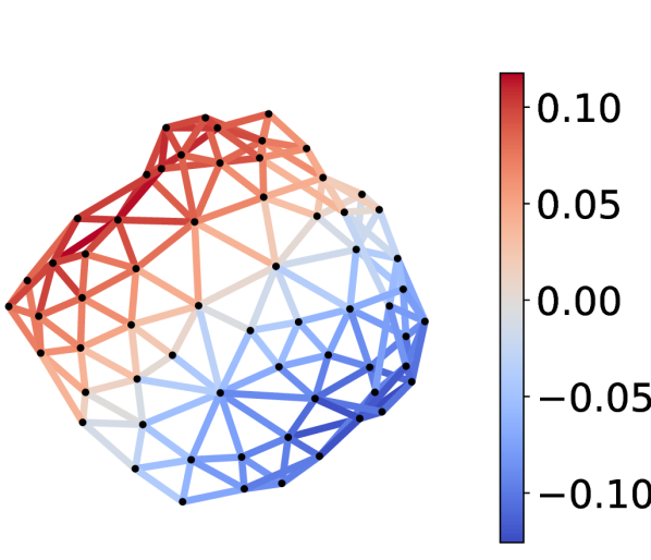
(a) Line Fiedler

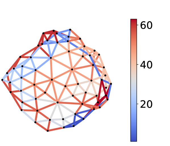
(b) DFS

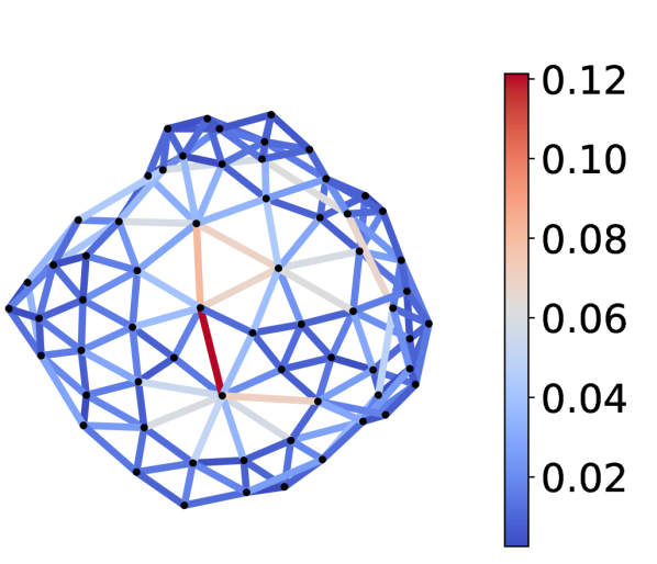
(c) Betweenness

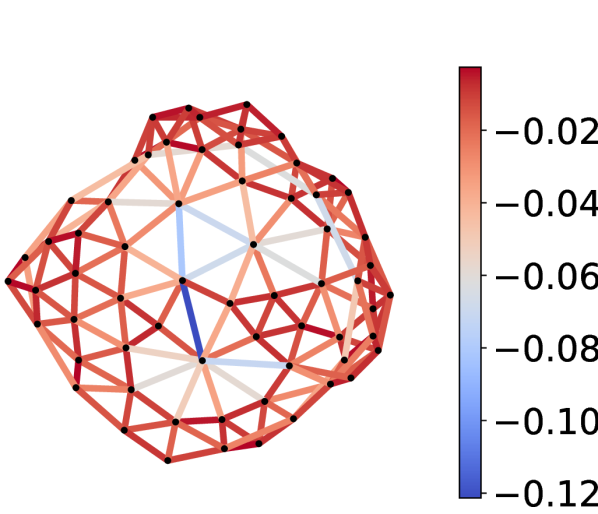
(d) Remoteness

Figure 7: Visualization of different filtration functions on a planar graph

Scheduling.

We recall that the filtration schedule of the line Fiedler variant depends on a mononotonically increasing function $\gamma:[0,1]\to[0,1]$. Here, we study the performance of the three choices for $\gamma$:

$$\mathrm{Linear:} \gamma(t):=t$$ (30)

$$\mathrm{Convex:} \gamma(t):=1-\cos\left(\frac{\pi t}{2}\right)$$

$$\mathrm{Concave:} \gamma(t):=\sin\left(\frac{\pi t}{2}\right)$$

We present results on the planar graph dataset in Table 23.

Table 23: Performance after training stage I with different filtration schedules for 100k steps on expanded planar graph dataset with line Fiedler variant. All models attain perfect uniqueness and novelty scores. Showing median of three runs for linear variant and one run each for convex and concave variants.

	VUN ($\uparrow$)	Degree ($\downarrow$)	Clustering ($\downarrow$)	Spectral ($\downarrow$)	Orbit ($\downarrow$)
Linear	$20.214\,84$	$0.005\,753\,176\,855\,113\,784$	$0.176\,845\,325\,553\,082$	$0.004\,760\,004\,557\,846\,642$	$0.012\,890\,572\,283\,490\,664$
Convex	$5.664\,06$	$0.004\,305\,953\,076\,664\,704$	$0.223\,913\,808\,151\,014\,36$	$0.003\,971\,669\,668\,414\,002$	$0.006\,236\,163\,601\,005\,318$
Concave	$31.054\,69$	$0.004\,511\,650\,594\,824\,834$	$0.158\,973\,040\,348\,968\,1$	$0.005\,904\,321\,479\,719\,421$	$0.015\,333\,300\,003\,760\,542$

We find that no single variant performs consistently best across all evaluation metrics. However, the concave variant attains the highest validity score.

Node Individualization.

In Table 24, we study different node individualization techniques for the line Fiedler variant of ANFM. We refer to the ordering scheme we describe in Appendix F.1 as the derived ordering, as it is based on the values of the line Fiedler filtration function. Additionally, we study random orderings and node orderings according to a depth first search (DFS). Moreover, we compare to node individualizations that do not consist of positional embeddings w.r.t. a node orderings but instead i.i.d. gaussian noise that is re-applied in each time-step. Finally, we also consider a variant in which no individualization is applied, i.e., the embedding matrix $W^{\mathrm{node}}$ is fixed to be all-zeros.

Table 24: Performance after training stage I of the line Fiedler variant with different node individualization techniques for 100k steps on expanded planar graph dataset. All models attain perfect uniqueness and novelty scores. Showing median of three runs for derived ordering and one run each for all other variants.

	VUN ($\uparrow$)	Degree ($\downarrow$)	Clustering ($\downarrow$)	Spectral ($\downarrow$)	Orbit ($\downarrow$)
Derived Ordering	$20.214\,84$	$0.005\,753\,176\,855\,113\,784$	$0.176\,845\,325\,553\,082$	$0.004\,760\,004\,557\,846\,642$	$0.012\,890\,572\,283\,490\,664$
DFS Ordering	$28.906\,25$	$0.005\,522\,729\,038\,354\,379$	$0.180\,285\,014\,958\,729\,4$	$0.002\,375\,462\,352\,541\,602$	$0.005\,295\,329\,680\,999\,883$
Random Ordering	$18.359\,38$	$0.008\,545\,819\,157\,682\,821$	$0.233\,231\,635\,534\,885\,05$	$0.002\,303\,345\,460\,326\,067\,2$	$0.009\,101\,400\,057\,227\,371$
Gaussian Noise	$12.988\,28$	$0.008\,574\,077\,006\,591\,851$	$0.235\,567\,890\,589\,987\,84$	$0.003\,107\,490\,343\,757\,568\,5$	$0.011\,190\,940\,174\,161\,002$
Zeros	$13.476\,56$	$0.005\,743\,729\,730\,228\,297\,5$	$0.219\,493\,523\,558\,580\,15$	$0.002\,304\,007\,587\,289\,991\,2$	$0.009\,091\,846\,763\,255\,473$

We find that individualizing nodes with learned embeddings based on some ordering (either random, derived from the line Fiedler filtration function, or a DFS search) appears to be beneficial. On the planar graph dataset, there is no clear benefit of the derived ordering over random orderings. However, we observe a clear advantage on the SBM dataset, as can be seen in Table 25.

Table 25: Performance after training stage I of the line Fiedler variant with derived and random node ordering after 100k steps on expanded SBM datasets. Showing median $\pm$ maximum deviation across three runs for derived ordering and one run for random ordering.

	Derived Ordering	Random Ordering
VUN ($\uparrow$)	$26.953\,12$ $\pm$ $2.636\,72$	$2.441\,41$
Degree ($\downarrow$)	$0.022\,242\,749\,862\,799\,06$ $\pm$ $0.012\,668\,181\,724\,511\,34$	$0.039\,554\,317\,170\,922\,95$
Clustering ($\downarrow$)	$0.010\,618\,129\,867\,799\,631$ $\pm$ $0.001\,212\,205\,398\,574\,237$	$0.012\,247\,080\,788\,020\,694$
Spectral ($\downarrow$)	$0.006\,077\,873\,147\,199\,542$ $\pm$ $0.001\,401\,568\,579\,899\,370\,4$	$0.014\,429\,714\,823\,977\,813$
Orbit ($\downarrow$)	$0.054\,785\,935\,142\,483\,41$ $\pm$ $0.024\,420\,373\,909\,542\,548$	$0.059\,555\,555\,123\,545\,73$
Unique ($\uparrow$)	$1.0$ $\pm$ $0.0$	$0.995\,117\,187\,5$
Novel ($\uparrow$)	$1.0$ $\pm$ $0.0$	$1.0$

Stage I.

While the ablation study in Sec. 5.4 demonstrates that stage II training substantially boosts performance, we now show that, similarly, stage I is crucial too. To this end, we perform stage II training on a very early checkpoint of stage I training. Specifically, we use a checkpoint obtained after 10k steps of stage I training on the expanded planar graph dataset with the line Fiedler variant. We present the results in Table 26. We observe that performing stage II training on a premature checkpoint from stage I substantially harms performance. Hence, stage I training is a crucial part of our method.

Table 26: Performance on expanded planar graph dataset of line Fiedler ANFM variant with different training durations during stage I. Showing median across three runs for 200k steps and a single run for 10k steps.

# Stage I Steps	VUN ($\uparrow$)	Deg. ($\downarrow$)	Clus. ($\downarrow$)	Orbit ($\downarrow$)	Spec. ($\downarrow$)
200k	$79.199\,22$	$0.000\,383\,280\,816\,482\,312\,05$	$0.018\,315\,733\,274\,652\,524$	$0.000\,188\,098\,802\,662\,350\,9$	$0.001\,198\,020\,860\,018\,855\,8$
10k	$3.320\,31$	$0.001\,552\,548\,097\,448\,758\,2$	$0.227\,808\,118\,011\,291\,08$	$0.046\,382\,451\,203\,791\,586$	$0.006\,925\,660\,029\,444\,058\,5$

Appendix J Bias and Variance of Estimators

Previous works (Martinkus et al., 2022; Vignac et al., 2023; Bergmeister et al., 2024) evaluate their graph generative models on as few as 40 samples. In this section, we investigate how this practice impacts the variance and bias of the estimators used in model evaluation and argue that a higher number of test samples should be chosen.

J.1 Variance of Validity Estimation

On synthetic datasets such as those introduced in (Martinkus et al., 2022), one may verify whether model samples are ”valid”, i.e., whether they satisfy a property that is fulfilled by (almost) all samples of the true data distribution. By taking the ratio of valid graphs out of $n$ model samples, previous works have estimated the probability of obtaining valid graphs from the generator.

Definition J.1.

Let the random variable $G$ denote a sample from a graph generative model and let $\operatorname{valid}:\mathcal{G}\to\{0,1\}$ a measurable binary function that determines whether a sample is valid. Then the models true validity ratio is defined as:

$$\mathbb{P}[\operatorname{valid}(G)=1]$$ (31)

For i.i.d. samples $G_{1},\dots,G_{n}$, we introduce the following estimator:

$$V:=\frac{\sum_{i=1}^{n}\operatorname{valid}(G_{i})}{n}$$ (32)

Given the simplicity of the validity metric, we can very easily derive the uncertainty of the estimator used for evaluation. We make this concrete in Proposition J.2.

Proposition J.2.

For a generative model with a true validity ratio of $p\in[0,1]$, the validity estimator on $n$ samples is unbiased and has standard deviation $\sqrt{p(1-p)}/\sqrt{n}$.

Proof.

Assuming that the random variables $G_{1},\dots,G_{n}$ are i.i.d. samples from the generative model, then the random variables $\operatorname{valid}(G_{1}),\dots,\operatorname{valid}(G_{n})$ are i.i.d. according to $\operatorname{Bernoulli}(p)$. The validity estimator is given as:

$$V=\frac{\sum_{i=1}^{n}\operatorname{valid}(G_{i})}{n}$$ (33)

By the linearity of expectation, we have

$$\mathbb{E}[V]=\frac{\sum_{i=1}^{n}\mathbb{E}[\operatorname{valid}(G_{i})]}{n}=\frac{np}{p}=p$$ (34)

which shows that the estimator is unbiased. The variance is given by:

$$\mathrm{Var}[V] =\frac{\mathrm{Var}\left[\sum_{i=1}^{n}\operatorname{valid}(G_{i})\right]}{n^{2}}=\frac{\sum_{i=1}^{n}\mathrm{Var}[\operatorname{valid}(G_{i})]}{n^{2}}$$ (35)

$$=\frac{p(1-p)}{n}$$

where we used the independence assumption in the first line. Taking the square root, we obtain the standard deviation from the proposition. ∎

From Proposition J.2, we note that the standard deviation of the validity estimate can be as high as $1/(2\sqrt{n})$, which is achieved at $p=0.5$. For $n=40$, we find that the standard deviation can therefore be as high as $7.9$ percentage points.

J.2 Bias and Variance of MMD Estimation

Definition J.3.

Let $(\mathcal{X},d)$ be a metric space and let $k:\mathcal{X}\times\mathcal{X}\to\mathbb{R}$ be a measurable, symmetric kernel which is bounded but not necessarily positive-definite. Let $X:=[x_{1},\dots,x_{n}]$ be i.i.d. samples from a Borel distribution $p_{x}$ on $\mathcal{X}$ and $Y:=[y_{1},\dots,y_{n}]$ be i.i.d. samples from a distribution $p_{y}$. Assume $X$ and $Y$ to be independent. Following (Gretton et al., 2012), define the squared MMD of $p_{x}$ and $p_{y}$ as:

$$\mathrm{MMD}^{2}(p_{x},p_{y}):=\mathbb{E}[k(x_{1},x_{2})]+\mathbb{E}[k(y_{1},y_{2})]-2\mathbb{E}[k(x_{1},y_{1})]$$ (36)

and note that this is well-defined by our assumptions. Finally, introduce the following estimator for the squared MMD:

$$M:=\frac{1}{n^{2}}\sum_{i,j=1}^{n}k(x_{i},x_{j})+\frac{1}{m^{2}}\sum_{i,j=1}^{m}k(y_{i},y_{j})-\frac{2}{nm}\sum_{i=1}^{n}\sum_{j=1}^{m}k(x_{i},y_{j})$$ (37)

We empirically study bias and variance of the MMD estimates on the planar graph dataset. We generate 8192 samples from one of our trained model and repeatedly compute the MMD between the test set and a random subset of those samples. We vary the size of the random subsets and run 64 evaluations for each size, computing mean and standard deviation of the MMD metrics across the 64 evaluations. We report the results in Table 27.

Table 27: Mean MMD $\pm$ standard deviation across 64 evaluation runs of a single model. The test set contains 256 planar graphs, while a varying number of model samples is used, as indicated on the left. The MMD and its variance decrease substantially with larger numbers of model samples.

# Model Samples	Degree $(\downarrow)$	Clustering $(\downarrow)$	Spectral $(\downarrow)$
32	$8.59\text{\times}{10}^{-04}$ $\pm$ $5.59\text{\times}{10}^{-04}$	$4.21\text{\times}{10}^{-02}$ $\pm$ $1.44\text{\times}{10}^{-02}$	$4.73\text{\times}{10}^{-03}$ $\pm$ $9.14\text{\times}{10}^{-04}$
64	$5.58\text{\times}{10}^{-04}$ $\pm$ $2.90\text{\times}{10}^{-04}$	$2.68\text{\times}{10}^{-02}$ $\pm$ $7.58\text{\times}{10}^{-03}$	$2.59\text{\times}{10}^{-03}$ $\pm$ $4.78\text{\times}{10}^{-04}$
128	$4.40\text{\times}{10}^{-04}$ $\pm$ $1.79\text{\times}{10}^{-04}$	$2.17\text{\times}{10}^{-02}$ $\pm$ $4.33\text{\times}{10}^{-03}$	$1.61\text{\times}{10}^{-03}$ $\pm$ $3.16\text{\times}{10}^{-04}$
256	$4.39\text{\times}{10}^{-04}$ $\pm$ $1.45\text{\times}{10}^{-04}$	$2.02\text{\times}{10}^{-02}$ $\pm$ $3.89\text{\times}{10}^{-03}$	$1.14\text{\times}{10}^{-03}$ $\pm$ $1.86\text{\times}{10}^{-04}$
512	$4.32\text{\times}{10}^{-04}$ $\pm$ $8.48\text{\times}{10}^{-05}$	$1.81\text{\times}{10}^{-02}$ $\pm$ $2.56\text{\times}{10}^{-03}$	$1.18\text{\times}{10}^{-03}$ $\pm$ $2.04\text{\times}{10}^{-04}$
1024	$4.26\text{\times}{10}^{-04}$ $\pm$ $5.99\text{\times}{10}^{-05}$	$1.72\text{\times}{10}^{-02}$ $\pm$ $1.66\text{\times}{10}^{-03}$	$1.18\text{\times}{10}^{-03}$ $\pm$ $2.00\text{\times}{10}^{-04}$

We observe that on average the MMD is severly over-estimated when using fewer than 256 model samples. At the same time, the variance between evaluation runs is large when few samples are used, making the results unreliable.

Appendix K Adversarial Finetuning Details

We provide pseudocode for the adversarial fine-tuning stage in Algorithm 1. We note that we do not make all procedures explicit and that many hyper-parameters must be chosen (including the number of steps and epochs in TrainGeneratorAndValueModel).

Generator.

The generator operates in inference mode, meaning that all dropout layers are disabled and batch normalization modules utilize the (now frozen) moving averages from training stage I. Hence, the behavior of the generative model becomes reproducible. It acts as a stochastic policy in a higher-order MDP, where the graphs $G_{0},\dots,G_{T}$ are the states. It receives a terminal reward for the plausibility of the final sample $G_{T}$.

Discriminator.

The discriminator is implemented as a GraphGPS (Rampásek et al., 2022) model which performs binary classification on graph samples $G_{T}$, distinguishing real samples from generated samples. It is trained via binary cross-entropy on batches consisting in equal proportions of generated graphs and graphs from the dataset $\mathcal{D}$. For a given graph $G_{T}$, the discriminator produces a probability of ”realness” by applying the sigmoid function to its logit. Following SeqGAN (Yu et al., 2017), the log-sigmoid of the logit then acts as a terminal reward for the generative model. We emphasize that only the final graph $G_{T}$ is presented to the discriminator.

Value Model.

The value model uses the same backbone architecture as our generative model and regresses scalars from pooled node representations. It is trained via least squares regression. The value model is used to compute baselined reward-to-go values.

Training Outline.

While Algorithm 1 provides a technical description of the training algorithm, we also provide a rougher outline here. At the start of training stage II, the generator is initialized with the weights learned in training stage I, while the discriminator and value model are initialized randomly. Before entering the main training loop, we pre-train discriminator and value model to match the generator. Namely, we first pre-train the discriminator to classify graphs as either ”real” or ”generated”. The log-likelihood of ”realness” acts as a terminal reward of the generative model. The discriminator is then pre-trained to regress the reward-to-go. After pre-training is finished, we proceed to the training loop, which consists of alternating training of (i) the generator and value model and (ii) the discriminator. As described above, the generator is trained via PPO to maximize the terminal reward provided by the discriminator. The value model is used to baseline the reward and is continuously trained to regress the reward-to-go. The discriminator, on the other hand, continues to be trained on generated and real graph samples via binary cross-entropy.

Algorithm 1 Adversarial Finetuning

TrainGeneratorAndValueModel$p_{\theta}$, $d_{\varphi}$, $v_{\vartheta}$$i=1\dots,N_{\mathrm{steps}}$$\mathcal{S}\leftarrow[\>]$List of sampled filtrations $r\leftarrow 0\>\in\>\mathbb{R}^{N_{\mathrm{samples}}}$Terminal rewards $j=1\dots,N_{\mathrm{samples}}$$G_{0}^{(j)},\dots,G_{T}^{(j)}\leftarrow\Call{SampleFiltration}{p_{\theta}}$$\mathcal{S}\operatorname{.append}\left(\left(G_{0}^{(j)},\dots,G_{T}^{(j)}\right)\right)$$r_{j}\leftarrow\operatorname{logsigmoid}(d_{\varphi}(G_{T}^{(j)}))$$r_{j}\leftarrow\max(r_{j},R_{\mathrm{lower}})$Reward clamping $r\leftarrow\Call{Whiten}{r}$Whiten rewards using EMA of mean and std $g_{j,t}\leftarrow 0\qquad\forall j=1,\dots,N_{\mathrm{samples}}\>\forall t=0,\dots,T-1$Rewards-to-go $j=1\dots,N_{\mathrm{samples}}$$t=0,\dots,T-1$$g_{j,t}\leftarrow r_{j}-v_{\vartheta}(G_{0}^{(j)},\dots,G_{t}^{(j)})$Compute baselined RTG $\Call{TrainValueModel}{v_{\vartheta},\mathcal{S},r}$$k=1\dots,N_{\mathrm{epoch}}$$l_{j,t}^{(k)}\leftarrow-\log p_{\theta}(G_{t}^{(j)}|G_{t-1}^{(j)},\dots,G_{0}^{(j)})\qquad\forall j=1,\dots,N_{\mathrm{samples}}\quad\forall t=1,\dots,T$$u_{j,t}\leftarrow\exp(\operatorname{sg}[l_{j,t}^{(1)}]-l_{j,t}^{(k)})\qquad\forall j,t$$\mathcal{L}_{j,t}^{(1)}\leftarrow-u_{j,t}\cdot g_{j,t-1}\qquad\forall j,t$$\mathcal{L}_{j,t}^{(2)}\leftarrow-\operatorname{clamp}(u_{j,t},1-\epsilon,1+\epsilon)\cdot g_{j,t-1}\qquad\forall j,t$$\mathcal{L}\leftarrow\sum_{j,t}\max(\mathcal{L}_{j,t}^{(1)},\mathcal{L}_{j,t}^{(2)})$$\theta\leftarrow\theta-\delta\nabla_{\theta}\mathcal{L}$Backpropagate and update parameters GANTuning$p_{\theta}$, $\mathcal{D}$Takes generator from training stage I and graph dataset $d_{\varphi}\leftarrow$new GNN Initialize discriminator $\Call{TrainDiscriminator}{p_{\theta},d_{\varphi},\mathcal{D}}$Pre-train discriminator $v_{\vartheta}\leftarrow$new mixer model $\mathcal{S}\leftarrow\Call{GenerateFiltrations}{p_{\theta}}$$r\leftarrow\Call{GradeSamples}{\mathcal{S},d_{\varphi}}$$\Call{TrainValueModel}{v_{\vartheta},\mathcal{S},r}$Pre-train value model not converged $\Call{TrainGeneratorAndValueModel}{p_{\theta},d_{\varphi},v_{\vartheta}}$$\Call{TrainDiscriminator}{p_{\theta},d_{\varphi},\mathcal{D}}$

References

- Anthonisse (1971) Anthonisse, J. M. The rush in a directed graph. Tech. Rep. BN 9/71, Stichting Mathematisch Centrum, 2e Boerhaavestraat 49, Amsterdam, October 1971.
- Austin et al. (2021) Austin, J., Johnson, D. D., Ho, J., Tarlow, D., and van den Berg, R. Structured denoising diffusion models in discrete state-spaces. In Advances in Neural Information Processing Systems 34 (NeurIPS), pp. 17981–17993, 2021.
- Bacciu et al. (2020) Bacciu, D., Micheli, A., and Podda, M. Edge-based sequential graph generation with recurrent neural networks. Neurocomputing, 416:177–189, 2020. doi: 10.1016/J.NEUCOM.2019.11.112.
- Bengio et al. (2015) Bengio, S., Vinyals, O., Jaitly, N., and Shazeer, N. Scheduled sampling for sequence prediction with recurrent neural networks. In Advances in Neural Information Processing Systems 28 (NeurIPS), pp. 1171–1179, 2015.
- Bergmeister et al. (2024) Bergmeister, A., Martinkus, K., Perraudin, N., and Wattenhofer, R. Efficient and scalable graph generation through iterative local expansion. In International Conference on Learning Representations (ICLR), 2024.
- Bojchevski et al. (2018) Bojchevski, A., Shchur, O., Zügner, D., and Günnemann, S. Netgan: Generating graphs via random walks. In International Conference on Machine Learning (ICML), volume 80 of Proceedings of Machine Learning Research, pp. 609–618. PMLR, 2018.
- Brandes (2008) Brandes, U. On variants of shortest-path betweenness centrality and their generic computation. Soc. Networks, 30(2):136–145, 2008. doi: 10.1016/J.SOCNET.2007.11.001.
- Brown et al. (2019) Brown, N., Fiscato, M., Segler, M. H., and Vaucher, A. C. Guacamol: benchmarking models for de novo molecular design. Journal of chemical information and modeling, 59(3):1096–1108, 2019.
- Cao & Kipf (2018) Cao, N. D. and Kipf, T. Molgan: An implicit generative model for small molecular graphs. CoRR, abs/1805.11973, 2018. URL http://arxiv.org/abs/1805.11973.
- Chen et al. (2022) Chen, D., O’Bray, L., and Borgwardt, K. M. Structure-aware transformer for graph representation learning. In International Conference on Machine Learning (ICML), volume 162 of Proceedings of Machine Learning Research, pp. 3469–3489. PMLR, 2022.
- Chen et al. (2023) Chen, X., He, J., Han, X., and Liu, L. Efficient and degree-guided graph generation via discrete diffusion modeling. In International Conference on Machine Learning (ICML), volume 202 of Proceedings of Machine Learning Research, pp. 4585–4610. PMLR, 2023.
- Dobson & Doig (2003) Dobson, P. D. and Doig, A. J. Distinguishing enzyme structures from non-enzymes without alignments. J. Mol. Biol., 330(4):771–783, July 2003.
- Dwivedi et al. (2022) Dwivedi, V. P., Luu, A. T., Laurent, T., Bengio, Y., and Bresson, X. Graph neural networks with learnable structural and positional representations. In The Tenth International Conference on Learning Representations (ICLR). OpenReview.net, 2022.
- Dwivedi et al. (2023) Dwivedi, V. P., Joshi, C. K., Luu, A. T., Laurent, T., Bengio, Y., and Bresson, X. Benchmarking graph neural networks. Journal of Machine Learning Research (JMLR), 24:43:1–43:48, 2023.
- Edelsbrunner et al. (2002) Edelsbrunner, Letscher, and Zomorodian. Topological persistence and simplification. Discrete & Computational Geometry, 28(4):511–533, Nov 2002. ISSN 1432-0444. doi: 10.1007/s00454-002-2885-2.
- Gangwal et al. (2024) Gangwal, A., Ansari, A., Ahmad, I., Azad, A. K., Kumarasamy, V., Subramaniyan, V., and Wong, L. S. Generative artificial intelligence in drug discovery: basic framework, recent advances, challenges, and opportunities. Frontiers in Pharmacology, 15:1331062, 2024.
- Gentile et al. (2022) Gentile, F., Yaacoub, J. C., Gleave, J., Fernandez, M., Ton, A.-T., Ban, F., Stern, A., and Cherkasov, A. Artificial intelligence–enabled virtual screening of ultra-large chemical libraries with deep docking. Nature Protocols, 17(3):672–697, Mar 2022. ISSN 1750-2799. doi: 10.1038/s41596-021-00659-2.
- Gómez-Bombarelli et al. (2016) Gómez-Bombarelli, R., Aguilera-Iparraguirre, J., Hirzel, T. D., Duvenaud, D., Maclaurin, D., Blood-Forsythe, M. A., Chae, H. S., Einzinger, M., Ha, D.-G., Wu, T., Markopoulos, G., Jeon, S., Kang, H., Miyazaki, H., Numata, M., Kim, S., Huang, W., Hong, S. I., Baldo, M., Adams, R. P., and Aspuru-Guzik, A. Design of efficient molecular organic light-emitting diodes by a high-throughput virtual screening and experimental approach. Nature Materials, 15(10):1120–1127, Oct 2016. ISSN 1476-4660. doi: 10.1038/nmat4717.
- Goyal et al. (2020) Goyal, N., Jain, H. V., and Ranu, S. Graphgen: A scalable approach to domain-agnostic labeled graph generation. In WWW ’20: The Web Conference 2020, pp. 1253–1263. ACM / IW3C2, 2020. doi: 10.1145/3366423.3380201.
- Gretton et al. (2012) Gretton, A., Borgwardt, K. M., Rasch, M. J., Schölkopf, B., and Smola, A. J. A kernel two-sample test. Journal of Machine Learning Research (JMLR), 13:723–773, 2012. doi: 10.5555/2503308.2188410.
- Grisoni et al. (2021) Grisoni, F., Huisman, B. J., Button, A. L., Moret, M., Atz, K., Merk, D., and Schneider, G. Combining generative artificial intelligence and on-chip synthesis for de novo drug design. Science Advances, 7(24):eabg3338, 2021.
- Hagberg et al. (2008) Hagberg, A., Swart, P., and Chult, D. Exploring network structure, dynamics, and function using networkx. In Proceedings of the 7th Python in Science Conference, 06 2008. doi: 10.25080/TCWV9851.
- Hu et al. (2020) Hu, W., Liu, B., Gomes, J., Zitnik, M., Liang, P., Pande, V. S., and Leskovec, J. Strategies for pre-training graph neural networks. In International Conference on Learning Representations (ICLR), 2020.
- Ingraham et al. (2019) Ingraham, J., Garg, V. K., Barzilay, R., and Jaakkola, T. S. Generative models for graph-based protein design. In Advances in Neural Information Processing Systems 32 (NeurIPS), pp. 15794–15805, 2019.
- Jo et al. (2022) Jo, J., Lee, S., and Hwang, S. J. Score-based generative modeling of graphs via the system of stochastic differential equations. In International Conference on Machine Learning (ICML), volume 162 of Proceedings of Machine Learning Research, pp. 10362–10383. PMLR, 2022.
- Karami (2024) Karami, M. Higen: Hierarchical graph generative networks. In International Conference on Learning Representations (ICLR), 2024.
- Kingma & Ba (2015) Kingma, D. P. and Ba, J. Adam: A method for stochastic optimization. In International Conference on Learning Representations (ICLR), 2015.
- Kingma & Welling (2014) Kingma, D. P. and Welling, M. Auto-encoding variational bayes. In International Conference on Learning Representations (ICLR), 2014.
- Kipf & Welling (2016) Kipf, T. N. and Welling, M. Variational graph auto-encoders. CoRR, abs/1611.07308, 2016. URL http://arxiv.org/abs/1611.07308.
- Kong et al. (2023) Kong, L., Cui, J., Sun, H., Zhuang, Y., Prakash, B. A., and Zhang, C. Autoregressive diffusion model for graph generation. In International Conference on Machine Learning (ICML), volume 202 of Proceedings of Machine Learning Research, pp. 17391–17408. PMLR, 2023.
- Kwon et al. (2020) Kwon, Y., Lee, D., Choi, Y.-S., Shin, K., and Kang, S. Compressed graph representation for scalable molecular graph generation. Journal of Cheminformatics, 12(1):58, Sep 2020. ISSN 1758-2946. doi: 10.1186/s13321-020-00463-2.
- Levinthal (1969) Levinthal, C. How to fold graciously. In Mossbauer Spectroscopy in Biological Systems: Proceedings of a meeting held at Allerton House, Monticello, Illinois., 1969. URL https://api.semanticscholar.org/CorpusID:9923873.
- Li et al. (2018) Li, Y., Vinyals, O., Dyer, C., Pascanu, R., and Battaglia, P. W. Learning deep generative models of graphs. CoRR, abs/1803.03324, 2018. URL http://arxiv.org/abs/1803.03324.
- Li et al. (2020) Li, Y., Hu, J., Wang, Y., Zhou, J., Zhang, L., and Liu, Z. Deepscaffold: A comprehensive tool for scaffold-based de novo drug discovery using deep learning. Journal of Chemical Information and Modeling, 60(1):77–91, Jan 2020. ISSN 1549-9596. doi: 10.1021/acs.jcim.9b00727.
- Liao et al. (2019) Liao, R., Li, Y., Song, Y., Wang, S., Hamilton, W. L., Duvenaud, D., Urtasun, R., and Zemel, R. S. Efficient graph generation with graph recurrent attention networks. In Advances in Neural Information Processing Systems 32 (NeurIPS), pp. 4257–4267, 2019.
- Liu et al. (2018) Liu, Q., Allamanis, M., Brockschmidt, M., and Gaunt, A. L. Constrained graph variational autoencoders for molecule design. In Advances in Neural Information Processing Systems 31 (NeurIPS), pp. 7806–7815, 2018.
- Liu et al. (2024) Liu, Y., Du, C., Pang, T., Li, C., Chen, W., and Lin, M. Graph diffusion policy optimization. CoRR, abs/2402.16302, 2024. doi: 10.48550/ARXIV.2402.16302.
- Martinkus et al. (2022) Martinkus, K., Loukas, A., Perraudin, N., and Wattenhofer, R. SPECTRE: spectral conditioning helps to overcome the expressivity limits of one-shot graph generators. In International Conference on Machine Learning (ICML), volume 162 of Proceedings of Machine Learning Research, pp. 15159–15179. PMLR, 2022.
- Mazuz et al. (2023) Mazuz, E., Shtar, G., Shapira, B., and Rokach, L. Molecule generation using transformers and policy gradient reinforcement learning. Scientific Reports, 13(1):8799, May 2023. ISSN 2045-2322. doi: 10.1038/s41598-023-35648-w.
- Niu et al. (2020) Niu, C., Song, Y., Song, J., Zhao, S., Grover, A., and Ermon, S. Permutation invariant graph generation via score-based generative modeling. In The 23rd International Conference on Artificial Intelligence and Statistics (AISTATS), volume 108 of Proceedings of Machine Learning Research, pp. 4474–4484. PMLR, 2020.
- O’Bray et al. (2021) O’Bray, L., Rieck, B., and Borgwardt, K. M. Filtration curves for graph representation. In KDD ’21: The 27th ACM SIGKDD Conference on Knowledge Discovery and Data Mining, Virtual Event, pp. 1267–1275. ACM, 2021. doi: 10.1145/3447548.3467442.
- Perez et al. (2018) Perez, E., Strub, F., de Vries, H., Dumoulin, V., and Courville, A. C. Film: Visual reasoning with a general conditioning layer. In Proceedings of the Thirty-Second AAAI Conference on Artificial Intelligence, (AAAI-18), the 30th innovative Applications of Artificial Intelligence (IAAI-18), and the 8th AAAI Symposium on Educational Advances in Artificial Intelligence (EAAI-18), pp. 3942–3951. AAAI Press, 2018. doi: 10.1609/AAAI.V32I1.11671.
- Polishchuk et al. (2013) Polishchuk, P. G., Madzhidov, T. I., and Varnek, A. Estimation of the size of drug-like chemical space based on GDB-17 data. Journal of Computer-Aided Molecular Design, 27(8):675–679, August 2013.
- Rampásek et al. (2022) Rampásek, L., Galkin, M., Dwivedi, V. P., Luu, A. T., Wolf, G., and Beaini, D. Recipe for a general, powerful, scalable graph transformer. In Advances in Neural Information Processing Systems 35 (NeurIPS), 2022.
- Ranzato et al. (2016) Ranzato, M., Chopra, S., Auli, M., and Zaremba, W. Sequence level training with recurrent neural networks. In International Conference on Learning Representations (ICLR), 2016.
- Schulman et al. (2017) Schulman, J., Wolski, F., Dhariwal, P., Radford, A., and Klimov, O. Proximal policy optimization algorithms. CoRR, abs/1707.06347, 2017. URL http://arxiv.org/abs/1707.06347.
- Schulz et al. (2022) Schulz, T. H., Welke, P., and Wrobel, S. Graph filtration kernels. In Thirty-Sixth AAAI Conference on Artificial Intelligence, AAAI 2022, Thirty-Fourth Conference on Innovative Applications of Artificial Intelligence, IAAI 2022, The Twelveth Symposium on Educational Advances in Artificial Intelligence, EAAI 2022, pp. 8196–8203. AAAI Press, 2022. doi: 10.1609/AAAI.V36I8.20793.
- Simonovsky & Komodakis (2018) Simonovsky, M. and Komodakis, N. Graphvae: Towards generation of small graphs using variational autoencoders. In 27th International Conference on Artificial Neural Networks (ICANN), Proceedings, Part I, volume 11139 of Lecture Notes in Computer Science, pp. 412–422. Springer, 2018. doi: 10.1007/978-3-030-01418-6“˙41.
- Southern et al. (2023) Southern, J., Wayland, J., Bronstein, M. M., and Rieck, B. Curvature filtrations for graph generative model evaluation. In Advances in Neural Information Processing Systems 36 (NeurIPS), 2023.
- Srivastava et al. (2014) Srivastava, N., Hinton, G. E., Krizhevsky, A., Sutskever, I., and Salakhutdinov, R. Dropout: a simple way to prevent neural networks from overfitting. Journal of Machine Learning Research (JMLR), 15(1):1929–1958, 2014. doi: 10.5555/2627435.2670313.
- Tolstikhin et al. (2021) Tolstikhin, I. O., Houlsby, N., Kolesnikov, A., Beyer, L., Zhai, X., Unterthiner, T., Yung, J., Steiner, A., Keysers, D., Uszkoreit, J., Lucic, M., and Dosovitskiy, A. Mlp-mixer: An all-mlp architecture for vision. In Advances in Neural Information Processing Systems 34 (NeurIPS), pp. 24261–24272, 2021.
- Vignac et al. (2023) Vignac, C., Krawczuk, I., Siraudin, A., Wang, B., Cevher, V., and Frossard, P. Digress: Discrete denoising diffusion for graph generation. In International Conference on Learning Representations (ICLR), 2023.
- Williams & Zipser (1989) Williams, R. J. and Zipser, D. A learning algorithm for continually running fully recurrent neural networks. Neural computation, 1(2):270–280, 1989.
- Xu et al. (2019) Xu, K., Hu, W., Leskovec, J., and Jegelka, S. How powerful are graph neural networks? In International Conference on Learning Representations (ICLR), 2019.
- You et al. (2018a) You, J., Liu, B., Ying, Z., Pande, V. S., and Leskovec, J. Graph convolutional policy network for goal-directed molecular graph generation. In Advances in Neural Information Processing Systems 31 (NeurIPS), pp. 6412–6422, 2018a.
- You et al. (2018b) You, J., Ying, R., Ren, X., Hamilton, W. L., and Leskovec, J. Graphrnn: Generating realistic graphs with deep auto-regressive models. In International Conference on Machine Learning (ICML), volume 80 of Proceedings of Machine Learning Research, pp. 5694–5703. PMLR, 2018b.
- Yu & Gu (2019) Yu, J. J. Q. and Gu, J. Real-time traffic speed estimation with graph convolutional generative autoencoder. IEEE Trans. Intell. Transp. Syst., 20(10):3940–3951, 2019. doi: 10.1109/TITS.2019.2910560.
- Yu et al. (2017) Yu, L., Zhang, W., Wang, J., and Yu, Y. Seqgan: Sequence generative adversarial nets with policy gradient. In Proceedings of the Thirty-First AAAI Conference on Artificial Intelligence, pp. 2852–2858. AAAI Press, 2017. doi: 10.1609/AAAI.V31I1.10804.
- Zhang et al. (2021) Zhang, M., Li, P., Xia, Y., Wang, K., and Jin, L. Labeling trick: A theory of using graph neural networks for multi-node representation learning. In Advances in Neural Information Processing Systems 34 (NeurIPS), pp. 9061–9073, 2021.
- Zhao et al. (2024) Zhao, L., Ding, X., and Akoglu, L. Pard: Permutation-invariant autoregressive diffusion for graph generation. CoRR, abs/2402.03687, 2024. doi: 10.48550/ARXIV.2402.03687.
- Zhao & Wang (2019) Zhao, Q. and Wang, Y. Learning metrics for persistence-based summaries and applications for graph classification. In Advances in Neural Information Processing Systems 32 (NeurIPS), pp. 9855–9866, 2019.
- Zomorodian & Carlsson (2005) Zomorodian, A. and Carlsson, G. E. Computing persistent homology. Discrete & Computational Geometry, 33(2):249–274, 2005. doi: 10.1007/S00454-004-1146-Y.