Privacy Amplification by Structured Subsampling
for Deep Differentially Private Time Series Forecasting
Abstract
Many forms of sensitive data, such as web traffic, mobility data, or hospital occupancy, are inherently sequential. The standard method for training machine learning models while ensuring privacy for units of sensitive information, such as individual hospital visits, is differentially private stochastic gradient descent (DP-SGD). However, we observe in this work that the formal guarantees of DP-SGD are incompatible with time-series-specific tasks like forecasting, since they rely on the privacy amplification attained by training on small, unstructured batches sampled from an unstructured dataset. In contrast, batches for forecasting are generated by (1) sampling sequentially structured time series from a dataset, (2) sampling contiguous subsequences from these series, and (3) partitioning them into context and ground-truth forecast windows. We theoretically analyze the privacy amplification attained by this structured subsampling to enable the training of forecasting models with sound and tight event- and user-level privacy guarantees. Towards more private models, we additionally prove how data augmentation amplifies privacy in self-supervised training of sequence models. Our empirical evaluation demonstrates that amplification by structured subsampling enables the training of forecasting models with strong formal privacy guarantees.
1 Introduction
The need for privacy in Machine Learning (ML) tasks is becoming more apparent every day with an ongoing stream of studies on the privacy risks of ML ((Rigaki & Garcia, 2023)) and new methods to tackle these challenges (Liu et al., 2021; Pan et al., 2024; El Ouadrhiri & Abdelhadi, 2022). Among these works, Differential Privacy (DP) (Dwork, 2006) plays a particularly prominent role as a formal privacy model and paradigm for privacy protection.
Historically, works on DP primarily focused on privately querying unstructured databases (Dwork et al., 2010), and later works on differentially private ML continued to focus on learning from unstructured datasets (e.g. (Abadi et al., 2016)). Recently, there has been more attention on structured data, such as graphs (Mueller et al., 2022; Olatunji et al., 2021), text (Yue et al., 2022; Charles et al., 2024; Chua et al., 2024), and time series (Mao et al., 2024). Time series in particular are of interest from both a ML and DP perspective. For example, data from traffic sensors (Chen et al., 2001) can be used to train forecasting models for use in tasks like transport planning and logistics (Lana et al., 2018). Simultaneously, traffic data and its downstream applications may expose sensitive information such as individual movement profiles (Giannotti & Pedreschi, 2008). However, most studies only focus on releasing time series or statistics thereof, rather than training machine learning models (Shi et al., 2011; Fan & Xiong, 2014; Wang et al., 2016, 2020b; Zhang et al., 2017; Fioretto & Van Hentenryck, 2019; Kellaris et al., 2014; Mao et al., 2024; Katsomallos et al., 2019).
One of the most popular algorithms for training machine learning models on unstructured datasets is DP-SGD (Song et al., 2013; Abadi et al., 2016), which is a simple modification of SGD. Given an unstructured set of input–target pairs , DP-SGD samples an unstructured batch , computes clipped per-sample gradients, and adds Gaussian noise. This yields privacy guarantees for insertion/removal or substitution of a single element . DP-SGD has also been used to train models for time series (Mercier et al., 2021; Imtiaz et al., 2020; Arcolezi et al., 2022). However, these works directly apply known privacy guarantees for DP-SGD in a black-box manner. This neglects the structured nature of the data and the structured way in which batches are sampled in tasks like time series forecasting, and may thus lead to an under- or over-estimation of privacy.
This work answers the following research question: How private is DP-SGD when adapted to sequentially structured data, and specifically time series forecasting?
1.1 Our contribution
Our main goal is to provide sound and tight bounds on how much private information is leaked when introducing gradient clipping and noise into the training of forecasting models that generalize across multiple time series (“global forecasting” (Januschowski et al., 2020)).
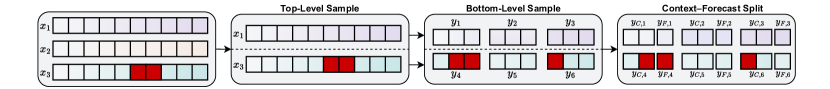
Fig. 1 provides a high-level view of how a single batch is sampled in commonly used forecasting libraries like GluonTS (Alexandrov et al., 2019), and what level of privacy leakage this can cause. Assume we have a dataset of three time series and want to protect any length-2 subsequence (“-event-level privacy” (Kellaris et al., 2014)). First, a subset of time series is selected (“top-level sample”). Then, one or multiple contiguous subsequences are sampled per sequence (“bottom-level sample”). Finally, each subsequence is split into a context window and a ground-truth forecast. As shown in Fig. 1, our length- subsequence may appear in multiple subsequences, with each of its element contributing either to the context or the forecast window. Thus, these elements may leak their information through multiple clipped and noised per-subsequence gradients — either as context via the model’s computation graph or as ground-truth via the loss function.
This risk of multiple leakage is underestimated if we apply privacy guarantees for standard DP-SGD in a black-box manner, and overestimated if we assume that every subsequence always contains every piece of sensitive information (e.g. (Arcolezi et al., 2022)).
Our main contributions are that we, for the first time,
-
•
derive event- and user-level privacy guarantees for bottom-level sampling of contiguous subsequences,
-
•
analyze how the strength of these guarantees can be amplified by top-level sampling,
-
•
and prove how data augmentation can exploit the context–forecast split to further amplify privacy.
Beyond these main contributions, our work demonstrates the usefulness of coupling-based subsampling analysis (Balle et al., 2018; Schuchardt et al., 2024), which has thus far only been applied to unstructured subsampling, in analyzing non-standard, structured subsampling schemes.
2 Related Work
In this section, we discuss some of the most directly related work, and refer the reader to Appendix A for further details.
DP Time Series Release. Koga et al. (2022) and Li et al. (2023) use subsampling to amplify the privacy of differentially private time series release. In particular, Koga et al. (2022) consider a single time series where any individual contributes to a bounded number of steps. They use subsampling in the time domain to reduce the probability of accessing these steps. Note that their sampling distribution ignores temporal structure and yields irregularly sampled time series. Li et al. (2023) combines amplification by subsampling and shuffling on the dataset level, i.e., they only randomize which time series is accessed and not which part of the time series. In general, our goal is training private models rather than publishing sanitized data.
Application of DP-SGD to Time Series. Various works have applied DP-SGD (Mercier et al., 2021; Imtiaz et al., 2020; Arcolezi et al., 2022) or random input perturbations (Li et al., 2019) in specific domains like healthcare data and human mobility. However, they do not tailor their analysis or algorithms to time series data, and instead use DP-SGD or other mechanisms in a black-box manner. Similarly, some works have applied DP-SGD to generative models for time series (Frigerio et al., 2019; Wang et al., 2020a; Torfi et al., 2022) or applied PATE (Papernot et al., 2016) in conjunction with DP-SGD (Lamp et al., 2024). This paper differs from prior work in that we specifically tailor our analysis to the structured nature of time series and the structured sampling of batches in forecasting.
Bi-Level Subsampling for LLMs. Charles et al. (2024) and (Chua et al., 2024) use bi-level subsampling schemes for centralized finetuning of language models on the data of multiple users with multiple sensitive records. However, their privacy analysis only leverages the randomness induced by one of the sampling levels. The other level could equivalently be replaced by a deterministic procedure (see Section A for more details). In comparison, we analyze the interplay of the randomness inherent to both levels. Further note that their analysis considers arbitrary records, and is not tailored to the sequential structure of natural language.
3 Background and Preliminaries
3.1 Differential Privacy
The goal of differential privacy (Dwork, 2006) is to map from a dataset space to an output space while ensuring indistinguishability of any neighboring pair of datasets that differ in one unit of sensitive information (e.g., two sets that differ in one element). In the following, we assume . Differential privacy achieves this goal of indistinguishability via randomization, i.e., mapping to outputs via a random mechanism . The random outputs are considered indistinguishable if the probability of any event only differs by a small factor and constant, i.e., . This is equivalent to bounding the hockey stick divergence of output distributions (Barthe & Olmedo, 2013):
Definition 3.1.
Mechanism is -DP if and only if with
3.2 Private Training and Dominating Pairs
In the case of DP-SGD (Song et al., 2013), the mechanism is a single training step or epoch that maps training samples to updated model weights (for details, see Section 4). A training run is the repeated application of this mechanism. A central notion for determining privacy parameters of such a composed mechanism is that of dominating pairs (Zhu et al., 2022), which fully characterize the tradeoff between and of its component mechanisms.
Definition 3.2.
Distributions are a dominating pair for component mechanism if for all . If the bound holds with equality for all , then are a tight dominating pair.
Tight dominating pairs optimally characterize the trade-off between DP parameters . We will repeatedly show and to be univariate Gaussian mixtures, for which we use the following short-hand (Choquette-Choo et al., 2024).
Definition 3.3.
The mixture-of-Gaussians distribution with means , standard deviation , and weights is .
Given dominating pairs for each component mechanism, one can determine and of the composed mechanism (training run) via privacy accounting methods, such as moments accounting (Abadi et al., 2016) or privacy loss distribution accounting (Meiser & Mohammadi, 2018; Sommer et al., 2019), which we explain in more detail in Section D.3.
3.3 Amplification by Subsampling and Couplings
A key property that enables private training for many iterations with strong privacy guarantees is amplification by subsampling (Kasiviswanathan et al., 2011): Computing gradients for randomly sampled batches strengthens differential privacy (Abadi et al., 2016). More generally, one can use a subsampling scheme that maps from dataset space to a space of batches and an (-DP base mechanism that maps these batches to outputs to construct a more private subsampled mechanism . Balle et al. (2018) propose the use of couplings as a tool for analyzing subsampled mechanisms.
Definition 3.4.
A coupling between distributions of randomly sampled batches is a joint distribution on whose marginals are and .
Intuitively, indicates which batches from the support of correspond to which batches from the support of (for a more thorough introduction, see (Villani, 2009)). Balle et al. (2018) prove that any such coupling yields a bound on the divergence of the subsampled output distributions and . More recently, Schuchardt et al. (2024) have generalized this tool to enable the derivation of dominating pairs for subsampled mechanisms, which we utilize in our proofs and explain in more detail in Section D.1.
3.4 Differential Privacy for Time Series
In the following, we consider the domain of univariate time series of length . We discuss the straight-forward generalization of our results to multivariate time series in Appendix I. The goal of DP time series analysis is to compute statistics for a single series while protecting short contiguous subsequences (“-event-level privacy” (Kellaris et al., 2014)) or all steps to which an individual contributed (“user-level privacy” (Dwork et al., 2010)). For our deep learning context, we define the dataset space to be the powerset and generalize these notions of indistinguishability to datasets as follows:
Definition 3.5.
Datsets and are -event-level neighboring () if they only differ in a single pair of sequences that only differ in a range of indices of length , i.e., for some .
Definition 3.6.
Datsets and are -user-level neighboring () if they only differ in a single pair of sequences that only differ in indices, i.e., .
For example, if our data were the number of patients in hospitals over days, then -event level privacy would protect a patient’s visit to a hospital for up to days while -user-level privacy would also protect multiple shorter visits.111The number of elements in -user-level privacy is often omitted for historical reasons, but still used in deriving privacy guarantees, see, e.g., in Table 1 and Fig. 2 of (Mao et al., 2024). Depending on the domain, these relations can be made more precise by constraining the magnitude of change (e.g., (Koga et al., 2022)). For instance, an individual can only change the number of patients on a day by . We refer to this as -event and -user-level privacy.
Definition 3.7.
Consider datasets or that differ in sequences . If , then we refer to them as -event and -user-level neighboring ( and ) , respectively.
4 Deep Differentially Private Forecasting
Now that we have the language to formally reason about privacy, let us turn to our original goal of training forecasting models. Algorithm 1 describes the use of top- and bottom-level sampling (recall Fig. 1), which we instantiate shortly. Given a dataset of sequences , we sample a subset of sequences, and then independently sample subsequences from of each them. All subsequences are then aggregated into a single batch . The size of the top-level sample is chosen such that we (up to modulo division) attain a batch size of . Algorithm 2 formalizes the splitting of each subsequence into a context and ground-truth forecast window. Unlike in standard training, we clip the gradient of the corresponding loss and add calibrated Gaussian noise with covariance matrix . This makes the training step differentially private under insertion/removal of a batch element (Abadi et al., 2016).
Contribution. Importantly, we neither claim the batching procedure nor the noisy training step to be novel in isolation. Our novel contribution lies in analyzing the interesting and non-trivial way in which the components of the batching procedure interact to amplify the privacy of training steps.
Simplifying assumptions. For the sake of exposition and to simplify notation, we assume that and focus on -event-level privacy. In Appendix I, we discuss how to easily generalize our guarantees to -event and -user-level privacy with arbitrary , as well as variable-length and multivariate time series.
4.1 Bottom-Level Subsampling
Let us begin by focusing on the amplification attained via bottom-level sampling of temporally contiguous subsequences. To this end, we assume that the top-level sampling procedure simply iterates deterministically over our dataset and yields sequences per batch (see Algorithm 3). As our bottom-level scheme, we use Algorithm 4, which samples subsequences per sequence with replacement to achieve a fixed batch size of . In Section E.2, we additionally consider Poisson sampling, which independently includes each element at a constant rate. In forecasting frameworks, these methods are also referred to as number of instances sampling and uniform split sampling, respectively (Alexandrov et al., 2019). In the following, mechanism refers to a single epoch with top-level iteration and bottom-level sampling with replacement.
Effect of Number of Subsequences . Before we proceed to deriving amplification guarantees, note that bi-level subsampling introduces an additional degree of freedom not present in DP-SGD for unstructured data: A batch of size can be composed of many subsequences from few sequences ( large) or few subsequences from many sequences ( small). Intuitively, the latter should be more private, because there are fewer chances to access sensitive information from any specific sequence . In fact, we can prove the correctness of this intuition via stochastic dominance of amplification bounds (see Section E.3):
Theorem 4.1.
Let , be a tight dominating pair of epoch for bottom-level Poisson sampling or sampling with replacement and (expected) subsequences. Then is minimized by for all .
Guarantees for Optimal . Based on this result, let us begin by focusing on the case that minimizes per-epoch privacy leakage. Because we consider subsequences of length , even a single sensitive element of a sequence can contribute to different subsequences at different positions. Since we deterministically iterate over our dataset, these subsequences can contribute to exactly one training step per epoch. The resultant privacy is tightly bounded by the following result (proof in Appendix E).
Theorem 4.2.
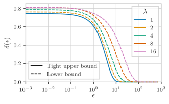
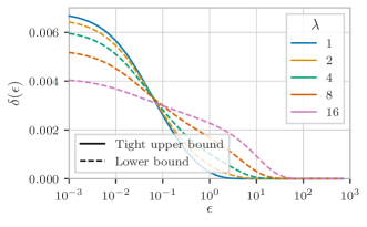
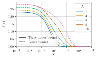
Consider the number of sampled subsequences , and let be the probability of sampling a subsequence containing any specific element. Define with means and weights . Further, define per-epoch privacy profile . Then,
In Section E.1.5, we discuss the tight dominating pairs corresponding to this bound. Intuitively, as decreases, converges to and the hockey stick divergence decreases, i.e., our mechanism becomes more private.
Other Guarantees. In Appendix E, we derive tight dominating pairs for Poisson sampling and , as well as dominating pairs for sampling with replacement and . The special case of , is equivalent to sampling from a set in which elements are substituted, i.e., subsampled group privacy (Ganesh, 2024; Schuchardt et al., 2024; Jiang et al., 2025). Thus far, tight dominating pairs have only been known for group insertion/removal, i.e., these guarantees are of interest beyond forecasting.
Epoch Privacy vs Length. Despite the optimality guarantee from Theorem 4.1, we need to consider that sampling few subsequences ( small) means that more sequences contribute to a batch ( large). We thus need more epochs for the same number of training steps, and each epoch has the potential of leaking private information. In Section 5, we will demonstrate numerically that composing many short, more private epochs () nevertheless offers stronger privacy for the same number of training steps. As baselines for this experiment, we will use the following optimistic lower bounds (proof in Section E.1.4):
Theorem 4.3.
Consider the number of subsequences , and let . Define with means and weights with and . Further, define per-epoch privacy profile . Then,
Intuitively, each mixture mean corresponds to the event that subsequences with information of a specific individual are sampled, i.e., more information is leaked.
4.2 Top-Level Subsampling
Next, let us explore how randomizing which sequences contribute to a batch can further amplify privacy. For this, we use Algorithm 5, which samples without replacement. This will eliminate the chance that any particular sequence can have its information leaked through more than subsequences per batch. From here on, mechanism refers to a single training step using top-level sampling without replacement and bottom-level sampling with replacement.
Theorem 4.4.
Consider the number of subsequences and batch size . Let and let be the probability of sampling any specific sequence. Define with and . Then, per-step privacy profile fulfills
Intuitively, removes probability mass from the mixture component that indicates some level of privacy leakage, and transfers it to the component that indicates zero leakage.
Other guarantees. In Appendix F, we additionally derive dominating pairs for when using bottom-level sampling with replacement or Poisson sampling. There, still has a similar effect of attenuating privacy leakage.
Step- vs Epoch-Level Accounting. While Theorem 4.4 shows that top-level sampling amplifies privacy, it yields bounds for each training step instead of each epoch (cf. Theorem 4.2). We need to self-compose these bounds times to obtain epoch-level guarantees (see Algorithm 1). In Section 5 we confirm that the resulting privacy guarantees can nevertheless be stronger than our original epoch-level guarantee. This observation is consistent with works on DP-SGD for unstructured data that self-compose subsampled mechanisms instead of deterministically iterating over datasets (e.g. (Abadi et al., 2016)).
Choice of . As before, we can ask ourselves which number of subsequences per sequence we should choose. In bi-level subsampling, there is a more intricate trade-off, because increasing decreases , i.e., strengthens top-level amplification, but weakens bottom-level amplification (recall Theorem 4.1). In Section 5, we demonstrate numerically that is still preferable under composition. As fair baselines for this experiment, we use optimistic lower bounds for that we derive in Section F.4.
4.3 Context–Forecast Split
We have already successfully analyzed how top- and bottom-level subsampling interact to amplify the privacy of clipped and noised gradients . However, we can use yet another level of forecasting-specific randomness — if we assume that an individual can change each value of a series by at most , i.e., we assume -event or -user-level privacy (Definition 3.7). We propose to augment the context and forecast window with Gaussian noise , :
| (1) |
Unlike the input perturbations from (Arcolezi et al., 2022) which are an offline pre-processing that privatizes the dataset, Eq. 1 is an online data augmentation that serves as an integral part of the (now continuous) subsampling procedure. In the following, let refer to a single training step when combining top-level sampling without replacement, bottom-level sampling with replacement, and Eq. 1.
Amplification by Data Augmentation. Intuitively, any element can only contribute to gradient either via context or via ground-truth forecast . Even if this element changes by , there is a chance that we sample the same value after adding Gaussian noise, i.e., have zero leakage. In Appendix G, we use conditional couplings in conjunction with the maximal couplings originally used for subsampling analysis by Balle et al. (2018) to formalize “sampling the same value” and prove amplification for arbitrary . The following result shows the special case where the noise scale for the context and forecast window is identical (for the general case, see Theorem G.1).
Theorem 4.5.
Consider , batch size , as well as context and forecast standard deviations with . Let and . Define with means and weights , with and
with total variation distance . Then, fulfills
Intuitively, this shows that Gaussian data augmentation has a similar effect to subsampling in that it shifts probability mass to the mixture component that indicates zero leakage.
Amplification by Label Perturbation. An interesting special case is , where privacy is only further amplified when sensitive information appears as a ground-truth forecast, i.e., we are in the “label privacy” (Chaudhuri & Hsu, 2011) setting. A standard technique for deep learning with label privacy is using random label perturbations as an offline pre-processing step (Ghazi et al., 2021). Our results in Appendix G show for the first time how online label perturbations can amplify privacy in settings where we randomly switch between feature- and label-privacy, such as self-supervised (pre-)training of sequence models.
4.4 Additional Inference-Time Privacy
Like other works on DP-SGD, we focus on ensuring privacy of parameters to guarantee that information from any training sequence does not leak when releasing the model or forecasts for other sequences . In Appendix H, we additionally explore the use of input perturbations in combination with subsampling and imputation to ensure privacy for elements of when releasing forecast .
4.5 Limitations and Future Work
Since we are first to analyze forecasting-specific subsampling, there are still opportunities for improvement, namely by further tightening our guarantees for (1) bottom-level sampling with replacement and , (2) top-level sampling without replacement and , and potentially (3) amplification by augmentation. While we numerically investigate the discussed trade-offs in parameterizing our subsampling scheme, future work may also want to investigate them analytically, e.g., via central limit theorems (Sommer et al., 2019; Dong et al., 2022). Finally, the connection between event and -event-level privacy and token- or sentence-level private language modeling (Hu et al., 2024) (i.e., autoregressive probabilistic forecasting for discrete-valued time series) is immediate and should be explored in future work.
5 Experimental Evaluation
We already achieved our primary objective of deriving time-series-specific subsampling guarantees for DP-SGD adapted to forecasting. Our main goal for this section is to investigate the trade-offs we discovered in discussing these guarantees. In addition, we train common probabilistic forecasting architectures on standard datasets to verify the feasibility of training deep differentially private forecasting models while retaining meaningful utility. The full experimental setup is described in Appendix B.
5.1 Trade-Offs in Structured Subsampling
For the following experiments, we assume that we have sequences, batch size , and noise scale . We further assume , so that the chance of bottom-level sampling a subsequence containing any specific element is when choosing as the number of subsequences. In Section C.1, we repeat all experiments with a wider range of parameters. All results are consistent with the ones shown here.
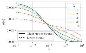
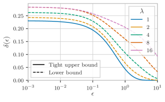
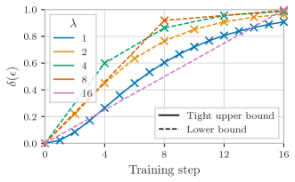
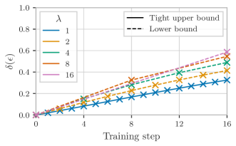
Number of Subsequences . Let us begin with a trade-off inherent to bi-level subsampling: We can achieve the same batch size with different , each leading to different top- and bottom-level amplification. We claim that (i.e., maximum bottom-level amplification) is preferable. For a fair comparison, we compare our provably tight guarantee for (Theorem 4.4) with optimistic lower bounds for (Theorem F.7) instead of our sound upper bounds (Theorem F.1), i.e., we make the competitors stronger. As shown in Fig. 4(a), only has smaller for when considering a single training step. However, after -fold composition, achieves smaller even in (see Fig. 4(b)). Our explanation is that results in larger for large , i.e., is more likely to have a large privacy loss. Because the privacy loss of a composed mechanism is the sum of component privacy losses (Sommer et al., 2019), this is problematic when performing multiple training steps. We shall thus later use for training.
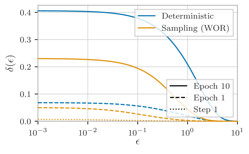
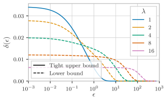
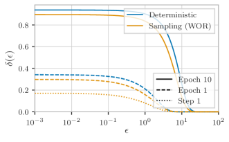
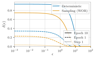
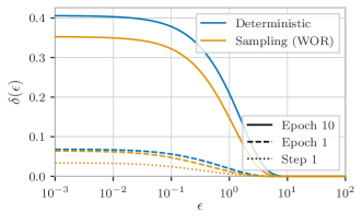
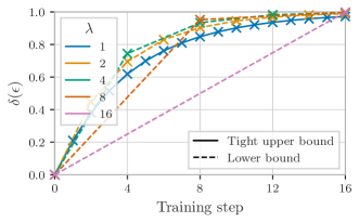
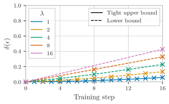
Step- vs Epoch-Level Accounting. Next, we show the benefit of top-level sampling sequences (Theorem 4.4) instead of deterministically iterating over them (Theorem 4.2), even though we risk privacy leakage at every training step. For our parameterization and , top-level sampling with replacement requires compositions per epoch. As shown in Fig. 2, the resultant epoch-level profile is nevertheless smaller, and remains so after epochs. This is consistent with any work on DP-SGD (e.g., (Abadi et al., 2016)) that uses subsampling instead of deterministic iteration.
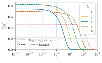
Epoch Privacy vs Length. In Section C.1.4 we additionally explore the fact that, if we wanted to use deterministic top-level iteration, the number of subsequences would affect epoch length. As expected, we observe that composing many private mechanisms () is preferable to composing few much less private mechanisms () when considering a fixed number of training steps.
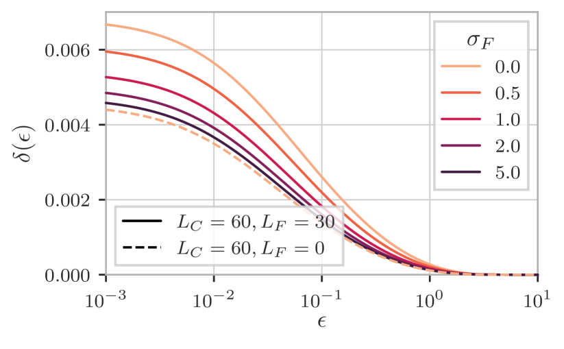
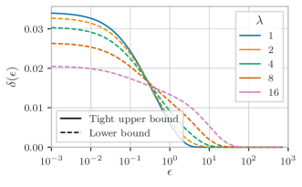
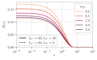
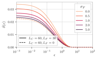
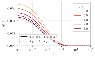
Amplification by Label Perturbation. Finally, because the way in which adding Gaussian noise to the context and/or forecast window amplifies privacy (Theorem G.1) may be somewhat opaque, let us consider top-level sampling without replacement, bottom-level sampling with replacement, , , and varying label noise standard deviations . As shown in Fig. 3, increasing has the same effect as letting the forecast length go to zero, i.e., eliminates the risk of leaking private information if it appears in the forecast window. Of course, this data augmentation will have an effect on model utility, which we investigate shortly.
5.2 Application to Probabilistic Forecasting
While the contribution of our work lies in formally analyzing the privacy of DP-SGD adapted to forecasting, training models with this algorithm can serve as a sanity-check to verify that the guarantees are sufficiently strong to retain meaningful utility under non-trivial privacy budgets.
| Model | ||||
|---|---|---|---|---|
| SimpleFF | ||||
| DeepAR | ||||
| iTransf. | ||||
| DLinear | ||||
| Seasonal | ||||
| AutoETS |
Datasets, Models, and Metrics. We consider three standard benchmarks: traffic, electricity, and solar_10_minutes as used in (Lai et al., 2018). We further consider four common architectures: A two-layer feed-forward neural network (“SimpleFeedForward”), a recurrent neural network (“DeepAR” (Salinas et al., 2020)), an encoder-only transformer (“iTransformer” (Liu et al., 2024)), and a refined feed-forward network proposed to compete with attention-based models (“DLinear” (Zeng et al., 2023)). We let these architectures parameterize elementwise -distributions to obtain probabilistic forecasts. We measure the quality of these probabilistic forecasts using continuous ranked probability scores (CRPS), which we approximate via mean weighted quantile losses (details in Section B.3). As a reference for what constitutes “meaningful utility”, we compare against seasonal naïve forecasting and exponential smoothing (“AutoETS”) without introducing any noise. All experiments are repeated with random seeds.
Event-Level Privacy. Table 1 shows CRPS of all models on the traffic test set when setting , and training on the training set until reaching a pre-specified with -event-level privacy. For the other datasets and standard deviations, see Section C.2.1. The column indicates non-DP training. As can be seen, models can retain much of their utility and outperform the baselines, even for which is generally considered a small privacy budget (Ponomareva et al., 2023). For instance, the average CRPS of DeepAR on the traffic dataset is with non-DP training and for . Note that, since all models are trained using our tight privacy analysis, which specific model performs best on which specific dataset is orthogonal to our contribution.
Other results. In Section C.2.2 we additionally train with -event and -user privacy. In Section C.2.3, we demonstrate that label perturbations can offer an improved privacy–utility trade-off. All results confirm that our guarantees for DP-SGD adapted to forecasting are strong enough to enable provably private training while retaining utility.
6 Conclusion
In this work, we answer the question how DP-SGD can be adapted to time series forecasting while accounting for domain- and task-specific aspects. We derive privacy amplification guarantees for sampling contiguous subsequences and for combining this bottom-level sampling with top-level sampling of sequences, and additionally prove that partitioning subsequences into context and ground-truth forecasts enables privacy amplification by data augmentation. We further identify multiple trade-offs inherent to bi-level subsampling which we investigate theoretically and/or numerically. Finally, we confirm empirically that it is feasible to train differentially private forecasting models while retaining meaningful utility. Adapting our results to natural language represents a promising direction for future work towards trustworthy machine learning on structured data.
Acknowledgements
We would like to thank Dominik Fuchsgruber, Jonas Dornbusch, Marcel Kollovieh, and Leo Schwinn for proofreading the manuscript. We are also grateful to Marcel Kollovieh, Kashif Rasul, and Marin Biloš for providing valuable insights into practical aspects of training forecasting models.
Impact Statement
This work is specifically aimed at mitigating negative societal impact of machine learning by provably ensuring that forecasts made by a model trained on sensitive data does not allow for any form of membership inference or reconstruction attack. As such, even though there are many potential societal consequences of our work, we do not feel that any of them must be specifically highlighted here.
References
- Abadi et al. (2016) Abadi, M., Chu, A., Goodfellow, I., McMahan, H. B., Mironov, I., Talwar, K., and Zhang, L. Deep learning with differential privacy. In Proceedings of the 2016 ACM SIGSAC conference on computer and communications security, pp. 308–318, 2016.
- Alexandrov et al. (2019) Alexandrov, A., Benidis, K., Bohlke-Schneider, M., Flunkert, V., Gasthaus, J., Januschowski, T., Maddix, D. C., Rangapuram, S., Salinas, D., Schulz, J., et al. Gluonts: Probabilistic time series models in python. arXiv preprint arXiv:1906.05264, 2019.
- Arcolezi et al. (2022) Arcolezi, H. H., Couchot, J.-F., Renaud, D., Al Bouna, B., and Xiao, X. Differentially private multivariate time series forecasting of aggregated human mobility with deep learning: Input or gradient perturbation? Neural Computing and Applications, 34(16):13355–13369, 2022.
- Balle & Wang (2018) Balle, B. and Wang, Y.-X. Improving the gaussian mechanism for differential privacy: Analytical calibration and optimal denoising. In International Conference on Machine Learning, pp. 394–403, 2018.
- Balle et al. (2018) Balle, B., Barthe, G., and Gaboardi, M. Privacy amplification by subsampling: Tight analyses via couplings and divergences. Advances in neural information processing systems, 31, 2018.
- Balle et al. (2020) Balle, B., Barthe, G., and Gaboardi, M. Privacy profiles and amplification by subsampling. Journal of Privacy and Confidentiality, 10(1), 2020.
- Barthe & Olmedo (2013) Barthe, G. and Olmedo, F. Beyond differential privacy: Composition theorems and relational logic for f-divergences between probabilistic programs. In Fomin, F. V., Freivalds, R., Kwiatkowska, M., and Peleg, D. (eds.), Automata, Languages, and Programming, pp. 49–60, 2013.
- Carranza et al. (2023) Carranza, A. G., Farahani, R., Ponomareva, N., Kurakin, A., Jagielski, M., and Nasr, M. Synthetic query generation for privacy-preserving deep retrieval systems using differentially private language models. arXiv preprint arXiv:2305.05973, 2023.
- Charles et al. (2024) Charles, Z., Ganesh, A., McKenna, R., McMahan, H. B., Mitchell, N., Pillutla, K., and Rush, K. Fine-tuning large language models with user-level differential privacy. arXiv preprint arXiv:2407.07737, 2024.
- Chaudhuri & Hsu (2011) Chaudhuri, K. and Hsu, D. Sample complexity bounds for differentially private learning. In Proceedings of the 24th Annual Conference on Learning Theory, pp. 155–186, 2011.
- Chen et al. (2001) Chen, C., Petty, K., Skabardonis, A., Varaiya, P., and Jia, Z. Freeway performance measurement system: mining loop detector data. Transportation research record, 1748(1):96–102, 2001.
- Chen et al. (2024) Chen, Y., Biloš, M., Mittal, S., Deng, W., Rasul, K., and Schneider, A. Recurrent interpolants for probabilistic time series prediction. In NeurIPS 2024 Third Table Representation Learning Workshop, 2024. URL https://openreview.net/forum?id=gYNpjdaN5j.
- Choquette-Choo et al. (2024) Choquette-Choo, C. A., Ganesh, A., Steinke, T., and Thakurta, A. G. Privacy amplification for matrix mechanisms. In International Conference on Learning Representations, 2024.
- Chua et al. (2024) Chua, L., Ghazi, B., Huang, Y., Kamath, P., Kumar, R., Liu, D., Manurangsi, P., Sinha, A., and Zhang, C. Mind the privacy unit! user-level differential privacy for language model fine-tuning. arXiv preprint arXiv:2406.14322, 2024.
- Den Hollander (2012) Den Hollander, F. Probability theory: The coupling method. Lecture notes available online (http://websites. math. leidenuniv. nl/probability/lecturenotes/CouplingLectures. pdf), 2012.
- Dong et al. (2022) Dong, J., Roth, A., and Su, W. J. Gaussian differential privacy. Journal of the Royal Statistical Society Series B: Statistical Methodology, 84(1):3–37, 2022.
- Doroshenko et al. (2022) Doroshenko, V., Ghazi, B., Kamath, P., Kumar, R., and Manurangsi, P. Connect the dots: Tighter discrete approximations of privacy loss distributions. Proceedings on Privacy Enhancing Technologies, 2022.
- Dwork (2006) Dwork, C. Differential privacy. In Automata, Languages and Programming: 33rd International Colloquium, ICALP 2006, Venice, Italy, July 10-14, 2006, Proceedings, Part II 33, pp. 1–12. Springer, 2006.
- Dwork & Rothblum (2016) Dwork, C. and Rothblum, G. N. Concentrated differential privacy. arXiv preprint arXiv:1603.01887, 2016.
- Dwork et al. (2010) Dwork, C., Naor, M., Pitassi, T., and Rothblum, G. N. Differential privacy under continual observation. In Proceedings of the Forty-Second ACM Symposium on Theory of Computing, STOC ’10, pp. 715–724, 2010.
- El Ouadrhiri & Abdelhadi (2022) El Ouadrhiri, A. and Abdelhadi, A. Differential privacy for deep and federated learning: A survey. IEEE access, 10:22359–22380, 2022.
- Falcetta & Roveri (2022) Falcetta, A. and Roveri, M. Privacy-preserving time series prediction with temporal convolutional neural networks. In 2022 International Joint Conference on Neural Networks (IJCNN), pp. 1–8, 2022.
- Fan & Xiong (2014) Fan, L. and Xiong, L. An adaptive approach to real-time aggregate monitoring with differential privacy. IEEE Transactions on Knowledge and Data Engineering, 26(9):2094–2106, 2014.
- Feldman et al. (2018) Feldman, V., Mironov, I., Talwar, K., and Thakurta, A. Privacy amplification by iteration. In 2018 IEEE 59th Annual Symposium on Foundations of Computer Science (FOCS), pp. 521–532. IEEE, 2018.
- Fioretto & Van Hentenryck (2019) Fioretto, F. and Van Hentenryck, P. Optstream: Releasing time series privately. Journal of Artificial Intelligence Research, 65:423–456, 2019.
- Frigerio et al. (2019) Frigerio, L., de Oliveira, A. S., Gomez, L., and Duverger, P. Differentially private generative adversarial networks for time series, continuous, and discrete open data. In ICT Systems Security and Privacy Protection: 34th IFIP TC 11 International Conference, SEC 2019, Lisbon, Portugal, June 25-27, 2019, Proceedings 34, pp. 151–164, 2019.
- Ganesh (2024) Ganesh, A. Tight group-level dp guarantees for dp-sgd with sampling via mixture of gaussians mechanisms. arXiv preprint arXiv:2401.10294, 2024.
- Garza et al. (2022) Garza, A., Canseco, M., Challú, C., and Olivares, K. StatsForecast: Lightning fast forecasting with statistical and econometric models. PyCon Salt Lake City, Utah, US 2022, 2022. URL https://github.com/Nixtla/statsforecast.
- Ghazi et al. (2021) Ghazi, B., Golowich, N., Kumar, R., Manurangsi, P., and Zhang, C. Deep learning with label differential privacy. Advances in neural information processing systems, 34:27131–27145, 2021.
- Giannotti & Pedreschi (2008) Giannotti, F. and Pedreschi, D. Mobility, data mining and privacy: Geographic knowledge discovery. Springer Science & Business Media, 2008. ISBN 9783540751762.
- Gneiting & Raftery (2007) Gneiting, T. and Raftery, A. E. Strictly proper scoring rules, prediction, and estimation. Journal of the American statistical Association, 102(477):359–378, 2007.
- Google Differential Privacy Team (2024) Google Differential Privacy Team. Privacy loss distributions. https://raw.githubusercontent.com/google/differential-privacy/main/common_docs/Privacy_Loss_Distributions.pdf, 2024. Accessed May 22, 2024.
- Gopi et al. (2021) Gopi, S., Lee, Y. T., and Wutschitz, L. Numerical composition of differential privacy. Advances in Neural Information Processing Systems, 34:11631–11642, 2021.
- Hu et al. (2024) Hu, L., Habernal, I., Shen, L., and Wang, D. Differentially private natural language models: Recent advances and future directions. In Graham, Y. and Purver, M. (eds.), Findings of the Association for Computational Linguistics: EACL 2024, pp. 478–499, 2024.
- Imtiaz et al. (2020) Imtiaz, S., Horchidan, S.-F., Abbas, Z., Arsalan, M., Chaudhry, H. N., and Vlassov, V. Privacy preserving time-series forecasting of user health data streams. In 2020 IEEE International Conference on Big Data (Big Data), pp. 3428–3437, 2020.
- Januschowski et al. (2020) Januschowski, T., Gasthaus, J., Wang, Y., Salinas, D., Flunkert, V., Bohlke-Schneider, M., and Callot, L. Criteria for classifying forecasting methods. International Journal of Forecasting, 36(1):167–177, 2020.
- Jiang et al. (2025) Jiang, Y., Luo, X., Yang, Y., and Xiao, X. Calibrating noise for group privacy in subsampled mechanisms. In International Conference on Very Large Data Bases, 2025.
- Kasiviswanathan et al. (2011) Kasiviswanathan, S. P., Lee, H. K., Nissim, K., Raskhodnikova, S., and Smith, A. What can we learn privately? SIAM Journal on Computing, 40(3):793–826, 2011.
- Katsomallos et al. (2019) Katsomallos, M., Tzompanaki, K., and Kotzinos, D. Privacy, space and time: A survey on privacy-preserving continuous data publishing. Journal of Spatial Information Science, 2019(19):57–103, 2019.
- Kellaris et al. (2014) Kellaris, G., Papadopoulos, S., Xiao, X., and Papadias, D. Differentially private event sequences over infinite streams. Proc. VLDB Endow., 7(12):1155–1166, August 2014.
- Koga et al. (2022) Koga, T., Meehan, C., and Chaudhuri, K. Privacy amplification by subsampling in time domain. In International Conference on Artificial Intelligence and Statistics, pp. 4055–4069. PMLR, 2022.
- Kollovieh et al. (2024) Kollovieh, M., Ansari, A. F., Bohlke-Schneider, M., Zschiegner, J., Wang, H., and Wang, Y. B. Predict, refine, synthesize: Self-guiding diffusion models for probabilistic time series forecasting. Advances in Neural Information Processing Systems, 36, 2024.
- Koskela et al. (2020) Koskela, A., Jälkö, J., and Honkela, A. Computing tight differential privacy guarantees using fft. In International Conference on Artificial Intelligence and Statistics, pp. 2560–2569, 2020.
- Lai et al. (2018) Lai, G., Chang, W.-C., Yang, Y., and Liu, H. Modeling long- and short-term temporal patterns with deep neural networks. In The 41st International ACM SIGIR Conference on Research & Development in Information Retrieval, SIGIR ’18, pp. 95–104, 2018. ISBN 9781450356572.
- Lamp et al. (2024) Lamp, J., Derdzinski, M., Hannemann, C., Van der Linden, J., Feng, L., Wang, T., and Evans, D. Glucosynth: Generating differentially-private synthetic glucose traces. Advances in Neural Information Processing Systems, 36, 2024.
- Lana et al. (2018) Lana, I., Del Ser, J., Velez, M., and Vlahogianni, E. I. Road traffic forecasting: Recent advances and new challenges. IEEE Intelligent Transportation Systems Magazine, 10(2):93–109, 2018.
- Lebeda et al. (2024) Lebeda, C. J., Regehr, M., Kamath, G., and Steinke, T. Avoiding pitfalls for privacy accounting of subsampled mechanisms under composition. arXiv preprint arXiv:2405.20769, 2024.
- Lee & Søgaard (2023) Lee, S. and Søgaard, A. Private meeting summarization without performance loss. In Proceedings of the 46th International ACM SIGIR Conference on Research and Development in Information Retrieval, pp. 2282–2286, 2023.
- Li et al. (2015) Li, H., Xiong, L., Jiang, X., and Liu, J. Differentially private histogram publication for dynamic datasets: an adaptive sampling approach. In Proceedings of the 24th ACM International on Conference on Information and Knowledge Management, CIKM ’15, pp. 1001–1010, 2015.
- Li et al. (2019) Li, X., Li, Y., Yang, H., Yang, L., and Liu, X.-Y. Dp-lstm: Differential privacy-inspired lstm for stock prediction using financial news. arXiv preprint arXiv:1912.10806, 2019.
- Li et al. (2023) Li, X., Cao, Y., and Yoshikawa, M. Locally private streaming data release with shuffling and subsampling. In 2023 IEEE 39th International Conference on Data Engineering Workshops (ICDEW), pp. 125–131, 2023.
- Liu et al. (2021) Liu, B., Ding, M., Shaham, S., Rahayu, W., Farokhi, F., and Lin, Z. When machine learning meets privacy: A survey and outlook. ACM Computing Surveys (CSUR), 54(2):1–36, 2021.
- Liu et al. (2024) Liu, Y., Hu, T., Zhang, H., Wu, H., Wang, S., Ma, L., and Long, M. itransformer: Inverted transformers are effective for time series forecasting. In The Twelfth International Conference on Learning Representations, 2024.
- Mao et al. (2024) Mao, Y., Ye, Q., Wang, Q., and Hu, H. Differential privacy for time series: A survey. IEEE Data Eng. Bull., 47(2):67–92, 2024.
- McMahan et al. (2017) McMahan, H. B., Ramage, D., Talwar, K., and Zhang, L. Learning differentially private recurrent language models. arXiv preprint arXiv:1710.06963, 2017.
- McSherry (2009) McSherry, F. D. Privacy integrated queries: an extensible platform for privacy-preserving data analysis. In Proceedings of the 2009 ACM SIGMOD International Conference on Management of data, pp. 19–30, 2009.
- Meiser & Mohammadi (2018) Meiser, S. and Mohammadi, E. Tight on budget? tight bounds for r-fold approximate differential privacy. In Proceedings of the ACM SIGSAC Conference on Computer and Communications Security, pp. 247–264, 2018.
- Mercier et al. (2021) Mercier, D., Lucieri, A., Munir, M., Dengel, A., and Ahmed, S. Evaluating privacy-preserving machine learning in critical infrastructures: A case study on time-series classification. IEEE Transactions on Industrial Informatics, 18(11):7834–7842, 2021.
- Mironov (2017) Mironov, I. Rényi differential privacy. In IEEE 30th computer security foundations symposium (CSF), pp. 263–275, 2017.
- Mueller et al. (2022) Mueller, T. T., Usynin, D., Paetzold, J. C., Rueckert, D., and Kaissis, G. Sok: Differential privacy on graph-structured data. arXiv preprint arXiv:2203.09205, 2022.
- Olatunji et al. (2021) Olatunji, I. E., Funke, T., and Khosla, M. Releasing graph neural networks with differential privacy guarantees. arXiv preprint arXiv:2109.08907, 2021.
- Pan et al. (2024) Pan, K., Ong, Y.-S., Gong, M., Li, H., Qin, A. K., and Gao, Y. Differential privacy in deep learning: A literature survey. Neurocomputing, pp. 127663, 2024.
- Papernot et al. (2016) Papernot, N., Abadi, M., Erlingsson, U., Goodfellow, I., and Talwar, K. Semi-supervised knowledge transfer for deep learning from private training data. arXiv preprint arXiv:1610.05755, 2016.
- Ponomareva et al. (2023) Ponomareva, N., Hazimeh, H., Kurakin, A., Xu, Z., Denison, C., McMahan, H. B., Vassilvitskii, S., Chien, S., and Thakurta, A. G. How to dp-fy ml: A practical guide to machine learning with differential privacy. Journal of Artificial Intelligence Research, 77:1113–1201, 2023.
- Ramaswamy et al. (2020) Ramaswamy, S., Thakkar, O., Mathews, R., Andrew, G., McMahan, H. B., and Beaufays, F. Training production language models without memorizing user data. arXiv preprint arXiv:2009.10031, 2020.
- Rasul et al. (2021) Rasul, K., Sheikh, A.-S., Schuster, I., Bergmann, U. M., and Vollgraf, R. Multivariate probabilistic time series forecasting via conditioned normalizing flows. In International Conference on Learning Representations, 2021.
- Rigaki & Garcia (2023) Rigaki, M. and Garcia, S. A survey of privacy attacks in machine learning. ACM Computing Surveys, 56(4):1–34, 2023.
- Roch (2024) Roch, S. Modern Discrete Probability: An Essential Toolkit. Cambridge Series in Statistical and Probabilistic Mathematics. Cambridge University Press, 2024. doi: 10.1017/9781009305129.
- Salinas et al. (2020) Salinas, D., Flunkert, V., Gasthaus, J., and Januschowski, T. Deepar: Probabilistic forecasting with autoregressive recurrent networks. International journal of forecasting, 36(3):1181–1191, 2020.
- Schuchardt et al. (2024) Schuchardt, J., Stoian, M., Kosmala, A., and Günnemann, S. Unified mechanism-specific amplification by subsampling and group privacy amplification. In The Thirty-eighth Annual Conference on Neural Information Processing Systems, 2024.
- Shchur et al. (2023) Shchur, O., Turkmen, A. C., Erickson, N., Shen, H., Shirkov, A., Hu, T., and Wang, B. Autogluon–timeseries: Automl for probabilistic time series forecasting. In International Conference on Automated Machine Learning, pp. 9–1. PMLR, 2023.
- Shi et al. (2011) Shi, E., Chan, H., Rieffel, E., Chow, R., and Song, D. Privacy-preserving aggregation of time-series data. In Annual Network & Distributed System Security Symposium (NDSS). Internet Society., 2011.
- Sommer et al. (2019) Sommer, D. M., Meiser, S., and Mohammadi, E. Privacy loss classes: The central limit theorem in differential privacy. Proceedings on Privacy Enhancing Technologies, 2019(2):245–269, 2019.
- Song et al. (2013) Song, S., Chaudhuri, K., and Sarwate, A. D. Stochastic gradient descent with differentially private updates. In IEEE global conference on signal and information processing, pp. 245–248, 2013.
- Torfi et al. (2022) Torfi, A., Fox, E. A., and Reddy, C. K. Differentially private synthetic medical data generation using convolutional gans. Information Sciences, 586:485–500, 2022.
- Villani (2009) Villani, C. Optimal Transport. Springer Berlin Heidelberg, 2009. ISBN 9783540710509.
- Wang et al. (2016) Wang, Q., Zhang, Y., Lu, X., Wang, Z., Qin, Z., and Ren, K. Rescuedp: Real-time spatio-temporal crowd-sourced data publishing with differential privacy. In IEEE INFOCOM 2016 - The 35th Annual IEEE International Conference on Computer Communications, pp. 1–9, 2016.
- Wang et al. (2020a) Wang, S., Rudolph, C., Nepal, S., Grobler, M., and Chen, S. Part-gan: Privacy-preserving time-series sharing. In Artificial Neural Networks and Machine Learning–ICANN 2020: 29th International Conference on Artificial Neural Networks, Bratislava, Slovakia, September 15–18, 2020, Proceedings, Part I 29, pp. 578–593. Springer, 2020a.
- Wang et al. (2019) Wang, Y.-X., Balle, B., and Kasiviswanathan, S. P. Subsampled rényi differential privacy and analytical moments accountant. In The 22nd International Conference on Artificial Intelligence and Statistics, pp. 1226–1235, 2019.
- Wang et al. (2020b) Wang, Z., Liu, W., Pang, X., Ren, J., Liu, Z., and Chen, Y. Towards pattern-aware privacy-preserving real-time data collection. In IEEE INFOCOM 2020 - IEEE Conference on Computer Communications, pp. 109–118, 2020b.
- Wunderlich et al. (2022) Wunderlich, D., Bernau, D., Aldà, F., Parra-Arnau, J., and Strufe, T. On the privacy–utility trade-off in differentially private hierarchical text classification. Applied Sciences, 12(21):11177, 2022.
- Ye & Shokri (2022) Ye, J. and Shokri, R. Differentially private learning needs hidden state (or much faster convergence). Advances in Neural Information Processing Systems, 35:703–715, 2022.
- Yousefpour et al. (2021) Yousefpour, A., Shilov, I., Sablayrolles, A., Testuggine, D., Prasad, K., Malek, M., Nguyen, J., Ghosh, S., Bharadwaj, A., Zhao, J., Cormode, G., and Mironov, I. Opacus: User-friendly differential privacy library in PyTorch. arXiv preprint arXiv:2109.12298, 2021.
- Yue et al. (2022) Yue, X., Inan, H. A., Li, X., Kumar, G., McAnallen, J., Shajari, H., Sun, H., Levitan, D., and Sim, R. Synthetic text generation with differential privacy: A simple and practical recipe. arXiv preprint arXiv:2210.14348, 2022.
- Yue et al. (2021) Yue, Z., Ding, S., Zhao, L., Zhang, Y., Cao, Z., Tanveer, M., Jolfaei, A., and Zheng, X. Privacy-preserving time-series medical images analysis using a hybrid deep learning framework. ACM Trans. Internet Technol., 21(3), June 2021. ISSN 1533-5399.
- Zeng et al. (2023) Zeng, A., Chen, M., Zhang, L., and Xu, Q. Are transformers effective for time series forecasting? In Proceedings of the AAAI conference on artificial intelligence, volume 37, pp. 11121–11128, 2023.
- Zhang et al. (2017) Zhang, J., Liang, X., Zhang, Z., He, S., and Shi, Z. Re-dpoctor: Real-time health data releasing with w-day differential privacy. In GLOBECOM 2017 - 2017 IEEE Global Communications Conference, pp. 1–6, 2017.
- Zhang et al. (2022) Zhang, X., Khalili, M. M., and Liu, M. Differentially private real-time release of sequential data. ACM Transactions on Privacy and Security, 26(1):1–29, 2022.
- Zhu et al. (2022) Zhu, Y., Dong, J., and Wang, Y.-X. Optimal accounting of differential privacy via characteristic function. In International Conference on Artificial Intelligence and Statistics, pp. 4782–4817, 2022.
Appendix A Additional Related Work
Below we discuss additional related work in differential privacy and sequential data, and how our work differentiates from them. Note that there are privacy works outside differential privacy such as (Falcetta & Roveri, 2022; Yue et al., 2021; Shi et al., 2011) that use homomorphic encryption, but that is outside the scope of our paper.
A.1 Differentially Private Time Series Release
Publishing sanitized time series data has been the most studied application of differential privacy to temporally structured data. Most often, the goal is to release event-level differentially private time series, which are often an aggregate statistic of multiple private time series (Shi et al., 2011; Fan & Xiong, 2014; Wang et al., 2016, 2020b; Zhang et al., 2017; Fioretto & Van Hentenryck, 2019; Kellaris et al., 2014; Mao et al., 2024; Katsomallos et al., 2019). The high level approach in most of the mentioned works is to sample time stamps, add noise and use these samples to generate non-sampled points. Here, sampling helps in improving utility by using the fact that they do not add noise to all data points. However, the sampling is not used for reducing the sensitivity, i.e., privacy amplification. Variants of this method include adaptive sampling based on an error estimate (Fan & Xiong, 2014), releasing DP time series over infinite time horizon (Kellaris et al., 2014), and releasing histograms through time only when there has been a significant change (Li et al., 2015). Zhang et al. (2022) uses learned autocorrelation in the data instead of subsampling to publish sanitized time series under continual observation.
The fundamental difference between this class of work and our paper is that we are interested in training models in a DP manner rather than publishing sanitized data, and the fact that we subsample for the sake of privacy amplification.
A.2 DP-SGD for NLP/LLMs
Time series data and text data are similar in their temporal structure, and for that we give an overview of most relevant works on differential privacy in natural language models and LLMs. Perhaps the best starting point is Table 1 in (Hu et al., 2024), which lists over two dozen works that applied gradient perturbation (DP-SGD) for differentially private training in NLP. All of these works are categorized as providing sample-level or user-level privacy (not to be confused with user-level privacy in time series). That is, they consider natural language datasets as an unstructured set of atomic objects. Works that explicitly consider the sequential structure within these objects (categorized as token-, word-, or sentence-private) exlusively use random input perturbations or ensemble-based methods. Of course, this does not in any way mean that the resultant privacy guarantees are invalid or too pessimistic (under their considered neighboring relation).
These works include, for example, DP-SGD fine-tuning of LLMs (Yue et al., 2022; Carranza et al., 2023; Lee & Søgaard, 2023; Wunderlich et al., 2022). There are also various works on DP federated learning for natural language learning models (McMahan et al., 2017; Ramaswamy et al., 2020). See (Hu et al., 2024) for a broader overview.
Bi-Level Subsampling for LLMs Charles et al. (2024) and (Chua et al., 2024) both consider two specific algorithms for differentially private training in a setting where data holders each have an arbitrary number of records and one wants to ensure privacy for insertion or removal of a data holder. These two algorithms are referred to as DP-SGD-ELS and DP-SGD-ULS by (Charles et al., 2024) and “Group Privacy” and “User-wise DP-SGD” by (Chua et al., 2024). In DP-SGD-ELS, one randomly samples a fixed number of samples to construct a new composite dataset of records. This reduces the problem of fine-tuning with user-level privacy to that of DP-SGD training with group privacy (Ganesh, 2024). In DP-SGD-ULS, one randomly samples a variable-sized set of users via Poisson sampling. For each user in , one then randomly samples records, computes an average per-user gradient, clips the per-user gradient, accumulates them, and adds noise. This reduces the problem of fine-tuning with user-level privacy to that of standard DP-SGD training, where one user behaves like one record in standard DP-SGD. Importantly, the sampling of records from users only serves to bound their number to or . Equivalently, one could use a deterministic procedure that returns the first or records of each user. Using our terminology, these works do not analyze any form of amplification attained via the randomness in their bottom-level sampling procedure.
Note that this is not a limitation in the considered setting of Charles et al. (2024) and (Chua et al., 2024), as one has to make the worst case assumption that each inserted user has arbitrary worst-case records.. Our results on top- and bottom-level subsampling instead correspond to what is essentially user-level DP-SGD where we have a fixed number of users users, and records of a single user are substituted, meaning there is some chance of accessing non-substituted records.
Appendix B Experimental Setup
B.1 Datasets
We use the traffic, electricity, and solar_10_minutes dataset as originally preprocessed by (Lai et al., 2018). We use the standard train–test splits as per GluonTS version and additionally remove the last forecast windows of each train set sequence for validation.
Traffic. The traffic dataset was originally sourced from the following domain: http://pems.dot.ca.gov/. It consists of hourly measurements from traffic sensors, with each time series covering hours. The forecast length is . Although our experiments are mostly focused on verifying that our differentially private models can fit some non-trivial time series, traffic data may allow inference about personal movement profiles (Giannotti & Pedreschi, 2008).
Electricity. The electricity dataset was originally sourced from the following domain: https://archive.ics.uci.edu/ml/datasets/ElectricityLoadDiagrams20112014. It consists of hourly measurements from electricity consumers, with each time series covering hours. The forecast length is . As before, the contribution of this work is mainly theoretical and the specific application domain is mostly irrelevant. The electricity dataset just happens to be commonly used for testing whether models can fit non-trivial time series.
Solar. The solar_10_minutes dataset was originally sourced from the following domain: http://www.nrel.gov/grid/solar-power-data.html. It consists of measurements per hour from photovoltaic power plants, with each time series covering -minute intervals. The forecast length is . The authors of this work do not claim that solar electricity production or position of the sun required any form of privacy protection.
B.2 Models
B.2.1 Deep Learning Models
For all models, we use the standard hyper-parameters as per GluonTS version . Per forecast step, we let the model parameterize a -distribution for probabilistic forecasting. The only parameter we vary is the context length or the range of lagged values, as these affect our privacy analysis (see Section B.4.2). In particular, we use the following parameters per model:
Simple Feed Forward. We use two hidden layers with hidden dimension and no batch normalization.
DeepAR. We use two hidden layers with hidden size , no dropout, no categorical embeddings, and activated target scaling.
iTransformer. We use latent dimension , attention heads, feed-forward neurons, no droput, ReLU activations, encoder layers, and activated mean scaling.
DLinear. We use hidden dimension and kernel size .
B.2.2 Traditional Baselines
Seasonal Naïve. We use season a season length of ( day) for traffic and electricty. We use a season length of ( day) for solar_10_minutes.
AutoETS. We use the standard implementation and parameters from statsforecast (Garza et al., 2022) version 1.7.8. We additionally set the season lengths to the same values as with the seasonal naïve predictor.
AutoARIMA. We attempted to also to use AutoARIMA with the standard implementation and parameters from statsforecast version 1.7.8. and with the above season lengths. However, the computation did not complete after days on an AMD EPYC 7542 processor with GB RAM on any of the datasets. Other works on time series forecasting also report “d.n.f.” for AutoARIMA, e.g., (Alexandrov et al., 2019; Shchur et al., 2023). Without specifying season lengths, AutoARIMA had a CRPS of , , and on the three datasets, i.e., it performed significantly worse than seasonal naïve prediction or AutoETS with appropriate season lengths.
B.3 Metrics.
All experiments involving model training are repeated for random seeds. We report means and standard deviation. As our training and validation loss, we use negative log likelihood.
For evaluating predictive performance, we use the Continuous Ranked Probability Score (CRPS), which is a proper scoring function (Gneiting & Raftery, 2007). Given cumulative distribution function and ground-truth , it is defined as
Like prior work, e.g., (Rasul et al., 2021; Chen et al., 2024; Kollovieh et al., 2024), and as implemented by default in GluonTs, we approximate it using quantile levels (“Mean weighted quantile loss”). Note that this loss is for a Dirac- coinciding with ground-truth , i.e., non-probabilistic models can also achieve a loss of .
B.4 Training
On all datasets, we train until reaching the prescribed privacy budget or some very liberally set maximum number of epochs that allows all models to train to convergence (details below). After training, we load the checkpoint with the lowest validation log-likelihood.
B.4.1 Standard Training Parameters
We use ADAM with learning rate and weight decay for all models and datasets. traffic, electricty, and solar_10_minutes we train for , , and epochs, respectively.
B.4.2 DP Training Parameters
We wrap the optimizer and models using the privacy engine (minus the accountant) from opacus (Yousefpour et al., 2021) (version ), replacing all recurrent and self-attention layers with their DP-compatible PyTorch-only implementation. Following (Ponomareva et al., 2023), we iteratively decreased the gradient clipping norm until the validation loss without gradient noise increased, which led us to using on all datasets.
Traffic. We use batch size , noise multiplier , and . For DeepAR, we use the following lag indices, which contribute to the context length : .
Electricity. We use batch size , noise multiplier , and . For DeepAR, we use the following lag indices, which contribute to the context length : .
Solar. We use batch size , noise multiplier , and . For DeepAR, we use the following lag indices, which contribute to the context length : .
B.4.3 Privacy Accounting Parameters
We use privacy loss distribution accounting as implemented in the the Google dp_accounting library (Google Differential Privacy Team, 2024) (version ) with a tail mass truncation constant of . We quantize privacy loss distributions using “connect-the-dots” (Doroshenko et al., 2022) with a value discretization interval of .
Appendix C Additional Experiments
C.1 Trade-Offs in Structured Subsampling
C.1.1 Number of Subsequences in Bi-Level Sampling
In the following, we repeat our experiment from Fig. 4, where we wanted to determine whether we should use small (many top-level sequences, few bottom-level subsequences) or large (many top-level sequences, few bottom-level subsequences) for some given batch size .
From Theorem 4.4 and Theorem F.7 we know that our tight upper bound and our optimistic lower bounds only depend on and . Thus (up to modulo division), the parameter space is fully characterized by and batch-to-dataset size ratio .
In Figs. 5, 6 and 7, we thus keep and vary these two ratios between (little amplification) and (more amplification). In all cases, we observe that improves its privacy relative to other after training steps. Again, this justifies our choice of in training models.
C.1.2 Step- vs Epoch-Level Accounting
In this section, we repeat our experiment from Fig. 2 to demonstrate the benefit of top-level sampling sequences (Theorem 4.4) instead of deterministically iterating over them (Theorem 4.2), even though we risk privacy leakage at every training step.
Like in Section C.1.1, we observe that the deterministic-top-level guarantee is only dependent on , and that the WOR-top-level guarantee is only dependent on and .
As before, we thus keep dataset size and vary and batch-to-dataset size ratio between and (see Fig. 8). In all cases, sampling without replacement offers stronger privacy after step, epoch, and epochs.
C.1.3 Amplification by Label Perturbation
In this section, we repeat our experiment from Fig. 3, where we consider top-level WOR and bottom-level WOR sampling, and vary label noise standard deviation to illustrate how test-time data augmentations (i.e. continuous-valued subsampling) can amplify privacy (Theorem G.1) in self-supervised training of sequence models.
Just like in Section C.1, we observe that the privacy guarantee, for fixed forecast-to-context ratio , is only dependent on , and .
As before, we thus keep dataset size and vary and batch-to-dataset size ratio between and (see Fig. 9). In all cases, letting is equivalent to setting forecast length to .

C.1.4 Epoch Privacy vs Length
This experiment differs from the previous ones in that we exclusively focus on top-level deterministic iteration and bottom-level sampling with replacement (see Theorem 4.2). Recall from our discussion in Section 4.1 that minimizes the privacy of each epoch, but forces us to perform times as many epochs for the same number of training steps as . Thus, there are more chances for privacy leakage and we need to self-compose the privacy profile for exactly times more often.
In the following, we demonstrate that composing many epochs that are more private (i.e., ) can nevertheless be beneficial. To this end, we fix dataset size and (to eliminate one redundant degree of freedom) batch size . With this parameterization, means that we perform training steps in a single epoch. For our comparison, we thus self-compose our epoch-level mechanism times for , times for , times for etc. to determine privacy for the same number of training steps. We additionally vary the amount of bottom-level amplification by varying between and .
As can be seen in Fig. 10, the number of sequences offers smaller at every training step that coincides with an epoch of . Note that we only know at the cross markers. The interpolants are only for reference.
To conclude, choosing number of subsequences remains the preferred option (see also Theorem 4.1) even under composition.
C.2 Application to Probabilistic Forecasting
C.2.1 Event-Level Privacy
Tables 2, 3 and 4 show average CRPS after -event-level private training on our three standard benchmark datasets. Since is approximately equal or greater than the dataset sizes, indicates strong privacy guarantees, whereas would be more commonly expected values in private training of machine learning models (Ponomareva et al., 2023).
For a full description of all hyper parameters, see Appendix B.
In all cases, at least one model outperforms the traditional baselines without noise for all considered .
| Model | ||||||
|---|---|---|---|---|---|---|
| SimpleFF | ||||||
| DeepAR | ||||||
| iTransf. | ||||||
| DLinear | ||||||
| Seasonal | ||||||
| AutoETS |
| Model | ||||||
|---|---|---|---|---|---|---|
| SimpleFF | ||||||
| DeepAR | ||||||
| iTransf. | ||||||
| DLinear | ||||||
| Seasonal | ||||||
| AutoETS |
| Model | ||||||
|---|---|---|---|---|---|---|
| SimpleFF | ||||||
| DeepAR | 0.654 | |||||
| iTransf. | ||||||
| DLinear | ||||||
| Seasonal | ||||||
| AutoETS |
C.2.2 w-event and w-User-Level Privacy
As discussed in Appendix I, we can (for sufficiently long sequences) generalize our bounds on the mechanism’s privacy profile from -event- to -event- or -user-level privacy by replacing any occurrence of with or . Since -event- and -user-level privacy lead to identical results for some sufficiently large , it is sufficient to experiment with -user-level privacy.
For a full description of all hyper parameters, see Appendix B.
Tables 5, 6 and 7 show average CRPS after -user-level private training on our three standard benchmark datasets.
Except for traffic and (which, by the above argument and our choice of and , is equivalent to requiring privacy for an event spanning multiple days in our hourly datasets), at least one model outperforms the traditional baselines without noise for all considered .
| Model | ||||
|---|---|---|---|---|
| SimpleFF | ||||
| DeepAR | ||||
| iTransf. | ||||
| DLinear | ||||
| Seasonal | ||||
| AutoETS |
| Model | ||||
|---|---|---|---|---|
| SimpleFF | ||||
| DeepAR | ||||
| iTransf. | ||||
| DLinear | ||||
| Seasonal | ||||
| AutoETS |
| Model | ||||
|---|---|---|---|---|
| SimpleFF | ||||
| DeepAR | ||||
| iTransf. | ||||
| DLinear | ||||
| Seasonal | ||||
| AutoETS |
C.2.3 Amplification by Label Perturbation
Finally, let us demonstrate the potential benefit of using online data augmentations to amplify privacy in training forecasting models (Theorem 4.5). Consider -event-level or -user-level privacy with sufficiently small . If is sufficiently small compared to the scale of the dataset, i.e., each individual only makes a small contribution to the overall value of a time series at each time step, then we can introduce non-trivial context and label noise and to amplify privacy without significantly affecting utility. Simultaneously, we still benefit from amplification through top- and bottom-level subsampling, i.e., do not need to add as much noise as would be required for directly making the entire input dataset privacy.
For a full description of all hyper parameters, see Appendix B.
Tables 8, 9 and 10 show average CRPS after -event-level private training with , , i.e., strong privacy guarantees. Note that we use different per dataset, as they have different scale.
We observe that, for all models and all datasets, the best score is attained with label noise scale or . This confirms that there a scenarios in which our novel amplification-by-augmentation guarantees can help improve the privacy–utility trade-off of forecasting models.
| Model | ||||
|---|---|---|---|---|
| SimpleFF | ||||
| DeepAR | ||||
| iTransf. | ||||
| DLinear | ||||
| Seasonal | ||||
| AutoETS |
| Model | ||||
|---|---|---|---|---|
| SimpleFF | ||||
| DeepAR | ||||
| iTransf. | ||||
| DLinear | ||||
| Seasonal | ||||
| AutoETS |
| Model | ||||
|---|---|---|---|---|
| SimpleFF | ||||
| DeepAR | ||||
| iTransf. | ||||
| DLinear | ||||
| Seasonal | ||||
| AutoETS |
Appendix D Additional Background
In the following, we provide additional background information on the toolset we use to to derive amplification bounds for structured subsampling of time series, determine the corresponding dominating pairs, and perform privacy accounting.
We recommend reading this section before proceeding to our derivations in Appendices E, F and G which rely on the Lemmata introduced here.
D.1 Subsampling Analysis
Recall from Section 3 that our goal in subsampling analysis is to determine the privacy of a subsampled mechanism , where is a subsampling scheme that maps from dataset space to a space of batches and is a base mechanism that maps these batches to outputs. Further recall that the hockey-stick divergence of output distributions and for pairs of datasets can be bounded by via couplings: See 3.4
Lemma D.1.
Consider a subsampled mechanism and datasets . Then, for any coupling of subsampling distributions ,
Proof.
The proof is identical to that of Eq. 5 in (Balle et al., 2018). ∎
Balle et al. (2018) demonstrated that this tool can be combined with the advanced joint convexity property of hockey-stick divergences to derive provably tight privacy guarantees for insertion, removal, or substitution of a single element in a dataset:
Lemma D.2 (Advanced joint convexity).
Consider mixture distributions and with and some . Given , define and . Then,
Proof.
The proof is identical to that of Theorem 2 in (Balle et al., 2018). In our notation, we interchange and . ∎
More recently, Schuchardt et al. (2024) demonstrated that, when considering insertion and/or removal of multiple elements (“group privacy”), tighter bounds can be obtained via couplings between multiple subsampling distributions.
Definition D.3.
A coupling between distributions on is a distribution on with marginals .
Specifically, they propose to partition the support of subsampling distribution into events and the support of subsampling distribution into events , before defining a simultaneous coupling between the corresponding conditional distributions. For example, these events can indicate the number of group elements that appear in random batches and .
Lemma D.4.
Consider a subsampled mechanism and datasets , and let and denote the distribution of random batches and . Define two disjoint partitionings and of the support of and such that and . Let be a coupling between the corresponding conditional subsampling distributions . Then, the hockey-stick divergence between subsampled output distributions and is bounded via
with cost function defined by
| (2) |
Proof.
The proof is identical to that of Theorem 3.4 in (Schuchardt et al., 2024), since any distribution supported on a discrete, finite set has a mass function. ∎
While this bound is slightly more involved, it can be intuitively explained via comparison to Lemma D.1. In Lemma D.1, we couple subsampling distributions and . The resultant bound was a weighted sum of divergences between base mechanism distributions and with batch from the support of and from the support of . In Lemma D.4, we couple conditional subsampling distributions and . The resultant bound is a weighted sum of divergences between two mixtures. The components of these mixtures are base mechanism distributions and with batch from the support of and batch from the support of .
The benefit of this formulation is that it allows us to prove that mechanisms are dominated by mixture distributions, rather than individual distributions. This enables the derivation of tight dominating pairs in scenarios where there are multiple possible levels of privacy leakage, such as in Algorithm 1 where a single sensitive element can appear in , , or multiple subsequences within a batch.
A problem with Eq. 2 is that it requires evaluating the base mechanism distribution for various batches , which may be defined by a complicated function, such as the noisy gradient descent update from Algorithm 2. Schuchardt et al. (2024) show that it can be sufficient to consider worst-case batches and that maximize the mixture divergences while retaining the pairwise distance between original batches and .
Definition D.5 (Induced distance).
Consider an arbitrary neighboring relation on batch space . Then the corresponding induced distance is a function such that implies that there is a sequence of batches such that , , and .
Lemma D.6.
Let be the distance induced by a symmetric neighboring relation on batch space . Consider the tuples of batches and , as well as cost function from Eq. 2. Then,
subject to and
Proof.
The proof is identical to that of Proposition 3.5 in (Schuchardt et al., 2024). ∎
A particular form of this optimization problem, which we will encounter in our later derivations, arises from analyzing sensitivity-bounded Gaussian mechanisms. For a specific set of constraints, it can be shown that the optimal solution is attained by a pair of univariate mixture-of-Gaussians mechanisms (recall Definition 3.3).
Lemma D.7.
Consider standard deviation and mixture weights and . Let be the set of all pairs of Gaussian mixtures with and satisfying
with some constant . Then,
with univariate means and .
Proof.
After scaling the standard deviation by , the proof is identical to that of Theorem 0.7 in (Schuchardt et al., 2024). ∎
D.2 Dominating Pairs
In the following, we shall summarize multiple known results on dominating pairs due to Zhu et al. (2022) that we will need in our later derivations. Let us begin by recalling the definition of dominating pairs: See 3.2 Further recall that a tight dominating pair is a pair of distributions such that the bound in Definition 3.2 holds with equality. All mechanisms have tight dominating pairs:
Lemma D.8.
Any mechanism has a tight dominating pair of distributions, i.e., a pair of distributions such that for all .
Proof.
This result is a special case of Proposition 8 from (Zhu et al., 2022) for real-valued outputs. ∎
For privacy accounting, we will later need to evaluate as a function of . Such functions are referred to as privacy profiles (Zhu et al., 2022):
Definition D.9.
A privacy profile is a function such that there exists a pair of distributions with .
Under symmetric neighboring relations (e.g. substitution of elements in a set), any privacy profile corresponding to a dominating pair enjoys a symmetry that allows us to focus many of our derivations on :
Lemma D.10.
Let be a symmetric neighboring relation on dataset space . It then holds that for all if and only if for all .
lemma
Proof.
This result corresponds to the third part of Lemma 31 from (Zhu et al., 2022). ∎
Later on, we shall use the following properties of privacy profiles in identifying dominating pairs:
Lemma D.11.
A function is a privacy profile if and only if is convex, is decreasing, , and .
Proof.
This result, in combination with Definition D.9, corresponds to the first part of Lemma 9 in (Zhu et al., 2022). ∎
Furthermore, the following result shows that for the purpose of deriving dominating pairs, it is in principle sufficient to derive privacy profiles:222Note that this result also implies that multiple dominating pairs may share the same privacy profile.
Lemma D.12.
Let be a privacy profile. Then there exists a pair of univariate distributions with . Specifically, distribution is supported on and has CDF , where is the convex conjugate of privacy profile . Distribution is .
Proof.
This result corresponds to the second part of Lemma 9 in (Zhu et al., 2022). ∎
D.3 Privacy Accounting
Our ultimate objective is to provide privacy guarantees for an entire training run. The following result motivates why we can achieve this objective by deriving dominating pairs for each update step.
Lemma D.13.
Consider a component mechanism and a component mechanism with auxiliary input . Assume that is a dominating of and is a dominating pair of for all auxiliary inputs . Then, the product measures supported on are a dominating pair of composed mechanism .
Proof.
This result corresponds to Theorem 10 in combination with Footnote 3 from (Zhu et al., 2022) for the special case of real-valued co-domains. ∎
In the case of DP-SGD, the auxiliary inputs are the model parameters that resulted from the previous update step. This characterization of the composed mechanism’s privacy in terms of product measures is in fact the tightest possible characterization given dominating pairs of the components (see discussion of Theorem 3.2 in (Dong et al., 2022)).
While Lemma D.13 lets us easily define dominating pairs for composed mechanisms, obtaining privacy parameters by evaluating the privacy profile can be challenging. There exists a variety of solutions to this problem, such as moments accounting (Abadi et al., 2016; Mironov, 2017) or central limit theorems of composition (Sommer et al., 2019; Dong et al., 2022).
Privacy loss distribution (PLD) accounting is a family of SOTA approaches that enable tight numeric privacy accounting with arbitrary accuracy using the notion of privacy loss random variables introduced in (Dwork & Rothblum, 2016):
Definition D.14.
Consider a pair of distributions . The corresponding privacy loss random variable is the random variable with . Similarly, is the random variable with .
Note that one can easily convert between dominating pairs, privacy profiles, and distributions of privacy loss random variables (see Fig. 2 in (Zhu et al., 2022)). In particular, privacy profiles can be computed from privacy loss distributions as follows:
Lemma D.15.
Consider a pair of distributions with corresponding privacy loss random variables and . Then, for all .
Proof.
The proof is identical to that of Theorem 5 from (Balle & Wang, 2018), substituting with . ∎
Due to the logarithm in Definition D.14, the privacy loss random variable corresponding to the dominating pair of our composed mechanism is simply the sum of the components’ privacy loss random variables. A key insight underlying numeric privacy loss distribution accounting is that the density of the composed PLD density is thus simply a convolution of the components’ PLD densitities (Meiser & Mohammadi, 2018; Sommer et al., 2019). The composed PLD can thus be efficiently computed using Fast Fourier Transforms, as proposed by Koskela et al. (2020).
A challenge in numerical PLD accounting is that it requires quantizing the distribution of while retaining sound privacy guarantees. Doroshenko et al. (2022) show how to optimally perform such a pessimistic quantization.
Lemma D.16.
Consider any pair of distributions and finite set of quantization thresholds with and . There exists a pair of distributions such that the distribution of privacy loss is only supported on and dominates . Furthermore, is dominated by any other distribution supported on and is uniquely defined by .
Proof.
This result is an immediate consequence of Lemma 4.1 from (Doroshenko et al., 2022) and the fact that their Algorithm 1 takes only as an input. ∎
Note that the last part of Lemma D.16 means that constructing a pessimistic dominating pair for PLD accounting with quantized distributions only requires access to privacy profile at some finite set of points, rather than to themselves. This is similar to Lemma D.12, which showed that constructing a tight dominating pair only requires access to privacy profile at arbitrary .
Summary: To summarize, we can perform optimal numeric privacy accounting for a composed mechanism by: (1) Determining dominating pairs of the component mechanisms, (2) optimally quantizing the resultant privacy loss distribution using the “connecting the dots” method from (Doroshenko et al., 2022) (3) computing the composed privacy loss distribution using the Fast Fourier method of (Koskela et al., 2020), and (4) determining privacy parameters of the composed mechanism via Lemma D.15 derived by Balle et al. (2018).
As steps 2-4 are standard algorithms implemented in libraries like Google’s privacy_accounting library (Google Differential Privacy Team, 2024), we can focus our analysis on determining dominating pairs for the component mechanisms, i.e., the training steps or epochs of DP-SGD for time series forecasting.
Appendix E Proofs from Section 4.1 (Bottom-Level Sampling)
In the following, let us derive (tight) pessimistic guarantees, as well as optimistic lower bounds for epoch-level accounting when using top-level deterministic iteration and bottom-level sampling with replacement (Section E.1) or bottom-level Poisson sampling (Section E.2). In addition, we shall prove that there is an optimal choice for number of subsequences (Section E.3): See 4.1
Note that all proofs and statements of tightness assume learning without hidden states — just like other works on privacy accounting for DP-SGD (e.g. (Abadi et al., 2016; Wang et al., 2019; Koskela et al., 2020; Gopi et al., 2021). That is, each epoch of length applied to a model with parameters is a mechanism that does not simply release the final updated model parameters, but the gradient used in each update step. By the post-processing property of differential privacy (Dwork, 2006; Dong et al., 2022), releasing gradients at each step is at least as private as releasing the updated model parameters at each step and vice-versa (assuming a fixed and known learning rate).
Our privacy guarantees can likely be tightened if we were to assume learning with hidden states (Ye & Shokri, 2022), i.e., only release the final updates model parameter via a mechanism . However, such analyses based on amplification by iteration (Feldman et al., 2018) generally require some assumptions about convexity and/or smoothness of the loss landscape, which we cannot make in our general treatment of deep time series forecasting.
E.1 Sampling With Replacement
Our main objective for top-level deterministic iteration (see Algorithm 3) and bottom-level sampling with replacement (see Algorithm 4) will be proving the the following tight pessimistic bound: See 4.2 We shall further prove the following pessimistic and optimistic bounds for :
Theorem E.1.
Consider number of sampled subsequences , and let be the probability of sampling a subsequence containing any specific element. Define and with means and weights with . Further define per-epoch privacy profile . Then,
See 4.3
To this end, we shall
-
1.
Prove that, under top-level deterministic iteration, the privacy of our epoch-level mechanism can be upper-bounded by analyzing a training step for a single batch,
-
2.
prove that the privacy of this training step can be upper-bounded by analyzing sampling with replacement under group substitution,
-
3.
derive pessimistic upper bounds for sampling with replacement under group substitution,
-
4.
determine optimistic lower bounds that coincide with the upper bound for by constructing worst-case time series datasets,
-
5.
determine dominating pairs corresponding to our pessimistic upper bounds.
E.1.1 Reduction from Epoch- to Step-Level Privacy
Consider two sets of sequences and with , i.e., for exactly one . If we partition these sets into subsets of size in a data-independent manner and use each subset for exactly one training step, we know that only one of these steps will access the modified sequence and potentially leak its sensitive information.
The following statement formalizes this idea, which essentially corresponds to an adaptive form of the parallel composition property of differential privacy (McSherry, 2009), expressed in the language of dominating pairs.
Lemma E.2 (Adaptive parallel composition.).
Consider some data space and a dataset space with for some . Further consider a sequence of adaptive mechanisms with . Define the adaptively composed mechanism
that lets the component mechanisms only access disjoint subsets of input dataset . Let be the substitution relation. Let be a dominating pair of under for all size- subsets of . Then, for all ,
| (3) |
Proof.
With a slight abuse of notation, let us in the following write for the output distribution of any component mechanism given input and auxiliary input , instead of its output random variable. Consider any pair of datasets . Assume w.l.o.g. that the single pair of elements and with is accessed by the th mechanisms. Since is a dominating pair under substitution for all size- auxiliary inputs , we know that
Since all component mechanisms access disjoint subsets, we further know for any that
for some .
Define and . From the above two inequalities and the composition theorem for dominating pairs (see Lemma D.13, and see proof of Theorem 27 in (Zhu et al., 2022) for intermediate steps), we know that . Thus, by definition of hockey stick divergence ,
where the second-to-last equality follows from marginalizing the output of all mechanisms with . Our result from Eq. 3 then follows immediately from taking the supremum over all pairs of datasets and the maximum over all steps in which the substituted elements can appear. ∎
E.1.2 Reduction to Subsampled Group Privacy
Let us assume w.l.o.g. that for our two datasets . That is, the single modified time series contributes to the first pair of top-level batches and with .
Let be the mechanism that yields bottom-level subsampled, clipped, summed, and noised gradients for the th top-level batch. Since all top-level batches are disjoint, we can apply the parallel composition lemma from Lemma E.2. Since all top-level batches are identical for , we already know that the th step is perfectly private, i.e., . Thus, the maximum in Eq. 3 will be attained by and we can focus on analyzing the privacy of the first gradient step.
For the following proof, let be the bottom-level subsampling function described by Algorithm 4 that takes a single sequence and yields multiple subsequences of length . Let be the function that yields clipped and summed per-subsequence gradients for a set of subsequences, i.e., Algorithm 2 without adding Gaussian noise.
The next result shows that we only need to analyze the privacy of the gradients for modified time series and , rather than the entire top-level batch :
Lemma E.3.
Let be the mechanism that yields bottom-level subsampled, clipped, summed, and noised gradients for the first top-level batch. Let with and be the mechanism that yields bottom-level subsampled, clipped, summed, and noised gradients for a single sequence. Consider an arbitrary pair of top-level batches with where and . Then, for all ,
Proof.
Consider a pair of top-level batches and .
Since addition of Gaussian gradient noise commutes with summing over per-sequence gradients, we can write via
By the post-processing property of differential privacy (Dwork, 2006; Dong et al., 2022), this sum over per-sequence gradients where only the first one is randomly perturbed, is at least as private as releasing the per-sequence gradients individually. That is, the following mechanism attains greater or equal hockey stick divergence:
This is a (non-)adaptive parallel composition, i.e., we can apply Lemma E.2. Since for all , we already know that all outputs except the first one are perfectly private, i.e., have privacy profile . Thus, the maximum in Eq. 3 must be attained by for some worst-case choice of sequences that differ in one element, i.e., . ∎
Finally, let us recall from Algorithm 4 that samples subsequences of length with replacement from the available subsequences. Furthermore, exactly such subsequences differ between sequence and . Abstracting away from our time series context, this is equivalent to privacy under group substitution:
Definition E.4.
Consider a dataset space with underlying set . Two datasets of size are -group-substitution neighboring () if there are groups and with and .
Furthermore, abstracting away from our machine learning context, our gradient mechanism with is simply a calibrated Gaussian mechanism with an underlying function of bounded sensitivity (Song et al., 2013):
Definition E.5.
Consider a batch space or , where is the set of all multisets that can be constructed from underlying set . A function has -sensitivity under insertion/removal () if .
Based on our results from this and the previous section, we can focus on analyzing the privacy of such mechanisms under group substitution.
E.1.3 Sampling with Replacement under Group Substitution
In the following, we apply the conditional coupling approach from (Schuchardt et al., 2024) (recall Lemma D.4). That is, we partition the support of our subsampling distributions into events and define a joint coupling between the corresponding subsampling distributions.
Lemma E.6.
Consider a dataset space with underlying set . and batch space . Let be subsampling with replacement with batch size . Let base mechanism be a Gaussian mechanism with , where is the -sensitivity of underlying function under insertion/removal (. Define subsampled mechanism and consider -group-substitution neighboring datasets of size . Then, for all ,
| (4) |
where is set of all pairs of multivariate Gaussian mixtures with and satisfying
| (5) | ||||
with and and .
Proof.
Since , there must be two groups with and whose elements we assign an arbitrary ordering. Let and be the events that and group elements are sampled from and , respectively. Note that refers to sub-multisets, where a single element can be sampled multiple times. As can be easily verified, and
Let and be the densitities of subsampling distributions and . As any batch that contains or group elements under condition or is equally likely we have
We can thus define a joint coupling of via the following mass function :
with
In short, we sample uniformly at random with replacement a multiset that does not contain any elements from group to obtain . Then, we iteratively construct from by replacing a non-group element uniformly at random with a group element. Finally, we construct from by replacing all elements from group with their counterpart from . By construction, all marginals are uniformly supported on the support of their corresponding distributions, i.e., we have a valid coupling.
Now, let be the induced distance under insertion/removal between multiset-batches and , i.e., the number of insertions or removals needed to construct one from the other. By definition, we have for the entire support of the coupling:
This is because with is iteratively constructed from via substitutions, i.e., insertions/removals. Furthermore, with is constructed from by substituting elements from group , inserting their counterparts from group , and then substituting an additional elements for a total of substitutions. The case is analogous.
The result then immediately follows from considering worst-case datasets (recall Lemma D.6) fulfilling these distance constraints, and the fact that base mechanism is a Gaussian mechanism with covariance whose underlying function has sensitivity under insertion/removal. ∎
Maybe somewhat surprisingly, the bound is identical to sampling with replacement under a single substition (see Theorem L.3 in (Schuchardt et al., 2024)), except for a change of Binomial distribution parameter from to .
Next, we can solve a relaxed form of the optimization problem in Lemma E.6 to obtain our pessimistic upper bound for arbitrary . See E.1
Proof.
As discussed in the previous two, the privacy of can be upper-bounded by analyzing group privacy under substitution using sampling with replacement. Specifically, we can instantiate Lemma E.6 with sensitivity equal to clipping constant , group size and dataset size . Due to translation equivariance of hockey stick divergences between Gaussians, we can assume w.l.o.g. that . We can further discard to obtain a relaxed optimization problem.
For the special case of , we can solve the optimization problem exactly to obtain a tight upper bound (we shall prove tightness, i.e., the part of Theorem 4.2, by constructing a pessimistic lower bound in the next section):
Lemma E.7.
Consider number of sampled subsequences , and let be the probability of sampling a subsequence containing any specific element. Define with means and weights . Further define per-epoch privacy profile . Then,
Proof.
Let us begin with the case . As before, we can instantiate Lemma E.6 with sensitvity equal to clipping constant , group size and dataset size . Due to translation equivariance of hockey stick divergences between Gaussians, we can assume w.l.o.g. that .
Thus, our optimization problem becomes
subject to , , , and .
Since the first two mixture components are identical and have identical weights, we can apply the advanced joint convexity property of hockey stick divergences (Balle et al. (2018), see Lemma D.2) to eliminate and rewrite our objective as
with some and . Since we eliminated one variable, we are left with constraints , , and . Since we now have only distance constraints to the origin, we can apply Lemma D.7 to arrive at the optimal value
where the equality follows from reverse application of the advanced joint convexity property, and the fact that the two components of the second distribution are identical. The result for then follows from rotating and translating the coordinate system such that the second distribution has its mean at the origin.
For the case , we can use the following fact: If is dominating for under a symmetric neighboring relation, then is dominating for (Zhu et al. (2022), see Lemma D.10). ∎
E.1.4 Optimistic Lower Bounds
Next, we construct optimistic lower bounds by constructing a worst-case gradient function and a pair of datasets for each . See 4.3
Proof.
Since our model is an arbitrary parametric function, we can assume that it is the anti-derivative of any desired gradient function . We choose the following function:
where is the indicator vector that is non-zero in its first component, and is the clipping constant (i.e., our per-sequence gradients will never be affected by clipping).
Case 1 (): Consider sequences with and that differ in their first element. Note that the first element can appear in different subsequences in different positions because Algorithm 4 zero-pads the sequence before sampling with replacement. Further consider sequences such that (so that our dataset is a proper set, i.e., does not have duplicates). Define datasets and .
By construction, . For every sequence in a top-level batch, we sample subsequences with replacement, there are subsequences in total, and there are exactly subsequences in that contain . These subsequences will add to our summed gradient when sampled, while all other gradients subtract . Due to translation invariance of hockey stick divergences between Gaussian mixtures (i.e., we can translate into the origin) and after marginalizing out all but the first dimension, we exactly attain our desired bound. The subsequent training steps operate on identical data and will thus not contribute to the hockey stick divergence attained by the epoch-level mechanism (same argument as in Lemma E.2).
Case 2 (): For this case, we define and , i.e., interchange the first sequence between and . The remaining proof is symmetric to the previous case. ∎
Note that, for , Theorem 4.3 coincides with Lemma E.7, i.e., our pessimistic bound is tight. Thus, this also concludes our proof of Theorem 4.2.
E.1.5 Dominating pairs.
Next, let us discuss how to construct dominating pairs corresponding to our bounds.
In the case of our generic pessimistic bound for (see Theorem E.1), we simply have , where and are univariate mixtures of Gaussians. Evidently, these two mixtures are a dominating pair.
In the case of our tight bound for , we have
Due to equality, the r.h.s. term is a valid privacy profile by definition (cf. Lemma D.11). For the purpose of further analysis, one can construct a dominating pair via convex conjugation (Zhu et al., 2022): See D.12 For the purpose of numerical privacy accounting, we need to construct a quantized dominating pair. As is known from (Doroshenko et al., 2022), the best possible quantized dominating pair only requires access to a privacy profile: See D.16 Thus, we can algorithmically generate a dominating pair using the “connect-the-dots” (Doroshenko et al., 2022) method without explicitly needing to construct a non-quantized dominating pair. We use the latter approach for all our experiments.
E.2 Poisson Sampling
Our main objective for top-level deterministic iteration (see Algorithm 3) and bottom-level Poisson sampling (see Algorithm 6) will be proving the the following tight pessimistic bound for arbitrary :
Theorem E.8.
Consider an expected number of subsequences and let be the resultant sampling rate from Algorithm 6. Then and with means and weights are a tight dominating pair of epoch under .
To this end, we can
-
1.
Prove that, under top-level deterministic iteration, the privacy of our epoch-level mechanism can be upper-bounded by analyzing a training step for a single batch,
-
2.
prove that the privacy of this training step can be upper-bounded by analyzing Poisson sampling under group substitution,
-
3.
derive pessimistic upper bounds for sampling with replacement under group substitution,
-
4.
determine optimistic lower bounds that coincide with the upper bound for all by constructing worst-case time series datasets,
-
5.
determine tight dominating pairs corresponding to our tight pessimistic bounds.
The first two steps are identical across all , since they do not depend on the distribution of the bottom-level subsampling procedure (see Sections E.1.1 and E.1.2). For the third step, we can use the following known result from (Schuchardt et al., 2024) for group insertion/removal.
Definition E.9.
Consider a dataset space with underlying set . Two datasets of size are -group-insertion/removal neighboring () if there are groups and with and such that .
Lemma E.10 ((Schuchardt et al., 2024)).
Consider a dataset space with underlying set . and batch space . Let be Poisson sampling with rate Let base mechanism be a Gaussian mechanism with , where is the -sensitivity of underlying function under insertion/removal (. Define subsampled mechanism . Further define mixture distributions and with means and , as well a weights weights with . and with . Then, for all ,
| (6) |
From our derivations in Sections E.1.1 and E.1.2, the following result immediately follows via a seemingly naïve reduction from group substitution to group insertion/removal:
Lemma E.11.
Consider an expected number of subsequences and let be the resultant sampling rate from Algorithm 6. Then and with means and weights are a dominating pair of epoch under , i.e., for all :
| (7) |
Proof.
Any group-substitution with group size is equivalent to a group insertion of size , followed by a group removal of size . Due to this observation and Lemmas E.2 and E.3, we can instantiate Lemma E.10 with with sensitivity equal to clipping constant , and number of insertions/removals . ∎
Perhaps somewhat surprisingly, our next step will show that this naïve reduction does in fact yield a tight dominating pair for our epoch-level mechanism.
E.2.1 Optimistic Lower Bounds
As with sampling with replacement, we construct optimistic lower bounds by constructing a worst-case gradient function and a pair of datasets for each .
Lemma E.12.
Consider an expected number of subsequences and let be the resultant sampling rate from Algorithm 6. Then and with means and weights fulfill for all :
| (8) |
Proof.
Since our model is an arbitrary parametric function, we can assume that it is the anti-derivative of any desired gradient function . We choose the following function:
where is the indicator vector that is non-zero in its first component, and is the clipping constant (i.e., our per-sequence gradients will never be affected by clipping).
Next, consider sequences with and that differ in their first element. Note that the first element can appear in different subsequences in different positions because Algorithm 4 zero-pads the sequence before Poisson sampling. Further consider sequences such that (so that our dataset is a proper set, i.e., does not have duplicates) and (so that the gradients for all subsequences are always zero). Define datasets and .
By construction, . For every sequence in a top-level batch, we Poisson sample up to subsequences, there are subsequences in total. There are exactly subsequences in that contain and subsequences in that contain . These subsequences will, respectively, add and to our summed gradient when sampled, while all other gradients are . Thus, we exactly attain our desired bound in the first training step. The subsequent training steps operate on identical data and will thus not contribute to the hockey stick divergence attained by the epoch-level mechanism (same argument as in Lemma E.2). ∎
From the fact that our upper bound (Lemma E.11) and our lower bound (Lemma E.12) coincide, the tightness of our dominating pairs (Theorem E.8) immediately follows.
Other contributions. The fact that we have been able to derive tight guarantees for what is essentially group substitution using the sensitivity of the base mechanism w.r.t. insertion/removal showcases the benefit of analyzing hybrid neighboring relations (Balle et al., 2018). Furthermore, it showcases that certain subsampling schemes are more compatible with certain neighboring relations (Lebeda et al., 2024) — even in the group privacy setting. 333Trying to use the sensitivity w.r.t. substitution would induce much more complicated distance constraints after coupling.
E.3 Optimal Number of Subsequences
Finally, let us prove that minimizes the privacy profile for all under both sampling with replacement and Poisson sampling. To this end, recall the following fact about stochastic dominance between Binomial distributions (see, e.g., Example 4.2.4. from (Roch, 2024)):
Lemma E.13.
Consider distributions and with and . Then stochastically dominates , i.e, there exists a monotonic coupling of and with mass function such that .
In other words, we construct from by shifting probability mass towards larger values.
In addition to stochastic dominance, we will make use of the following monotonicity result for hockey stick divergences between pairs of Gaussian mixtures (special case of Theorem O.6 from (Schuchardt et al., 2024) for univariate mixtures):
Lemma E.14.
Consider any pair of Gaussian mixtures and with non-negative means and weights . Then, the (sub-)derivative of w.r.t. any or is non-negative.
In other words: Moving mixture components farther from the origin (integrating over the non-negative (sub-)derivatives) only ever increases divergence.
Let us now begin with proving optimality for Poisson sampling:
Lemma E.15.
Let , be a tight dominating pair of epoch for bottom-level Poisson sampling and expected subsequences. Then is minimized by for all .
Proof.
By definition, all tight dominating pairs exactly match the privacy profile of mechanism , i.e., attain identical hockey stick divergence for all . We can thus focus our discussion on the tight dominating pairs from Theorem E.8, which are mixtures of Gaussians.
Consider an arbitrary and let and with means and weights and sampling rate .
Since is increasing in , we know from Lemma E.13 that stochastically dominates . We can thus use a monotonic coupling of the two weight distributions with coupling mass function to restate as follows:
i.e., we split up the th (with zero-based indexing) mixture component into mixture components with identical means. Similarly, we can restate as
Since (Lemma E.13), and divergence increases when increasing the norm of the mixture means (Lemma E.14), we know that . ∎
Next, let us consider sampling with replacement. The proof is slightly more involved, since we only have optimistic lower bounds for , as opposed to an exact characterization of the privacy profile.
Lemma E.16.
Let , be a tight dominating pair of epoch for bottom-level sampling with replacement and expected subsequences. Then is minimized by for all .
Proof.
Case 1 (): Consider any tight dominating pair , for , as well as a tight dominating pair , for . We know from Theorem 4.3 and the definition of tight dominating pairs that
while we know from Theorem 4.2 that
with , and weights with and , where is constant in .
We can thus prove by proving .
To this end, recall from Lemma E.13 that stochastically dominates . We can thus apply exactly the same monotonic-coupling-based proof as with Lemma E.15.
Case 2 (: This case is fully analogous, except that we need to use monotonic couplings to prove ∎
Appendix F Proofs from Section 4.2 (Bi-Level Sampling)
The main purpose of this section is to prove the following tight pessimistic guarantee for top-level sampling without replacement and bottom-level sampling with replacement: See 4.4 We further want to prove the following (not necessarily tight) pessimistic guarantees:
Theorem F.1.
Consider bottom-level sampling with replacement, number of subsequences and batch size . Let and let be the probability of sampling any specific sequence. Like in Theorem E.1, define and with means and weights with . Then, per-step privacy profile fulfills
Theorem F.2.
Consider bottom-level Poisson sampling, number of subsequences and batch size . Let be the resulting Poisson sampling rate, and let be the probability of sampling any specific sequence. Like in Theorem E.8, define and with means and weights . Then, per-step privacy profile fulfills
We further want to determine pessimistic lower bounds to serve as baselines for in our numerical experiments.
Let us thus proceed similar to Appendix E. We:
-
1.
Prove that, the privacy of our bi-level mechanism can be bounded by considering a fixed set of top-level batches,
-
2.
from this result, derive pessimistic upper bounds via joint convexity,
-
3.
derive tighter upper bounds for and bottom-level sampling with replacement by focusing on our analysis on a single per-subsequence gradient via the parallel composition property,
-
4.
determine optimistic lower bounds that coincide with the upper bound for and bottom-level sampling with replacement by constructing worst-case time series datasets,
-
5.
determine dominating pairs corresponding to our pessimistic upper bounds.
F.1 Reduction to Fixed Set of Top-Level Batches
In the following, we use conditional couplings to eliminate the randomness inherent to top-level sampling from our analysis. The proof is largely identical to that for sampling without replacement and substitution in sets (e.g., Theorem 11.2 in (Zhu et al., 2022)) , except that we sometimes only substitute with sequences that differ in a single element (-event-level privacy).
Lemma F.3.
Consider the space of all length- sequences. Let be the space of all size- datasets of sequences. Further consider batch size and bottom-level number of instances with resultant top-level batch size . Let be the space of all size- top-level batches. Let be top-level sampling without replacement, as defined in Algorithm 5, and be the probability of sampling any specific sequence. Finally, let be an arbitrary mechanism that maps top-level batches to gradients and define . Then, for all ,
subject to , , , where indicates arbitrary substitution of a single sequence, while indicates substitution while only changing a single element of the sequence.
Proof.
Consider arbitrary . By definition, there must be some and such that and sequences differ in exactly one sequence.
Define events , , Define events , . We naturally have and .
We can then define a coupling of via the following mass function:
By construction, the entire support of our couplings fulfills , , , and .
The result then immediately follows from considering worst-case datasets given these constraints (Lemma D.6). ∎
The distinction between the two different types of substitution is critically important for our later analysis of amplification-by-augmentation, as we may otherwise drastically underestimate the difference of specific Gaussian distributions.
F.2 Pessimistic Upper Bounds via Joint Convexity
Via the next lemma, we can immediately prove our (not necessarily tight) pessimistic upper bounds for top-level sampling without replacement and bottom-level Poisson sampling.
Lemma F.4.
Consider the space of all length- sequences. Let be the space of all size- datasets of sequences. Further consider batch size and bottom-level number of instances with resultant top-level batch size . Let be the space of all size- top-level batches. Let be top-level sampling without replacement, as defined in Algorithm 5, and be the probability of sampling any specific sequence. Finally, let be an arbitrary mechanism that maps top-level batches to gradients and define . Then, for all ,
subject to .
Proof.
Analyzing the privacy of bottom-level subsampling when two top-level batches differ in one element of one sequence, i.e., bounding is exactly what we have already done in Appendix E. Specifically Theorem F.1 follows directly from Lemmas F.4 and E.1, while Theorem F.2 follows directly from Lemmas F.4 and E.8.
F.3 Tighter Upper Bounds for Sampling With Replacement
Instead of directly applying joint convexity, let us derive tighter bounds on the following optimization problem from Lemma F.3 via conditional coupling:
| (9) |
Due to permutation invariance of bottom-level subsampling and gradient computation, let us define an arbitrary ordering within the top-level batches such that , , differ in their first sequence, and and only differ in a single element. We observe that the distribution over gradients for are identical under both mixture mechanisms in Eq. 9 and are computed (before summation) completely independently of . We can thus make precisely the same post-processing and parallel composition argument as in Lemma E.3 from Section E.1.2 to show that
| (10) | |||
| (11) |
with , , and . Again, note the distinction between arbitrary substitution of the sequence and substitution of a single element. In the above inequality, with and is the mechanism that yields bottom-level subsampled, clipped, summed, and noised gradients for a single sequence. We can further upper-bound Eq. 11 via conditional coupling to prove the following result for bottom-level sampling with replacement and number of instances :
Lemma F.5.
Consider arbitrary sequences such that , , , i.e, all sequences are different, but and only differ in a single element. Let be bottom-level sampling with replacement and number of subsequences , as defined in Algorithm 4. Let be the probability of sampling a subsequence containing any specific element. Further define forecast-to-context ratio . Let be an arbitrary mechanism that maps a single subsequence to a gradient and define bottom-level subsampled mechanism . Then,
with
for some worst-case tuple of subsequences where , , subsequences only differ in their last elements (forecast window), subsequences only differ in their first elements (context window), and the second mixture components are identical.
Proof.
For the following proof, let us define an ordering on the support of our subsampling distributions with mass functions such that the earliest subsequence comes first, i.e.,
Further partition and based on whether and where the single modified element appears in the subsequence, i.e.,
By definition of the bottom-level subsampled mechanism , we have for the the components of the first mixture distribution:
Analogously, we have for the components of the second mixture distribution:
Here, the probability of not sampling, sampling in the context window, and sampling in the forecast window are , , and , respectively, with forecast-to-context-ratio .
We can now define a coupling of conditional subsampling distributions , as well as their counterpart from the second mixture . Specifically, the coupling will match any subsequence from with its counterpart from that covers the same time range:
with intra-distribution components
By construction of the coupling, all with non-zero measure fulfill the following constraints: We have , , subsequences only differ in their last elements (forecast window), subsequences only differ in their first elements (context window). Furthermore, we have and .
The result then follows from rewriting the two mixtures as marginals of the coupling and moving the coupling outside the hockey stick divergence using joint convexity, i.e., the usual conditional coupling procedure from Lemma D.4. ∎
Finally, we can determine worst-case mixture components given worst-case subsequences to obtain a bound in terms of Gaussian mixtures:
Lemma F.6.
Consider the number of subsequences and batch size . Let and let be the probability of sampling any specific sequence. Let be a Gaussian mechanism with and underlying function with maximum norm that maps a single subsequence to a gradient. Consider arbitrary subsequences where , , subsequences only differ in their last elements (forecast window), subsequences only differ in their first elements (context window). Define corresponding output distributions
Further define with and . Then, for all ,
Proof.
Case 1 (): Since the hockey stick divergence is jointly convex, it is also jointly quasi-convex. That is, the value attained by any interpolated argument is l.e.q. one of the arguments it is interpolating between. In the context of our mixture distributions, this means that
Since the bound we shall derive shortly will lead to identical results for both terms, let us focus w.l.o.g. on bounding the first one, i.e.,
Since the inputs and to our mechanism in the first two mixture components are identical between both distributions, we can use advanced joint convexity (Lemma D.2) to restate our mixture divergence via
with some and some .
Recall that is a Gaussian mechanism. Since underlying function has maximum norm , we know that the maximum distance of any two means is . Due to translation equivariance of hockey stick divergences between Gaussian mixtures, we can assume w.l.o.g. that . We can thus define a constrained optimization problem over Gaussian mixture means to upper-bound our divergence:
subject to and , where we omitted the covariance matrix for brevity. As is known from (Schuchardt et al., 2024) (see Lemma D.7), the maximum is attained at , where has in the first component and everywhere else. In other words, all components in the second mixture are identical. Finally, we can apply advanced joint convexity in reverse order (note that it is an equality, not an inequality) to conclude that
Marginalizing out all but the first dimension, and scaling and rotating the coordinate system appropriately, concludes our proof for this case.
Case 2 (): For the case , we can use the following fact: If is dominating for under a symmetric neighboring relation, then is dominating for (Zhu et al. (2022), see Lemma D.10). ∎
In conjunction with the previous steps and lemmata, this concludes our proof of the “” part of Theorem 4.4. Next, let us show that this bound coincides with an optimistic upper bound, i.e., is tight.
F.4 Optimistic Lower Bounds
Next, we can again construct worst-case datasets and gradient functions. As we shall see, we can conveniently use the same worst-case construction as for our bottom-level analysis from Appendix E.
Theorem F.7.
Consider top-level sampling without replacement and bottom-level sampling with replacement. Further consider any number of subsequences and batch size . Let and let be the probability of sampling any specific sequence. Define with means and weights with and . Further define per-step privacy profile . Then,
Proof.
Exactly like in our proof of Theorem 4.3, we can construct the following gradient function
where is the indicator vector that is non-zero in its first component, and is the clipping constant.
Case 1 (): In this case, we can construct sequences with and that differ in their first element. We can further construct sequences such that (so that our dataset is a proper set, i.e., does not have duplicates). Finally, we can define datasets and .
Due to top-level subsampling, the chance of appearing in any sampled subsequence reduces by a factor of .
Case 2 (): Here, we can interchange datasets and . The proof is analogous otherwise. ∎
Note that the lower bound coincides with the bound from Theorem 4.4 for , which concludes our proof of tightness.
Theorem F.8.
Consider top-level sampling without replacement, bottom-level Poisson sampling, number of subsequences and batch size . Let be the resulting Poisson sampling rate, and let be the probability of sampling any specific sequence. Like in Theorem E.8, define and with means and weights . Then, per-step privacy profile fulfills
Proof.
The proof is, again, fully analogous for our optimistic lower bound for bottom-level subsampling, i.e., Lemma E.12. Top-level sampling reduces the chance of sampling a non-zero element by a factor of . ∎
F.5 Dominating Pairs
In this section, we have derived multiple bounds of the form
Since this is a weighted sum of two valid privacy profiles, it naturally fulfills all necessary and sufficient conditions for privacy profiles (Zhu et al., 2022), i.e., See D.11 Thus, we can use the same toolset for constructing corresponding dominating pairs as discussed in Section E.1.5, i.e., convex conjugation ((Zhu et al., 2022), see Lemma D.12) or “connect-the-dots” ((Doroshenko et al., 2022), see Lemma D.16).
Appendix G Proofs from Section 4.3 (Context–Forecast Split)
For this seciton, we focus exclusively on top-level sampling without replacement and bottom-level sampling with replacement. Our goal is to prove the following statement for -event-level privacy, where a single element can change its value by at most :
Theorem G.1.
Consider top-level sampling without replacement and bottom-level sampling with replacement with , batch size , as well as context and forecast standard deviations (see Eq. 1). Let and . Further define forecast-to-context ratio . Define with means and weights with and
Then, the augmented per-step privacy profile fulfills
The following special case from Section 4.3 immediately follows from setting : See 4.5
To prove these results, let us
-
1.
Bound the privacy profile of via constructing a conditional coupling between mixture decompositions of maximal couplings, leading to yet another divergence maximization problem involving multivariate Gaussian mixtures,
-
2.
and solve the resultant optimization problem using joint quasi-convexity of the hockey stick divergence.
G.1 Bound via Conditional Coupling and Maximal Couplings
For this section, we will use the following properties of maximal couplings, taken from (Balle et al., 2018) and Section 2.5 of (Den Hollander, 2012):
Proposition G.2.
Consider arbitrary distributions . There exists a coupling of , referred to as maximal coupling, such that
-
1.
is an optimum of , where is the space of all couplings of ,
-
2.
has marginals that decompose as and with .
As such, maximal coupling exactly correspond to our intuition of trying to determine the probability that we sample the same context and ground-truth forecast when a single sequence element changes its value by .
Lemma G.3.
Consider top-level sampling without replacement and bottom-level sampling with replacement with , batch size , as well as context and forecast standard deviations (see Eq. 1). Let and . Further define forecast-to-context ratio . Then, the augmented per-step privacy profile fulfills
| (12) |
where is set of all pairs of multivariate Gaussian mixtures with and satisfying
| (13) | ||||
with and
Proof.
Let be the mechanism that adds isotropic Gaussian noise to a pair of context and forecast windows, computes the resultant gradient, and adds isotropic Gaussian noise to the elements of the output gradient. Note that this mechanism is just another subsampled mechanism, where the subsampling distribution happens to be continuous. We can thus apply the usual approach based on joint couplings of conditional subsampling distributions. To this end, let us decompose the mechanism via , where
with , .
We know from our derivations in Appendix F and specifically Lemma F.5 that
for some worst-case tuple of subsequences where , , subsequences only differ in their last elements (forecast window), subsequences only differ in their first elements (context window), and the first two mixture components are identical between the two mixture distributions.
We know that and that they only differ in one element in the forecast window. Thus, . For brevity, let us define . Using maximal couplings, we can restate and as sums of two mixtures where the first summand is identical, i.e.,
Similarly, we know that and that they only differ in one element in the context window. Thus, with . Using maximal couplings, we can thus also restate and as sums of two mixtures where the first summand is identical, i.e.,
Using the usual coupling toolkit, we can now define a continuous coupling between the six subsampling distributions from the first mixture distribution and the six subsampling distributions . Since the first to fourth mixture component are identical, we can trivially construct a coupling such that the first to fourth element are identical for all pairs of tuples of subsequences in the support of .
We can then rewrite all subsampling distributions as marginals of the coupling and move the coupling outside the hockey stick divergence using joint convexity (i.e., the approach from (Schuchardt et al., 2024)). Finally, we can conclude our proof by recalling that the gradient function underlying is clipped to a norm of and yields identical results for identical inputs. ∎
G.2 Worst-Case Mixture Components
Let us begin by solving the optimization problem in Lemma G.3 for .
Lemma G.4.
For , an optimal solution to the optimization problem in Lemma G.3 is given by , , and , where is the first canonical unit vector.
Proof.
Consider any feasible solution to our optimization problem and that fulfills
| (14) | ||||
with .
Since and are identical in their first four components, we have via the advanced joint convexity property (Lemma D.2):
with some and some mixture weights and
Since hockey stick divergences are jointly convex, they are also jointly quasi-convex and thus
The last inequality follows from our distance constraints and the fact that the hockey stick divergence between two Gaussians is monotonically increasing with the distance of their means (see Lemma D.7 for formal statement).
The result finally follows from applying advanced joint convexity in reverse order, i.e.,
∎
Our main result Theorem G.1 then follows immediately from marginalization and the following lemma ((Zhu et al., 2022)): See D.10
Appendix H Inference Privacy
As discussed in Appendix H, our work and other works on DP-SGD (e.g. (Abadi et al., 2016)) focus on ensuring privacy of parameters to guarantee that information from any training sample (here: sequences) does not leak when releasing model or making predictions (here: forecasts) for other data . However, as our data evolves over time, there may also be scenarios where one wants to release a forecast while simultaneously ensuring that no sensitive information from is leaked. Of course, the context window for generating this forecast will be much smaller than the size of an entire training set, i.e., it will be harder to obfuscate any individual element with noise while retaining high utility.
A direct approach to the problem, which has already been explored in (Li et al., 2019; Arcolezi et al., 2022) is adding calibrated Gaussian noise to time series to ensure -event- or -user-level privacy when releasing with noised time series .
In the following, let us explore whether we can improve the privacy–utility trade-off of random input perturbations using amplification-by-subsampling. For this purpose, we apply Theorem 3.2 from (Koga et al., 2022), i.e., privacy amplification for time series release via Poisson subsampling. Rather than using this mechanism for downstream analysis, let us use their mechanism to subsample our time series, and then impute the missing values with the remaining average, and then apply our model to the subsampled, noised, and reconstructed time series.
Experimental Setup. We use the same hyperparameters as in Appendix B, except for two changes: First, we omit DP-SGD training since we already enforce privacy at inference time. Second, since our privacy is now independent of context length and batch size, we use we use for traffic, for electricity, and for solar_10_minutes, which we found to lead to much better CRPS for non-private training during hyperparameter search on the validation set.
Tables 11, 12 and 13 show the resultant test CRPS with varying Poisson subsampling rate and Gaussian noise calibrated such that we attain the desired . On traffic and solar_10_minutes subsampling with or yields better CRPS for small , while there is no improvement on electricity. This confirms that subsampling at inference time can in some circumstances improve utility while enforcing inference-time privacy for sequence when releasing forecast . Of course, there are various opportunities for further improving utility, e.g., via neural denoising or imputation.
Again, this is not the primary focus of our work (or any other work on DP-SGD), and we only included this discussion for completeness.
| Model | |||||
|---|---|---|---|---|---|
| SimpleFF () | |||||
| SimpleFF () | |||||
| SimpleFF () | |||||
| DeepAR () | |||||
| DeepAR () | |||||
| DeepAR () | |||||
| DLinear () | |||||
| DLinear () | |||||
| DLinear () | |||||
| Seasonal () |
| Model | |||||
|---|---|---|---|---|---|
| SimpleFF () | |||||
| SimpleFF () | |||||
| SimpleFF () | |||||
| DeepAR () | |||||
| DeepAR () | |||||
| DeepAR () | |||||
| DLinear () | |||||
| DLinear () | |||||
| DLinear () | |||||
| Seasonal () |
| Model | |||||
|---|---|---|---|---|---|
| SimpleFF () | |||||
| SimpleFF () | |||||
| SimpleFF () | |||||
| DeepAR () | |||||
| DeepAR () | |||||
| DeepAR () | |||||
| DLinear () | |||||
| DLinear () | |||||
| DLinear () | |||||
| Seasonal () |
Appendix I Generalizations
For the sake of exposition, and to spare our readers from even further complicating the already involved notation in some of our later proofs, we made certain simplifying assumptions about the shape of the time series, and focused on analyzing -event and -event level privacy.
In the following, we discuss how these restrictions can (except for one case involving amplification-by-augmentation with ) be easily lifted.
I.1 Shape of Time Series
Minimum Length. The first simplifying assumption we made was that , which means that the first element of a time series appears (after zero-padding with length ) in different time series at different positions. If , then all context windows will always contain some of the padding elements. Thus, the maximum number of subsequences an element can contribute to is . Since all our proofs are only dependent on number of subsequences that contain a specific sensitive element, and the fact that there are no duplicate appearances in a subsequence, one can replace with in all our guarantees to cover this edge case.
Variable length. Using the same stochastic dominance argument as in our proof of Section E.3, one can show that all our upper- and lower bounds for bottom-level sampling with replacement are monotonically increasing in . Thus, given a dataset composed of variable-length sequences, one can evaluate our bounds using whatever length maximizes the above two functions. The tight bounds will remain tight, since we have to make the worst-case assumption that exactly this optimal-length sequence is changed under our neighboring relation.
Dimensionality. None of our proofs use the fact that our dataset space is as opposed to — except for our amplification-by-augmentation proof from Lemma G.3 for -event privacy. If we interpret as implying that , then the proof are identical. If we interpret as implying that , then the maximum total variation distance between two subsequences that differ in the same element increases to and we need to adjust the bound accordingly. Thus, our methods can in principle also be applied to highly-dimensional time series such as videos.
I.2 Neighboring Relations
Finally, let us discuss how to generalize our bounds to -event and -user privacy with .
Bottom- and Top-Level Subsampling. Our proofs for bottom- and top-level sampling only depend on the number of subsequences that contain at least one element of any specific individual (see, e.g., LABEL:{appendix:proofs_bottom_step_to_group} where we abstract our analysis -group-substitutions). Under the -event neighboring relation, all elements are adjacent and thus this number is given by . Under the -user neighboring relation, all elements can be placed arbitrarily far from each other. One can thus place them such that every subsequence only ever contains a single element, i.e., .
Amplification by Data Augmentation. In the case of (Theorem 4.5), our guarantee is only dependent on the maximum magnitude of change between two time series that differ in the same indices. We can thus adjust our bound by using . Only our guarantee for cannot be easily generalized, because our proof of Lemma F.5 explicitly makes a case distinction based on whether an element appears in the context window or the forecast window. Future work would need to generalize our proof make a fine-grained case distinction over the number of elements that appear in the context window and in the forecast window.