Emergent clogging of continuum particle suspensions in constricted channels
Abstract
Particle suspensions in confined geometries can become clogged, which can have a catastrophic effect on function in biological and industrial systems. Here, we investigate the macroscopic dynamics of suspensions in constricted geometries. We develop a minimal continuum two-phase model that allows for variation in particle volume fraction. The model comprises a “wet solid” phase with material properties dependent on the particle volume fraction, and a seepage Darcy flow of fluid through the particles. We find that spatially varying geometry (or material properties) can induce emergent heterogeneity in the particle fraction and trigger the abrupt transition to a high-particle-fraction “clogged” state.
1 Introduction
Confined particle suspensions are abundant in industrial and natural systems, from cosmetic and food products to human blood. In general, suspensions display complex properties and dynamics owing to particle interactions mediated by the suspending fluid. For example, the effective viscosity of suspensions typically depends on particle volume fraction and the overall shear rate, as well as particle properties such as deformability, shape and inter-particle friction [12]. As the particle volume fraction approaches a critical “jamming fraction”, particles are unable to move past each other, precluding shear entirely [12, 19]. In microscopic confinement, suspensions exhibit further unique dynamics. Even in simple pipe flow, non-uniform cross-pipe shear leads to radially varying material properties and a jammed region around the pipe centreline [15, 1]. Furthermore, interactions of particles with confining walls are a key determinant of transport in confined geometries. For example, in deformable particle suspensions such as blood, the formation of a cell-free lubricating layer near walls can increase transport [10]. More generally, particle slip at the walls can allow for particle movement even in a jammed mixture [23]. Without slip, the solid flux in jammed suspensions under confinement is reduced to zero; that is, they clog [9]. This means that the particle flux through channels is typically maximal at an intermediate volume fraction [11]. Our focus here is to understand the implications of these features as particle suspensions flow through spatially varying geometries.
Clogging of particle suspensions is particularly prevalent in locally constricted geometries, which have also been found to induce spatio-temporal variations in volume fraction [9, 8]. Suspension flow through constrictions has been studied theoretically at the particle scale using stochastic and discrete approaches [25, 20, 18, 5, 17], but it is not understood how particle dynamics connect to emergent varying material properties, which drive transport. Volume fraction variations and clogging have also been found experimentally to be promoted by the presence of a meniscus in tubes [13]. In biological systems, particle clogging can also be driven by spatial variations in particle properties; for example, in sickle cell disease, red blood cell stiffness increases under deoxygenated conditions, causing vessel occlusion [23, 24]. Phenomenological continuum models have been able to capture this process by imposing the differential velocity between particles and the suspending fluid [7], but it is not understood how this differential flow emerges mechanistically.
In this work, we build a minimal, mechanistic continuum model for a flow of a dense particle suspension, with no slip at the walls, down a pipe with varying properties in the axial direction. We allow for variation in volume fraction, mediated by differential flow of the suspension fluid past the particles. We find that the interplay between particles and the suspending fluid can give rise to a regime in which a high particle-fraction “clogged” state emerges upstream of an obstruction or change in material properties, arising from a homogeneous, unclogged initial state.
2 Model
2.1 Mass and momentum conservation
The overall suspension consists of solid particles, filling a volume fraction , and interstitial fluid, occupying a fraction . The overall velocity in such a suspension can be broken into the respective local solid and fluid velocities and as (see schematic in figure 1a). Assuming each phase is individually incompressible, conservation of mass in each phase requires that
| (2.1) |
which combine to yield . Rather than specifying individual, coupled momentum equations for the separate solid and fluid phases [3], which can be difficult to compare with rheometric measurements, we instead choose to decompose into the motion of a bulk “wet solid” phase, , which tracks the solid particles and the interstitial fluid moving at the same speed, and a Darcy seepage velocity, , which captures the differential transport of fluid through the moving solid particles. Therefore, the part of the fluid motion that moves with the solid particles is tracked within the bulk velocity , and the part of the fluid motion that moves past the solid is tracked by . This decomposition gives .
Momentum conservation for the overall suspension, neglecting any inertial or gravitational effects, yields
| (2.2) |
where is the total stress tensor for the suspension. This stress can be divided into its isotropic and deviatoric parts: the former consists of the fluid pressure and the excess “particle pressure” that arises due to the interactions of the solid particles, while the latter we label , leading to , and thus, from (2.2), .
For the interstitial fluid, based on the premise that the suspension remains fairly densely packed, we assume that its stress state is dominated by viscous (Darcy) drag on the particulate suspension. As such, deviatoric contributions to the total stress from the motion of the differential fluid are neglected; the differential flow is instead controlled by Darcy’s law, which relates fluid pressure gradients to the Darcy seepage velocity,
| (2.3) |
where is the fluid viscosity and describes the permeability of the suspension.
2.2 Suspension rheology and constitutive laws
It has been widely observed that both shear stress and particle pressure in a sheared suspension scale linearly with the strain rate [12]. Given this observation, we follow [4] by assuming a tensorial rheological model of the form
| (2.4) |
provided , where is the maximum particle packing, with otherwise. Here and are the dimensionless normal and shear viscosity functions, respectively; these are constitutive functions which must diverge as . The tensorial magnitude denotes the second invariant of that tensor.
This way of presenting the rheology gives the pressure and stress in terms of the solid fraction and strain rate. An entirely equivalent approach is to invert the first expression in (2.4) for the solid fraction in terms of the pressure and strain rate, and to take the ratio of the two expressions in (2.4) to find
| (2.5) |
with and for , where is the limiting value of the viscosity ratio. This representation makes explicit the existence of a “yield stress” in the formulation (at ), which is somewhat obscured in (2.4). Below this stress, the material is held at its maximum packing fraction and cannot deform.
We take slightly simplified versions of the constitutive expressions presented by [4]:
| (2.6) |
which diverge quadratically as , in agreement with numerous experimental measurements, while their ratio converges to a finite limiting “yield friction” in this limit. The slight simplification relative to [4] does not qualitatively change any behaviour, but leads to a system that is more analytically tractable. For the permeability of the packing, we adopt the commonly used Carman-Kozeny law , which comfortingly vanishes when the void space vanishes and diverges as the particle fraction vanishes. The prefactor is expected to scale with the square of the particle size, and sets the magnitude of the resistance to Darcy flow.
2.3 Pipe flow, pipe-averaging and lubrication approximation
For unidirectional, steady flow in a straight pipe of radius aligned with the direction, the equations simplify dramatically: only the shear stress and the pressures and play a role, with (2.2) reducing to
| (2.7) |
given a total pressure gradient along the pipe. Integrating yields a linear stress profile across the pipe, .
Comparison of this linear profile with the rheology in (2.5) shows that the stress must inevitably fall below the yield value at some radius, provided the particle pressure is non-zero, leading to the existence of the “plugged” core in the pipe with particle fraction , as has previously been observed [1].
Mass conservation (2.1) is more usefully presented in its integrated, or pipe-averaged, form,
| (2.8) |
where is the total flux of the overall suspension down the pipe, and denote the respective flows in the direction, and the overbar denotes a radial average, so . The associated total pressure drop along a stretch of pipe of length is , which motivates the definition of the overall resistance to flow down the pipe, . In a similar manner, we can define the individual resistances from the wet solid and Darcy phases, respectively, as and ; these individual resistances effectively act in parallel (see figure 1b) to yield the total resistance:
| (2.9) |
Note that our pipe-averaged equations are one-dimensional, which precludes any issues of ill-posedness that can arise in granular and suspension models [2].
It is straightforward to move beyond the confines of a straight pipe, provided that variations in the pipe geometry or rheological conditions occur over a lengthscale that is much larger than the radial scale of the pipe; this is the realm of classical lubrication theory. After scaling radial lengths with , axial lengths with , velocities with an as-yet undetermined scale , stresses and particle pressures with and fluid pressure with , and working under the assumption that , we arrive at
| (2.10) |
to leading order in , while the rheology reduces to
| (2.11) |
provided . The Darcy number determines the role of the permeability, and compares the square of the typical particle size () with the square of the pipe radius ; it should, therefore, be significantly smaller than unity for a continuum description of the suspension to be reasonable. A notable simplification arising from these lubrication scalings is the first equation in (2.10): the pore (fluid) pressure is asymptotically larger than the particle pressure (by a factor ), which indicates that the suspension is pushed along the channel by pore pressure gradients alone to leading order.
The pipe-averaged equations (2.8) become
| (2.12) |
where is the dimensionless pipe radius. The definitions of the resistances remain as in (2.9). Note that one can set the undetermined velocity scale to scale out either the total flux or the total pressure drop from the problem, but in either case the resistance, which is the ratio of the two, is unchanged.
In summary, the model comprises the evolution equation for in (2.12), which, in turn, is determined by knowledge of the pipe-averaged quantities , , and . These can be deduced from the local force balances across the pipe and the suspension rheology (2.10)–(2.11), as outlined at the start of the next section. In a steady state, the model simply reduces to two statements of flux conservation: the total flux and the solid flux are both fixed. The parameters of the model are the Darcy number , which controls the permeability of the suspension, the maximum solid fraction of the suspension, and the incident average solid fraction , together with the other rheological constants and an imposed variation in the pipe radius (in §3.4 we briefly consider other forms of variation along the pipe). Note that (2.12) is a hyperbolic problem, which follows from the asymptotic neglect of axial particle pressure gradients in (2.10).
3 Results
3.1 Flow and volume fraction profiles in a straight pipe
From (2.10)–(2.11), we see that the ratio of the shear stress and the particle pressure yields a function of alone, , provided . Given the specific rheological functions in (2.6), this equation reduces to
| (3.1) |
where
| (3.2) |
with . Here, the grouping combines the local pipe radius, pressure gradient and particle pressure, and can be thought of as an effective friction coefficient for the suspension at the pipe walls. The critical “yield” radius separates a central core of material with from a flowing region with given by (3.1). Example plots of the profiles of predicted by (3.1) are shown in figure 2(a).
Given , the associated velocity profile follows from the expression for in (2.10). Integration of this relationship, employing a no slip condition () for the suspension at gives the yield-stress like flow profile
| (3.3) |
which again describes a central plug of unyielded material, bordered by shearing regions (also shown in figure 2a). This qualitative flow structure for dense suspensions in a channel or pipe is well known [15, 14, 21].
The cross-pipe profiles for and provide all the necessary information to determine the pipe-averaged quantities in (2.12). These integrals can be computed analytically, but are algebraically unpleasant. At this stage, the average quantities depend on the (variable) grouping , rather than on the pressure gradient or particle pressure alone. Figure 2(b) shows how the average solid fraction in the pipe relates to this grouping, for example. If is too small () then the central plug region fills the entire pipe, such that and, because of the no slip condition at the walls, the flow vanishes. Conversely, when is large, most of the suspension is yielded and dilated, with only a small central plug held at ; hence the average solid fraction decreases.
3.2 Role of the Darcy phase: flow resistance and maximum particle flux
The results so far are independent of the differential (Darcy) flow of fluid through the suspension. Its role is to modulate the total flux , through (2.12), which provides another constraint linking and , and thus determines the behaviour of the system explicitly. Figure 2(c) shows the individual mean wet solid and Darcy velocities as a function of the mean solid fraction when the total flux is fixed. It is clear that the solid velocity dominates the flux, until the solid fraction approaches its maximum packing. In this limit, the flow resistance from the wet solid phase is so great that fluid is forced through the packing instead: the Darcy velocity grows over a narrow range of to provide the entire flux in the limit . The Darcy number controls the permeability of the packing, and thus the resistance to Darcy flow; hence the region in which the Darcy flow becomes dominant is increasingly localised to be close to as is reduced (figure 2c).
The competition between wet solid flow and Darcy flow is perhaps better illustrated in figure 2(d), which shows the individual resistances for each phase and the overall flow resistance, as defined in (2.9). The wet solid resistance is generally much lower than the Darcy resistance, but it increases dramatically as . Because the two resistances effectively act in parallel (figure 1b), the overall resistance (dashed line) simply becomes limited by the Darcy resistance in that limit instead. As a consequence, the total solid flux down the pipe (figure 2e) does not simply increase monotonically as is increased: it has a maximum at a solid fraction lower than , before reducing again for high solid fraction and vanishing in the limit , when the particles becomes stationary (because there is no slip of particles on the walls in our model). The solid flux profiles vary with both and the pipe radius (figure 2f), with smaller radii offering a lower maximum solid flux . This feature will prove a crucial detail for interpreting the behaviour in constricted pipes.
3.3 Flow and particle flux in constricted pipes
We now consider pipes with a radial constriction (figure 3), in which the radius decreases smoothly from to as in figure 3(b). We find that in pipes with a low enough inlet solid fraction , or with a weak enough constriction, the local solid fraction follows directly from the local radius at each value of the axial coordinate , with the overall solid flux being set by the volume fraction at the inlet (figure 3a). This generates a slight increase in the solid fraction in the constricted part of the pipe; the variation can simply be read off from the intersection of the different solid flux curves for each radius with the incident solid flux (see figure 3a,b). However, for high enough inlet volume fractions , or large enough constrictions, it is no longer possible to determine the local solid fraction using the incident solid flux and the local radius in this manner. This regime corresponds to situations in which the solid flux curve for the most constricted part of the pipe is everywhere lower than the solid flux set by the inlet solid fraction, as in figure 3(a), and so there is no steady solution to (2.12) that conserves the imposed inlet solid flux in that part of the channel.
A full parameter sweep illustrates that as increases, the overall pipe resistance increases until the “no solution” region of parameter space is reached (figure 3c). However, for sufficiently high , the inlet solid flux reduces (see flux curves in figure 3a) and a solution can again be found. In this region of parameter space, is always on the upper branch of the flux curve: the solid fraction is everywhere close to the maximum value, and the overall flow resistance is extremely large (figure 3c).
3.4 Emergent spatio-temporal heterogeneity
To understand the dynamics of the system in the regions of parameter space that do not appear to exhibit a steady solution (black region in figure 3c), we solve the time-dependent problem (2.12) using the Clawpack finite-volume method for hyperbolic problems [6], starting from a spatially uniform particle fraction . We enforce reflection conditions () at , rather than holding the inlet particle fraction fixed, in order to allow for variations in to emerge throughout the entire pipe.
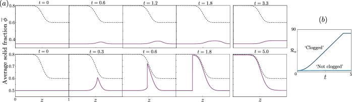
We obtain temporal solutions in regions of parameter space both with and without a steady numerical solution. For the former, the system reaches the steady state described above in which the solid fraction increases slightly within the constricted part of the channel (figure 4a). By contrast, in the “no solution” region of parameter space, the solid fraction increases significantly downstream, eventually forming a shock just upstream of the constriction. The shock then travels upstream all the way back to the inlet (figure 4a). As the shock passes through the inlet, the solid fraction increases to a much higher value, which we designate , and a new steady state is reached. This steady state corresponds to the point where a horizontal line extended from the red star marker in figure 3(c) meets the right hand side boundary of the no solution region. We find that this holds for any initial condition within the no solution region of the phase plot: the system will evolve to this “clogged-like” steady state with a much higher inlet particle fraction, and a much higher flow resistance. The clogged-like steady state can be constructed directly by setting the inlet solid flux in figure 3(a) equal to the maximum flux at the most constricted part of the channel. The steady-state solution with emergent heterogeneity corresponds to where the higher solution branch intersects with this new solid flux .
These features are reflected by determining the steady state at a fixed given by varying the inlet solid fraction (e.g. following the dashed horizontal line in figure 3c). The drastic increase in upon entering the “no solution” region, and the corresponding dramatic increase in the overall flow resistance, are illustrated in figure 4(d) and (e). These plots highlight the emergence of a “clogged” state from an initially unclogged state if the system is pushed above a critical volume fraction, given by the black region in the phase plot of figure 3(c).
As a proof of principle, we also performed temporal simulations in straight pipes but with a variation in the maximum particle fraction from high to low (figure 5), to represent variation in particle properties caused by biological processes such as cell stiffening in sickle cell disease. Again, we find a bifurcation in the steady solutions: if the incident particle fraction is too large relative to the downstream maximum particle fraction , then the incident solid flux cannot be maintained and a shock forms (figure 5 bottom row). Again the system evolves to a solution with a much higher inlet solid fraction, and a much larger overall flow resistance (figure 5b), demonstrating that our predictions of emergent heterogeneity in solid fraction apply to a broad range of particulate suspensions in which either geometry or particle properties vary in space.
4 Discussion
We have built a mechanistic model that allows for spatio-temporal variations in the volume fraction of particle suspensions flowing through a pipe. A key benefit of our approach, which splits suspension flow into a “wet solid” phase and a differential Darcy phase, is that the constitutive properties of each phase are clear and measurable. In our model, spatio-temporal volume fraction variations arise spontaneously when there are constrictions, and can result in an abrupt transition to a high-particle-fraction “clogged” state. This transition follows from the existence of a maximal solid flux at an intermediate particle fraction, which depends on geometry and particle properties and can therefore vary in space. The emergence of clogging occurs when the flux in one region of space is higher than the maximal flux in another region.
Our model complements existing stochastic and discrete theories for the effect of constrictions on particle suspensions – our macroscopic, deterministic approach captures these effects mechanistically over long length and time scales. For example, previous work on clogging [16, 22, 26] has identified a probability of bridging which is reflected at the macroscale in our model by an increased resistance of the suspension phase, which forces fluid to flow differentially through the Darcy phase.
The most relevant additional physics to be incorporated into our model for comparison with experiments is the inclusion of particle slip on the walls. Allowing for slip would allow for the prediction of a jammed but flowing state, as observed experimentally [23]. Improvements could also be made in capturing the rheology of deformable particles and relaxing the lubrication approximation to describe pipes with sharper along-flow variations in their properties.
We would like to acknowledge numerous helpful discussions with Valeria Ciccone, Anne Juel, Hannah Szfraniec, David Wood, Parisa Bazazi, John Higgins and Howard Stone. Declaration of interests. The authors report no conflict of interest. P.P. is supported by a UKRI Future Leaders Fellowship [MR/V022385/1].
References
- Ahnert et al. [2019] Ahnert, T., Münch, A. & Wagner, B. 2019 Models for the two-phase flow of concentrated suspensions. Eur. J. Appl. Math. 30, 557–584.
- Barker et al. [2015] Barker, T., Schaeffer, D. G., Bohorquez, P. & Gray, J. M. N. T. 2015 Well-posed and ill-posed behaviour of the -rheology for granular flow. Journal of Fluid Mechanics 779, 794–818.
- Baumgarten & Kamrin [2019] Baumgarten, A. S. & Kamrin, K. 2019 A general fluid-sediment mixture model and constitutive theory validated in many flow regimes. J. Fluid Mech. 861, 721–764.
- Boyer et al. [2011] Boyer, F., Guazzelli, É. & Pouliquen, O. 2011 Unifying suspension and granular rheology. Phys. Rev. Lett. 107.
- Bächer et al. [2017] Bächer, C., Schrack, L. & Gekle, S. 2017 Clustering of microscopic particles in constricted blood flow. Phys. Rev. Fluids 2.
- Clawpack Development Team [2024] Clawpack Development Team 2024 Clawpack software. Version 5.10.0.
- Cohen & Mahadevan [2013] Cohen, S. I. A. & Mahadevan, L. 2013 Hydrodynamics of hemostasis in sickle-cell disease. Phys. Rev. Lett. 110.
- Dincau et al. [2023] Dincau, B., Dressaire, E. & Sauret, A. 2023 Clogging: The self-sabotage of suspensions. Physics Today 76, 24–30.
- Dressaire & Sauret [2017] Dressaire, E. & Sauret, A. 2017 Clogging of microfluidic systems. Soft Matter 13, 37–48.
- Fahraeus & Lindqvist [1930] Fahraeus, R. & Lindqvist, T. 1930 The viscosity of the blood in narrow capillary tubes. J. Physiol. .
- Farutin et al. [2018] Farutin, A., Shen, Z., Prado, G., Audemar, V., Ez-Zahraouy, H., Benyoussef, A., Polack, B., Harting, J., Vlahovska, P. M., Podgorski, T., Coupier, G. & Misbah, C. 2018 Optimal cell transport in straight channels and networks. Phys. Rev. Fluids 3.
- Guazzelli & Pouliquen [2018] Guazzelli, E. & Pouliquen, O. 2018 Rheology of dense granular suspensions. J. Fluid Mech. 852.
- Holloway et al. [2011] Holloway, W., Aristoff, J. M & Stone, H. A 2011 Imbibition of concentrated suspensions in capillaries. Phys. Fluids 23 (8).
- Koh et al. [1994] Koh, C. J., Hookham, P. & Leal, L. G. 1994 An experimental investigation of concentrated suspension flows in a rectangular channel. J. Fluid Mech. 266, 1–32.
- Lyon & Leal [1998] Lyon, M. K. & Leal, L. G. 1998 An experimental study of the motion of concentrated suspensions in two-dimensional channel flow. Part 1. Monodisperse systems. J. Fluid Mech. 363, 25–56.
- Marin et al. [2018] Marin, A., Lhuissier, H., Rossi, M. & Kähler, C.J. 2018 Clogging in constricted suspension flows. Phys. Rev. E 97.
- Marin & Souzy [2024] Marin, A. & Souzy, M. 2024 Clogging of noncohesive suspension flows. Annu. Rev. Fluid Mech. 57, 89–116.
- Mondal et al. [2016] Mondal, S., Wu, C. H. & Sharma, M. M. 2016 Coupled CFD-DEM simulation of hydrodynamic bridging at constrictions. Int. J. Multiph. Flow 84, 245–263.
- Ness et al. [2022] Ness, C., Seto, R. & Mari, R. 2022 The physics of dense suspensions. Annu. Rev. Condens. Matter Phys. 13, 97–117.
- Parry & Millet [2010] Parry, A. J. & Millet, O. 2010 Modeling blockage of particles in conduit constrictions: Dense granular-suspension flow. J. Fluids Eng. 132, 0113021–01130210.
- Phillips et al. [1992] Phillips, R. J., Armstrong, R. C., Brown, R. A., Graham, A. L. & Abbott, J. R. 1992 A constitutive equation for concentrated suspensions that accounts for shear-induced particle migration. Phys. Fluids A 4, 30–40.
- Souzy et al. [2020] Souzy, M., Zuriguel, I. & Marin, A. 2020 Transition from clogging to continuous flow in constricted particle suspensions. Phys. Rev. E 101.
- Szafraniec et al. [2022] Szafraniec, H. M., Valdez, J. M., Iffrig, E., Lam, W. A., Higgins, J. M., Pearce, P. & Wood, D. K. 2022 Feature tracking microfluidic analysis reveals differential roles of viscosity and friction in sickle cell blood. Lab Chip 22, 1565–1575.
- Wood et al. [2012] Wood, D. K., Soriano, A., Mahadevan, L., Higgins, J. M. & Bhatia, S. N. 2012 A biophysical indicator of vaso-occlusive risk in sickle cell disease. Sci. Transl. Med. 4 (123), 123ra26–123ra26.
- Zimmermann et al. [2016] Zimmermann, U., Smallenburg, F. & Löwen, H. 2016 Flow of colloidal solids and fluids through constrictions: Dynamical density functional theory versus simulation. J. Phys. Condens. Matter 28.
- Zuriguel et al. [2014] Zuriguel, I., Parisi, D. R., Hidalgo, R. C., Lozano, C., Janda, A., Gago, P. A., Peralta, J. P., Ferrer, L. M., Pugnaloni, L. A., Clément, E., Maza, D., Pagonabarraga, I. & Garcimartín, A. 2014 Clogging transition of many-particle systems flowing through bottlenecks. Scientific Reports 4.