Hypergraph Link Prediction via Hyperedge Copying

Abstract.

We propose a generative model of temporally-evolving hypergraphs in which hyperedges form via noisy copying of previous hyperedges. Our proposed model reproduces several stylized facts from many empirical hypergraphs, is learnable from data, and defines a likelihood over a complete hypergraph rather than ego-based or other sub-hypergraphs. Analyzing our model, we derive descriptions of node degree, edge size, and edge intersection size distributions in terms of the model parameters. We also show several features of empirical hypergraphs which are and are not successfully captured by our model. We provide a scalable stochastic expectation maximization algorithm with which we can fit our model to hypergraph data sets with millions of nodes and edges. Finally, we assess our model on a hypergraph link prediction task, finding that an instantiation of our model with just 11 parameters can achieve competitive predictive performance with large neural networks.

Introduction

Many complex systems are composed of simple components participating in multi-way interactions. Such systems — often called higher-order networks [10] to distinguish them from networks composed of only pairwise interactions — have received much attention in recent years. Higher-order networks preserve richer structural information about a system and therefore admit a broader array of measures, dynamics, and algorithms than their pairwise counterparts [7, 6, 13]. Higher-order networks are frequently represented as either hypergraphs or simplicial complexes [3]. Whether a given system demands a higher-order representation, and which one to choose, are subtle modeling questions [42] driven by both the data analysis techniques to be used and the structure of the data itself.

Hypergraphs are among the most flexible data structures for representing higher-order networks. In hypergraphs, each multi-way interaction is represented by an edge consisting of a set of nodes of arbitrary finite size. While simplicial complex representations require that every subset of every edge is also present in the data, hypergraphs require no such stipulation. Empirically, many hypergraphs come close to satisfying this subset inclusion criterion, but many others do not [23]. While many hypergraph data sets include only the memberships of nodes in edges, other data sets may include node attributes [4], directedness or generalized node-edge roles [18, 15], and temporal information about the arrival or duration of interactions [27, 33]. The latter case is often described under the heading of temporal hypergraphs, and is our modeling focus in this paper. Some examples of systems naturally represented by temporal hypergraphs include group socializing, email communication, and scholarly collaboration [34, 38, 12].

A common aim in modeling temporal hypergraphs is link prediction, first popularized for dyadic graphs [28]: given observations of the hypergraph up to a specified time, we aim to predict which possible new edges are likely to form in the future. The link prediction problem in hypergraphs has a wide range of applications: in collaboration networks, predicting future collaborations among multiple entities can aid in resource allocation and project planning [47]; in biological systems, forecasting interactions among a set of molecules can contribute to drug discovery and understanding molecular processes [41]; in logistics and supply chain management, predicting future connections in a hypergraph can optimize the flow of goods and resources [40]. The problem of link prediction in hypergraphs was popularized by Benson et al. [8] and has since received treatment from a wide range of approaches [29, 46], with techniques including linear discriminative models [8], neural discriminative models [44], statistical generative models [37], and mechanistic generative models [9, 2, 20, 19].

We take a mechanistic approach to the modeling of temporal hypergraphs. Our modeling framework is motivated by a simple, fundamental difference between hypergraphs and dyadic graphs. In dyadic graphs, all edges contain two nodes (ignoring self-loops). Any pair of edges can therefore intersect on zero, one, or two nodes. The number of two-edge motifs [31] in undirected graphs (in which self-loops are disallowed but multiedges are allowed) is therefore three. In contrast, in hypergraphs, an edge of size $i$ may intersect with another edge of size $j$ on a set of any size $k\leq\min\{i,j\}$. The number of possible two-edge motifs in a hypergraph [26, 30] with maximum edge-size $\bar{k}$ is therefore $O(\bar{k}^{3})$, since the sizes of two edges, as well as the size of the intersection can all be distinguished. A wide range of intersection behavior is observed in empirical hypergraph data [25], at rates much higher than explained by simple null models [14].

Several generative models have been proposed which produce large hypergraph edge intersections [24]. The model of Lee, Choe, and Shin [25] reproduces several empirical intersection patterns in a hypergraph with specified edge-size and node degree distributions. Because these features of the data are specified in advance, the model is statistically generative but does not model mechanistic evolution in growing hypergraphs. The Correlated Repeated Unions (CRU) model of Benson, Kumar, and Tomkins [9] is an explicitly mechanistic and temporal hypergraph model: arriving edges are formed as unions of noisy copies of previous edges. Copy models have a rich history in network science, serving, for example, as an early alternative to preferential attachment as a mechanistic explanation for heavy tails in the degree sequences of dyadic graphs [21, 39, 43, 35]. The CRU model is designed to generate hypergraphs in which the same subsets of nodes appear in multiple edges. This model, however, is designed for subsampled hypergraphs which may be viewed as single “sequences of sets.” Applying the model to a full hypergraph dataset requires the researcher to subsample the data into one or more such sequences; this limits the model’s ability to describe hypergraphs in which seemingly disparate sequences may merge, and also prevents the researcher from evaluating a model likelihood on the complete data. Roh et al. [36] details the degree distribution and edge-size distribution for a model of growing hypergraphs with preferential linking in which the evolution of the hypergraph is based entirely on adding new nodes to current edges and nodes. Our proposed model is perhaps most similar to the hypergraph preferential attachment models proposed by Avin et al. [2] and Giroire et al. [20] involve several types of updates to the hypergraph, such as isolated vertex addition and multiple types of edge addition. In each timestep, one of these actions is selected and performed. In contrast, our model involves a single, multipart update step.

Our proposed Hyperedge Copy Model (HCM) employs a simple edge-copying growth mechanism. In each timestep, a new edge is formed as a noisy copy of an existing edge that was formed at a prior time, supplemented with nodes existing elsewhere in the hypergraph and novel nodes added after copying. In Methods, we describe the model update and derive asymptotic descriptions of the edge-size distribution, node degree distribution, and edge intersection rates. The generative nature of this HCM also provides a principled statistical framework for fitting and evaluating model fit to data. However, because we do not observe the identity of the edge which is (noisily) copied in each timestep, direct optimization of the model likelihood is intractable. Instead, we develop a stochastic expectation-maximization algorithm [11] for the inference task. In Results, we use stochastic expectation-maximization to fit our model to 27 empirical hypergraphs of sizes spanning several orders of magnitude. We also evaluate the fitted model on a hyperedge prediction task, finding competitive predictive performance benchmarking against neural network methods despite the extremely low-dimensional parameter space of the model. We close with discussion and suggestions for model generalizations.

Methods

Hyperedge Copy Model (HCM)

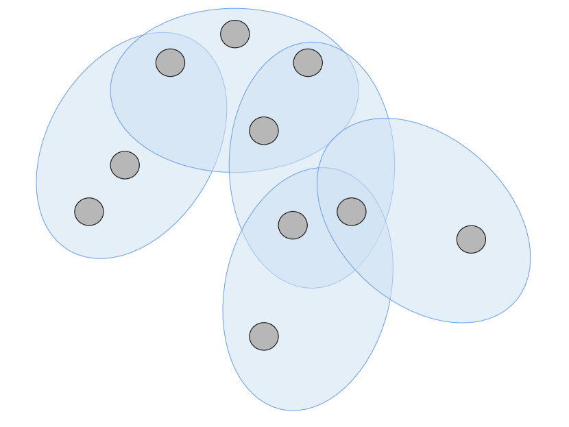
(a) Current hypergraph $\mathcal{H}^{(t)}$.

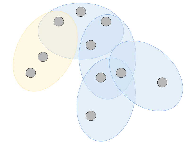
(b) Edge selection: An edge $f$ is selected uniformly at random (u.a.r.) from $\mathcal{E}^{(t)}$ and a node $v_{0}$ is selected u.a.r. from $f$ to seed the new edge $e^{(t+1)}$.

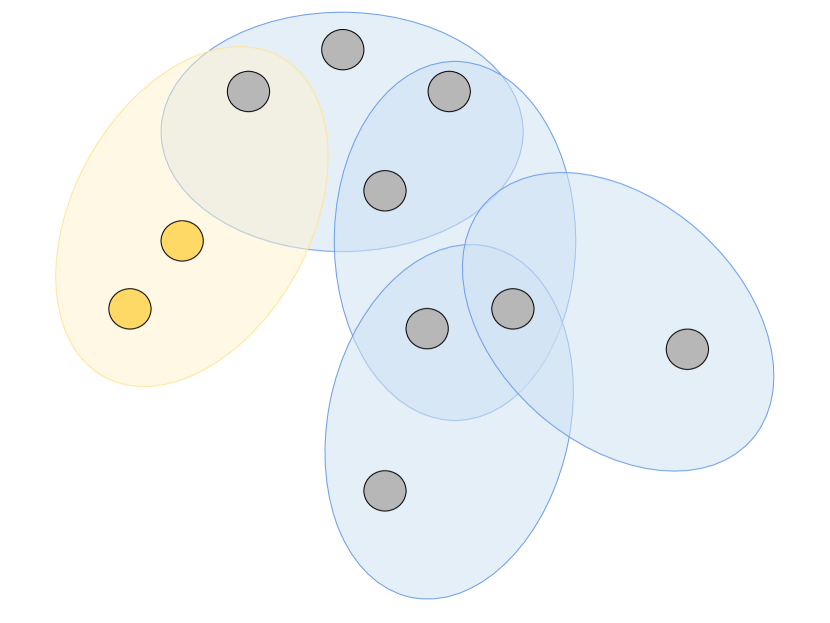
(c) Edge sampling: The remaining nodes $v\in f\setminus\left\{v_{0}\right\}$ are each selected i.i.d. with probability $\eta$ for inclusion in $e^{(t+1)}$.

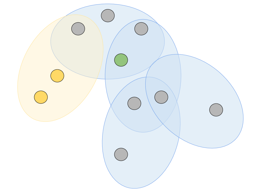
(d) Extant node addition: A number $g\sim\boldsymbol{\gamma}$ is sampled. Then, a set of $g$ distinct nodes is sampled u.a.r. from $\mathcal{N}^{(t)}\setminus f$ and added to $e^{(t+1)}$.

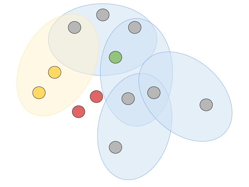
(e) Novel node addition: A number $b\sim\boldsymbol{\beta}$ is sampled. Then, a set of $b$ distinct nodes is created and added to both $\mathcal{N}^{(t+1)}$ and $e^{(t+1)}$.

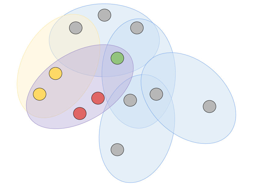
(f) Edge $e^{(t+1)}$ is added to $\mathcal{E}^{(t+1)}$.

Figure 1. Schematic illustration of the edge generation process for our Hyperedge Copy Model (HCM).

Our proposed model generates a sequence of growing hypergraphs. At each discrete timestep $t$, let $\mathcal{H}^{(t)}=(\mathcal{N}^{(t)},\mathcal{E}^{(t)})$ be a hypergraph with node set $\mathcal{N}^{(t)}$ and edge set $\mathcal{E}^{(t)}$. Each hyperedge $e\in\mathcal{E}^{(t)}$ is a named set of nodes $e\subseteq\mathcal{N}^{(t)}$. Multiedges — in which two distinctly named edges are equal as sets — are permitted. The degree of node $v$ in hypergraph $\mathcal{H}^{(t)}$ is $d^{(t)}_{v}=\sum_{e\in\mathcal{E}^{(t)}}\text{1}\!\!\left[v\in e\right]$, the number of edges containing $v$ in $\mathcal{E}^{(t)}$.

We consider only a single method of updating the hypergraph from time $t$ to time $t+1$, which consists of the following four substeps:

1. Edge selection: a single edge $f$ is selected uniformly at random (u.a.r.) from $\mathcal{E}^{(t)}$. Then, one node $v_{0}$ is selected u.a.r. from $f$ to seed the new edge $e^{(t+1)}$.

2. Edge sampling: the remaining nodes $v\in f\setminus\left\{v_{0}\right\}$ are each included in $e^{(t+1)}$ independently with probability $\eta\in[0,1]$.

3. Extant node addition: a nonnegative integer $g$ is sampled from a distribution which we express as a probability vector $\boldsymbol{\gamma}$. We require that $\boldsymbol{\gamma}$ be an element of $S^{\bar{k}}$, where $S^{\bar{k}}$ is the set of probability vectors indexed $0$ through $\bar{k}$. The choice of $\bar{k}$ gives the largest possible number of extant nodes which can be added in a single update step. With a slight abuse of notation, we write $g\sim\boldsymbol{\gamma}$ to denote this sampling process. Then, $g$ distinct nodes are selected u.a.r. from $\mathcal{N}^{(t)}$ and added to $e^{(t+1)}$.

4. Novel node addition: a nonnegative integer $b\sim\boldsymbol{\beta}$ is sampled, where again $\boldsymbol{\beta}$ is a probability vector, and $b$ distinct nodes are created and added to $e^{(t+1)}$.

After forming $e^{(t+1)}$, we define the updated hypergraph $\mathcal{H}^{(t+1)}=(\mathcal{N}^{(t)}\cup\left\{e^{(t+1)}\right\},\mathcal{E}^{(t)}\cup{e^{(t+1)}})$. Algorithm 1 gives a formalized summary of the model, and Figure 1 gives a schematic graphical illustration. The parameters of the model are the copy probability $\eta$, the extant node distribution $\boldsymbol{\gamma}$, and the novel node distribution $\boldsymbol{\beta}$. For notational compactness, we will use the vector $\boldsymbol{\theta}=(\eta,\boldsymbol{\gamma},\boldsymbol{\beta})$ to refer to the concatenation of these three parameters. The total number of scalar parameters of the model is $2\bar{k}+1$.

Algorithm 1 Hyperedge Copy Model (HCM) update step

$\mathcal{H}^{(t)}=\left(\mathcal{N}^{(t)},\mathcal{E}^{(t)}\right)$, $\eta\in[0,1]$, $\boldsymbol{\gamma}\in S^{\bar{k}}$, $\boldsymbol{\beta}\in S^{\bar{k}}$

$e\leftarrow\emptyset$

Sample $f\sim\mathrm{Uniform}\left(\mathcal{E}^{(t)}\right)$ $\triangleright$ Edge selection

Sample $v_{0}\sim\mathrm{Uniform}\left(f\right)$ $\triangleright$ Edge sampling

$e^{(t+1)}\leftarrow e\cup\left\{v_{0}\right\}$

for node $v\in f\setminus v_{0}$ do

  With probability $\eta$, $e^{(t+1)}\leftarrow e^{(t+1)}\cup\left\{v\right\}$

Sample $g\sim\boldsymbol{\gamma}$ $\triangleright$ Extant node addition

Sample $V\sim\mathrm{Uniform}\left(\genfrac{}{}{0.0pt}{2}{\mathcal{N}^{(t)}\setminus f}{g}\right)$

$e^{(t+1)}\leftarrow e^{(t+1)}\cup V$

Sample $b\sim\boldsymbol{\beta}$ $\triangleright$ Novel node addition

$n\leftarrow\left\lvert\mathcal{N}^{(t)}\right\rvert$

$\mathcal{N}^{(t+1)}\leftarrow\mathcal{N}^{(t)}\cup\left\{v_{n+1},\ldots,v_{n+b}\right\}$

$e^{(t+1)}\leftarrow e^{(t+1)}\cup\left\{v_{n+1},\ldots,v_{n+b}\right\}$

$\mathcal{E}^{(t+1)}\leftarrow\mathcal{E}^{(t)}\cup e^{(t+1)}$

return $\mathcal{H}^{(t+1)}=\left(\mathcal{N}^{(t+1)},\mathcal{E}^{(t+1)}\right)$

Asymptotic degree and edge-size distributions

We now derive several asymptotic properties of our proposed HCM. We first derive the asymptotic mean edge size, as well as a linear system describing the complete edge size distribution. Let $\langle k\rangle$ be the mean edge size in $\mathcal{H}^{(t)}$. We will compute this mean under an assumption of stationarity. Each time an edge is constructed, there are in expectation $1+\eta(\langle k\rangle-1)$ nodes sampled in the edge sampling step, $\mu_{\boldsymbol{\gamma}}$ nodes sampled in the extant node addition step, and $\mu_{\boldsymbol{\beta}}$ nodes sampled in the novel node addition step, where $\mu_{\cdot}$ denotes the mean of the corresponding distribution. At stationarity, we therefore have the self-consistent equation

(1) $$\langle k\rangle=1+\eta(\langle k\rangle-1)+\mu_{\boldsymbol{\gamma}}+\mu_{\boldsymbol{\beta}}\;,$$

from which it follows that, provided $\eta<1$,

(2) $$\langle k\rangle=\frac{1-\eta+\mu_{\boldsymbol{\gamma}}+\mu_{\boldsymbol{\beta}}}{1-\eta}\;.$$

When $\eta=1$, the edge size is nonstationary and grows arbitrarily large, as reflected in the divergence of eq. 2.

To describe the edge size distribution, let $\mathbf{W}\in\mathbb{R}^{\bar{k}\times\bar{k}}$ be the matrix whose entry $w_{ij}$ gives the probability that the produced edge $e^{(t+1)}$ has size $i$ given that the sampled edge $f$ has size $j$. As we show in Section C.2, the entries of $\mathbf{W}$ have closed-form expressions in terms of the parameter vector $\boldsymbol{\theta}$:

(3) $$w_{ij}=\sum_{\ell=0}^{j-1}\sum_{h=0}^{i-\ell}\binom{j-1}{\ell}\eta^{\ell}(1-\eta)^{j-\ell-1}\gamma_{h}\beta_{i-\ell-h}\;.$$

The stationary distribution of edge sizes under our model is then given by the Perron eigenvector of the matrix $\mathbf{W}$. We give several examples of computing the stationary distribution of edge sizes for synthetic and empirical data sets using eq. 3 in Figure 5.

Turning now to the degree distribution, we first calculate the mean degree $\langle d\rangle$. In any hypergraph of $n$ nodes and $m$ edges, it holds that ${n}\langle d\rangle={m\langle k\rangle}$. At large $t$, in expectation $m/n\approx{1}/{\mu_{\boldsymbol{\beta}}}$, since on average there are $\mu_{\boldsymbol{\beta}}$ nodes added per new edge. Provided that $\eta<1$ (so that $\langle k\rangle$ is finite), we therefore have

(4) $$\langle d\rangle=\frac{\langle k\rangle}{\mu_{\boldsymbol{\beta}}}=\frac{1-\eta+\mu_{\boldsymbol{\gamma}}+\mu_{\boldsymbol{\beta}}}{\mu_{\boldsymbol{\beta}}(1-\eta)}\;.$$

Furthermore, the tails of the degree distribution are power-law with an exponent that depends on the model parameters. In Section C.1 we follow a derivation by Mitzenmacher [32] to argue that, for large $d$, the proportion $p_{d}$ of nodes with degree $d$ is approximated, for large $d$, by the power law $p_{d}\propto d^{-\zeta}$, where the exponent $\zeta$ is given by

(5) $$\zeta=1+\frac{1-\eta+\mu_{\boldsymbol{\gamma}}+\mu_{\boldsymbol{\beta}}}{1-\eta(1-\mu_{\boldsymbol{\gamma}}-\mu_{\boldsymbol{\beta}})}\;.$$

An intuitive explanation for the occurrence of a power law in this context is that the edge selection and sampling steps of the HCM choose nodes in proportion to the number of edges in which those nodes are present; i.e. their degree. Degree-proportional sampling is a classical mechanism for generating power-law degree distributions [5, 21]. We show examples of the power law exponent predicted by our model in comparison to synthetic and empirical data sets in Figure 5.

Asymptotic edge intersection sizes

It is possible to compute the exact asymptotic structure of the densities of pairwise intersections in our proposed model. We express this structure in terms of the joint distribution

(6) $$r_{ijk}\triangleq\rho\left(\left\lvert e\right\rvert=i,\left\lvert f\right\rvert=j,\left\lvert e\cap f\right\rvert=k\;\middle|\;|e\succ f\right)\;,$$

where $e\succ f$ indicates that edge $e$ appears later than edge $f$. We present a probabilistic argument in Section C.3 for a claim describing the asymptotic structure of the intersection sizes in our model. Under this claim, if $\beta_{0}<1$, there exist constants $q_{ijk}$ such that, as the number of edges $m$ grows large:

• The intersection sizes $r_{ijk}$ are related to the constants $q_{ijk}$ as

  (7) $$r_{ijk}=\begin{cases}q_{ijk}+O\left(m^{-1}\right)&\quad k=0\\ m^{-1}q_{ijk}+O\left(m^{-2}\right)&\quad\text{otherwise\;.}\end{cases}$$

• The constants $q_{ijk}$ can be computed as the entries of the unique nonnegative eigenvector of a matrix $\mathbf{C}$ determined by the parameters $\eta$, $\boldsymbol{\gamma}$, and $\boldsymbol{\beta}$.

These asymptotics are illustrated in Figure 2 on a large synthetic hypergraph simulated according to the HCM. We show the proportion $r_{k}=\sum_{ij}r_{ijk}$ of pairs of edges of any size intersecting on a set of size $k$ over time (left) and at the final timestep (right), and compare these to the asymptotic predictions of eq. 7. The predictions agree closely with simulated values, matching both the $m^{-1}$ scaling and the predicted intercepts.

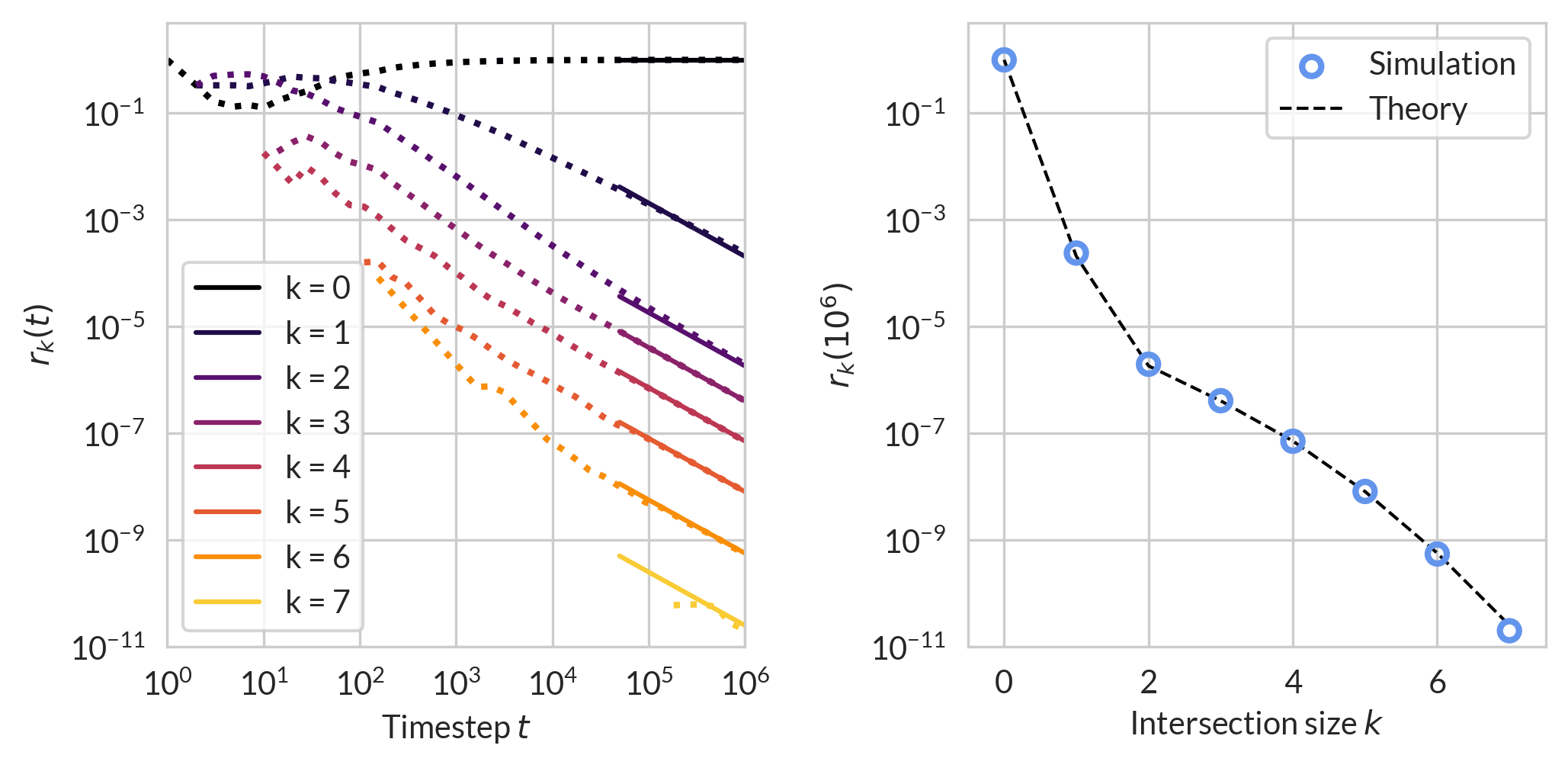
Figure 2. Illustration of the edge intersection asymptotics given by eq. 7. We simulated an HCM for $10^{6}$ timesteps with parameters $\eta=0.3$, $\boldsymbol{\beta}$ uniform on $\left\{1,2\right\}$, and $\boldsymbol{\gamma}$ uniform on $\left\{0,1\right\}$. (Left): Scaling of intersection size densities $r_{k}$ as a function of timestep $t$. Dotted lines give empirical intersection rates. Solid lines for $k\geq 1$ give the predicted scaling $m^{-1}\sum_{ij}q_{ijk}$, with $q_{ijk}$ computed as the entries of the leading eigenvector for a matrix $\mathbf{C}$ determined by the model parameters. Note the log-log axes. (Right): Proportion $r_{k}$ of pairs of edges intersecting on a set of size $k$ at the end of our simulation after $10^{6}$ timesteps, compared with predictions obtained from eq. 7.

Other asymptotic properties

Our HCM displays several other asymptotic structural properties which differ simpler models of evolving hypergraphs (Figure 3). We fit the HCM to the email-enron dataset using the stochastic expectation-maximization (SEM) algorithm described in the following section. We simulated a synthetic hypergraph generated according to the model. We also simulated two other synthetic hypergraphs: one generated according to a temporal Erdős-Rényi-type model (ER) that replicates the edge-size distribution of the fitted HCM, as well as a preferential attachment-type model (PA) which also replicates the power law degree distribution. Details on these two alternative models can be found in appendix D. We measured four structural properties of the empirical email-enron hypergraph and the three synthetic hypergraphs: uniform degree assortativity [14], clustering coefficient [17], edit simpliciality [23], and edge intersections [23] (values shown in Figure 3).

In the case of email-enron, we observe that the behavior of the HCM is quite distinct from that of the ER and PA models. The HCM replicates the degree assortativity less well than either the ER or PA models and replicates the clustering coefficient roughly as well as the ER model. For edit simpliciality and intersection sizes, the HCM does not quantitatively capture the correct measurement, but does qualitatively express that these quantities are not asymptotically vanishing, in contrast to the predictions by both the ER and PA models. We show the same experiment on several other datasets in Figure 9.

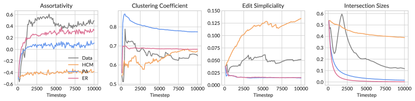
Figure 3. Structural properties of the email-enron temporal hypergraph and three synthetic models. We note that assortativity is highly dataset-dependent, and the behavior of different models changes drastically with different datasets. Specifically, for edge intersection size, we observe that only HCM has demonstrated non-diminishing intersection sizes over time steps, as shown in the same experiment on several other example datasets in Figure 9.

Inference via Stochastic Expectation Maximization (SEM)

We use maximum-likelihood estimation to learn the parameters $\eta$, $\boldsymbol{\gamma}$, and $\boldsymbol{\beta}$ of our proposed HCM from a dataset containing time-stamped hyperedges. The HCM has the structure of a latent-variable model: the edge $e^{(t+1)}$ that was added in timestep $t+1$ is observed, but the edge $f$ that was sampled in the edge-selection step to generate $e^{(t+1)}$ is not. This structure lends itself naturally to optimization via the expectation-maximization (EM) algorithm [16]. Let $F^{(t+1)}$ be the true but unobserved edge that was sampled in the edge-selection step. Given the observation of $e^{(t+1)}$ and some current estimate $\boldsymbol{\theta}$ of the parameters, the probability that the true $F^{(t+1)}$ was edge $f$ is

$$\mathbb{P}\left(F^{(t+1)}=f\;\middle|\;e^{(t+1)};\boldsymbol{\theta}\right) =\frac{\mathbb{P}\left(e^{(t+1)},F^{(t+1)}=f;\boldsymbol{\theta}\right)}{\mathbb{P}\left(e^{(t+1)};\boldsymbol{\theta}\right)}$$

$$=\frac{\mathbb{P}\left(e^{(t+1)},F^{(t+1)}=f;\boldsymbol{\theta}\right)}{\sum_{f^{\prime}}\mathbb{P}\left(e^{(t+1)},F^{(t+1)}=f^{\prime};\boldsymbol{\theta}\right)}\;$$

$$=\frac{\mathbb{P}\left(e^{(t+1)}\;\middle|\;F^{(t+1)}=f;\boldsymbol{\theta}\right)}{\sum_{f^{\prime}}\mathbb{P}\left(e^{(t+1)}\;\middle|\;F^{(t+1)}=f^{\prime};\boldsymbol{\theta}\right)}\;,$$

where the final line follows because the selection of $F^{(t+1)}=f$ in the HCM is uniform over the edge set $\mathcal{E}^{(t)}$. The probabilities appearing in this final expression are determined by Algorithm 1 and can be computed in closed form. The general EM algorithm applied to the single observation of $e^{(t+1)}$ proceeds by maximizing the expectation of the log-likelihood with respect to a new parameter estimate, with the expectation taken with respect to $\mathbb{P}\left(F^{(t+1)}=f\;\middle|\;e^{(t+1)};\boldsymbol{\theta}\right)$, which we now abbreviate $p^{(t+1)}(f;\boldsymbol{\theta})$ for notational compactness. In our case, this maximization problem has a closed-form solution in terms of the vector $\mathbf{s}$ of expected sufficient statistics of the distributions involved in sampling. This vector has components

(8) $$s_{1} =\sum_{f}p^{(t+1)}(f;\boldsymbol{\theta})\left\lvert f\cap e^{(t+1)}\right\rvert\;,$$

(9) $$s_{2} =\sum_{f}p^{(t+1)}(f;\boldsymbol{\theta})\left\lvert f\setminus e^{(t+1)}\right\rvert\;,$$

(10) $$s_{3,\ell} =\sum_{f}p^{(t+1)}(f;\boldsymbol{\theta})\text{1}\!\!\left[\left\lvert e^{(t+1)}\setminus\mathcal{N}^{(t)}\right\rvert=\ell\right]\;.$$

(11) $$s_{4,\ell} =\sum_{f}p^{(t+1)}(f;\boldsymbol{\theta})\text{1}\!\!\left[\left\lvert\left(e^{(t+1)}\setminus f\right)\cap\mathcal{N}^{(t)}\right\rvert=\ell\right]\;.$$

Once $\mathbf{s}$ is computed, the maximum likelihood estimates for the parameters are

(12) $$\hat{\eta}=\frac{s_{1}-1}{s_{1}+s_{2}-1}\;,\quad\hat{\gamma}_{\ell}=s_{3,\ell}\;,\quad\hat{\beta}_{\ell}=s_{4,\ell}\;.$$

Importantly, we are guaranteed that $s_{1}\geq 1$ by the requirement of Algorithm 1 that $\left\lvert f\cap e^{(t+1)}\right\rvert\geq 1$ for all $f$ with $p^{(t+1)}(f;\boldsymbol{\theta})>0$.

In standard, full-batch EM, we would compute averages of the expected sufficient statistics across the entire sequence of new edges, and then use eq. 12 to form new parameter updates. We would then repeat this process until convergence to a local maximum of the likelihood function, which is guaranteed by standard theory. For our setting, however, the full-batch EM algorithm is infeasible due to the computational cost of forming the distributions $p^{(t+1)}(f;\boldsymbol{\theta})$, requiring summation over all $t$ edges that arrived prior to time $t+1$. This sum thus includes order $m^{2}$ terms for each timestep, where $m$ is the number of edges in the hypergraph, which is computationally prohibitive for hypergraphs with $m\gtrsim 10^{4}$ on modern personal computers.

We therefore instead consider a stochastic variant of EM [11]. Starting from an arbitrary initial vector $\hat{\mathbf{s}}(0)$ of estimates of the expected sufficient statistics, we update with an exponentially moving average. In each algorithmic step $\tau$ of stochastic EM, we sample an edge $e$ uniformly at random. We then construct the vector $\mathbf{s}({\tau})$ of expected sufficient statistics from the observation of according to eqs. 8, 9, 10 and 11. Next, we update $\hat{\mathbf{s}}(\tau)$ according to

(13) $$\hat{\mathbf{s}}(\tau+1)=\left(1-\rho(\tau)\right)\hat{\mathbf{s}}(\tau)+\rho(\tau)\mathbf{s}(\tau).$$

Here, $\rho(\tau)$ is a learning schedule that determines the rate of update in the estimate of the expected sufficient statistics. The running estimate $\hat{\boldsymbol{\theta}}(\tau)$ of the parameter vector $\boldsymbol{\theta}$ is obtained from eq. 12, using $\mathbf{\hat{s}}(\tau)$ in place of $\mathbf{s}$. We use a learning schedule $\rho(\tau)=\tau^{-1}$ and terminate the algorithm when the relative change in the estimate of $\eta$ between the most recent 100-step windows falls below $10^{-2}$.

Results

SEM-HCM on empirical data

We used SEM to fit our HCM to 27 empirical hypergraphs provided by the XGI package for Python [22]. Clock-times to convergence ranged from 1.6 seconds in the case of the diseasome dataset (516 nodes and 903 edges) to $2.9\times 10^{4}$ seconds (8 hours) for the threads-stack-overflow dataset ($2.7\times 10^{6}$ nodes and $1.1\times 10^{7}$ edges). We give convergence times and more detailed descriptions of learned parameters in Table 3.

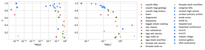
Figure 4. (Best viewed in color). Visual summary of parameters obtained by SEM fits of our HCM to empirical hypergraphs. We show $\eta$ and the expectations $\mu_{\boldsymbol{\beta}}=\sum_{i}i\beta_{i}$ and $\mu_{\boldsymbol{\gamma}}=\sum_{i}i\gamma_{i}$. We use linear scale for $\eta$ and log scale for $\mu_{\boldsymbol{\beta}}$ and $\mu_{\boldsymbol{\gamma}}$. When fitting the model using SEM, The default length $\bar{k}$ of $\boldsymbol{\beta}$ and $\boldsymbol{\gamma}$ is set to be equal to the largest edge size in the corresponding empirical hypergraphs. Coauthorship datasets are shown in orange; biological datasets in pink; information datasets in green, and social interaction datasets in blue.

Figure 4 summarizes the parameters obtained by SEM fits of our HCM to empirical hypergraphs. We group the datasets into four broad categories: coauthorship, biological, information, and social interaction. The social interaction networks in our dataset have very high rates $\eta$ of edge-copying, along with relatively low rates of extant or novel node addition. Coauthorship networks tend to display lower rates of edge-copying and higher rates of extant and novel node addition. Biological and information networks display less clear patterns, with different networks in these categories displaying very different estimated parameter values. On the whole, most datasets exhibit seemingly small values of $\mu_{\boldsymbol{\gamma}}$, consistently below one, indicating low rates of adding extant nodes elsewhere in the hypergraph to the edge being copied. The kaggle graph, however, stands out as an outlier among the larger hypergraphs, introducing a substantial number of new nodes at each timestep.

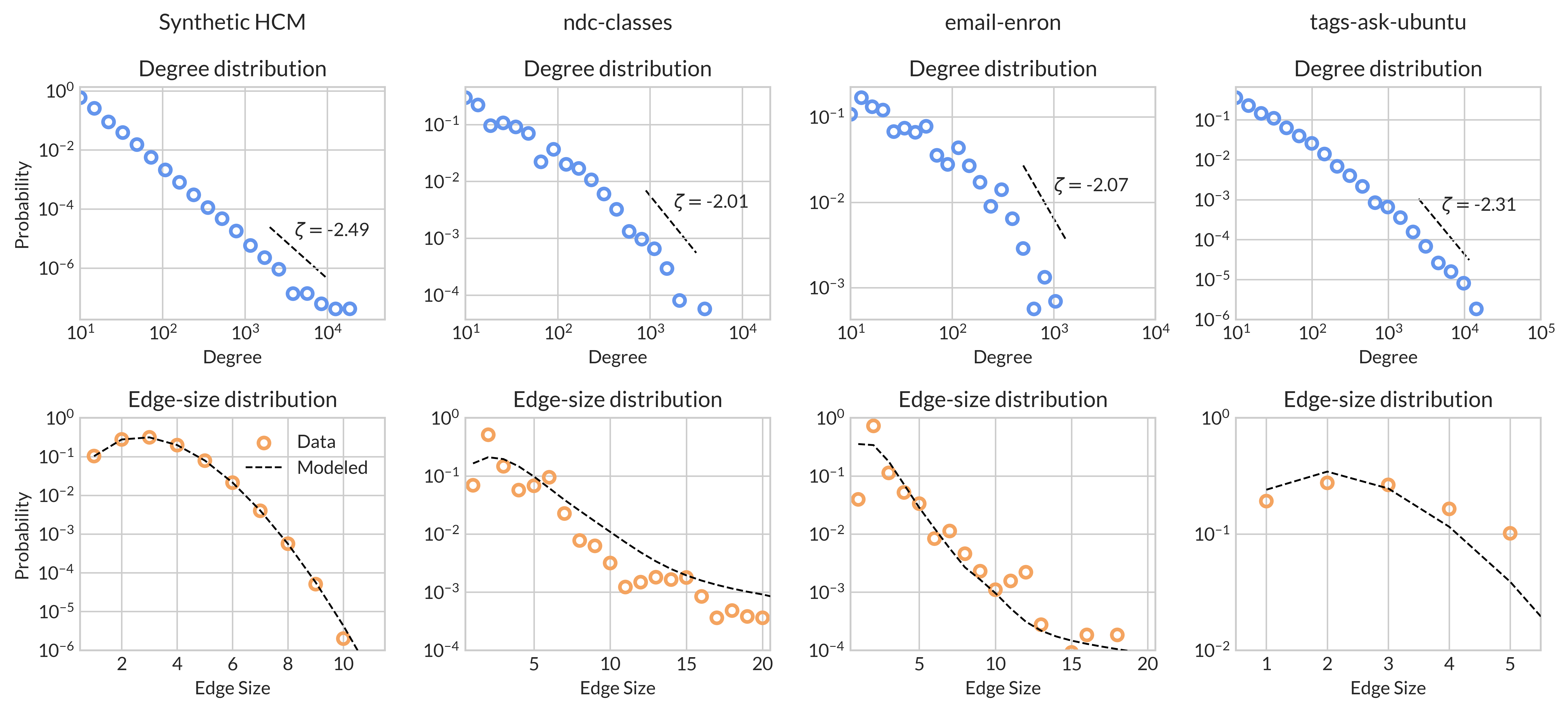
Figure 5. Degree distributions and edge-size distributions for one synthetic HCM with $10^{6}$ edges and three empirical datasets: ndc-classes, email-enron, and tags-ask-ubuntu. In the top row, dashed lines indicate the exponent of the power-law describing the asymptotic degree distribution using parameters inferred via SEM and eq. 20. In the bottom row, the dashed curve gives the modeled asymptotic edge-size distribution using inferred parameters to compute the matrix $\mathbf{W}$ described by eq. 3 and its associated Perron eigenvector. For the synthetic hypergraph (first column), the true parameters are used to construct the approximations and no inference is performed. The ndc-classes and email-enron edge-size distributions have been truncated for visualization purposes.

As one form of validation, we compare the actual degree and edge-size distributions of several datasets to the asymptotic descriptions provided by eqs. 3 and 20, using the parameters obtained by SEM. We show this comparison in Figure 5. We show the slope corresponding to the power-law exponent for the degree-distribution of the HCM as well as the complete modeled distribution of edge sizes. We find rough qualitative agreement in both cases, despite the small number of parameters that the HCM uses to describe each dataset. This appears true despite the considerable variety of network structures shown. Different empirical hypergraphs may exhibit quite different edge-size distributions: some, like congress-bills, have a small number of nodes but very large edges (see Table 1 below for sizes of each dataset), while others, like tags-ask-ubuntu, have much larger numbers of nodes but much smaller edges. The parameters from the SEM-HCM fit approximate the degree and edge-size distributions for these very different empirical hypergraphs.

Link prediction on empirical networks

Dataset	Type	$n$	$m$	$\bar{k}$	AUC	Recall	AUC(t)	Recall(t)
coauth-dblp	co-author	1,930,378	3,700,681	280	0.871	0.807	0.659	0.745
coauth-mag-geology	co-author	1,261,129	1,590,335	284	0.780	0.668	0.544	0.651
coauth-mag-history	co-author	1,034,876	1,812,511	925	0.639	0.607	0.367	0.464
dawn	biological	2,558	2,272,433	16	$-$	$-$	$-$	$-$
disgenenet	biological	12,368	2,261	2453	0.574	0.545	NA	NA
diseasome	biological	516	903	11	0.315	0.320	0.442	0.474
kaggle-whats-cooking	biological	6,714	39,774	65	0.945	0.903	NA	NA
ndc-classes	biological	1,161	49,726	39	0.989	0.973	0.988	0.973
ndc-substances	biological	5,556	112,405	187	0.558	0.544	0.616	0.615
tags-ask-ubuntu	webpage	3,029	271,233	5	0.763	0.738	0.697	0.650
tags-math-sx	webpage	1,629	822,059	5	0.740	0.665	0.624	0.589
tags-stack-overflow	webpage	49,998	14,458,875	5	$-$	$-$	$-$	$-$
threads-ask-ubuntu	webpage	125,602	192,947	14	0.507	0.608	0.429	0.601
threads-math-sx	webpage	176,445	719,792	21	0.754	0.778	0.674	0.731
threads-stack-overflow	webpage	2,675,969	11,305,356	67	0.778	0.779	0.686	0.774
congress-bills	social	1,718	282,049	400	0.575	0.540	0.528	0.465
contact-high-school	social	327	172,035	5	0.989	0.947	0.983	0.937
contact-primary-school	social	242	106,879	5	0.951	0.880	0.933	0.854
email-enron	social	148	10,885	37	0.944	0.882	0.755	0.707
email-eu	social	1,005	235,263	40	0.916	0.863	0.882	0.826
hospital-lyon	social	75	27,834	5	0.874	0.785	0.636	0.633
hypertext-conference	social	113	19,036	6	0.934	0.864	NA	NA
invs13	social	92	9,644	4	0.968	0.911	NA	NA
invs15	social	232	73,822	4	0.928	0.889	NA	NA
malawi-village	social	86	99,942	4	0.99	0.971	NA	NA
science-gallery	social	10,972	338,765	5	1.0	0.999	NA	NA
sfhh-conference	social	403	54,305	9	0.979	0.922	NA	NA

Table 1. Link prediction on the empirical hypergraphs provided by the XGI package for Python [22]. The number of nodes $n$, number of edges $m$, and maximum edge size $\bar{k}$ are shown for each dat set. We compute area under the receiver operating characteristic (AUC) and recall scores for models trained on timestamped sequences (t) and random sequences of edges, using $20\%$ of the total data in both cases. “NA” indicates that timestamps were not supplied for the dataset, making it impossible to perform link prediction under the (t) condition. AUC and recall scores are computed using either the remaining $80\%$ of data or $10^{5}$ edges sampled uniformly at random (in the case of large datasets) as positive examples, then generating an equal number of negative examples, and forming predictions on the examples as described in the main text. We did not obtain link prediction results for two of the datasets due to computational limitations in the evaluation of the marginal likelihood. We set the length of $\boldsymbol{\gamma}$ and $\boldsymbol{\beta}$ to be equal to the largest edge size for each empirical hypergraph for all runs.

At any given time, the HCM assigns a probability that any given candidate edge will indeed be formed in the next timestep. We can therefore perform link prediction using the HCM by predicting that high-probability candidates will be formed and that low-probability candidates will not.

A challenge in most link prediction contexts is the absence of true negative samples for training and evaluation. Because our model “training” is simply the SEM algorithm described above, we do not need negative samples for training; we do, however, still need them for evaluation. We therefore form a collection of negative examples by sampling non-realized edges in order to match the degree distribution and edge-size distribution of each empirical network. To do this, we draw the edge size for each created negative edge set of nodes according to the same empirical edge-size distribution of the (positive) edges while sampling nodes to be included in the negative set based on the node degree distribution. To maintain balanced classes, we generate as many negative examples as there are positive examples.

In each dataset, we use $20\%$ of the observed (positive) edges to perform SEM. We fit our model using two distinct types of training data. When timestamped data is available, we take the first $20\%$ of edges as training data. However, for each dataset, we also fit on a uniformly random subset of $20\%$ of the training data, which is not temporally contiguous. We use this strategy in order to assess the effectiveness of our model, which has explicit temporal structure, for settings in which no empirical timestamps are available. To assess the models trained under each condition, we combine the positive and negative examples and compute the probability of each candidate being realized under the HCM. We consider a positive prediction to be a candidate with modeled probability above the median. From the model’s predictions, we compute area under the receiver-operating characteristic curve (AUC) and recall scores. These scores are shown in Table 1, with the (t) columns indicating the use of temporal information for model fitting.

We use a maximum of $10^{5}$ edges as positive examples for evaluation; for temporally trained models we use edges immediately following the training set, while in non-temporally trained models we use up to $10^{5}$ edges sampled uniformly at random. There were two extremely dense datasets (dawn and tags-stack-overflow) in which we were able to perform inference via SEM but not able to perform link prediction due to the computational expense of computing the marginal log-likelihood of a candidate edge. In such hypergraphs, the number of candidate edges $f$ which could have generated a new edge $e$ is very large, leading to many terms in the marginal log-likelihood which must be computed.

Perhaps surprisingly considering that our HCM relies heavily on temporal information, the link prediction results from random draws of edges ignoring the temporal timestamp information are in many cases as good or better than the predictions obtained from using the temporal ordering supplied with the data. Indeed, our model was especially successful on many social interaction datasets for which no timestamps are supplied with the data (bottom rows of Table 1). Despite the small number of parameters in the HCM, we are able to achieve AUCs over $0.85$ in 14 out of 25 datasets for which we were able to perform link prediction.

We now compare the predictive performance of our HCM to that of two neural network methods: neural network methods, Neural Hypergraph Link Prediction (NHP) [44] and the Logical Hyperlink Predictor (LHP) [45]. The NHP study [44] shows results on 5 datasets and the LHP study [45] shows results on 4 datasets. We test our HCM on the three of these datasets that appear in both papers, replicating the experimental setup from these studies as closely as possible. We compute AUC and F1 scores for link prediction, as well as training time, and compare our results to the published results for NHP and LHP. To ensure comparability, we follow the same training setup: we use a uniformly random $20\%$ of hyperedges for training and use the rest for testing. We also follow the same approach for generating negative examples: for each positive hyperedge, we create a corresponding negative sample by randomly replacing half of the nodes in the edge set with edges from the rest of the hypergraph. Because these datasets are relatively small, we set both $\boldsymbol{\gamma}$ and $\boldsymbol{\beta}$ to a maximum length of $\bar{k}=5$ during training. Combined with $\eta$, this gives our model a total of 11 scalar parameters. The neural network models are much larger: while we do not have exact published parameter counts, information in the LHP paper gives at least $9.8\times 10^{5}$ scalar parameters.

We observe in Table 2 that our HCM performs competitively with the two neural network models: on the iJO1366 dataset it substantially outperforms both; on the iAF1260b dataset it performs better than NHP and worse than LHP; and on the USPTO dataset it performs worse than both NHP and LHP. We conjecture that the comparatively poor performance of our model reflects in part the small maximum edge size of this data set compared to the other two. Although our training times are typically larger than those reported for LHP, we note that LHP was trained on a TITAN RTX GPU while our model was trained on X. H.’s personal laptop, which possesses an 11th Gen Intel i7-11800H processor with 8 cores and 16 logical processors and 16GB of RAM.

	$n$	$m$	Max Edge Size	NHP AUC	NHP F1	NHP T	LHP AUC	LHP F1	LHP T	HCM AUC	HCM F1	HCM T
iAF1260b	1,668	2,084	67	0.582	0.415	1m22s	0.639	0.588	0m12s	0.605	0.539	0m42s
iJO1366	1,805	2,253	106	0.599	0.400	1m50s	0.638	0.620	0m17s	0.774	0.786	0m48s
USPTO	16,293	11,433	8	0.662	0.500	6m15s	0.733	0.650	1m35s	0.515	0.554	0m16s

Table 2. Link prediction results of our HCM against two neural network hypergraph link prediction methods, NHP [44] and LHP [45]. The iAF1260b and iJO1366 datasets are metabolic reaction hypergraphs while USPTO is an organic reactions hypergraphdataset. Negative edges are generated according to the description and code for LHP. Since none of these datasets are temporal hypergraphs, results are calculated from $20\%/80\%$ training-testing splits over 10 independent randomized trials. We set the lengths of both $\boldsymbol{\gamma}$ and $\boldsymbol{\beta}$ to be $5$ for all runs. The reported AUC and F1 scores for LHP and NHP are taken from Table 4 of the LHP paper [45]. The original NHP paper presents lower AUC scores compared to those reported in the LHP paper, possibly due to randomization; the higher of the two reported scores were used here. The times to train the models (“T”) are also taken from the LHP paper (Table 7), which used an NVIDIA TITAN RTX GPU. Time for fitting the HCM parameters was measured on X. H.’s personal computer, which possesses a a 11th Gen Intel i7-11800H that has 8 cores and 16 logical processors and 16GB of RAM.

Discussion

We proposed the Hyperedge Copy Model, a simple model of hypergraph evolution based on a noisy edge-copying mechanism. This model is mechanistic, interpretable, and analytically tractable. In addition to several analytic descriptions of the model’s behavior, we also provide a scalable stochastic expectation maximization algorithm for fitting the model to empirical data. We find in Table 2 that our 11-parameter model is competitive on link prediction tasks with neural network models containing hundreds of thousands of parameters.

One direction of future work concerns modeling of recombination of edges. In our HCM, new edges are formed from a noisy copy of a single prior edge. It may be of interest to allow edges to to form from multiple prior edges; such a process might model, for example, the formation of broad collaborations from multiple research groups. A version of this idea is explored in the context of sequences of sets by Benson et al. [9]. Incorporating such a mechanism into the HCM would significantly complicate the inference problem, since the set of possible generators of each edge would grow large. Fitting such a model to data might require more sophisticated computational techniques that could be of independent interest. Another direction of future work involves the incorporation of hypergraph metadata. In a hypergraph with node attributes, for example, one might model an edge sampling step in which the node $v_{0}$ sampled from the selected edge $e$ acts as a “leader” in the next edge; other edges in $e$ could be more likely to be copied into the next edge if they share attributes with $v_{0}$.

It is often claimed that the widespread availability of large data sets and computational power sufficient to train deep models has made theory and simple models obsolete in predictive tasks [1]. We take our results to suggest a continuing role for simple, interpretable stochastic models in the study of complex systems, even in the age of deep learning.

Software

We implemented our model and performed experiments using the XGI package [22] for higher-order network analysis in Python. The XGI package also makes available the datasets used in our experiments. (We conducted experiments using all datasets provided in the XGI package.) Code sufficient to fully reproduce our experiments is available at https://github.com/hexie1995/HyperGraph.

Acknowedgements

We thank Rebecca Hardenbrook, Nicholas Landry, Violet Ross, Alice Schwarze, and Anna Vasenina for helpful discussions. X.H. and P.J.M. were supported by the Army Research Office under MURI award W911NF-18-1-0244 and the National Institutes of Health FIC under R01-TW011493. P.S.C. was supported by the National Science Foundation Division of Mathematical Sciences under DMS-2407058. P.J.M. was additionally supported by the National Science Foundation under BCS-2140024 and DEB-2308460.

Appendix A Parameter estimation in synthetic HCM hypergraphs.

For consistency, we applied the same convergence criterion across all experiments in the paper. Specifically, every 100 steps, we calculated the difference between the current and previous $\eta$ values. If the percentage change was less than $1\%$, the loop was terminated. As examples, in Figure 6 we show the errors in the parameter estimates as obtained after different numbers of steps of the algorithm for two synthetic hypergraphs.

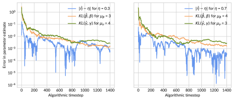
Figure 6. Estimation of parameters in two synthetic hypergraphs with 10k hyperedges each. The convergence criterion, tested every 100 steps, was reached at 1400 steps for each of them. We show the absolute difference $\left\lvert\hat{\eta}-\eta\right\rvert$ between the estimate and true value of $\eta$. We also show the Kullback–Leibler divergence of the estimates of $\boldsymbol{\beta}$ and $\boldsymbol{\gamma}$ from the true values. The $\beta$ and $\gamma$ here are generated with a random Poisson distribution, truncated at value $10$, with means $\mu_{\boldsymbol{\beta}}$ and $\mu_{\boldsymbol{\gamma}}$ indicated in the plot legends. Note the logarithmic scale of the vertical axis.

				Clock	Training
				time	steps
	$\eta$	$\mu_{\beta}$	$\mu_{\gamma}$	(s)	($\times 10^{3}$)
coauth-dblp	0.505	0.403	0.512	23.6	11
coauth-mag-	0.365	0.585	0.630	8.3	8
coauth-mag-history	0.242	0.202	0.110	14.0	18
dawn	0.686	4.15E-19	0.071	8064.3	4
disgenenet	0.099	6.90E-18	6.832	30.3	5
diseasome	0.078	6.23E-04	0.537	1.6	10
kaggle-whats-cooking	0.393	0.151	5.019	930.7	5
ndc-classes	0.996	0.009	0.019	41.1	3
ndc-substances	0.680	0.014	0.180	87.0	5
tags-ask-ubuntu	0.614	0.005	0.569	434.7	4
tags-math-sx	0.785	3.02E-04	0.197	1927.5	5
tags-stack-overflow	0.773	0.003	0.372	29212.2	4
threads-ask-ubuntu	0.058	0.477	0.468	46.6	13
threads-math-sx	0.165	0.191	0.848	85.8	4
threads-stack-overflow	0.082	0.149	1.007	92.6	6
congress-bills	0.294	0.003	1.379	563.2	5
contact-high-school	0.975	1.16E-04	0.034	81.0	3
contact-primary-school	0.910	8.25E-05	0.098	111.5	5
email-enron	0.887	0.013	0.083	24.8	3
email-eu	0.910	0.002	0.108	205.2	5
hospital-lyon	0.945	3.86E-05	0.069	148.9	4
hypertext-conference	0.888	2.63E-18	0.109	34.1	3
invs13	0.917	9.77E-08	0.082	23.8	4
invs15	0.938	4.11E-06	0.065	56.8	3
malawi-village	0.996	1.32E-18	0.005	168.8	3
science-gallery	0.871	2.10E-04	0.121	6.7	4
sfhh-conference	0.827	1.97E-20	0.185	69.3	5

Table 3. Details of parameters retrieved through stochastic expectation maximization with batch size 30 for each hypergraph. We set both the length of $\beta$ and $\gamma$ to be equivalent to the largest edge size in the corresponding real-world hypergraph.

Appendix B Reconstruction of Hypergraph Properties from Generative Models

In Figure 7, we compare the mean edge size and mean degree between hypergraphs generated from estimated parameters (listed in Table 3) and the original data, for a variety of real-world hypergraphs.

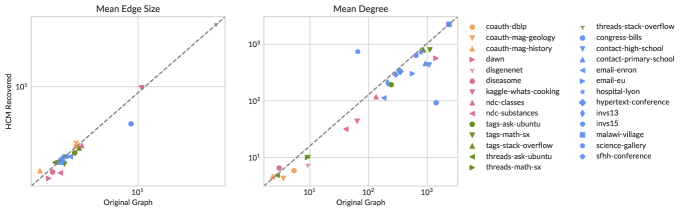
Figure 7. Mean edge sizes and mean node degrees compared between fit HCM instances and empirical data. Note the log-log scale.

We perform a similar analysis for synthetic datasets, comparing different hypergraph properties, including face edit simplicity, which is a more localized concept indicating the number of subfaces needed to be added to the hypergraph to render a specific face a simplex. We observe minimal differences in degree assortativity and edit simplicity between the HCM and ER hypergraphs in Figure 8. However, discrepancies arise in the clustering coefficient and face edit simplicity. Particularly, we see the face edit simpliciality for ER hypergraphs dropped persistently over time, which is very different behavior from the HCM (except in the case when $\eta=0.7$ and $\mu_{\boldsymbol{\beta}}=1.3$, and even in that case the HCM face edit simpliciality is orders of magnitude larger than for the corresponding ER hypergraphs). As was shown in [23], face edit simpliciality is usually higher than $10^{-2}$ for real-world hypergraphs, and thus the real-world replication of the ER model is much worse than that of our HCM, which keeps steadily above $10^{-2}$ for all cases studied.

For the clustering coefficient, interestingly, we see in Figure 8 that the values from the ER and HCM are almost the same when $\mu_{\boldsymbol{\beta}}$ is small. However, when $\mu_{\boldsymbol{\beta}}=1.3$, the clustering coefficient quickly drops for the ER hypergraphs, but stays steady for the HCM model, which has values close to the real world hypergraph clustering coefficients described in [17]. These properties of our HCM with various parameter sets demonstrate the ability of the model to generate realistic-seeming hypergraphs, despite its small number of parameters.

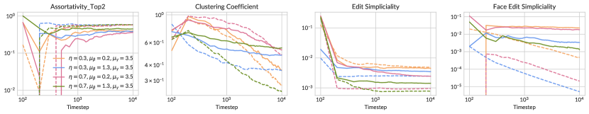
Figure 8. Hypergraph properties including top-2 degree assortativity, clustering coefficient, edit simpliciality, and face edit simpliciality from different generative models. Solid lines show values for data generated by the HCM. Dashed lines are for Erdős-Rényi hypergraphs generated with the same expected edge-size. The horizontal axis ranges from $t=0$ to $10$k, showing how the properties change with the numbers of steps in the growing hypergraphs.

In Figure 9, we repeat the experiment shown in Figure 3 for email-enron on other datasets, to demonstrate different exhibited behaviors across these other datasets, computing the assortativity, clustering coefficient, edit simpliciality, and intersection sizes for each dataset and the corresponding HCM, ER and PA models.

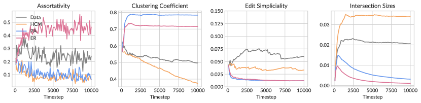
(a) email-eu

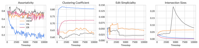
(b) ndc-classes

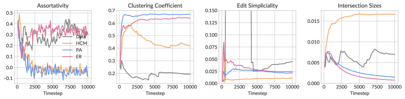
(c) ndc-substances

Figure 9. Structural properties of email-eu, ndc-classes, and ndc-substances. We show that these datasets have exhibited behaviors distinct from those of email-enron, shown in Figure 3 in the main text, highlighting that assortativity is highly dependent on the underlying structure of the real-world hypergraph. We also note that HCM is the only model that demonstrates non-diminishing edge intersection sizes across the different datasets.

Appendix C Asymptotic Properties

C.1. Power-law degree distribution

We now give a heuristic argument that the degree distribution of our model has an asymptotic power-law tail, with an exponent that depends on the model parameters. Our argument is based on rate equations, generalizing an argument by Mitzenmacher [32] in the context of preferential attachment dyadic graphs.

Fix $d>1$. Let $p^{(t)}_{d}$ be the proportion of nodes which have degree $d$ at time $t$. The total number of such nodes is $n^{(t)}p^{(t)}_{d}$. In timestep $t+1$, the change in the number of these nodes is $\Delta^{(t+1)}_{d}=n^{(t+1)}p^{(t+1)}_{d}-n^{(t)}p^{(t)}_{d}$. We now estimate $\delta^{(t+1)}_{d}=\mathbb{E}\left[\Delta^{(t+1)}_{d}\right]$ in expectation. The probability of an individual node being selected in the edge-sampling step is proportional to its degree $d$ in the current hypergraph $\mathcal{H}^{(t)}$, since there are $d$ edges which could be selected which contain that node. Normalizing, the probability that a given node selected in the edge-sampling step has degree $d$ is $\frac{d}{\langle d^{(t)}\rangle}p^{(t)}_{d}$, where $\langle d^{(t)}\rangle$ is the mean degree at time $t$. When a node of degree $d$ is selected in the edge-sampling step it becomes a node of degree $d+1$, while when a node of degree $d-1$ is selected it becomes a node of degree $d$. The expected number of nodes so selected is $1+\eta\left(\langle k^{(t)}\rangle-1\right)$, where $\langle k^{(t)}\rangle$ is the mean edge size at time $t$. Thus, the expected number of degree $d$ nodes created through the edge-sampling step is $\frac{1+\eta\left(\langle k^{(t)}\rangle-1\right)}{\langle d^{(t)}\rangle}\left[\left(d-1\right)p^{(t)}_{d-1}-dp^{(t)}_{d}\right]$. Through similar reasoning, the expected number of degree $d$ nodes created through the process of extant node addition is $\mu_{\boldsymbol{\gamma}}\left[p^{(t)}_{d-1}-p^{(t)}_{d}\right]$. Since we have assumed $d>1$ but novel node addition can only create nodes of degree $1$, only these two processes contribute. Our expected rate equation is then

(14) $$n^{(t+1)}p^{(t+1)}_{d}-n^{(t)}p^{(t)}_{d} =\frac{1+\eta\left(\langle k^{(t)}\rangle-1\right)}{\langle d^{(t)}\rangle}\left[\left(d-1\right)p^{(t)}_{d-1}-dp^{(t)}_{d}\right]+\mu_{\boldsymbol{\gamma}}\left[p^{(t)}_{d-1}-p^{(t)}_{d}\right]\;.$$

We now assume stationarity of the degree distribution and the edge size sequence. At stationarity, we must have $p^{(t+1)}_{d}=p^{(t)}_{d}=p_{d}$ for some constant $p_{d}$, as well as $\langle k^{(t)}\rangle=\langle k\rangle$ and $\langle d^{(t)}\rangle=\langle d\rangle$ for constants $\langle k\rangle$ and $\langle d\rangle$. We also have that $\langle d\rangle=\frac{m}{n}\langle k\rangle=\frac{\langle k\rangle}{\mu_{\boldsymbol{\beta}}}$, where we have used the fact that $\mu_{\boldsymbol{\beta}}$ nodes are added per edge in each timestep. Finally, in expectation, $n^{(t+1)}-n^{(t)}=\mu_{\boldsymbol{\beta}}$. At stationarity and in expectation, our approximate compartmental equation now reads

(15) $$\mu_{\boldsymbol{\beta}}p_{d}=a\left[\left(d-1\right)p_{d-1}-dp_{d}\right]+\mu_{\boldsymbol{\gamma}}\left[p_{d-1}-p_{d}\right]\;,$$

where we have defined $a=\frac{1+\eta\left(\langle k\rangle-1\right)}{\langle d\rangle}$. Rearrangement yields

(16) $$\frac{p_{d}}{p_{d-1}} =\frac{a(d-1)+\mu_{\boldsymbol{\gamma}}}{ad+\mu_{\boldsymbol{\gamma}}+\mu_{\boldsymbol{\beta}}}$$

(17) $$=1-\frac{a+\mu_{\boldsymbol{\beta}}}{ad+\mu_{\boldsymbol{\gamma}}+\mu_{\boldsymbol{\beta}}}\;.$$

Since we are interested in the tails of the degree distribution, we allow $d$ to grow large, yielding

(18) $$\frac{p_{d}}{p_{d-1}} \approx 1-\frac{a+\mu_{\boldsymbol{\beta}}}{a}\frac{1}{d}$$

(19) $$\approx\left(\frac{d-1}{d}\right)^{1+\frac{\mu_{\boldsymbol{\beta}}}{a}}\;.$$

Unfolding the recurrence yields, for large $d$, a power-law tail, $p_{d}\sim d^{-\zeta}$, with exponent $\zeta=1+\frac{\mu_{\boldsymbol{\beta}}}{a}$. Inserting explicit formulae for $a$, $\langle k\rangle$ (eq. 2) and $\langle d\rangle$ (eq. 4), we can express this exponent explicitly in terms of the model parameters using the formulas for $a$, $\langle k\rangle$, and $\langle d\rangle$, obtaining

(20) $$\zeta=1+\frac{1-\eta+\mu_{\boldsymbol{\gamma}}+\mu_{\boldsymbol{\beta}}}{1-\eta(1-\mu_{\boldsymbol{\gamma}}-\mu_{\boldsymbol{\beta}})}\;.$$

C.2. Edge-size distribution

We describe the entries of the matrix $\mathbf{W}$ described in the main text. Each entry $w_{ij}$ of $\mathbf{W}$ represents the conditional probability

(21) $$w_{ij}=\mathbb{P}\left(\left\lvert e\right\rvert=i\;\middle|\;\left\lvert f\right\rvert=j\right)\;,$$

where $f$ is the edge sampled in the edge-selection step of Algorithm 1 and $e$ is the final edge formed. We explicitly construct these probabilities conditional on the events that $\ell+1$ nodes are selected in the edge-sampling step and that $h$ nodes are selected in the extant node addition step. With these conditional probabilities, the law of total probability then yields

(22) $$w_{ij}=\mathbb{P}\left(\left\lvert e\right\rvert=i\;\middle|\;\left\lvert f\right\rvert=j\right)=\sum_{\ell=0}^{j-1}\sum_{h=0}^{i-\ell}\binom{j-1}{\ell}\eta^{\ell}(1-\eta)^{j-\ell-1}\gamma_{h}\beta_{i-\ell-h}\;.$$

The Perron eigenvector of this matrix gives the stationary distribution of edge sizes in the model. In practice, it is necessary to select a finite size for the matrix $\mathbf{W}$, which amounts to artificially setting $w_{ij}=0$ for $i$ and $j$ sufficiently large.

C.3. Asymptotic properties of intersection sizes

We now develop a probabilistic argument supporting the following claim:

Claim.

Let $r_{ijk}$ be the expected proportion of pairs of the $m$ edges, relative to the total number of pairs $\binom{m}{2}$, which have sizes $i$ and $j$ with intersection size $k$, with the expectation taken with respect to our proposed model and with the edge of size $j$ appearing before the edge of size $i$. Then, there exist constants $q_{ijk}\geq 0$ such that:

(23) $$r_{ijk}=\begin{cases}q_{ijk}+o(1)&\quad k=0\\ m^{-1}q_{ijk}+O(m^{-2})&\quad k\geq 1\;.\end{cases}$$

Furthermore, the scalars $q_{ijk}$ can be approximated as the solution of an eigenvector problem $\mathbf{q}=\mathbf{C}\mathbf{q}$, where $\mathbf{q}$ collects the scalars $q_{ijk}$ in flattened form and the matrix $\mathbf{C}$ is a function of the model parameters $\alpha$, $\boldsymbol{\beta}$, and $\boldsymbol{\gamma}$.

Throughout this section, we fix the timestep $t$. We use the shorthand $z\triangleq z^{(t)}$ and $z^{\prime}\triangleq z^{(t+1)}$ for any time-dependent quantities $z$. We also say that $f(m)\doteq g(m)$ if $\lim_{m\rightarrow\infty}\frac{f(m)}{g(m)}=1$, where $m$ is the number of edges in $\mathcal{H}$. We write $g\prec e$ if $e$ was added to $\mathcal{H}$ after $g$.

Let $R_{ijk}\triangleq\mathbb{P}^{(t)}\left(\left\lvert e\right\rvert=i,\left\lvert g\right\rvert=j,\left\lvert e\cap g\right\rvert=k\;\middle|\;g\prec e\right)$, where the probability is computed with respect to the empirical distribution of $\mathcal{E}^{(t)}$. The quantity $R_{ijk}$ corresponds to a sampling process in which we uniformly select a pair of edges; arrange them in descending order according to the timestep in which they were sampled; label the first (later) edge $e$ and the second (earlier) edge $g$; and then check whether $\left\lvert e\right\rvert=i$, $\left\lvert g\right\rvert=j$, and $\left\lvert e\cap g\right\rvert=k$. We will study the limiting behavior of $r_{ijk}\triangleq\mathbb{E}\left[R_{ijk}\right]$ as $t\rightarrow\infty$. Let $m=m^{(t)}$ and assume that one edge is added every timestep. Let $P_{ijk}\triangleq\binom{m}{2}R_{ijk}$ be the corresponding number of ordered pairs of edges of sizes $\left\lvert e\right\rvert=i$ and $\left\lvert g\right\rvert=j$ with intersection size $k$, ordered so that $g\prec e$. Let $p_{ijk}=\mathbb{E}\left[P_{ijk}\right]$.

We first write down a compartmental update for $P_{ijk}$ when a single edge $e$ is added. Assume that $e$ is sampled from edge $f$ in the edge-sampling step. Let $Z_{eg,ijk}$ be the indicator of the event that the new edge $e$ has size $i$, a previously existing edge $g$ has size $j$, and the intersection size of $e$ and $g$ has size $k$. Then, the compartmental update for $P_{ijk}$ reads

(24) $$P^{\prime}_{ijk}=P_{ijk}+\sum_{g\in\mathcal{E}}Z_{eg,ijk}\;.$$

It is useful to condition on whether $g=f$, the edge that was sampled in generating $e$:

(25) $$P^{\prime}_{ijk}=P_{ijk}+Z_{ef,ijk}+\sum_{g\in\mathcal{E}\setminus f}Z_{eg,ijk}\;.$$

Computing expectations gives

(26) $$p^{\prime}_{ijk}=p_{ijk}+z_{ef,ijk}+\sum_{g\in\mathcal{E}\setminus f}z_{eg,ijk}\;,$$

where we have defined $z_{eg,ijk}=\mathbb{E}\left[Z_{eg,ijk}\right]$. Since $z_{eg,ijk}$ only depends on edge $g$ through its size $j$ whenever $g\neq f$, let us write $y_{ijk}\triangleq z_{eg,ijk}$. Similarly, we will use the simplifying notation $z_{ijk}\triangleq z_{ef,ijk}$. Our expected compartmental update becomes

(27) $$p^{\prime}_{ijk}=p_{ijk}+z_{ijk}+(m-1)y_{ijk}\;.$$

We aim to close eq. 27 approximately by expressing $z_{ijk}$ and $y_{ijk}$ in terms of $r_{ijk}$.

Let us first consider $z_{ijk}$. The probability that an edge $f$ of size $j$ is selected uniformly at random for sampling can be written in terms of $r_{ijk}$ by total probability, summing appropriately over the possible sizes of some other edge $\tilde{f}\neq f$ and conditioning on whether $\tilde{f}$ appears before or after $f$, noting that $\mathbb{P}\left(f\prec\tilde{f}\right)=\mathbb{P}\left(\tilde{f}\prec f\right)=\frac{1}{2}$ in the absence of any information about the time step corresponding to edge $f$, giving

(28) $$r_{j} \triangleq\mathbb{P}\left(\left\lvert f\right\rvert=j\right)$$

(29) $$=\sum_{\ell h}\mathbb{P}\left(\left\lvert\tilde{f}\right\rvert=\ell,\left\lvert f\right\rvert=j,\left\lvert f\cap\tilde{f}\right\rvert=h\;\middle|\;f\prec\tilde{f}\right)\mathbb{P}\left(f\prec\tilde{f}\right)$$

(30) $$\quad+\sum_{\ell h}\mathbb{P}\left(\left\lvert f\right\rvert=j,\left\lvert\tilde{f}\right\rvert=\ell,\left\lvert f\cap\tilde{f}\right\rvert=h\;\middle|\;\tilde{f}\prec f\right)\mathbb{P}\left(\tilde{f}\prec f\right)$$

(31) $$=\frac{1}{2}\sum_{\ell h}\left(r_{\ell jh}+r_{j\ell h}\right)\;.$$

Given $\left\lvert f\right\rvert=j$, the probability that the newly-formed edge $e$ has size $i$ and that its intersection with $f$ has size $k$ is then

(32) $$b_{ik|j} \triangleq\mathbb{P}\left(\left\lvert e\right\rvert=i,\left\lvert e\cap f\right\rvert=k\;\middle|\;\left\lvert f\right\rvert=j\right)$$

(33) $$=\mathbb{P}\left(\left\lvert e\cap f\right\rvert=k\;\middle|\;\left\lvert f\right\rvert=j\right)\mathbb{P}\left(\left\lvert e\right\rvert=i\;\middle|\;\left\lvert e\cap f\right\rvert=k,\left\lvert f\right\rvert=j\right)$$

(34) $$=\mathbb{P}\left(\left\lvert e\cap f\right\rvert=k\;\middle|\;\left\lvert f\right\rvert=j\right)\mathbb{P}\left(\left\lvert e\right\rvert=i\;\middle|\;\left\lvert e\cap f\right\rvert=k\right)$$

(35) $$=\binom{j-1}{k-1}\eta^{k-1}(1-\eta)^{j-k}\sum_{x=0}^{i-k}\beta_{x}\gamma_{i-k-x}\;,$$

where the third line follows from the second because, for large graphs, the role of the sampled edge $f$ in determining the properties of the new edge $e$ is fully captured by their intersection. Importantly, this expression does not depend on $m$ in the long-time limit, since $m$ is large enough so that the number of nodes $n$ in the hypergraph is at least $j-k$. We also note that we assume $\beta_{0}<1$. We therefore have

(36) $$z_{ijk} =b_{ik|j}r_{j}=\frac{1}{2}b_{ik|j}\sum_{\ell h}\left(r_{\ell jh}+r_{j\ell h}\right)\;.$$

We now study $y_{ijk}$. Let us condition on $\left\lvert f\right\rvert=\ell$, $\left\lvert f\cap g\right\rvert=h$, and the relative temporal order $f\prec g$ v. $g\prec f$. Noting again that $\mathbb{P}\left(f\prec g\right)=\mathbb{P}\left(g\prec f\right)=\frac{1}{2}$, we have

(37) $$y_{ijk} \triangleq\mathbb{P}\left(\left\lvert e\right\rvert=i,\left\lvert g\right\rvert=j,\left\lvert e\cap g\right\rvert=k\right)$$

(38) $$=\sum_{\ell h}\mathbb{P}\left(g\prec f\right)\underbrace{\mathbb{P}\left(\left\lvert f\right\rvert=\ell,\left\lvert g\right\rvert=j,\left\lvert f\cap g\right\rvert=h\;\middle|\;g\prec f\right)}_{=r_{\ell jh}}\underbrace{\mathbb{P}\left(\left\lvert e\right\rvert=i,\left\lvert e\cap g\right\rvert=k\;\middle|\;\left\lvert f\right\rvert=\ell,\left\lvert g\right\rvert=j,\left\lvert f\cap g\right\rvert=h,g\prec f\right)}_{\triangleq a^{\succ}_{ik|\ell jh}}$$

(39) $$\quad+\sum_{\ell h}\mathbb{P}\left(f\prec g\right)\underbrace{\mathbb{P}\left(\left\lvert g\right\rvert=j,\left\lvert f\right\rvert=\ell,\left\lvert f\cap g\right\rvert=h\;\middle|\;f\prec g\right)}_{=r_{j\ell h}}\underbrace{\mathbb{P}\left(\left\lvert e\right\rvert=i,\left\lvert e\cap g\right\rvert=k\;\middle|\;\left\lvert g\right\rvert=j,\left\lvert f\right\rvert=\ell,\left\lvert f\cap g\right\rvert=h,f\prec g\right)}_{\triangleq a^{\prec}_{ik|j\ell h}}$$

(40) $$=\frac{1}{2}\sum_{\ell h}\left(r_{\ell jh}a^{\succ}_{ik|\ell jh}+r_{j\ell h}a^{\prec}_{ik|j\ell h}\right)\;,$$

where the superscript $\{\succ,\prec\}$ on the $a$ coefficients indicates whether $e$ originates as a copy of the succeeding or preceding edge in the pair, respectively. In our calculation of these $a$ coefficients below, they will be equivalent at the level of the present approximation. However, it will be important to note that, unlike $b_{ik|j}$, these $a$ coefficients depend on $m$. For notational compactness, let $I^{\succ}_{\ell jh}$ be the event $\left\{\left\lvert f\right\rvert=\ell,\left\lvert g\right\rvert=j,\left\lvert f\cap g\right\rvert=h,g\prec f\right\}$ and $I^{\prec}_{j\ell h}$ be the event $\left\{\left\lvert g\right\rvert=j,\left\lvert f\right\rvert=\ell,\left\lvert f\cap g\right\rvert=h,f\prec g\right\}$, again denoting whether the distinguished edge $f$ to be copied is the succeeding or preceding edge in the pair (and the index on the event $I$ continuing our convention of listing first the size of the succeeding edge, then the size of the preceding edge, and lastly the size of their intersection).

Under this notation, we have

(41) $$a^{*}_{ik|\ell jh}\triangleq\mathbb{P}\left(\left\lvert e\right\rvert=i,\left\lvert e\cap g\right\rvert=k\;\middle|\;I^{*}_{\ell jh}\right)$$

where the $*$ is either $\succ$ or $\prec$ to distinguish the two cases. Let $S(e)$ be the number of nodes in $e$ formed by the edge-sampling step. Then, $\left\lvert e\cap f\right\rvert=S(e)$. We expand $a^{*}_{ik|\ell jh}$ by conditioning on $s=S(e)$, writing

$$a^{*}_{ik|\ell jh} \triangleq\mathbb{P}\left(\left\lvert e\right\rvert=i,\left\lvert e\cap g\right\rvert=k\;\middle|\;I^{*}_{\ell jh}\right)=\sum_{s}\mathbb{P}\left(S(e)=s\;\middle|\;I^{*}_{\ell jh}\right)\mathbb{P}\left(\left\lvert e\right\rvert=i,\left\lvert e\cap g\right\rvert=k\;\middle|\;S(e)=s,I^{*}_{\ell jh}\right)$$

(42) $$=\sum_{s}\mathbb{P}\left(S(e)=s\;\middle|\;I^{*}_{\ell jh}\right)\mathbb{P}\left(\left\lvert e\cap g\right\rvert=k\;\middle|\;S(e)=s,I^{*}_{\ell jh}\right)\mathbb{P}\left(\left\lvert e\right\rvert=i\;\middle|\;S(e)=s,\left\lvert e\cap g\right\rvert=k,I^{*}_{\ell jh}\right)\;,$$

where we take note to observe that the sum over possible values of $s=S(e)$ here ranges from $0$ to $\min(|e|,|g|)$, where $|g|=j$ when calculating $a^{\succ}_{ik|\ell jh}$ and $|g|=\ell$ when calculating $a^{\prec}_{ik|\ell jh}$.

Introducing additional notation, let $S(e,g)$ be the number of nodes in $e$ formed by the edge-sampling step that are also elements of edge $g$. Under our model definition, this is equivalent to $S(e,g)=\left\lvert e\cap f\cap g\right\rvert$. Similarly, let $X(e,g)$ be the number of nodes in $e$ formed by the extant node addition step that are also elements of edge $g$. Abusing notation, we also let $X(e)$ denote the total number of nodes in $e$ formed through the extant node addition step, regardless of whether they intersect with any other edges. Then, for any edge $g\prec e$, we have $\left\lvert e\cap g\right\rvert=S(e,g)+X(e,g)$. We note that under the HCM step process, $S(e,g)$ is independent of $X(e,g)$ and $S(e)$ is independent of $X(e)$.

We can now further condition our expression for $a^{*}_{ik|\ell jh}$ in eq. 42 on $X(e)$, writing

$$a^{*}_{ik|\ell jh} =\sum_{s}\mathbb{P}\left(S(e)=s\;\middle|\;I^{*}_{\ell jh}\right)\times$$

(43) $$\qquad\sum_{x}\mathbb{P}\left(X(e)=x\right)\mathbb{P}\left(\left\lvert e\cap g\right\rvert=k\;\middle|\;S(e)=s,X(e)=x,I^{*}_{\ell jh}\right)\mathbb{P}\left(\left\lvert e\right\rvert=i\;\middle|\;S(e)=s,\left\lvert e\cap g\right\rvert=k,X(e)=x,I^{*}_{\ell jh}\right)$$

$$=\sum_{s}\mathbb{P}\left(S(e)=s\;\middle|\;I^{*}_{\ell jh}\right)\times$$

(44) $$\qquad\sum_{x}\gamma_{x}\mathbb{P}\left(\left\lvert e\cap g\right\rvert=k\;\middle|\;S(e)=s,X(e)=x,I^{*}_{\ell jh}\right)\mathbb{P}\left(\left\lvert e\right\rvert=i\;\middle|\;\left\lvert e\cap g\right\rvert=k,S(e)=s,X(e)=x,I^{*}_{\ell jh}\right)$$

(45) $$=\sum_{s}\underbrace{\mathbb{P}\left(S(e)=s\;\middle|\;I^{*}_{\ell jh}\right)}_{t^{(1)}_{s|\ell jh}}\sum_{x}\gamma_{x}\underbrace{\mathbb{P}\left(\left\lvert e\cap g\right\rvert=k\;\middle|\;S(e)=s,X(e)=x,I^{*}_{\ell jh}\right)}_{t^{(2)}_{k|sx\ell jh}}\underbrace{\mathbb{P}\left(\left\lvert e\right\rvert=i\;\middle|\;S(e)=s,X(e)=x\right)}_{t^{(3)}_{i|sx}}\;.$$

In the second line we have used the definition of $\boldsymbol{\gamma}$. In the third line we have used the fact that, conditional on $S(e)$ and $X(e)$, the size of $e$ is independent of the sizes of $f$, $g$, $f\cap g$, and $e\cap g$, because $S(e)$ and $X(e)$ specify the size of $e$ except for the novel nodes, which cannot intersect any other edges. We have also named the resulting terms, which we now proceed to compute.

There are two relatively simple terms. First,

(46) $$t^{(1)}_{s|\ell jh}=\mathbb{P}\left(S(e)=s\;\middle|\;I^{*}_{\ell jh}\right)=\binom{\ell-1}{s-1}\eta^{s-1}(1-\eta)^{\ell-s}\;,$$

since this is simply the probability of selecting a total of $s$ nodes from $f$ (which has size $\ell$) to form $e$ during the edge-sampling step. Next, the term $t^{(3)}_{i|sx}$ is simply the probability of sampling $i-s-x$ from the novel node distribution:

(47) $$t^{(3)}_{i|sx}=\beta_{i-s-x}\;.$$

The more complicated term is $t^{(2)}_{k|sx\ell jh}$. We condition on the value of $S(e,g)$:

(48) $$t^{(2)}_{k|sx\ell jh} \triangleq\mathbb{P}\left(\left\lvert e\cap g\right\rvert=k\;\middle|\;S(e)=s,X(e)=x,I^{*}_{\ell jh}\right)$$

(49) $$=\sum_{\sigma}\mathbb{P}\left(\left\lvert e\cap g\right\rvert=k\;\middle|\;S(e)=s,X(e)=x,S(e,g)=\sigma,I^{*}_{\ell jh}\right)\mathbb{P}\left(S(e,g)=\sigma\;\middle|\;S(e)=s,X(e)=x,I^{*}_{\ell jh}\right)$$

(50) $$=\sum_{\sigma}\underbrace{\mathbb{P}\left(\left\lvert e\cap g\right\rvert=k\;\middle|\;X(e)=x,S(e,g)=\sigma,I^{*}_{\ell jh}\right)}_{t^{(4)}_{k|x\sigma\ell jh}}\underbrace{\mathbb{P}\left(S(e,g)=\sigma\;\middle|\;S(e)=s,I^{*}_{\ell jh}\right)}_{t^{(5)}_{\sigma|s\ell jh}}\;.$$

In the third line we have used two simplifications: first, $e\cap g$ depends on $e\cap f$ only through $e\cap f\cap g$, which is described by $S(e,g)$. Second, $S(e,g)$ is independent of $X(e)$, since $X(e)$ specifies the nodes in $e$ that are not in $e\cap f$. We have also again named several terms which we will analyze further. First, $t^{(4)}_{k|x\sigma\ell jh}$ is the probability that $k-\sigma$ extant nodes are added to $e$ that are also added to $g$. There are $x$ total extant nodes added, $j-\sigma$ candidate extant nodes in $g$, and $n-\ell$ total candidate extant nodes. This probability is hypergeometric:

(51) $$t^{(4)}_{k|x\sigma\ell jh} \triangleq\mathbb{P}\left(\left\lvert e\cap g\right\rvert=k\;\middle|\;X(e)=x,S(e,g)=\sigma,I^{*}_{\ell jh}\right)$$

(52) $$=\mathrm{HyperGeometric}(k-\sigma;x,j-\sigma,n-\ell)$$

(53) $$=\frac{\binom{j-\sigma}{k-\sigma}\binom{n-\ell-j+\sigma}{x-k+\sigma}}{\binom{n-\ell}{x}}\;.$$

Unlike most of the other terms we have studied, this term includes a dependence on the extensive quantity $n$, which can be re-expressed (in expectation) in terms of $m$. Let us parse the asymptotics of this term up to order $m^{-1}$. When $k<\sigma$, $t_{k|x\sigma\ell jh}=0$. When $k=\sigma$, this expression simplifies in the asymptotic limit to

(54) $$t^{(4)}_{k|xk\ell jh}=\frac{\binom{n-\ell-j+k}{x}}{\binom{n-\ell}{x}}\doteq 1\;.$$

When $k=\sigma+1$, we have

(55) $$t^{(4)}_{k|x\sigma\ell jh}=\frac{\binom{j-\sigma}{1}\binom{n-\ell-j+\sigma}{x-1}}{\binom{n-\ell}{x}}\doteq(j-\sigma)\frac{{(n-\ell-j+\sigma)}^{x-1}}{(x-1)!}\frac{x!}{(n-\ell)^{x}}\doteq x(j-\sigma)n^{-1}\;.$$

Recalling that $\langle d\rangle n=\langle k\rangle{m}$ and that $\frac{\langle k\rangle}{\langle d\rangle}=\mu_{\boldsymbol{\beta}}$, we find that, when $k=\sigma+1$,

(56) $$t^{(4)}_{k|x\sigma\ell jh}=x(j-\sigma)\mu_{\boldsymbol{\beta}}m^{-1}\;.$$

A similar calculation shows that, if $k>\sigma+1$, then $t^{(4)}_{k|x\sigma\ell jh}=O(m^{-2})$. We therefore conclude

(57) $$t^{(4)}_{k|x\sigma\ell jh} \doteq\begin{cases}0&\quad k<0\text{ or }k>j\\ 1&\quad k=\sigma\\ x(j-\sigma)\mu_{\boldsymbol{\beta}}m^{-1}&\quad k=\sigma+1\\ O(m^{-2})&\quad k>\sigma+1\;.\end{cases}$$

Next, $t^{(5)}_{\sigma|s\ell jh}$ is the probability that, among $s$ nodes added to $e$ through the edge-sampling step, a total of $\sigma$ of them are also elements of $g$. This probability is also hypergeometric: we require $\sigma$ successful draws in $s$ total draws from a population of $\ell$ nodes in $f$ containing $\left\lvert f\cap g\right\rvert=h$ “successful” nodes which are also elements of $g$. This gives

(58) $$t^{(5)}_{\sigma|s\ell jh} \triangleq\mathbb{P}\left(S(e,g)=\sigma\;\middle|\;S(e)=s,I^{*}_{\ell jh}\right)$$

(59) $$=\mathrm{HyperGeometric}(\sigma;s,h,\ell)$$

(60) $$=\frac{\binom{h}{\sigma}\binom{\ell-h}{s-\sigma}}{\binom{\ell}{s}}\;.$$

These expressions then give us an approximation for $t^{(2)}_{k|sx\ell jh}$: we separate out the cases $\sigma=k$ and $\sigma=k-1$, yielding

(61) $$t^{(2)}_{k|sx\ell jh} =\mathbb{P}\left(\left\lvert e\cap g\right\rvert=k\;\middle|\;S(e)=s,X(e)=x,I^{*}_{\ell jh}\right)$$

(62) $$=\sum_{\sigma}t^{(4)}_{k|x\sigma\ell jh}t^{(5)}_{\sigma|s\ell jh}$$

(63) $$\doteq t^{(4)}_{k|xk\ell jh}t^{(5)}_{k|s\ell jh}+t^{(4)}_{k|x(k-1)\ell jh}t^{(5)}_{k|s\ell jh}+O(m^{-2})$$

(64) $$=\frac{\binom{h}{k}\binom{\ell-h}{s-k}}{\binom{\ell}{s}}+\frac{\binom{h}{k-1}\binom{\ell-h}{s-k+1}}{\binom{\ell}{s}}x(j-k+1)\mu_{\boldsymbol{\beta}}m^{-1}+O(m^{-2})$$

(65) $$\triangleq w^{(1)}_{k|s\ell h}+w^{(2)}_{k|sx\ell jh}m^{-1}+O(m^{-2})\;,$$

where

(66) $$w^{(1)}_{k|s\ell h}\triangleq\frac{\binom{h}{k}\binom{\ell-h}{s-k}}{\binom{\ell}{s}}\quad\text{and}\quad w^{(2)}_{k|sx\ell jh}\triangleq\frac{\binom{h}{k-1}\binom{\ell-h}{s-k+1}}{\binom{\ell}{s}}x(j-k+1)\mu_{\boldsymbol{\beta}}\;.$$

This expression says that, to form an intersection of size $k$ with edge $g$, we either need to pick $k$ nodes from $g$ during the edge-sampling step, or $k-1$ nodes from $g$ during the edge-sampling step together with one additional node from the extant node addition step, with other possibilities being much less likely. Importantly, $w^{(1)}_{k|s\ell h}=0$ iff $k\geq h+1$, while $w^{(2)}_{k|sx\ell jh}=0$ iff $k\geq h+2$. In particular, $w^{(2)}_{1|sx\ell j0}\geq 0$. Furthermore, $w^{(2)}_{k|sx\ell jh}=0$ if $k=0$.

To sum up these calculations, we can insert our findings into (45):

(67) $$a^{*}_{ik|\ell jh} \doteq\sum_{s}t^{(1)}_{s|\ell jh}\sum_{x}\gamma_{x}t^{(2)}_{k|sx\ell jh}t^{(3)}_{i|sx}$$

(68) $$\doteq\sum_{s}t^{(1)}_{s|\ell jh}\sum_{x}\gamma_{x}\left(w^{(1)}_{k|s\ell h}+w^{(2)}_{k|sx\ell jh}m^{-1}+O(m^{-2})\right)t^{(3)}_{i|sx}$$

(69) $$\doteq\phi_{ik|\ell jh}+m^{-1}\psi_{ik|\ell jh}\;,$$

where

(70) $$\phi_{ik|\ell jh} \triangleq\sum_{s}t^{(1)}_{s|\ell jh}\sum_{x}\gamma_{x}w^{(1)}_{k|s\ell h}t^{(3)}_{i|sx}\quad\text{and}\quad\psi_{ik|\ell jh}\triangleq\sum_{s}t^{(1)}_{s|\ell jh}\sum_{x}\gamma_{x}w^{(2)}_{k|sx\ell jh}t^{(3)}_{i|sx}\;.$$

We note that, since $w^{(2)}_{k|sx\ell jh}=0$ if $k=0$, it is also the case that $\psi_{ik|\ell jh}=0$ if $k=0$. We also have that $\psi_{ik|\ell jh}=0$ if $k\geq h+2$ per the argument above. Our computations above imply that $\phi_{ik|\ell jh}=0$ if $k>h$ or $k>\ell$, and $\psi_{ik|\ell jh}=0$ if $k>h+1$, $k>\ell$, or $k=0$.

Our approximate compartmental update now reads

(71) $$p^{\prime}_{ijk} \doteq p_{ijk}+{\frac{1}{2}}b_{ik|j}\sum_{\ell h}\left(r_{\ell jh}+r_{j\ell h}\right)+\frac{m-1}{2}\sum_{\ell h}\left[\left(\phi_{ik|\ell jh}+m^{-1}\psi_{ik|\ell jh}\right)r_{\ell jh}+\left(\phi_{ik|j\ell h}+m^{-1}\psi_{ik|j\ell h}\right)r_{j\ell h}\right]$$

(72) $$\doteq p_{ijk}+{\frac{1}{2}}b_{ik|j}\sum_{\ell h}\left(r_{\ell jh}+r_{j\ell h}\right)+\frac{1}{2}\sum_{\ell h}\left(\psi_{ik|\ell jh}r_{\ell jh}+\psi_{ik|j\ell h}r_{j\ell h}\right)+\frac{m-1}{2}\sum_{\ell h}\left(\phi_{ik|\ell jh}r_{\ell jh}+\phi_{ik|j\ell h}r_{j\ell h}\right)\;.$$

C.3.1. Asymptotic Behavior of $\mathbf{r_{ijk}}$

We now aim to use the compartmental update eq. 27, along with the formulae in eqs. 36, 46, 47 and 65 to study the asymptotic behavior of $r_{ijk}$ as $m$ grows large.

Let us assume that, at stationarity,

(73) $$r_{ijk}\doteq m^{-\lambda_{k}}q_{ijk}$$

for all $i,j,k$ where $q_{ijk}$ is a nonnegative constant independent of $m$, and $\lambda_{k}$ depends only on $k$ but not on $i$ or $j$. We assume that $q_{ijk}>0$ when $k\leq i\land j$, provided that $i$ and $j$ are edge sizes supported by the model. Our aim is to determine the values of $\lambda_{k}$ and $q_{ijk}$. Our strategy is to substitute eq. 73 into eq. 72 and then determine the values of $\lambda_{k}$ and $q_{ijk}$.

Substituting eq. 73 into eq. 72, along with $p^{\prime}_{ijk}=\binom{m+1}{2}r_{ijk}$ and $p_{ijk}=\binom{m}{2}r_{ijk}$ gives

$$\binom{m+1}{2}(m+1)^{-\lambda_{k}}q_{ijk} \doteq\binom{m}{2}m^{-\lambda_{k}}q_{ijk}+\frac{1}{2}b_{ik|j}\sum_{h\leq\ell}m^{-\lambda_{h}}(q_{\ell jh}+q_{j\ell h})+\frac{1}{2}\sum_{\ell,h}m^{-\lambda_{h}}\left(\psi_{ik|\ell jh}q_{\ell jh}+\psi_{ik|j\ell h}q_{j\ell h}\right)$$

(74) $$\quad+\frac{m-1}{2}\sum_{\ell,h}m^{-\lambda_{h}}\left(q_{\ell jh}\phi_{ik|\ell jh}+q_{j\ell h}\phi_{ik|j\ell h}\right)\;.$$

We now move $\binom{m}{2}m^{-\lambda_{k}}q_{ijk}$ to the left side and simplify

(75) $$\binom{m+1}{2}(m+1)^{-\lambda_{k}}q_{ijk}-\binom{m}{2}m^{-\lambda_{k}}q_{ijk} =q_{ijk}\left[\frac{m(m+1)}{2}(m+1)^{-\lambda_{k}}-\frac{m(m-1)}{2}m^{-\lambda_{k}}\right]$$

(76) $$=\frac{q_{ijk}}{2}\left[m(m+1)^{1-\lambda_{k}}-(m-1)m^{1-\lambda_{k}}\right]$$

(77) $$=\frac{m^{1-\lambda_{k}}q_{ijk}}{2}\left[m\left(\frac{m+1}{m}\right)^{1-\lambda_{k}}-(m-1)\right]$$

(78) $$=\frac{m^{2-\lambda_{k}}q_{ijk}}{2}\left[\left(\frac{m+1}{m}\right)^{1-\lambda_{k}}-\frac{m-1}{m}\right]$$

(79) $$=\frac{m^{2-\lambda_{k}}q_{ijk}}{2}\left[1+\frac{1}{m}(1-\lambda_{k})+o\left(\frac{1}{m}\right)-1+\frac{1}{m}\right]$$

(80) $$=\frac{m^{2-\lambda_{k}}q_{ijk}}{2}\left[(2-\lambda_{k})\frac{1}{m}+o\left(\frac{1}{m}\right)\right]$$

(81) $$\doteq\frac{m^{2-\lambda_{k}}q_{ijk}}{2}\left[(2-\lambda_{k})\frac{1}{m}\right]$$

(82) $$=\frac{(2-\lambda_{k})m^{1-\lambda_{k}}q_{ijk}}{2}$$

(83) $$\triangleq c_{k}m^{1-\lambda_{k}}q_{ijk}\;,$$

where we have defined $c_{k}=\frac{2-\lambda_{k}}{2}$. We assume throughout that $\lambda_{k}\neq 2$. We then have

$$c_{k}m^{1-\lambda_{k}}q_{ijk} \doteq\frac{1}{2}b_{ik|j}\sum_{h\leq\ell}m^{-\lambda_{h}}(q_{\ell jh}+q_{j\ell h})+\frac{1}{2}\sum_{\ell,h}m^{-\lambda_{h}}\left(\psi_{ik|\ell jh}q_{\ell jh}+\psi_{ik|j\ell h}q_{j\ell h}\right)$$

(84) $$\quad+\frac{m-1}{2}\sum_{\ell,h}m^{-\lambda_{h}}\left(q_{\ell jh}\phi_{ik|\ell jh}+q_{j\ell h}\phi_{ik|j\ell h}\right)$$

$$\doteq\frac{1}{2}b_{ik|j}\sum_{h\leq\ell}m^{-\lambda_{h}}(q_{\ell jh}+q_{j\ell h})+\frac{1}{2}\sum_{\ell,h}m^{-\lambda_{h}}\left(\psi_{ik|\ell jh}q_{\ell jh}+\psi_{ik|j\ell h}q_{j\ell h}\right)$$

(85) $$\quad+\frac{1}{2}\sum_{\ell,h}m^{1-\lambda_{h}}\left(q_{\ell jh}\phi_{ik|\ell jh}+q_{j\ell h}\phi_{ik|j\ell h}\right)\;,$$

yielding

$$q_{ijk} \doteq\frac{1}{2c_{k}}b_{ik|j}\sum_{h\leq\ell}m^{\lambda_{k}-\lambda_{h}-1}(q_{\ell jh}+q_{j\ell h})+\frac{1}{2c_{k}}\sum_{\ell,h}m^{\lambda_{k}-\lambda_{h}-1}\left(\psi_{ik|\ell jh}q_{\ell jh}+\psi_{ik|j\ell h}q_{j\ell h}\right)$$

(86) $$\quad+\frac{1}{2c_{k}}\sum_{\ell,h}m^{\lambda_{k}-\lambda_{h}}\left(q_{\ell jh}\phi_{ik|\ell jh}+q_{j\ell h}\phi_{ik|j\ell h}\right)$$

provided that $\lambda_{k}\neq 2$.

We now determine the values of $\lambda_{k}$. We first consider $k=0$. In this case, $b_{ik|j}=0$ and $\psi_{ik|\ell jh}=0$ for all $i$ and $j$. This simplifies eq. 86 to

(87) $$q_{ij0}\doteq\frac{1}{2c_{0}}\sum_{\ell,h}m^{\lambda_{0}-\lambda_{h}}\left(q_{\ell jh}\phi_{i0|\ell jh}+q_{j\ell h}\phi_{i0|j\ell h}\right)\;.$$

The requirement that $q_{ij0}$ be a constant implies that either (a) $a_{i0|\ell jh}=0$ and $a_{i0|\ell jh}=0$ or (b) $\lambda_{0}\leq\lambda_{h}$ for all $h\geq 0$. Case (a) occurs only when no novel nodes are added to the hypergraph ($\beta_{0}=1$). For the remainder of this section, we will assume that this is not the case. In case (b), the normalization requirement

(88) $$1 =\sum_{ijk}r_{ijk}=\sum_{ijk}m^{-\lambda_{k}}q_{ijk}\;.$$

implies that $\lambda_{k}=0$ for at least one choice of $k$. It follows that $\lambda_{0}=0$.

Furthermore, since $b_{ik|j}>0$ whenever $k\leq i\land j$, eq. 86 implies that $\lambda_{k}-\lambda_{h}-1\leq 0$. Choosing $h=0$ implies that $\lambda_{k}\leq 1$ for all $k$. We now show that, under our assumptions, $\lambda_{k}=1$ for all $k\geq 1$. Fix $k=\operatorname*{arg\,min}_{h\geq 1}\lambda_{h}$. Consider the exponent of $m$ in the first two terms of eq. 86, which is $\lambda_{k}-\lambda_{h}-1$ as $h$ ranges. Let us first assume that these terms do not vanish as $m\rightarrow\infty$. This requires that $\lambda_{k}=1+\lambda_{h^{*}}$ for at least one choice $h=h^{*}$. If $h^{*}\geq 1$, we may repeat this argument to find $h^{**}$ such that $\lambda_{h^{*}}=1+\lambda_{h^{**}}$. But then, $\lambda_{k}=2+\lambda_{h^{**}}$, which contradicts the requirement that $\lambda_{k}-\lambda_{h^{**}}-1\leq 0$. Therefore, we must have $h^{*}=0$, from which it follows that $\lambda_{k}=1$.

So far, we have shown that, for any $k$ such that the first two terms of eq. 86 do not vanish, we must have $\lambda_{k}=1$. We will now show that if the two terms of eq. 86 do vanish for some $k=k^{*}$, then $q_{ijh}=0$ for all $i$, $j$, and $h\geq k^{*}$. Since the sum defining the first two terms includes $h=0$, vanishing of the first two terms would imply that $\lambda_{k^{*}}<1$. In order for the second term to remain bounded, we must also have $\lambda_{h}\geq\lambda_{k^{*}}$ for all $h\geq k^{*}$, with at least one $h\geq k^{*}$ such that $\lambda_{h}=\lambda_{k^{*}}$. Indeed, the second term of eq. 86 can be maximized by setting $\lambda_{h}=\lambda_{k^{*}}$ for all $h\geq{k^{*}}$. This gives the approximate linear system

(89) $$q_{ijk}\doteq\frac{1}{2c_{k}}\sum_{\ell,h}\left(q_{\ell jh}\phi_{ik|\ell jh}+q_{j\ell h}\phi_{ik|j\ell h}\right)\quad\forall k\geq k^{*}\;.$$

Recalling that $\psi_{ik|\ell jh}=0$ whenever $k>h$, we find that this system is closed in the entries $q_{ijk}$ such that $h\geq{k^{*}}$, and implies that the vector $\mathbf{q}$ is an eigenvector with eigenvalue 1 of the matrix $\mathbf{C}$ whose action on $\mathbf{q}$ is defined by eq. 89. This, however, is impossible, since $\phi_{ik|\ell jh}\geq 0$ for all $i,k,\ell,j,h$, $\sum_{\ell,h}\phi_{ik|\ell jh}=1$, and $c_{k}\geq\frac{1}{2}$, which means that $\frac{1}{c_{k}}\sum_{\ell,h}\phi_{ik|\ell jh}<1$ and therefore $\frac{1}{2c_{k}}\sum_{\ell,h}\left[\phi_{ik|\ell jh}+\phi_{ik|j\ell h}\right]<1$. This implies that the spectral radius of $\mathbf{C}$ is strictly less than 1, so the only solution to the system is $\mathbf{q}=\mathbf{0}$. This contradicts the assumption that $q_{ijk}>0$ for all $i$, $j$, and $k\geq k^{*}$. We conclude that the first term of eq. 86 does not vanish for any $k$.

Summarizing, under our assumptions,

(90) $$\lambda_{k}=\begin{cases}0&\quad k=0\\ 1&\quad k\geq 1\;.\end{cases}$$

To complete our asymptotic analysis, it is necessary to describe the values of $q_{ijk}$. We proceed from eq. 86. When $k=0$, $\lambda_{k}=0$ and $c_{k}=1$. We then have

(91) $$q_{ij0} \doteq\frac{1}{2}\sum_{\ell,h\geq 0}m^{\lambda_{0}-\lambda_{h}}\left(q_{\ell jh}\phi_{i0|\ell jh}+q_{j\ell h}\phi_{i0|j\ell h}\right)$$

(92) $$=\frac{1}{2}\left[\sum_{\ell}\left(q_{\ell j0}\phi_{i0|\ell j0}+q_{j\ell 0}\phi_{i0|j\ell 0}\right)+\sum_{\ell,h\geq 1}m^{-1}\left(q_{\ell jh}\phi_{i0|\ell jh}+q_{j\ell h}\phi_{i0|j\ell h}\right)\right]$$

(93) $$\doteq\frac{1}{2}\sum_{\ell}\left(q_{\ell j0}\phi_{i0|\ell j0}+q_{j\ell 0}\phi_{i0|j\ell 0}\right)\;.$$

Next, when $k\geq 1$, $\lambda_{k}=1$ and $c_{k}=\frac{1}{2}$. We then have

$$q_{ijk} \doteq\frac{1}{2c_{k}}b_{ik|j}\sum_{h\leq\ell}m^{\lambda_{k}-\lambda_{h}-1}(q_{\ell jh}+q_{j\ell h})+\frac{1}{2c_{k}}\sum_{\ell,h\leq k}m^{\lambda_{k}-\lambda_{h}-1}\left(\psi_{ik|\ell jh}q_{\ell jh}+\psi_{ik|j\ell h}q_{j\ell h}\right)$$

(94) $$\quad+\frac{1}{2c_{k}}\sum_{\ell,h\geq k}m^{\lambda_{k}-\lambda_{h}}\left(q_{\ell jh}\phi_{ik|\ell jh}+q_{j\ell h}\phi_{ik|j\ell h}\right)$$

$$\doteq b_{ik|j}\sum_{h\leq\ell}m^{\lambda_{k}-\lambda_{h}-1}(q_{\ell jh}+q_{j\ell h})+\sum_{\ell,h\leq k}m^{\lambda_{k}-\lambda_{h}-1}\left(\psi_{ik|\ell jh}q_{\ell jh}+\psi_{ik|j\ell h}q_{j\ell h}\right)$$

(95) $$\quad+\sum_{\ell,h\geq k}m^{\lambda_{k}-\lambda_{h}}\left(q_{\ell jh}\phi_{ik|\ell jh}+q_{j\ell h}\phi_{ik|j\ell h}\right)$$

$$=b_{ik|j}\sum_{h\leq\ell}m^{-\lambda_{h}}(q_{\ell jh}+q_{j\ell h})+\sum_{\ell,h\leq k}m^{-\lambda_{h}}\left(\psi_{ik|\ell jh}q_{\ell jh}+\psi_{ik|j\ell h}q_{j\ell h}\right)$$

(96) $$\quad+\sum_{\ell,h\geq k}\left(q_{\ell jh}\phi_{ik|\ell jh}+q_{j\ell h}\phi_{ik|j\ell h}\right)$$

(97) $$\doteq b_{ik|j}\sum_{\ell}(q_{\ell j0}+q_{j\ell 0})+\sum_{\ell}\left(\psi_{ik|\ell j0}q_{\ell j0}+\psi_{ik|j\ell 0}q_{j\ell 0}\right)+\sum_{\ell,h\geq k}\left(q_{\ell jh}\phi_{ik|\ell jh}+q_{j\ell h}\phi_{ik|j\ell h}\right)\;.$$

In the case $k=1$, this becomes

(98) $$q_{ij1} \doteq b_{i1|j}\sum_{\ell}(q_{\ell j0}+q_{j\ell 0})+\sum_{\ell}\left(\psi_{i1|\ell j0}q_{\ell j0}+\psi_{i1|j\ell 0}q_{j\ell 0}\right)+\sum_{\ell,h\geq 1}\left(q_{\ell jh}\phi_{i1|\ell jh}+q_{j\ell h}\phi_{i1|j\ell h}\right)\;,$$

while the $k>1$ case simplifies further, using the fact that $\psi_{ik|\ell jh}=0$ for $k\geq h+2$, to give

(99) $$q_{ijk} \doteq b_{ik|j}\sum_{\ell}(q_{\ell j0}+q_{j\ell 0})+\sum_{\ell,h\geq k}\left(q_{\ell jh}\phi_{ik|\ell jh}+q_{j\ell h}\phi_{ik|j\ell h}\right)\quad\mathrm{for}\quad k>1\;.$$

Jointly, eqs. 93, 98 and 99 define an approximate linear system for $q_{ijk}$:

(100) $$\mathbf{q}=\mathbf{C}\mathbf{q}\;,$$

where the entries of $\mathbf{C}$ are defined to appropriately conform to the entries of a (vectorized) $\mathbf{q}$. We note that $\mathbf{C}$ has nonnegative entries, so $\mathbf{q}$ has to be its Perron eigenvector. In principle, writing down $\mathbf{C}$ and finding the Perron eigenvector would be sufficient to determine $\mathbf{q}$.

C.4. Computational Challenges

In the experiment shown in the main text, we tracked edge sizes and intersections up to size $12$, resulting in a matrix $\mathbf{C}$ of size $12^{3}\times 12^{3}$. Experimentally, we found that the LAPACK solver (accessed through the numpy.linalg.eig function in Python) was able to accurately find the leading eigenpair for this matrix for some but not all parameter combinations, with larger values of $\eta$ especially leading to convergence issues. Our experimental evidence suggests that this was indeed a solver issue rather than an issue with our proposed approximation scheme, in that the numerically obtained solution in such cases was demonstrably not an eigenvalue. Because we considered the results such as those shown in the main text to constitute sufficient evidence of the correctness of our approximation scheme, we did not pursue other solvers or otherwise attempt to solve the system for all parameter combinations.

Appendix D Descriptions of Alternative Models

D.1. Growing Hypergraph Erdős-Rényi model

We list the steps that we take for growing hypergraphs in an Erdős-Rényi manner in a framework similar to what we did for HCM in the main text. We emphasize that our approach here is only one way of generating hypergraphs that generalize Erdős-Rényi networks and Preferential Attachment networks; this particular approach was chosen to maintain a roughly consistent edge size with the HCM at each time step. Recall that at each time step of the HCM, we seed the new edge $e$ with nodes from existing edge $f$ (first uniformly sampling one node from $f$, and then adding each other node IID with probability $\eta$) — we denote this positive integer as $\alpha$. The HCM step also includes $g\sim\boldsymbol{\gamma}$ extant nodes and $b\sim\boldsymbol{\beta}$ novel nodes. Denoting the newly formed edge as $e^{(t+1)}$, our corresponding Erdős-Rényi generalization proceeds as follows.

1. Extant node sampling: Following the above notation, we select $\alpha+g$ nodes drawn uniformly at random without replacement from $\mathcal{N}^{(t)}$ to initiate $e^{(t+1)}$.

2. Novel node addition: We next sample $\hat{b}$ from a Poisson distribution with mean $b$ (so that there is some randomness in this number compared to the HCM) and add $\hat{b}$ novel nodes to $e^{(t+1)}$.

After forming $e^{(t+1)}$, we have an Erdős-Rényi update $\mathcal{H}^{(t+1)}=(\mathcal{N}^{(t)}\cup\left\{e^{(t+1)}\right\},\mathcal{E}^{(t)}\cup{e^{(t+1)}})$.

D.2. Hypergraph Preferential Attachment Model

We do not employ the model of [2] due to lack of available code for simulation or inference. Instead, the generalization of preferential attachment we use here takes the different numbers from the HCM step, using the two different numbers of extant nodes to mix preferential and uniform selection. Note that the Novel node addition step below is exactly the same as described for Erdős-Rényi above.

1. Degree based sampling: We select $\alpha$ nodes drawn with probability proportional to their degree without replacement from $\mathcal{N}^{(t)}$ and name this set $\alpha^{\prime}$.

2. Extant node sampling: We select $g$ nodes drawn uniformly at random without replacement from $\mathcal{N}^{(t)}\setminus\alpha^{\prime}$ to initiate $e^{(t+1)}$.

3. Novel node addition: We next sample $\hat{b}$ from a Poisson distribution with mean $b$ (so that there is some randomness in this number compared to the HCM) and add $\hat{b}$ novel nodes to $e^{(t+1)}$.

After forming $e^{(t+1)}$, we have a Preferential Attachment update $\mathcal{H}^{(t+1)}=(\mathcal{N}^{(t)}\cup\left\{e^{(t+1)}\right\},\mathcal{E}^{(t)}\cup{e^{(t+1)}})$.

References

- [1] Chris Anderson. The end of theory: The data deluge makes the scientific method obsolete. Wired Magazine, 16(7):16–07, 2008.
- [2] Chen Avin, Zvi Lotker, Yinon Nahum, and David Peleg. Random preferential attachment hypergraph. In Proceedings of the 2019 IEEE/ACM International Conference on Advances in Social Networks Analysis and Mining, pages 398–405, Vancouver British Columbia Canada, August 2019. ACM.
- [3] Federica Baccini, Filippo Geraci, and Ginestra Bianconi. Weighted simplicial complexes and their representation power of higher-order network data and topology. Physical Review E, 106(3):034319, September 2022.
- [4] Anna Badalyan, Nicolò Ruggeri, and Caterina De Bacco. Hypergraphs with node attributes: Structure and inference, 2023.
- [5] Albert-László Barabási and Réka Albert. Emergence of Scaling in Random Networks. Science, 286(5439):509–512, October 1999.
- [6] Federico Battiston, Enrico Amico, Alain Barrat, Ginestra Bianconi, Guilherme Ferraz de Arruda, Benedetta Franceschiello, Iacopo Iacopini, Sonia Kéfi, Vito Latora, Yamir Moreno, et al. The physics of higher-order interactions in complex systems. Nature Physics, 17(10):1093–1098, 2021.
- [7] Federico Battiston, Giulia Cencetti, Iacopo Iacopini, Vito Latora, Maxime Lucas, Alice Patania, Jean-Gabriel Young, and Giovanni Petri. Networks beyond pairwise interactions: Structure and dynamics. Physics Reports, 874:1–92, August 2020.
- [8] Austin R. Benson, Rediet Abebe, Michael T. Schaub, Ali Jadbabaie, and Jon Kleinberg. Simplicial closure and higher-order link prediction. Proceedings of the National Academy of Sciences, 115(48):E11221–E11230, November 2018.
- [9] Austin R. Benson, Ravi Kumar, and Andrew Tomkins. Sequences of Sets. In Proceedings of the 24th ACM SIGKDD International Conference on Knowledge Discovery & Data Mining, pages 1148–1157, London United Kingdom, July 2018. ACM.
- [10] Christian Bick, Elizabeth Gross, Heather A. Harrington, and Michael T. Schaub. What Are Higher-Order Networks? SIAM Review, 65(3):686–731, August 2023.
- [11] Olivier Cappé and Eric Moulines. On-Line Expectation–Maximization Algorithm for latent Data Models. Journal of the Royal Statistical Society Series B: Statistical Methodology, 71(3):593–613, June 2009.
- [12] Giulia Cencetti, Federico Battiston, Bruno Lepri, and Márton Karsai. Temporal properties of higher-order interactions in social networks. Scientific Reports, 11(1):7028, March 2021.
- [13] Uthsav Chitra and Benjamin Raphael. Random walks on hypergraphs with edge-dependent vertex weights. In Kamalika Chaudhuri and Ruslan Salakhutdinov, editors, Proceedings of the 36th International Conference on Machine Learning, volume 97 of Proceedings of Machine Learning Research, pages 1172–1181. PMLR, 2019-06-09/2019-06-15.
- [14] Philip S. Chodrow. Configuration models of random hypergraphs. Journal of Complex Networks, 8(3):cnaa018, 2020.
- [15] Philip S. Chodrow and Andrew Mellor. Annotated hypergraphs: Models and applications. Applied Network Science, 5(1):9, December 2020.
- [16] Arthur P. Dempster, Nan M. Laird, and Donald B. Rubin. Maximum likelihood from incomplete data via the EM algorithm. Journal of the Royal Statistical Society: Series B (Methodological), 39(1):1–22, 1977.
- [17] Suzanne Renick Gallagher and Debra S. Goldberg. Clustering Coefficients in Protein Interaction Hypernetworks. In Proceedings of the International Conference on Bioinformatics, Computational Biology and Biomedical Informatics, pages 552–560, Wshington DC USA, September 2013. ACM.
- [18] Giorgio Gallo, Giustino Longo, Stefano Pallottino, and Sang Nguyen. Directed hypergraphs and applications. Discrete applied mathematics, 42(2-3):177–201, 1993.
- [19] Frédéric Giroire, Nicolas Nisse, Kostiantyn Ohulchanskyi, Małgorzata Sulkowska, and Thibaud Trolliet. Preferential attachment hypergraph with vertex deactivation, April 2022.
- [20] Frédéric Giroire, Nicolas Nisse, Thibaud Trolliet, and Małgorzata Sulkowska. Preferential attachment hypergraph with high modularity. Network Science, 10(4):400–429, December 2022.
- [21] Jon M. Kleinberg, Ravi Kumar, Prabhakar Raghavan, Sridhar Rajagopalan, and Andrew S. Tomkins. The Web as a Graph: Measurements, Models, and Methods. In G. Goos, J. Hartmanis, J. Van Leeuwen, Takano Asano, Hideki Imai, D. T. Lee, Shin-ichi Nakano, and Takeshi Tokuyama, editors, Computing and Combinatorics, volume 1627, pages 1–17. Springer Berlin Heidelberg, Berlin, Heidelberg, 1999.
- [22] Nicholas W. Landry, Maxime Lucas, Iacopo Iacopini, Giovanni Petri, Alice Schwarze, Alice Patania, and Leo Torres. XGI: A Python package for higher-order interaction networks. Journal of Open Source Software, 8(85):5162, May 2023.
- [23] Nicholas W. Landry, Jean-Gabriel Young, and Nicole Eikmeier. The simpliciality of higher-order networks. EPJ Data Science, 13(1):17, March 2024.
- [24] Geon Lee, Fanchen Bu, Tina Eliassi-Rad, and Kijung Shin. A Survey on Hypergraph Mining: Patterns, Tools, and Generators, January 2024.
- [25] Geon Lee, Minyoung Choe, and Kijung Shin. How Do Hyperedges Overlap in Real-World Hypergraphs? - Patterns, Measures, and Generators. In Proceedings of the Web Conference 2021, pages 3396–3407, Ljubljana Slovenia, April 2021. ACM.
- [26] Geon Lee, Jihoon Ko, and Kijung Shin. Hypergraph motifs: Concepts, algorithms, and discoveries. Proceedings of the VLDB Endowment, 13(12):2256–2269, August 2020.
- [27] Geon Lee and Kijung Shin. THyMe+: Temporal Hypergraph Motifs and Fast Algorithms for Exact Counting. In 2021 IEEE International Conference on Data Mining (ICDM), pages 310–319, Auckland, New Zealand, December 2021. IEEE.
- [28] David Liben-Nowell and Jon Kleinberg. The link-prediction problem for social networks. Journal of the American Society for Information Science and Technology, 58(7):1019–1031, May 2007.
- [29] Simon Lizotte, Jean-Gabriel Young, and Antoine Allard. Hypergraph reconstruction from uncertain pairwise observations. Scientific Reports, 13(1):21364, December 2023.
- [30] Quintino Francesco Lotito, Federico Musciotto, Alberto Montresor, and Federico Battiston. Higher-order motif analysis in hypergraphs. Communications Physics, 5(1):79, April 2022.
- [31] R. Milo, S. Shen-Orr, S. Itzkovitz, N. Kashtan, D. Chklovskii, and U. Alon. Network Motifs: Simple Building Blocks of Complex Networks. Science, 298(5594):824–827, October 2002.
- [32] Michael Mitzenmacher. A Brief History of Generative Models for Power Law and Lognormal Distributions. Internet Mathematics, 1(2):226–251, January 2004.
- [33] Audun Myers, Cliff Joslyn, Bill Kay, Emilie Purvine, Gregory Roek, and Madelyn Shapiro. Topological Analysis of Temporal Hypergraphs. In Megan Dewar, Paweł Prałat, Przemysław Szufel, François Théberge, and Małgorzata Wrzosek, editors, Algorithms and Models for the Web Graph, volume 13894, pages 127–146. Springer Nature Switzerland, Cham, 2023.
- [34] Leonie Neuhäuser, Renaud Lambiotte, and Michael T. Schaub. Consensus dynamics on temporal hypergraphs. Physical Review E, 104(6):064305, December 2021.
- [35] Mark E. J. Newman. Networks: An Introduction. Oxford University Press, 2018.
- [36] Dahae Roh and K. I. Goh. Growing hypergraphs with preferential linking. Journal of the Korean Physical Society, 83(9):713–722, November 2023.
- [37] Nicolò Ruggeri, Martina Contisciani, Federico Battiston, and Caterina De Bacco. Community detection in large hypergraphs. Science Advances, 9(28):eadg9159, July 2023.
- [38] Rohit Sahasrabuddhe, Leonie Neuhäuser, and Renaud Lambiotte. Modelling non-linear consensus dynamics on hypergraphs. Journal of Physics: Complexity, 2(2):025006, June 2021.
- [39] Ricard V. Solé, Romualdo Pastor-Satorras, Eric Smith, and Thomas B. Kepler. A Model of Large-Scale Proteome Evolution. Advances in Complex Systems, 05(01):43–54, March 2002.
- [40] Qi Suo, Jin-Li Guo, Shiwei Sun, and Han Liu. Exploring the evolutionary mechanism of complex supply chain systems using evolving hypergraphs. Physica A: Statistical Mechanics and its Applications, 489:141–148, January 2018.
- [41] Mohammadamin Tavakoli, Alexander Shmakov, Francesco Ceccarelli, and Pierre Baldi. Rxn Hypergraph: A Hypergraph Attention Model for Chemical Reaction Representation, 2022.
- [42] Leo Torres, Ann S. Blevins, Danielle Bassett, and Tina Eliassi-Rad. The Why, How, and When of Representations for Complex Systems. SIAM Review, 63(3):435–485, January 2021.
- [43] Alexei Vázquez, Alessandro Flammini, Amos Maritan, and Alessandro Vespignani. Modeling of Protein Interaction Networks. Complexus, 1(1):38–44, 2003.
- [44] Naganand Yadati, Vikram Nitin, Madhav Nimishakavi, Prateek Yadav, Anand Louis, and Partha Talukdar. NHP: Neural Hypergraph Link Prediction. In Proceedings of the 29th ACM International Conference on Information & Knowledge Management, pages 1705–1714, Virtual Event Ireland, October 2020. ACM.
- [45] Yang Yang, Xue Li, Yi Guan, Haotian Wang, Chaoran Kong, and Jingchi Jiang. LHP: Logical hypergraph link prediction. Expert Systems with Applications, 222:119842, July 2023.
- [46] Jean-Gabriel Young, Giovanni Petri, and Tiago P. Peixoto. Hypergraph reconstruction from network data. Communications Physics, 4(1):135, June 2021.
- [47] Zi-Ke Zhang and Chuang Liu. A hypergraph model of social tagging networks. Journal of Statistical Mechanics: Theory and Experiment, 2010(10):P10005, October 2010.