No Metric to Rule Them All:
Toward Principled Evaluations of Graph-Learning Datasets
Abstract
Benchmark datasets have proved pivotal to the success of graph learning, and good benchmark datasets are crucial to guide the development of the field. Recent research has highlighted problems with graph-learning datasets and benchmarking practices—revealing, for example, that methods which ignore the graph structure can outperform graph-based approaches on popular benchmark datasets. Such findings raise two questions: (1) What makes a good graph-learning dataset, and (2) how can we evaluate dataset quality in graph learning? Our work addresses these questions. As the classic evaluation setup uses datasets to evaluate models, it does not apply to dataset evaluation. Hence, we start from first principles. Observing that graph-learning datasets uniquely combine two modes—the graph structure and the node features—, we introduce Rings, a flexible and extensible mode-perturbation framework to assess the quality of graph-learning datasets based on dataset ablations—i.e., by quantifying differences between the original dataset and its perturbed representations. Within this framework, we propose two measures—performance separability and mode complementarity—as evaluation tools, each assessing, from a distinct angle, the capacity of a graph dataset to benchmark the power and efficacy of graph-learning methods. We demonstrate the utility of our framework for graph-learning dataset evaluation in an extensive set of experiments and derive actionable recommendations for improving the evaluation of graph-learning methods. Our work opens new research directions in data-centric graph learning, and it constitutes a first step toward the systematic evaluation of evaluations.
1 Introduction
Over the past decade, graph learning has established itself as a prominent approach to making predictions from relational data, with remarkable success in areas from small molecules (Stokes et al., 2020; Fang et al., 2022) to large social networks (Ying et al., 2018; Sharma et al., 2024). Despite significant progress on the theory of graph neural networks (Morris et al., 2024), however, many empirical intricacies of graph-learning tasks, models, and datasets remain poorly understood. For example, recent research has revealed that (1) purported performance gaps disappear with proper hyperparameter tuning (Tönshoff et al., 2023), (2) popular graph-learning datasets occupy a very peculiar part of the space of all possible graphs (Palowitch et al., 2022), (3) some graph-learning tasks can be solved without using the graph structure (Errica et al., 2020), and (4) graph-learning models struggle to ignore the graph structure when the features alone are sufficiently informative for the task at hand (Bechler-Speicher et al., 2024). These findings suggest a need for better infrastructure to assess graph-learning methods, supporting rigorous evaluations that paint a realistic picture of the progress made by the community.
Necessity and Challenges of Dataset Evaluation. Benchmark datasets play a key role in the evaluation of graph-learning methods, but the results cited above highlight that not all (collections of) graphs are equally suitable for that purpose. This motivates us to flip the script on graph-learning evaluation, asking how well graph-learning datasets can characterize the capabilities of graph-learning methods, rather than how well these methods can solve tasks on graph-learning datasets. Our work is guided by two questions:
-
Q1
What characterizes a good graph-learning dataset?
-
Q2
How can we evaluate dataset quality in graph learning?
Addressing these questions is not straightforward. First, the classic evaluation setup, which compares performance across models while holding the dataset constant, cannot be used to evaluate datasets. Second, comparing performance levels across datasets while holding the model constant yields measurements that are confounded by model capabilities. Third, while performance levels indicate the difficulty of a dataset for existing methods, these levels provide little information about dataset quality: A difficult dataset of high quality may guide the field toward methodological innovation, but a difficult dataset of low quality may detract from real progress. Hence, our work starts from first principles.
Desirable Properties of Graph-Learning Datasets. We observe that attributed graphs combine two types of information, the graph structure and the node features. Graph-learning methods leverage both of these modes to tackle a given learning task.111Notably, to be amenable to graph learning, even non-attributed graphs need to be assigned node features (e.g., one-hot encodings). This suggests the following desirable property for a dataset to reveal powerful insights into the capabilities of graph-learning methods, given a specific task:
-
P0
The graph structure and the node features should contain complementary task-relevant information.
Assessing whether this property is present poses theoretical and practical challenges—not only due to the limitations of existing graph-learning methods but also because the relationship between task relevance and complementarity is potentially complicated. However, we can identify the following necessary conditions for P0 to be satisfied:
-
P1
The graph structure and the node features should both contain task-relevant information.
-
P2
The graph structure and the node features should contain complementary information.
Notably, while P1 is task-dependent, P2 is task-independent.
Principled Evaluations via Mode Perturbations. Both P1 and P2 address the relationship between the different modes of a graph-learning dataset. Therefore, to test datasets for these properties, we propose Rings (Relevant Information in Node features and Graph Structure), a dataset-evaluation framework based on the concept of mode perturbation. As illustrated in Figure 1, a mode perturbation maps an attributed graph to an attributed graph , replacing the original edge set or feature set with a modified version according to a given transformation (e.g., randomization). This allows us to make measurements on both and . Given appropriate measures, the difference between the resulting measurements can then provide insights into P1 and P2. In analogy to model ablations in the evaluation of graph-learning methods, mode perturbations can also be thought of as dataset ablations.
Our Contributions. We make four main contributions:
-
C1
Framework. We develop Rings, a flexible and extensible framework to assess the quality of graph-learning datasets by quantifying differences between the original dataset and its perturbed representations.
- C2
-
C3
Experiments. We demonstrate the value of our framework and measures through extensive experiments on real-world graph-classification datasets.
- C4
Our work opens new research directions in data-centric graph learning, and it constitutes a first step toward our long-term vision of enabling evaluations of evaluations: systematic assessments of the quality of evidence provided for the performance of new graph-learning methods.
Structure. In Section 2, we formally introduce Rings, our mode-perturbation framework for evaluating graph-learning datasets, along with our proposed dataset quality measures. Having reviewed related work in Section 3, we demonstrate the practical utility of our framework through extensive experiments in Section 4. We discuss conclusions, limitations, and avenues for future work in Section 5. Detailed supplementaries are provided in Appendices A, D, C, E and B.
2 The Rings Framework
After establishing our notation, we develop Rings, our framework for evaluating graph-learning datasets. We do so in three steps, intuitively introducing and formally defining mode perturbations (2.1), performance separability (2.2), and mode complementarity (2.3).
Preliminaries. We work with attributed graphs , where is a graph with nodes and edges, is the space of -dimensional node features, and we assume w.l.o.g. that . For graph-level tasks, we have datasets , where is the total number of graphs. Given a set , is its power set, and is the set of all -element subsets of . Multisets are denoted by , and the set of positive integers no greater than is written as .
2.1 Mode Perturbations
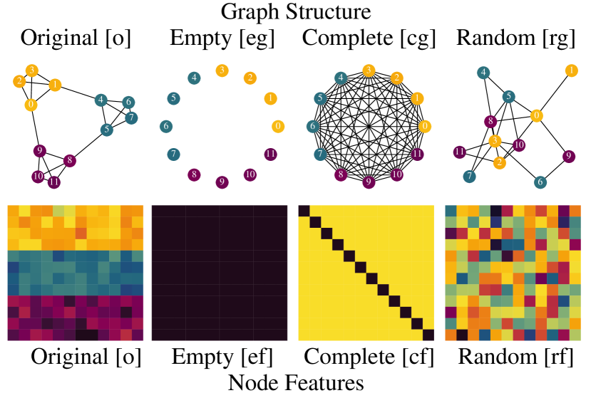
Given an attributed graph , both data modes—i.e., the graph structure and the node features—are naturally associated with metric spaces that encode pairwise distances between nodes (i.e., distance matrices222 Deferring further details to Appendix A, we note that for finite metric spaces, we have , i.e., a finite matrix encoding pairwise distances between elements in . We use in contexts that rely on matrix operations, and to emphasize both the original space and the associated metric. ). In our Rings framework, we modify these metric spaces to reveal information about the quality of graph-learning datasets. This idea is formalized in the notion of mode perturbation.
Definition 2.1 (Mode Perturbation).
A mode perturbation is a map between attributed graphs such that .
This definition is very general, allowing , inter alia, to act on both the graph structure and the node features. For the purposes of understanding the connection between graph structure and node features in graph-learning datasets, however, we focus on mode perturbations that modify either the graph structure or the node features, as illustrated in Figure 1. We start by formalizing our feature perturbations.
Definition 2.2 (Feature Perturbations).
Given an attributed graph on nodes with features , we define:
| [empty features] | ||||
| [complete features] | ||||
| [random features] |
Here, randomizes the features .
We can define a matching set of structural perturbations by modifying our original edge set.
Definition 2.3 (Structural Perturbations).
Given an attributed graph with edge set , we define:
| [empty graph] | ||||
| [complete graph] | ||||
| [random graph] |
Here, randomizes the edge set .
For consistency, we also define the original perturbation [original].
To modify entire collections of graphs, we apply mode perturbations element-wise to all graphs in a given collection.
Definition 2.4 (Dataset Perturbation).
Given a dataset of attributed graphs, a dataset perturbation is given by .
2.2 Performance Separability
By systematically applying mode perturbations to a dataset , we create a set of datasets that contains several different versions of , capturing potentially interesting variation. This variation can be leveraged to investigate the properties derived in Section 1. First addressing P1, we now introduce performance separability as a measure to assess the extent to which both the graph structure and the node features of an attributed graph contain task-relevant information.
Intuitively, given two perturbations , of a dataset as well as a task to be solved on , performance separability measures the distance between performance distributions associated with and . For a formal definition, we need notation describing these distributions.
Definition 2.5 (Tuned Model).
A tuned model is a triple , where represents the dataset and associated task, is the architecture used during training, and denotes the tuned parameters for the specific architecture.
To elucidate the relationship between the graph structure and the node features as it pertains to performance, within Rings, we tune models not only on datasets but also on perturbed datasets .
Definition 2.6 (Tuned Perturbed Model).
For a mode perturbation , denotes a model tuned to solve the task associated with under mode perturbation .
The performance distributions underlying our notion of performance separability can then be defined as follows.
Definition 2.7 (Empirical Performance Distribution).
For a tuned (perturbed) model , given an evaluation metric and a set of initialization conditions , the empirical performance distribution of is the distribution associated with performance measurements
| (1) |
With performance separability, we now enable pairwise comparisons between the performance distributions of models trained and evaluated on distinct perturbations of .
Definition 2.8 (Performance Separability).
Fix a dataset , an evaluation metric , and initialization conditions , and let be mode perturbations. We define the performance separability of and as
| (2) |
where is a method comparing distributions.
In our experiments (Section 4.1), we use the Kolmogorov-Smirnov (KS) statistic with permutation testing to instantiate . This allows us to assess whether the performance distributions associated with and are significantly different. To evaluate P1, we can then interpret a lack of (statistical) performance separability between a model trained on the original data and a model trained on a mode perturbation as evidence that the perturbed mode does not contain (non-redundant) task-relevant information.
2.3 Mode Complementarity
While performance separability allows us to assess dataset quality in a setting similar to traditional model evaluation, it has three main limitations. First, it is task-dependent due to its focus on P1, and thus risks underestimating datasets whose tasks are simply misaligned with the information contained in them. Second, it is measured based on, and hence still to some extent confounded by, model capabilities. And third, it is resource-intensive to compute. To address P2 and forego these limitations, we propose mode complementarity.
Intuitively, as illustrated in Figure 2, for an attributed graph , mode complementarity measures the distance between a metric space constructed from the graph structure and a metric space constructed from the node features. To formalize this, we define a process for constructing metric spaces from both modes in using lift functions.
Definition 2.9 (Metric-Space Construction).
For attributed graph and metric , we construct metric spaces as
| (3) |
i.e., lifts that take in either structure-based distances arising from or feature-based distances arising from and produce a metric space over the node set .
In Rings, we combine these lifts with mode perturbations.
Definition 2.10 (Perturbed Metric Space).
Given an attributed graph and an associated metric , the -perturbed metric space of under is
| (4) |
which we construe as a distance matrix.
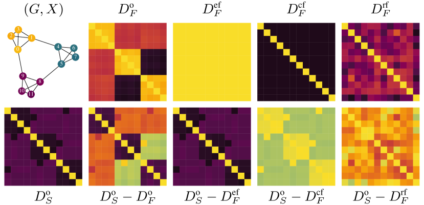
This allows us to assess differences between mode perturbations by comparing metric spaces.
Definition 2.11 (Metric-Space Comparison).
For a fixed set of points and two metrics and , we compare the metric spaces that arise from and by computing the norm of the difference of their matrix representations, i.e.,
| (5) |
With mode complementarity, we then measure the distance between the normalized metric spaces arising from the graph structure and the node features.
Definition 2.12 (Mode Complementarity).
Given an attributed graph with structural metric , derived from , and feature metric , derived from , we define the mode complementarity of as
| (6) |
where is a comparator from Definition 2.11,
| (7) | ||||
| (8) |
using the lifts from Definition 2.9, and we leave (degenerate) zero-diameter spaces unchanged.
Note that since mode complementarity takes an norm of normalized metric spaces, we have by construction. To extend mode complementarity to mode perturbations, we again leverage function composition.
Definition 2.13 (Perturbed Mode Complementarity).
Given an attributed graph and a mode perturbation , the mode complementarity of is
| (9) |
For notational clarity, we use a subscript convention to denote the mode complementarity of under specific mode perturbations, i.e., .
To assess P2, we can interpret high levels of mode complementarity under a given mode perturbation as evidence that, in the metric spaces associated with that perturbation, the graph structure and the features contain complementary information. We can also gain further insights by assessing the differences between mode-complementarity levels across mode perturbations. Depending on the mode perturbations compared, these differences reveal information about the nature of the connection between the graph structure and the node features, or about the diversity present in and .
In Proposition A.10 (Appendix A), we formalize the relationship between empty mode perturbations and what we call self-complementarity, showing that measures the geometric structure of the unperturbed mode. Based on both limiting behaviors of , which correspond to uninformative metric-space structures, we can then define a notion of mode diversity.
Definition 2.14 (Mode Diversity).
Given an attributed graph , the mode diversity of for is
| (10) |
Intuitively, the mode diversity scores the ability of to produce non-trivial geometric structure. Note that implies that or , our canonical uninformative metric spaces.
In our experiments, we instantiate with the Euclidean distance between node features and with a diffusion distance based on the graph structure (explained in Appendix B) to approximate the computations underlying graph-learning methods. We further choose the norm as our comparator, which yields a favorable duality, proved in Appendix A, between empty and complete perturbations.
Theorem 2.15 (Perturbation Duality).
Fix an attributed graph and corresponding distances , for lifting each mode into a metric space. For , Definition 2.12 of yields the equivalence
| (11) |
3 Related Work
Here, we briefly contextualize our contributions, deferring a deeper discussion of related work to Appendix E.
Relating to mode perturbations and performance separability, Errica et al. (2020) create GNN experiments to improve reproducibility, and Bechler-Speicher et al. (2024) show that GNNs use the graph structure even when it is not conducive to a task (i.e., separably outperforms ). Rings is inspired by, and goes beyond, these works, providing a general framework for perturbation-based dataset evaluation.
Connecting with mode complementarity, researchers have been particularly interested in the effects of homo- and heterophily on node-classification performance (Lim et al., 2021; Platonov et al., 2023a, b; Luan et al., 2023). While homophily characterizes the task-dependent relationship between graph structure and node labels, mode complementarity assesses the task-independent relationship between graph structure and node features. For node classification, Dong & Kluger (2023) propose the edge signal-to-noise ratio (ESNR), Qian et al. (2022) develop a subspace alignment measure (SAM), and Thang et al. (2022) analyze relations between node features and graph structure (FvS). However, with mode complementarity, we craft a score that (1) treats graph structure and node features as equal (unlike ESNR), (2) works on graphs without node labels and does not make assumptions about the spaces arising from edge connectivity and node features (unlike SAM, FvS), and (3) specifically informs graph-level learning tasks (unlike all of these works).
| Dataset | Accuracy | AUROC | Structure | Features | Evaluation |
|---|---|---|---|---|---|
| AIDS | cf cg rg o eg rf | cf/cg/rg eg/o rf | uninformative | uninformative | -- |
| COLLAB | o cg/rg eg cf/rf | o cg/rg eg rf cf | informative | informative | ++ |
| DD | rg cg cf eg/o rf | rg cf/cg/eg/o/rf | uninformative | uninformative | -- |
| Enzymes | eg cg/o rg cf rf | eg o cg rg cf rf | uninformative | informative | - |
| IMDB-B | cf/cg/eg/o/rf/rg | o cg eg/rg rf cf | (un)informative | (un)informative | |
| IMDB-M | cg/eg/o/rg cf rf | o cg/eg/rg cf rf | (un)informative | informative | + |
| MUTAG | cf/cg/o/rg eg rf | cf/o cg/eg/rf/rg | (un)informative | uninformative | - |
| MolHIV | o cf/cg/rg rf eg | o cg cf rg eg rf | informative | informative | ++ |
| NCI1 | o cg cf rg eg rf | o cg cf rg eg/rf | informative | informative | ++ |
| Peptides | o cg rg eg cf rf | cg o rg eg cf rf | (un)informative | informative | + |
| Proteins | cf cg/rf eg/o/rg | cf/cg/eg/o/rf/rg | uninformative | uninformative | -- |
| Reddit-B | cf rg o cg eg/rf | rg cf o cg/eg/rf | uninformative | uninformative | -- |
| Reddit-M | rf rg o eg | rg rf o eg | uninformative | uninformative | -- |
4 Experiments
We now demonstrate how to use Rings to evaluate the quality of graph-learning datasets, guided by the principles developed in Section 1. Leveraging our mode-perturbation framework, we explore P1 via performance separability and P2 via mode complementarity, before distilling our observations into an actionable taxonomy of recommendations. For further details and additional results, see Appendix D.333We make all code, data, results, and workflows publicly available. Upon publication, a fully documented reproducibility package will be deposited via Zenodo.
Evaluated Datasets. In our main experiments, we evaluate popular graph-classification datasets: From the life sciences, we select AIDS, ogbg-molhiv (MolHIV), MUTAG, and NCI1 (small molecules), as well as DD, Enzymes, Peptides-func (Peptides), and PROTEINS-full (Proteins) (larger chemical structures). From the social sciences, we take COLLAB, IMDB-B, and IMDB-M (collaboration ego-networks), as well as REDDIT-B and REDDIT-M (online interactions). See Appendix C for details and references.
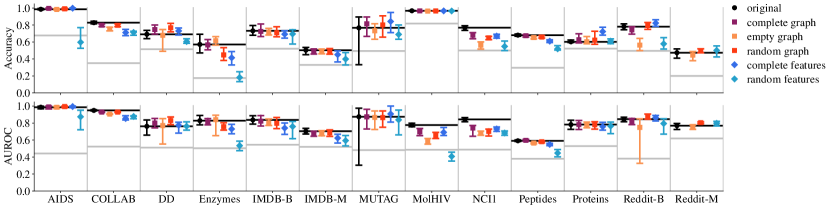
4.1 Performance Separability (P1)
Expectations. (1) For a structure- and feature-based task, the original dataset should separably outperform all other mode perturbations. (2) For a structure-based task, the original dataset should separably outperform all structural perturbations. (3) For a feature-based task, the original dataset should separably outperform all feature perturbations. (4) If the original dataset is separably outperformed by a structural (feature) perturbation, the structural (feature) mode of the dataset is poorly aligned with the task.
Measurement. To evaluate performance separability, we train standard GNN architectures (GAT, GCN, GIN) in the Rings framework on the original and perturbations of our main datasets: {empty, complete, random} graph, and {complete, random} features.444GNNs cannot train with due to uninformative gradients. With the setup described in Appendix Table 4, we tune and evaluate a total of models. Although any GNN architecture could be used to evaluate performance separability within Rings, using standard architectures allows us to focus on dataset evaluation.
For each version of each dataset, we identify the model with the best performance under evaluation metric {accuracy, AUROC} as , using the performance distribution of the top model, , to assess performance separability.
To compare performance distributions, we use permutation tests with the Kolmogorov-Smirnov (KS) statistic, Bonferroni correcting for multiple hypothesis testing within each individual dataset and testing differences for significance at an -level of (see Appendix Tables 10 and 11 for substantively identical results using different setups).
Results. We show the performance of the best GNN models in Figure 3, for the original and mode perturbations over our main datasets and evaluation statistics, and summarize the associated statistical performance-separability results in Table 1. We find that only datasets—COLLAB, MolHIV, and NCI1—satisfy the performance-separability relations expected from structure- and feature-based tasks (with Peptides coming close), whereas datasets—AIDS, DD, Proteins, Reddit-B, and Reddit-M—do not satisfy any separability requirements, highlighting their low quality from the perspective of P1. Among our striking results, the original dataset is separably outperformed by (1) the random-graph perturbation on DD, (2) the empty-graph perturbation on Enzymes, and (3) the complete-features and random-graph perturbations on Reddit-B, indicating that the affected modes are poorly aligned with their current task.
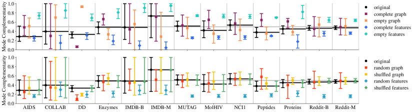
4.2 Mode Complementarity (P2)
Expectations. (1) For a structure- and feature-based task, the original dataset should have high mode complementarity, and both modes should have high mode diversity (indicated by high mode complementarity of the empty and complete perturbations of their dual mode). (2) For a structure-based task, the structural mode should have high mode diversity. (3) For a feature-based task, the feature mode should have high mode diversity. (4) If the original dataset has low mode complementarity, the information contained in structure and features is redundant. (5) If both modes have low mode diversity, the dataset contains little insightful variation.
Measurement. We evaluate mode complementarity for the original as well as fixed and randomized mode perturbations: {complete, empty, random, shuffled} {graph, features} (see Appendix D for detailed descriptions). To measure mode complementarity (and the mode diversity derived from it), for each graph in a given dataset perturbation, we instantiate Definition 2.12 using the Euclidean distance as our feature distance, the diffusion distance (see Appendix B) for a number of diffusion steps as our graph distance, and the norm as our comparator (see Appendix B for examples of other choices).
| Structure | Features | |||||||
|---|---|---|---|---|---|---|---|---|
| Dataset | ||||||||
| AIDS | 0.52 | 0.07 | 0.81 | 0.14 | - | ++ | ||
| COLLAB | 0.30 | 0.20 | 0.27 | 0.24 | - | ++ | - | ++ |
| DD | 0.62 | 0.09 | 0.13 | 0.03 | ++ | - | -- | -- |
| Enzymes | 0.38 | 0.10 | 0.66 | 0.13 | - | - | ++ | |
| IMDB-B | 0.18 | 0.11 | 0.55 | 0.29 | -- | ++ | ||
| IMDB-M | 0.09 | 0.11 | 0.30 | 0.34 | -- | - | ++ | |
| MUTAG | 0.51 | 0.02 | 0.76 | 0.14 | -- | ++ | ||
| MolHIV | 0.55 | 0.05 | 0.69 | 0.21 | -- | ++ | ++ | |
| NCI1 | 0.56 | 0.05 | 0.78 | 0.16 | -- | ++ | ++ | |
| Peptides | 0.61 | 0.01 | 0.71 | 0.23 | ++ | -- | ++ | ++ |
| Proteins | 0.36 | 0.12 | 0.76 | 0.08 | - | ++ | - | |
| Reddit-B | 0.71 | 0.05 | 0.80 | 0.12 | ++ | - | ++ | |
| Reddit-M | 0.72 | 0.03 | 0.85 | 0.11 | ++ | -- | ++ | |
Results. In Figure 4, we show the mean and th percentile intervals of the mode-complementarity distributions at , for the original and the other selected mode perturbations, for each of our main datasets. We observe interesting differences between mode-complementarity profiles across datasets. For example, (1) COLLAB, IMDB-B, and IMDB-M stand out for their large ranges (likely due to their nature as ego-networks); (2) DD attains extreme values with its complete-graph and empty-graph perturbations (likely due to the absence of features in the original dataset, translated into complete-type features by PyTorch-geometric); and (3) Peptides has mode complementarities in the random-graph and the complete-graph perturbations that are noticeably higher than that of the original dataset (possibly related to the presence of long-range connections).
Supplementing Figure 4 with mode-diversity scores in Table 2, we find that feature diversity is more common than structural diversity, and variation in structural diversity is almost always low. Notably, (1) COLLAB, IMDB-B, and IMDB-M, judged favorably or neutral by performance separability, score poorly on structural and feature diversity, suggesting that their tasks may not reveal much information about the power of graph-learning methods; (2) conversely, among the datasets judged problematic by performance separability, DD exhibits high levels of structural diversity, indicating its potential for adequately aligned structural tasks; and (3) Reddit-B and Reddit-M show high levels of structural and feature diversity, indicating untapped potential for graph-learning tasks that are based on both structure and features, as well as high quality from the perspective of P2.
To conclude, we explore the relationship between mean mode complementarity and mean (AUROC) performance across all mode perturbations in Figure 5 (see Appendix Figure 9 and Table 12 for extended results). We find that higher mode complementarity is generally associated with higher performance, with exceptions for some tasks we previously identified as misaligned (DD and Reddit-M). Since evaluating performance separability is comparatively costly, this further underscores the value of mode complementarity as a task-independent diagnostic for graph-learning datasets.
4.3 Dataset Taxonomy
From our observations on performance separability (P1) and mode complementarity (P2), we can distill the following actionable dataset taxonomy, where we note evidence from performance separability () and mode complementarity ():
| Action | Datasets |
|---|---|
| Keep () | MolHIV, NCI1, Peptides |
| Realign () | AIDS, DD, MUTAG, Reddit-B, Reddit-M |
| Deprecate () | Enzymes, Proteins |
| Deprecate () | COLLAB, IMDB-B, IMDB-M |
5 Discussion
Conclusions. We introduced Rings, a principled framework for evaluating graph-learning datasets based on mode perturbations—i.e., controlled changes to their graph structure and node features. In Rings, we developed performance separability as a task-dependent, and mode complementarity as a task-independent measure of dataset quality. Using our framework to categorize popular graph-classification datasets, we identified several benchmarks that require realignment (e.g., by better data modeling) or complete deprecation. While some datasets have been observed to be problematic in prior work, with Rings, we offer a full perturbation-based evaluation pipeline. We designed our initial set of perturbations from a data-centric perspective, but cleverly crafted perturbations could also isolate and confirm the performance separability of any proposed contribution. Thus, we hope that Rings will raise the standard of proof for model-centric evaluation in graph learning as well.
Limitations. Given that message passing is the predominant paradigm in graph learning, our performance-separability experiments target message-passing GNNs, at the exclusion of other architectures. While Rings is a general framework, our current norm-based comparison of metric spaces assumes that nodes and node features are paired. Thus, we presently do not measure aspects like the metric distortion arising from different mappings. Moreover, our notion of mode complementarity is deliberately task-independent and model-agnostic. This allows us to gain insights into datasets, but the inclusion of additional information about models would enable claims about (model, dataset, task) triples.
Future Work. We envision Rings to support the design of better datasets and more challenging tasks for graph learning, and we hope that the community will use our proposed measures to further scrutinize its datasets. Beyond these aspirations, we highlight three concrete avenues for future work. First, although we provide some initial theoretical results on the behavior of perturbed mode complementarity, a comprehensive theoretical analysis of its properties is yet outstanding. Second, while our work focused on graph-level tasks, node-level and edge-level tasks also merit closer inspection, and these tasks might naturally give rise to a localized notion of mode complementarity. And third, studying how mode complementarity changes during training, or how mode-complementarity distributions impact train-eval-test splits, could yield interesting insights into the relationship between mode complementarity and performance.
Impact Statement
With Rings, we introduce a principled data-centric framework for evaluating the quality of graph-learning datasets. We expect our framework to help improve data and evaluation practices in graph learning, enabling the community to focus on datasets that truly require resource-intensive graph-learning approaches via mode complementarity and encouraging greater experimental rigor via performance separability. Thus, we hope to contribute to reducing the environmental impact of the machine-learning community, and to the development of scientifically sound, responsible AI methods.
References
- Agarwal et al. (2023) Agarwal, C., Queen, O., Lakkaraju, H., and Zitnik, M. Evaluating explainability for graph neural networks. Scientific Data, 10(1):144, 2023.
- Akbiyik et al. (2023) Akbiyik, E., Grötschla, F., Egressy, B., and Wattenhofer, R. Graphtester: Exploring theoretical boundaries of gnns on graph datasets. In Data-centric Machine Learning Research (DMLR) Workshop at ICML, 2023.
- Alon & Yahav (2021) Alon, U. and Yahav, E. On the bottleneck of Graph Neural Networks and its practical implications. In International Conference on Learning Representations, 2021.
- Bai & Hancock (2004) Bai, X. and Hancock, E. R. Heat kernels, manifolds and graph embedding. In Structural, Syntactic, and Statistical Pattern Recognition: Joint IAPR International Workshops, pp. 198–206. Springer, 2004.
- Barabási (2016) Barabási, A.-L. Network science. Cambridge University Press, 2016.
- Bechler-Speicher et al. (2024) Bechler-Speicher, M., Amos, I., Gilad-Bachrach, R., and Globerson, A. Graph neural networks use graphs when they shouldn’t. In International Conference on Learning Representations, 2024.
- Biderman & Scheirer (2020) Biderman, S. and Scheirer, W. J. Pitfalls in machine learning research: Reexamining the development cycle. In Proceedings on ”I Can’t Believe It’s Not Better!” at NeurIPS Workshops, volume 137 of Proceedings of Machine Learning Research, pp. 106–117. PMLR, 2020.
- Bonabi Mobaraki & Khan (2023) Bonabi Mobaraki, E. and Khan, A. A demonstration of interpretability methods for Graph Neural Networks. In Proceedings of the 6th Joint Workshop on Graph Data Management Experiences & Systems (GRADES) and Network Data Analytics (NDA), pp. 1–5, 2023.
- Borgwardt et al. (2020) Borgwardt, K., Ghisu, E., Llinares-López, F., O’Bray, L., and Rieck, B. Graph kernels: State-of-the-art and future challenges. Foundations and Trends in Machine Learning, 13(5–6):531–712, 2020.
- Borgwardt et al. (2005) Borgwardt, K. M., Ong, C. S., Schönauer, S., Vishwanathan, S. V. N., Smola, A. J., and Kriegel, H.-P. Protein function prediction via graph kernels. Bioinformatics, 21(1):47–56, 2005.
- Cai & Wang (2018) Cai, C. and Wang, Y. A simple yet effective baseline for non-attributed graph classification. In Representation Learning on Graphs and Manifolds Workshop at ICLR, 2018.
- Chen et al. (2022) Chen, J., Chen, S., Bai, M., Gao, J., Zhang, J., and Pu, J. SA-MLP: Distilling Graph Knowledge from GNNs into Structure-Aware MLP, 2022. arXiv:2210.09609 [cs].
- Chen et al. (2020) Chen, T., Bian, S., and Sun, Y. Are powerful graph neural nets necessary? A dissection on graph classification, 2020. arXiv:1905.04579 [cs].
- Chuang & Jegelka (2022) Chuang, C.-Y. and Jegelka, S. Tree mover’s distance: Bridging graph metrics and stability of graph neural networks. In Advances in Neural Information Processing Systems, pp. 2944–2957, 2022.
- Coifman & Lafon (2006) Coifman, R. R. and Lafon, S. Diffusion maps. Applied and Computational Harmonic Analysis, 21(1):5–30, 2006. Special Issue: Diffusion Maps and Wavelets.
- Debnath et al. (1991) Debnath, A. K., Lopez de Compadre, R. L., Debnath, G., Shusterman, A. J., and Hansch, C. Structure-activity relationship of mutagenic aromatic and heteroaromatic nitro compounds. correlation with molecular orbital energies and hydrophobicity. Journal of Medicinal Chemistry, 34(2):786–797, 1991.
- Di Giovanni et al. (2023) Di Giovanni, F., Giusti, L., Barbero, F., Luise, G., Lio, P., and Bronstein, M. M. On over-squashing in message passing neural networks: The impact of width, depth, and topology. In International Conference on Machine Learning, pp. 7865–7885, 2023.
- Ding & Li (2018) Ding, J. and Li, X. An approach for validating quality of datasets for machine learning. In IEEE International Conference on Big Data, pp. 2795–2803, 2018.
- Dobson & Doig (2003) Dobson, P. D. and Doig, A. J. Distinguishing enzyme structures from non-enzymes without alignments. Journal of Molecular Biology, 330(4):771–783, 2003.
- Dong & Kluger (2023) Dong, M. and Kluger, Y. Towards understanding and reducing graph structural noise for gnns. In International Conference on Machine Learning, pp. 8202–8226, 2023.
- Dwivedi et al. (2022) Dwivedi, V. P., Rampášek, L., Galkin, M., Parviz, A., Wolf, G., Luu, A. T., and Beaini, D. Long range graph benchmark. In Advances in Neural Information Processing Systems, pp. 22326–22340, 2022.
- Errica et al. (2020) Errica, F., Podda, M., Bacciu, D., and Micheli, A. A fair comparison of graph neural networks for graph classification. In International Conference on Learning Representations, 2020.
- Faber et al. (2021) Faber, L., K. Moghaddam, A., and Wattenhofer, R. When comparing to ground truth is wrong: On evaluating GNN explanation methods. In Proceedings of the ACM SIGKDD Conference on Knowledge Discovery & Data Mining, pp. 332–341, 2021.
- Fan et al. (2020) Fan, X., Gong, M., Xie, Y., Jiang, F., and Li, H. Structured self-attention architecture for graph-level representation learning. Pattern Recognition, 100:107084, 2020.
- Fang et al. (2022) Fang, X., Liu, L., Lei, J., He, D., Zhang, S., Zhou, J., Wang, F., Wu, H., and Wang, H. Geometry-enhanced molecular representation learning for property prediction. Nature Machine Intelligence, 4(2):127–134, 2022.
- Fenza et al. (2021) Fenza, G., Gallo, M., Loia, V., Orciuoli, F., and Herrera-Viedma, E. Data set quality in Machine Learning: Consistency measure based on group decision making. Applied Soft Computing, 106:107366, 2021.
- Fey & Lenssen (2019) Fey, M. and Lenssen, J. E. Fast graph representation learning with pytorch geometric. In Representation Learning on Graphs and Manifolds Workshop at ICLR, 2019.
- Gao et al. (2010) Gao, X., Xiao, B., Tao, D., and Li, X. A survey of graph edit distance. Pattern Analysis and Applications, 13(1):113–129, 2010.
- Germani et al. (2023) Germani, E., Fromont, E., Maurel, P., and Maumet, C. The HCP multi-pipeline dataset: An opportunity to investigate analytical variability in fMRI data analysis, 2023. arXiv:2312.14493 [q-bio].
- Han et al. (2023) Han, H., Liu, X., Ma, L., Torkamani, M., Liu, H., Tang, J., and Yamada, M. Structural Fairness-aware Active Learning for Graph Neural Networks. In International Conference on Learning Representations, 2023.
- Hu et al. (2020) Hu, W., Fey, M., Zitnik, M., Dong, Y., Ren, H., Liu, B., Catasta, M., and Leskovec, J. Open graph benchmark: Datasets for machine learning on graphs, 2020.
- Kersting et al. (2016) Kersting, K., Kriege, N. M., Morris, C., Mutzel, P., and Neumann, M. Benchmark data sets for graph kernels, 2016.
- Kipf & Welling (2017) Kipf, T. N. and Welling, M. Semi-supervised classification with graph convolutional networks. In International Conference on Learning Representations, 2017.
- Kriege et al. (2020) Kriege, N. M., Johansson, F. D., and Morris, C. A survey on graph kernels. Applied Network Science, 5(1), 2020.
- Leskovec et al. (2005) Leskovec, J., Kleinberg, J., and Faloutsos, C. Graphs over time: densification laws, shrinking diameters and possible explanations. In Proceedings of the ACM SIGKDD International Conference on Knowledge Discovery in Data Mining, pp. 177–187, 2005.
- Li et al. (2022) Li, P., Yang, Y., Pagnucco, M., and Song, Y. Explainability in graph neural networks: An experimental survey, March 2022. arXiv:2203.09258 [cs].
- Li et al. (2024) Li, Z., Cao, Y., Shuai, K., Miao, Y., and Hwang, K. Rethinking the effectiveness of graph classification datasets in benchmarks for assessing gnns. In Proceedings of the International Joint Conference on Artificial Intelligence, pp. 2144–2152, 2024.
- Lim et al. (2021) Lim, D., Hohne, F., Li, X., Huang, S. L., Gupta, V., Bhalerao, O., and Lim, S. Large scale learning on non-homophilous graphs: New benchmarks and strong simple methods. In Advances in Neural Information Processing Systems, pp. 20887–20902, 2021.
- Limbeck et al. (2024) Limbeck, K., Andreeva, R., Sarkar, R., and Rieck, B. Metric space magnitude for evaluating the diversity of latent representations. In Advances in Neural Information Processing Systems, 2024.
- Lin et al. (2023) Lin, Y., Yang, M., Yu, J., Hu, P., Zhang, C., and Peng, X. Graph matching with bi-level noisy correspondence. In Proceedings of the IEEE/CVF International Conference on Computer Vision, pp. 23362–23371, 2023.
- Luan et al. (2022) Luan, S., Hua, C., Lu, Q., Zhu, J., Zhao, M., Zhang, S., Chang, X., and Precup, D. Revisiting heterophily for graph neural networks. In Advances in Neural Information Processing Systems, 2022.
- Luan et al. (2023) Luan, S., Hua, C., Xu, M., Lu, Q., Zhu, J., Chang, X., Fu, J., Leskovec, J., and Precup, D. When do graph neural networks help with node classification? investigating the homophily principle on node distinguishability. In Advances in Neural Information Processing Systems, 2023.
- Mao et al. (2023) Mao, H., Chen, Z., Jin, W., Han, H., Ma, Y., Zhao, T., Shah, N., and Tang, J. Demystifying structural disparity in graph neural networks: Can one size fit all? In Advances in Neural Information Processing Systems, 2023.
- Mazumder et al. (2023) Mazumder, M., Banbury, C., Yao, X., Karlaš, B., Gaviria Rojas, W., Diamos, S., Diamos, G., He, L., Parrish, A., Kirk, H. R., Quaye, J., Rastogi, C., Kiela, D., Jurado, D., Kanter, D., Mosquera, R., Cukierski, W., Ciro, J., Aroyo, L., Acun, B., Chen, L., Raje, M., Bartolo, M., Eyuboglu, E. S., Ghorbani, A., Goodman, E., Howard, A., Inel, O., Kane, T., Kirkpatrick, C. R., Sculley, D., Kuo, T.-S., Mueller, J. W., Thrush, T., Vanschoren, J., Warren, M., Williams, A., Yeung, S., Ardalani, N., Paritosh, P., Zhang, C., Zou, J. Y., Wu, C.-J., Coleman, C., Ng, A., Mattson, P., and Janapa Reddi, V. DataPerf: Benchmarks for data-centric AI development. In Advances in Neural Information Processing Systems, pp. 5320–5347, 2023.
- Michel et al. (2023) Michel, G., Nikolentzos, G., Lutzeyer, J., and Vazirgiannis, M. Path Neural Networks: Expressive and accurate graph neural networks. In International Conference on Machine Learning, 2023.
- Morris et al. (2020) Morris, C., Kriege, N. M., Bause, F., Kersting, K., Mutzel, P., and Neumann, M. Tudataset: A collection of benchmark datasets for learning with graphs. In Graph Representation Learning and Beyond Workshop at ICML, 2020.
- Morris et al. (2024) Morris, C., Frasca, F., Dym, N., Maron, H., Ceylan, I. I., Levie, R., Lim, D., Bronstein, M. M., Grohe, M., and Jegelka, S. Position: Future directions in the theory of graph machine learning. In International Conference on Machine Learning, 2024.
- Newman (2018) Newman, M. Networks. Oxford University Press, 2018.
- NIH National Cancer Institute (2004) NIH National Cancer Institute. AIDS antiviral screen data, 2004.
- Palowitch et al. (2022) Palowitch, J., Tsitsulin, A., Mayer, B. A., and Perozzi, B. Graphworld: Fake graphs bring real insights for gnns. In Proceedings of the ACM SIGKDD Conference on Knowledge Discovery and Data Mining, pp. 3691–3701, 2022.
- Platonov et al. (2023a) Platonov, O., Kuznedelev, D., Babenko, A., and Prokhorenkova, L. Characterizing graph datasets for node classification: Homophily-heterophily dichotomy and beyond. In Advances in Neural Information Processing Systems, 2023a.
- Platonov et al. (2023b) Platonov, O., Kuznedelev, D., Diskin, M., Babenko, A., and Prokhorenkova, L. A critical look at the evaluation of gnns under heterophily: Are we really making progress? In International Conference on Learning Representations, 2023b.
- Qian et al. (2022) Qian, Y., Expert, P., Rieu, T., Panzarasa, P., and Barahona, M. Quantifying the alignment of graph and features in deep learning. IEEE Trans. Neural Networks Learn. Syst., 33(4):1663–1672, 2022.
- Randić & Klein (1993) Randić, M. and Klein, D. Resistance distance. J. Math. Chem, 12:81–95, 1993.
- Rathee et al. (2022) Rathee, M., Funke, T., Anand, A., and Khosla, M. BAGEL: A Benchmark for Assessing Graph Neural Network Explanations, 2022. arXiv:2206.13983 [cs].
- Riesen & Bunke (2008) Riesen, K. and Bunke, H. IAM graph database repository for graph based pattern recognition and machine learning. In da Vitoria Lobo, N., Kasparis, T., Roli, F., Kwok, J. T., Georgiopoulos, M., Anagnostopoulos, G. C., and Loog, M. (eds.), Structural, Syntactic, and Statistical Pattern Recognition, pp. 287–297, 2008.
- Sanmartín et al. (2022) Sanmartín, E. F., Damrich, S., and Hamprecht, F. A. The algebraic path problem for graph metrics. In International Conference on Machine Learning, 2022.
- Schomburg et al. (2004) Schomburg, I., Chang, A., Ebeling, C., Gremse, M., Heldt, C., Huhn, G., and Schomburg, D. BRENDA, the enzyme database: updates and major new developments. Nucleic Acids Research, 32:D431–D433, 2004.
- Sharma et al. (2024) Sharma, K., Lee, Y.-C., Nambi, S., Salian, A., Shah, S., Kim, S.-W., and Kumar, S. A survey of graph neural networks for social recommender systems. ACM Comput. Surv., 56(10), 2024.
- Shervashidze et al. (2011) Shervashidze, N., Schweitzer, P., van Leeuwen, E. J., Mehlhorn, K., and Borgwardt, K. M. Weisfeiler-lehman graph kernels. Journal of Machine Learning Research, 12(77):2539–2561, 2011.
- Simson et al. (2024) Simson, J., Pfisterer, F., and Kern, C. One model many scores: Using multiverse analysis to prevent fairness hacking and evaluate the influence of model design decisions. In ACM Conference on Fairness, Accountability, and Transparency, pp. 1305–1320, 2024.
- Sonthalia & Gilbert (2020) Sonthalia, R. and Gilbert, A. Tree! I am no tree! I am a low dimensional hyperbolic embedding. Advances in Neural Information Processing Systems, 33:845–856, 2020.
- Stokes et al. (2020) Stokes, J. M., Yang, K., Swanson, K., Jin, W., Cubillos-Ruiz, A., Donghia, N. M., MacNair, C. R., French, S., Carfrae, L. A., Bloom-Ackermann, Z., et al. A deep learning approach to antibiotic discovery. Cell, 180(4):688–702, 2020.
- Taha et al. (2023) Taha, D., Zhao, W., Riestenberg, J. M., and Strube, M. Normed spaces for graph embedding. Transactions on Machine Learning Research, 2023.
- Tang et al. (2023) Tang, J., Zhang, W., Li, J., Zhao, K., Tsung, F., and Li, J. Robust attributed graph alignment via joint structure learning and optimal transport. In International Conference on Data Engineering, pp. 1638–1651, 2023.
- Thang et al. (2022) Thang, D. C., Dat, H. T., Tam, N. T., Jo, J., Hung, N. Q. V., and Aberer, K. Nature vs. nurture: Feature vs. structure for graph neural networks. Pattern Recognition Letters, 159:46–53, 2022.
- Tönshoff et al. (2023) Tönshoff, J., Ritzert, M., Rosenbluth, E., and Grohe, M. Where did the gap go? reassessing the long-range graph benchmark. In Learning on Graphs Conference, 2023.
- Toyokuni & Yamada (2023) Toyokuni, A. and Yamada, M. Structural explanations for Graph Neural Networks using HSIC, February 2023. arXiv:2302.02139 [cs, stat].
- Veličković et al. (2018) Veličković, P., Cucurull, G., Casanova, A., Romero, A., Liò, P., and Bengio, Y. Graph attention networks. In International Conference on Learning Representations, 2018.
- Wale & Karypis (2006) Wale, N. and Karypis, G. Comparison of descriptor spaces for chemical compound retrieval and classification. In International Conference on Data Mining, pp. 678–689, 2006.
- Wang & Shen (2023) Wang, X. and Shen, H.-W. GNNInterpreter: A probabilistic generative model-level explanation for Graph Neural Networks, 2023.
- Wayland et al. (2024) Wayland, J., Coupette, C., and Rieck, B. Mapping the multiverse of latent representations. In International Conference on Machine Learning, 2024.
- Wu et al. (2018) Wu, Z., Ramsundar, B., Feinberg, E. N., Gomes, J., Geniesse, C., Pappu, A. S., Leswing, K., and Pande, V. Moleculenet: a benchmark for molecular machine learning. Chemical science, 9(2):513–530, 2018.
- Xie et al. (2022) Xie, Y., Katariya, S., Tang, X., Huang, E., Rao, N., Subbian, K., and Ji, S. Task-agnostic graph explanations. In Advances in Neural Information Processing Systems, pp. 12027–12039, 2022.
- Xu et al. (2019) Xu, K., Hu, W., Leskovec, J., and Jegelka, S. How powerful are graph neural networks?, 2019. arXiv:1810.00826 [cs].
- Yanardag & Vishwanathan (2015) Yanardag, P. and Vishwanathan, S. Deep graph kernels. In Proceedings of the ACM SIGKDD International Conference on Knowledge Discovery and Data Mining, pp. 1365–1374, 2015.
- Yang et al. (2022) Yang, M., Shen, Y., Li, R., Qi, H., Zhang, Q., and Yin, B. A new perspective on the effects of spectrum in graph neural networks. In International Conference on Machine Learning, pp. 25261–25279, 2022.
- Ying et al. (2018) Ying, R., He, R., Chen, K., Eksombatchai, P., Hamilton, W. L., and Leskovec, J. Graph convolutional neural networks for web-scale recommender systems. In Proceedings of the ACM SIGKDD International Conference on Knowledge Discovery and Data Mining, pp. 974–983, 2018.
- Zambon et al. (2020) Zambon, D., Alippi, C., and Livi, L. Graph random neural features for distance-preserving graph representations. In International Conference on Machine Learning, pp. 10968–10977, 2020.
- Zhao et al. (2020) Zhao, W., Zhou, D., Qiu, X., and Jiang, W. A pipeline for fair comparison of graph neural networks in node classification tasks, 2020. arXiv:2012.10619 [cs].
Appendix
In this appendix, we provide the following supplementary materials.
-
A.
Extended Theory. Definitions, proofs, and results omitted from the main text.
-
B.
Extended Methods. Further details on properties and parts of our Rings pipeline.
-
C.
Extended Dataset Descriptions. Extra details, statistics, and observations on the selected benchmarks.
-
D.
Extended Experiments. Additional details and experiments complementing the discussion in the main paper.
-
E.
Extended Related Work. Discussion of additional related work.
Appendix A Extended Theory
A.1 Metric Spaces
Here, we introduce metric spaces as well as various related notions that improve our understanding of mode complementarity.
Definition A.1 (Metric Space).
A metric space is a tuple that consists of a nonempty set together with a function which satisfies the axioms of a metric, i.e., (i) for all and if and only if , (ii) , and (iii) .
Definition A.2 (Isometry).
Given two metric spaces and , we call a function an isometry if for all .
Definition A.3 (Trivial Metric Space).
We define a trivial metric space as any metric space in the equivalence class of (the single point space) under isometry. In particular, this corresponds to any finite space paired with a metric such that for all . For finite spaces of size , we represent this as the matrix of zeros, .
Definition A.4 (Discrete Metric Space).
A metric space is a discrete metric space if satisfies
| (12) |
For finite spaces of size , we represent this as the matrix of all ones with zero diagonal, . Note that when normalizing non-degenerate spaces to unit diameter, the discrete metric space is one where all non-equal elements are maximally distant from each other, (e.g. a complete graph).
We go from attributed graphs to metric spaces using the lift construction presented in the main paper, restated here for completeness.
See 2.9
A.2 Perturbations
Definition A.5 (Randomization Methods).
Assume we have nodes in . Let be a permutation over an ordered set.
where represents an Erdős–Rényi model, ensuring that each edge is included in independently with probability .
A.3 Complementarity
See 2.10
A.3.1 Comparators
Definition A.6 ( Norm).
For an pairwise distance matrix representing a finite metric space , we define the norm as
| (13) |
See 2.11
See 2.12
A.3.2 Complementarity under Perturbation
See 2.13
Definition A.7 (Complimentarity for Disconnected Graphs).
For a disconnected attributed graph with nodes and connected components, we write as a union . Let denote the subset of features corresponding to nodes in . We define the complementarity for disconnected graphs as the weighted average of the individual component scores
| (14) |
where . Axiom (ii) in Definition A.1, implies that isolated nodes are then assigned a trivial metric space.
Lemma A.8 (Empty Perturbations Lift to Trivial Metric Spaces).
Let be an attributed graph. For any metric , the image of as defined in Definition 2.9 under precomposition with is a trivial metric space, for .
Proof.
() By Definition 2.2, we have . Since is isometric to , any metric must lift to a trivial metric space (by metric-space axiom (ii)).
() For structural metrics , we restrict to those derived from the adjacency matrix of . By convention, is represented as . Hence, an identical argument holds mutatis mutandis, as any metric derived from the zero matrix lifts to a trivial metric space. ∎
Lemma A.9 (Complete Perturbations Lift to Discrete Metric Spaces).
Let be an attributed graph. For any choice of , the image of as defined in Definition 2.9 under precomposition with is a discrete metric space, for .
Proof.
() By Definition 2.2, we have . The identity matrix consists of standard basis vectors (i.e., the one-hot encodings of nodes). We claim that any metric over must be discrete.
Toward a contradiction, assume otherwise. W.l.o.g., suppose the metric space is scaled to unit diameter, implying that there exist such that . Since is uniform, it is invariant under orthogonal transformations, meaning we can permute the standard basis vectors while preserving distances. Thus, for all , we have , contradicting our assumption. Therefore, for all , proving discreteness.
() Here, . The edge set consists of all two-element subsets of , forming a fully connected graph. Similar to Lemma A.8, we restrict to metrics defined over the adjacency matrix of . By construction, , which has the same structure as under the isometry . Since all elements are maximally distant, any metric must lift to a discrete space. ∎
See 2.15
Proof.
The justifications for the above steps are as follows:
-
•
Line 1: Definition 2.13.
-
•
Line 2: Lemma A.9.
-
•
Line 3: Definition 2.11.
-
•
Line 4: Definition A.6.
-
•
Line 5: Unit-diameter assumption: .
-
•
Line 6: Axiom (ii) of Definition A.1.
-
•
Line 7: Definition A.6.
-
•
Line 8: Definition of and Lemma A.8.
Note that a symmetrical argument can be applied to . This concludes the proof.
See 2.14
Proposition A.10 (Self-Complementarity).
Let and be metrics over the modes of an attributed graph . We define and as dual pairs that can be used to analyze the self-complementarity of a single mode. By construction, for , we have:
| (15) |
Thus, the complementarity under empty perturbations, , measures the internal structure of the nonzero dual mode:
| (16) |
Due to the normalization, we obtain . The limiting behavior of , then, provides insights into the underlying metric structure of the dual mode:
-
(1)
If , then for all .
-
(2)
If , then for all .
Appendix B Extended Methods
B.1 Mode Complementarity
The perturbations introduced with our Rings framework are specifically designed to disentangle the relationship between the structural mode and the feature mode of . Unlike existing methods, Rings allows us to leverage the relationships both between and within individual modes:
Here, all arrows indicate the calculation of potential similarity measures. Solid arrows describe settings for which similarity measures are already known, such as graph kernels (Borgwardt et al., 2020; Kriege et al., 2020), graph edit distances (Gao et al., 2010), or distance metrics on . The dashed arrows show our ability to study complementarity and self-complementarity using metric spaces and principled mode perturbations.
B.2 Metric Choices
As outlined in Section 2.3, we would like to understand, for a given attributed graph the complementarity between the information in the graph structure and the node features. Thus, we use to score the difference in geometric information contained in the two modes. As per Definition 2.12, this requires a choice of a structural metric () and a feature metric (), which facilitate lifting the modes into a metric space.
While our experimental results are based on diffusion distance as our structural distance metric () and Euclidean distance in as our feature-based distance metric (), it is worth noting that the Rings framework generalizes to other distance metrics. Below, we define the diffusion distance and Euclidean distance, as well as several other distance metrics suitable for the Rings framework. To build intuition, we additionally depict the behavior of different graph-distance candidates under edge addition on toy data in Figure 6 and illustrate the interplay between metric choices for the real-world Peptides dataset in Figure 7.

B.2.1 Structural Metrics
Disconnected Graphs
Here we define the metrics we use to lift a graph structure into a metric space. Although common practice assigns an infinite distance between unconnected nodes, due to our treatment of disconnected graphs in Definition A.7, we only lift metric spaces within a connected component. Our treatment of isolated nodes assigns trivial metric spaces to each node, and their union we also treat as trivial as seen in Lemma A.8.
Definition B.1 (Laplacian Variants).
We define the Laplacian of as
| (17) |
where is the adjacency matrix specified by , and is the degree matrix. We also define a normalized Laplacian
| (18) |
where .
Definition B.2 (Diffusion Distance [] (Coifman & Lafon, 2006)).
We define our distance over for diffusion steps as
| (19) |
where is a family of diffusion maps computed from the spectrum of . In particular,
where are the eigenvalue and eigenvector of .
Definition B.3 (Heat-Kernel Distance (Bai & Hancock, 2004)).
To compute the heat-kernel distance between nodes in a graph , we take the spectral decomposition of as
| (20) |
where is the diagonal matrix with ordered eigenvalues and is the matrix with columns corresponding to the ordered eigenvectors. The heat equation associated with the graph Laplacian, written in terms of the heat kernel and time , is defined as
Finally, the heat-kernel distance between nodes and at time is then computed as:
| (21) |
Definition B.4 (Resistance Distance (Randić & Klein, 1993)).
Given a graph with nodes, the resistance distance between nodes and is given as:
| (22) |
where
with denoting the Moore-Penrose pseudoinverse.
Definition B.5 (Shortest-Path Distance).
For a graph , we define the shortest-path distance between two nodes as the minimum number of edges in any path between and .
B.2.2 Feature Metrics
Definition B.6 (Euclidean Distance []).
Given our feature space , let be two arbitrary feature vectors. Then the Euclidean distance (also known as the L2 norm) between and is defined as
| (23) |
Definition B.7 (Cosine Distance).
Given a feature space , let be two arbitrary feature vectors. Then the cosine distance between and is defined as
| (24) |
where is the dot product of and , and is the L2 norm of .
Appendix C Extended Dataset Descriptions
As we seek to evaluate the datasets in their capacity as graph-learning benchmarks, the formulation and properties of these datasets are worth detailed discussion. We summarize the basic statistics of these datasets in Table 3 and now describe the semantics and special characteristics of each dataset in turn.
| Dataset | |||||||||||||
|---|---|---|---|---|---|---|---|---|---|---|---|---|---|
| AIDS | 2000 | 15.69 | 13.69 | 32.39 | 30.02 | 2.01 | 0.20 | 0.19 | 0.08 | 0.29 | 0.08 | 0.28 | 0.06 |
| COLLAB | 5000 | 74.49 | 62.31 | 4914.43 | 12879.12 | 37.37 | 43.97 | 0.51 | 0.30 | 0.40 | 0.27 | 0.64 | 0.21 |
| DD | 1178 | 284.32 | 272.12 | 1431.32 | 1388.40 | 4.98 | 0.59 | 0.03 | 0.02 | 0.33 | 0.04 | 0.80 | 0.06 |
| Enzymes | 600 | 32.63 | 15.29 | 124.27 | 51.04 | 3.86 | 0.49 | 0.16 | 0.11 | 0.49 | 0.07 | 0.26 | 0.05 |
| IMDB-B | 1000 | 19.77 | 10.06 | 193.06 | 211.31 | 8.89 | 5.05 | 0.52 | 0.24 | 0.49 | 0.23 | 0.53 | 0.20 |
| IMDB-M | 1500 | 13.00 | 8.53 | 131.87 | 221.63 | 8.10 | 4.82 | 0.77 | 0.26 | 0.73 | 0.30 | 0.75 | 0.28 |
| MUTAG | 188 | 17.93 | 4.59 | 39.59 | 11.40 | 2.19 | 0.11 | 0.14 | 0.04 | 0.51 | 0.07 | 0.48 | 0.02 |
| MolHIV | 41127 | 25.51 | 12.11 | 54.94 | 26.43 | 2.14 | 0.11 | 0.10 | 0.04 | 0.42 | 0.11 | 0.33 | 0.08 |
| NCI1 | 4110 | 29.87 | 13.57 | 64.60 | 29.87 | 2.16 | 0.11 | 0.09 | 0.04 | 0.54 | 0.05 | 0.51 | 0.03 |
| Peptides | 10873 | 151.54 | 84.10 | 308.54 | 171.99 | 2.03 | 0.04 | 0.02 | 0.02 | 0.38 | 0.09 | 0.26 | 0.04 |
| Proteins | 1113 | 39.06 | 45.78 | 145.63 | 169.27 | 3.73 | 0.42 | 0.21 | 0.20 | 0.45 | 0.04 | 0.26 | 0.06 |
| Reddit-B | 2000 | 429.63 | 554.20 | 995.51 | 1246.29 | 2.34 | 0.31 | 0.02 | 0.03 | 0.47 | 0.03 | 0.45 | 0.08 |
| Reddit-M | 4999 | 508.52 | 452.62 | 1189.75 | 1133.65 | 2.25 | 0.20 | 0.01 | 0.01 | 0.48 | 0.02 | 0.43 | 0.07 |
C.1 Social Sciences
C.1.1 Professional Collaborations
In professional collaboration networks, nodes represent individuals and edges connect those with a direct working relationship.
COLLAB (Yanardag & Vishwanathan, 2015) is a dataset of physics collaboration networks, where nodes represent physics researchers and edges connect co-authors. Graphs are constructed as ego-networks around a central physics researcher, whose subfield (high energy physics, condensed matter physics, or astrophysics) acts as the classification for the graph as a whole. The data to build these graphs is drawn from three public collaboration datasets based on the arXiv (Leskovec et al., 2005).
Following a similar construction, the IMDB (Yanardag & Vishwanathan, 2015) datasets capture collaboration in movies. Graphs represent the ego-networks of actors and actresses, and edges connect those who appear in the same movie. The graph is classified according to the genre of the movies from which these shared acting credits are pulled. The task is to predict this genre, a binary classification between Action and Comedy in IMDB-B, and a multi-class classification between Comedy, Romance, and Sci-Fi in IMDB-M. (Note that genres are engineered to be mutually exclusive.) As one might expect, we note in Figure 3 the lower GNN performance for IMDB-M as compared to IMDB-B, suggesting that the multi-class graph classification is a more challenging task.
COLLAB and IMDB datasets share two notable features that distinguish them from the remaining datasets. First, graphs are constructed as ego-networks. This means that they have a diameter of at most two, in stark contrast to more structurally complex graphs from other datasets. This lends insight into why COLLAB and IMDB are classified as having low structural diversity (see Table 2). Second, node features are constructed from the node degree, rather than providing new information independent of graph structure. Thus, the low diversity scores with high variability that we see in Table 2 are simply a reflection of the node-degree distributions in these datasets.
C.1.2 Social Media
We study two graph-learning datasets with origins in social media: REDDIT-B and REDDIT-M (Yanardag & Vishwanathan, 2015).
In the these datasets, a graph models a thread lifted from a subreddit (i.e., a specific discussion community). Nodes represent Reddit users and edges connect users if at least one of them has replied to a comment made by the other (i.e., the users have had at least one interaction). Like COLLAB and IMDB, node features are constructed from the node degree. However, the REDDIT datasets score better on both structural and feature diversity (see Table 2). REDDIT’s higher structural diversity reflects the fact that its graphs are not ego-networks. Its more complex graph structures also account for the higher diversity in node features (i.e., node degrees).
The REDDIT-B dataset draws from four popular subreddits, two of which follow a Q&A structure (IAmA, AskReddit) and two of which are discussion-based (TrollXChromosomes, atheism). The task is to classify graphs based on these two styles of thread. REDDIT-M graphs are drawn from five subreddits, which also act as the graph class (worldnews, videos, AdviceAnimals, aww and mildlyinteresting).
C.2 Life Sciences
C.2.1 Molecules and Compounds
Graphs provide an elegant way to model molecules, with nodes representing atoms and edges representing the chemical bonds between them.
The AIDS dataset (Riesen & Bunke, 2008), for example, is built from a repository of molecules in the AIDS Antiviral Screen Database of Active Compounds (NIH National Cancer Institute, 2004). Nodes have four features (Morris et al., 2020), most notably their unique atomic number. This is a binary-classification dataset in which molecules are classified by whether or not they demonstrate activity against the HIV virus. Among the 2 000 graphs in this dataset, note that the two classes are imbalanced: there are four times as many inactive molecules (1 600) as active (400). The MolHIV (ogbg-molhiv) dataset, introduced by the Open Graph Benchmark (Hu et al., 2020) with over 40,000 molecules from MoleculeNet (Wu et al., 2018), proposes a similar task. Like AIDS, MolHIV classifies molecules into two classes based on their ability or inability to suppress the HIV virus. However, nodes in the MolHIV dataset have features (compared to in AIDS), including atomic number, chirality, and formal charge.
MUTAG (Debnath et al., 1991) is a relatively small molecular dataset compared with its peers, having only graphs (Morris et al., 2020). However, it does have a similar number of node features (). Graphs represent aromatic or heteroaromatic nitro compounds, which are divided into two classes by their mutagenicity towards the bacterium S. typhimurium, i.e. their ability to cause mutations its DNA. While small, the dataset contains an “extremely broad range of molecular structures” (Debnath et al., 1991), which we see reflected in a decent structural-diversity score in Table 2.
When introducing the dataset, Debnath et al. (1991) found that both specific sets of atoms and certain structural features (namely the presence of or more fused rings), tended to be fairly well correlated with increased mutagenicity. This biologically supports that both modes could be informative, which is generally encouraging for graph-learning datasets. Thus, although we do not observe the desired performance separability in Figure 3, we cannot rule out that MUTAG could be a good benchmark, given a different task.
NCI1 (Wale & Karypis, 2006) is a binary-classification dataset that splits molecules into two classes based on whether or not they have an inhibitary effect on the growth of human lung-cancer cell lines. Nodes have features, a significant step up from other molecular datasets, which is reflected in the richness of NCI1’s feature diversity (see Table 2).
C.2.2 Larger Chemical Structures
The Peptides (Peptides-func) dataset (Dwivedi et al., 2022) classifies peptides by their function. Each graph represents a peptide (i.e., a 1D amino acid chain), with nodes representing heavy (non-hydrogen) atoms and edges representing the bonds between them. Peptides is a multi-label-classification dataset, meaning that each peptide may belong to more than one of the function classes (Antibacterial, Antiviral, cell-cell communication, etc.), with the average being 1.65 classes per peptide. Given the complexity of this task, it is perhaps unsurprising to notice that our tuned GNNs achieve the lowest AURUC on this dataset (see Figure 3).
DD, ENZYMES, and Proteins (Proteins-full) are all protein datasets. Each dataset draws upon the framework introduced by (Borgwardt et al., 2005) to model 3D structures of folded proteins as graphs, with nodes representing amino acids and edges connecting amino acids within a given proximity measured in Angstroms. Both the Proteins-full database introduced by (Borgwardt et al., 2005) and the DD database used by (Shervashidze et al., 2011) are based on data from Dobson & Doig (2003), which classifies proteins as either enzymes () or non-enzymes (). Thus, these two datasets are binary-classification datasets.
Proteins-full only uses of the proteins from Dobson & Doig (2003) but encodes descriptive node features, whereas DD encodes none (Kersting et al., 2016; Morris et al., 2020). This distinction is responsible for Proteins-full’s drastically higher feature diversity score and standard deviation, as seen in Table 2.
ENZYMES (Borgwardt et al., 2005) introduces a multi-class classification task on enzymes. Graphs represent enzymes from the BRENDA database (Schomburg et al., 2004), which are classified according to the Enzyme Commission top-level enzyme classes (EC classes). The dataset is roughly half the size of DD and Proteins-full, with only enzymes ( from each class). There are node features, producing the high feature diversity observed in Table 2.
C.3 Further Information
Several efforts have been made to consolidate information about the aforementioned datasets and their peers. In particular, we direct the interested reader to the TUDataset documentation (Morris et al., 2020), TU Dortmund’s Benchmark Data Sets for Graph Kernels (Kersting et al., 2016), and PyTorch Geometric (Fey & Lenssen, 2019).
Appendix D Extended Experiments
D.1 Extended Setup
With the Rings framework, we introduce principled perturbations to graph learning datasets that allow us to evaluate the extent to which graph structure and node features are leveraged in a given task (performance separability) and to what extent the information in these modes is complementary or redundant (mode complementarity). We do so with a series of experiments, which we expand upon below.
| Aspect | Details |
|---|---|
| Architectures | GAT, GCN, GIN |
| Mode Perturbations | |
| Tuning Strategy | 5-fold CV 64 consistent |
| for each | |
| Selection Metric | Validation AUROC |
| Evaluation Strategy | Tuned model re-trained |
| on distinct CV splits and random seeds, | |
| then evaluated on ’s test set. |
| Parameter | Values |
|---|---|
| Activation | ReLU |
| Batch Size | {64, 128} |
| Dropout | {0.1, 0.5} |
| Fold | {0, 1, 2, 3, 4} |
| Hidden Dim | {128, 256} |
| Learning Rate (LR) | {0.01, 0.001} |
| Max Epochs | 200 |
| Normalization | Batch |
| Num Layers | 3 |
| Optimizer | Adam |
| Readout | Sum |
| Seed | {0, 42} |
| Weight Decay | {0.0005, 0.005} |
D.2 Extended Performance Separability
We begin with a note on the chosen GNN architectures, before examining and supplementing the results of our performance separability evaluations.
D.2.1 A Note on GNN Architectures
By far the most computationally expensive part of our experiments is tuning GNNs. While variation in the GNN models is desirable to ensure that our results are not overly dependent on a specific architecture, we were limited in the number of GNN models that we could train and evaluate over all of our datasets and their perturbations. As our goal is to evaluate the intrinsic quality of datasets as graph-learning benchmarks, we are more concerned with consistency across experiments than with using the newest methods, especially given finite computational resources.
In accordance with other “evaluation of evaluations” studies (Bechler-Speicher et al., 2024; Li et al., 2024), we opted to use several of the most common GNN architectures, namely GCN (Kipf & Welling, 2017), GAT (Veličković et al., 2018), and GIN (Xu et al., 2019). As noted by Li et al. (2024), GCN and GIN provide a good contrast in methodology, with GCN taking a spectral approach and GIN taking a spatial approach.
For each (dataset, perturbation, architecture) triple, we tune the GNN hyperparameters as outlined in Table 4, using the tuning parameters () stated in Table 5. The mean and standard deviation of accuracy and AUROC for our tuned models are tabulated in Table 6 and Table 7, respectively.
| Dataset | o | o | cg | cg | eg | eg | rg | rg | cf | cf | rf | rf | |
|---|---|---|---|---|---|---|---|---|---|---|---|---|---|
| AIDS | GAT | 0.980 | 0.006 | 0.968 | 0.017 | 0.977 | 0.007 | 0.968 | 0.011 | 0.998 | 0.002 | 0.320 | 0.075 |
| GCN | 0.982 | 0.005 | 0.950 | 0.016 | 0.983 | 0.004 | 0.837 | 0.058 | 0.997 | 0.003 | 0.340 | 0.051 | |
| GIN | 0.986 | 0.004 | 0.996 | 0.003 | 0.981 | 0.005 | 0.991 | 0.004 | 0.998 | 0.003 | 0.597 | 0.052 | |
| COLLAB | GAT | 0.821 | 0.009 | 0.798 | 0.008 | 0.753 | 0.013 | 0.797 | 0.009 | 0.675 | 0.019 | 0.647 | 0.013 |
| GCN | 0.827 | 0.009 | 0.798 | 0.008 | 0.753 | 0.014 | 0.790 | 0.009 | 0.705 | 0.018 | 0.712 | 0.012 | |
| GIN | 0.797 | 0.021 | 0.768 | 0.028 | 0.743 | 0.015 | 0.769 | 0.022 | 0.712 | 0.018 | 0.696 | 0.021 | |
| DD | GAT | 0.580 | 0.085 | 0.747 | 0.029 | 0.598 | 0.086 | 0.696 | 0.090 | 0.721 | 0.045 | 0.579 | 0.049 |
| GCN | 0.691 | 0.028 | 0.746 | 0.032 | 0.678 | 0.057 | 0.767 | 0.025 | 0.731 | 0.022 | 0.606 | 0.014 | |
| GIN | 0.683 | 0.037 | 0.601 | 0.073 | 0.670 | 0.050 | 0.594 | 0.074 | 0.710 | 0.030 | 0.597 | 0.018 | |
| Enzymes | GAT | 0.470 | 0.054 | 0.415 | 0.065 | 0.530 | 0.044 | 0.406 | 0.053 | 0.414 | 0.044 | 0.173 | 0.032 |
| GCN | 0.563 | 0.036 | 0.566 | 0.033 | 0.615 | 0.029 | 0.448 | 0.041 | 0.410 | 0.038 | 0.169 | 0.035 | |
| GIN | 0.572 | 0.058 | 0.332 | 0.068 | 0.607 | 0.094 | 0.338 | 0.062 | 0.400 | 0.048 | 0.182 | 0.029 | |
| IMDB-B | GAT | 0.719 | 0.027 | 0.725 | 0.042 | 0.712 | 0.024 | 0.699 | 0.029 | 0.649 | 0.035 | 0.540 | 0.032 |
| GCN | 0.732 | 0.033 | 0.719 | 0.039 | 0.716 | 0.022 | 0.704 | 0.025 | 0.692 | 0.024 | 0.606 | 0.034 | |
| GIN | 0.724 | 0.034 | 0.706 | 0.034 | 0.704 | 0.025 | 0.710 | 0.029 | 0.688 | 0.034 | 0.695 | 0.045 | |
| IMDB-M | GAT | 0.493 | 0.023 | 0.489 | 0.017 | 0.478 | 0.028 | 0.489 | 0.019 | 0.431 | 0.029 | 0.349 | 0.026 |
| GCN | 0.504 | 0.021 | 0.484 | 0.018 | 0.496 | 0.015 | 0.487 | 0.018 | 0.451 | 0.026 | 0.383 | 0.021 | |
| GIN | 0.475 | 0.047 | 0.476 | 0.032 | 0.484 | 0.025 | 0.489 | 0.019 | 0.452 | 0.031 | 0.398 | 0.041 | |
| MUTAG | GAT | 0.707 | 0.051 | 0.677 | 0.083 | 0.667 | 0.042 | 0.688 | 0.038 | 0.755 | 0.087 | 0.624 | 0.079 |
| GCN | 0.718 | 0.044 | 0.710 | 0.081 | 0.733 | 0.061 | 0.756 | 0.061 | 0.842 | 0.075 | 0.625 | 0.059 | |
| GIN | 0.767 | 0.140 | 0.814 | 0.068 | 0.707 | 0.056 | 0.801 | 0.068 | 0.821 | 0.078 | 0.689 | 0.042 | |
| MolHIV | GAT | 0.962 | 0.003 | 0.653 | 0.151 | 0.964 | 0.001 | 0.955 | 0.005 | 0.966 | 0.001 | 0.965 | 0.001 |
| GCN | 0.967 | 0.002 | 0.966 | 0.001 | 0.963 | 0.002 | 0.966 | 0.001 | 0.965 | 0.001 | 0.965 | 0.001 | |
| GIN | 0.968 | 0.002 | 0.965 | 0.001 | 0.963 | 0.001 | 0.965 | 0.002 | 0.965 | 0.001 | 0.965 | 0.001 | |
| NCI1 | GAT | 0.562 | 0.056 | 0.580 | 0.037 | 0.506 | 0.004 | 0.575 | 0.031 | 0.666 | 0.014 | 0.500 | 0.001 |
| GCN | 0.720 | 0.019 | 0.664 | 0.012 | 0.563 | 0.022 | 0.639 | 0.014 | 0.670 | 0.013 | 0.501 | 0.002 | |
| GIN | 0.769 | 0.016 | 0.681 | 0.030 | 0.561 | 0.019 | 0.648 | 0.011 | 0.667 | 0.015 | 0.548 | 0.039 | |
| Peptides | GAT | 0.604 | 0.104 | 0.297 | 0.155 | 0.418 | 0.222 | 0.410 | 0.164 | 0.582 | 0.014 | 0.515 | 0.000 |
| GCN | 0.671 | 0.006 | 0.673 | 0.008 | 0.651 | 0.007 | 0.633 | 0.013 | 0.610 | 0.010 | 0.515 | 0.000 | |
| GIN | 0.681 | 0.008 | 0.661 | 0.008 | 0.653 | 0.008 | 0.659 | 0.007 | 0.570 | 0.046 | 0.520 | 0.014 | |
| Proteins | GAT | 0.600 | 0.015 | 0.620 | 0.038 | 0.599 | 0.007 | 0.614 | 0.034 | 0.723 | 0.024 | 0.610 | 0.015 |
| GCN | 0.597 | 0.006 | 0.627 | 0.033 | 0.603 | 0.023 | 0.595 | 0.006 | 0.714 | 0.024 | 0.607 | 0.011 | |
| GIN | 0.603 | 0.011 | 0.601 | 0.049 | 0.601 | 0.012 | 0.622 | 0.046 | 0.701 | 0.034 | 0.606 | 0.011 | |
| Reddit-B | GAT | 0.730 | 0.029 | 0.595 | 0.080 | 0.520 | 0.032 | 0.678 | 0.061 | 0.700 | 0.064 | 0.518 | 0.024 |
| GCN | 0.781 | 0.018 | 0.742 | 0.026 | 0.540 | 0.050 | 0.794 | 0.023 | 0.823 | 0.019 | 0.580 | 0.039 | |
| GIN | 0.699 | 0.109 | 0.564 | 0.038 | 0.693 | 0.107 | 0.699 | 0.085 | 0.561 | 0.087 | |||
| Reddit-M | GAT | 0.422 | 0.021 | 0.331 | 0.060 | 0.307 | 0.097 | 0.284 | 0.039 | ||||
| GCN | 0.472 | 0.017 | 0.446 | 0.026 | 0.497 | 0.013 | 0.454 | 0.018 | |||||
| GIN | 0.474 | 0.027 | 0.420 | 0.041 | 0.422 | 0.051 | 0.501 | 0.042 |
| Dataset | o | o | cg | cg | eg | eg | rg | rg | cf | cf | rf | rf | |
|---|---|---|---|---|---|---|---|---|---|---|---|---|---|
| AIDS | GAT | 0.984 | 0.012 | 0.985 | 0.011 | 0.981 | 0.010 | 0.984 | 0.010 | 0.994 | 0.008 | 0.829 | 0.141 |
| GCN | 0.986 | 0.010 | 0.954 | 0.020 | 0.986 | 0.009 | 0.982 | 0.011 | 0.995 | 0.006 | 0.874 | 0.055 | |
| GIN | 0.987 | 0.011 | 0.991 | 0.011 | 0.984 | 0.010 | 0.994 | 0.006 | 0.994 | 0.008 | 0.813 | 0.160 | |
| COLLAB | GAT | 0.945 | 0.005 | 0.929 | 0.004 | 0.905 | 0.003 | 0.929 | 0.003 | 0.828 | 0.015 | 0.824 | 0.010 |
| GCN | 0.949 | 0.004 | 0.929 | 0.003 | 0.905 | 0.003 | 0.926 | 0.003 | 0.847 | 0.013 | 0.877 | 0.008 | |
| GIN | 0.926 | 0.022 | 0.906 | 0.034 | 0.897 | 0.007 | 0.908 | 0.023 | 0.855 | 0.013 | 0.858 | 0.017 | |
| DD | GAT | 0.642 | 0.163 | 0.801 | 0.029 | 0.720 | 0.198 | 0.766 | 0.126 | 0.773 | 0.030 | 0.703 | 0.113 |
| GCN | 0.749 | 0.028 | 0.797 | 0.034 | 0.770 | 0.072 | 0.830 | 0.026 | 0.763 | 0.021 | 0.762 | 0.024 | |
| GIN | 0.762 | 0.053 | 0.755 | 0.120 | 0.769 | 0.044 | 0.733 | 0.130 | 0.751 | 0.038 | 0.747 | 0.059 | |
| Enzymes | GAT | 0.767 | 0.033 | 0.729 | 0.044 | 0.797 | 0.022 | 0.729 | 0.033 | 0.730 | 0.028 | 0.513 | 0.032 |
| GCN | 0.816 | 0.017 | 0.811 | 0.020 | 0.829 | 0.017 | 0.758 | 0.025 | 0.718 | 0.025 | 0.505 | 0.030 | |
| GIN | 0.828 | 0.032 | 0.671 | 0.047 | 0.840 | 0.053 | 0.682 | 0.044 | 0.722 | 0.033 | 0.534 | 0.031 | |
| IMDB-B | GAT | 0.811 | 0.030 | 0.822 | 0.036 | 0.803 | 0.025 | 0.791 | 0.026 | 0.694 | 0.035 | 0.561 | 0.037 |
| GCN | 0.837 | 0.028 | 0.821 | 0.037 | 0.803 | 0.023 | 0.793 | 0.026 | 0.741 | 0.037 | 0.644 | 0.042 | |
| GIN | 0.811 | 0.040 | 0.795 | 0.039 | 0.789 | 0.026 | 0.798 | 0.030 | 0.742 | 0.036 | 0.759 | 0.053 | |
| IMDB-M | GAT | 0.687 | 0.024 | 0.673 | 0.019 | 0.668 | 0.022 | 0.683 | 0.020 | 0.597 | 0.022 | 0.527 | 0.023 |
| GCN | 0.704 | 0.020 | 0.668 | 0.019 | 0.684 | 0.021 | 0.679 | 0.020 | 0.623 | 0.029 | 0.566 | 0.019 | |
| GIN | 0.671 | 0.037 | 0.658 | 0.027 | 0.674 | 0.018 | 0.677 | 0.019 | 0.623 | 0.028 | 0.594 | 0.036 | |
| MUTAG | GAT | 0.836 | 0.063 | 0.761 | 0.119 | 0.867 | 0.081 | 0.840 | 0.062 | 0.898 | 0.062 | 0.618 | 0.110 |
| GCN | 0.846 | 0.048 | 0.744 | 0.075 | 0.814 | 0.068 | 0.825 | 0.058 | 0.908 | 0.066 | 0.585 | 0.092 | |
| GIN | 0.874 | 0.155 | 0.874 | 0.067 | 0.814 | 0.075 | 0.865 | 0.048 | 0.882 | 0.078 | 0.838 | 0.079 | |
| MolHIV | GAT | 0.689 | 0.016 | 0.633 | 0.048 | 0.452 | 0.022 | 0.654 | 0.019 | 0.685 | 0.023 | 0.359 | 0.017 |
| GCN | 0.726 | 0.014 | 0.630 | 0.011 | 0.588 | 0.007 | 0.645 | 0.016 | 0.691 | 0.028 | 0.361 | 0.018 | |
| GIN | 0.777 | 0.013 | 0.696 | 0.022 | 0.590 | 0.019 | 0.646 | 0.023 | 0.670 | 0.028 | 0.409 | 0.028 | |
| NCI1 | GAT | 0.572 | 0.135 | 0.680 | 0.051 | 0.679 | 0.017 | 0.664 | 0.065 | 0.727 | 0.016 | 0.683 | 0.016 |
| GCN | 0.797 | 0.017 | 0.735 | 0.013 | 0.647 | 0.029 | 0.685 | 0.017 | 0.731 | 0.017 | 0.648 | 0.022 | |
| GIN | 0.843 | 0.014 | 0.741 | 0.031 | 0.640 | 0.034 | 0.701 | 0.022 | 0.722 | 0.016 | 0.656 | 0.024 | |
| Peptides | GAT | 0.553 | 0.042 | 0.401 | 0.069 | 0.444 | 0.093 | 0.446 | 0.065 | 0.548 | 0.006 | 0.401 | 0.006 |
| GCN | 0.582 | 0.004 | 0.596 | 0.006 | 0.561 | 0.008 | 0.580 | 0.006 | 0.549 | 0.008 | 0.400 | 0.007 | |
| GIN | 0.591 | 0.005 | 0.571 | 0.012 | 0.565 | 0.004 | 0.573 | 0.007 | 0.536 | 0.008 | 0.447 | 0.027 | |
| Proteins | GAT | 0.775 | 0.018 | 0.752 | 0.042 | 0.786 | 0.016 | 0.764 | 0.035 | 0.758 | 0.022 | 0.720 | 0.030 |
| GCN | 0.782 | 0.021 | 0.782 | 0.027 | 0.773 | 0.028 | 0.780 | 0.024 | 0.758 | 0.027 | 0.730 | 0.031 | |
| GIN | 0.782 | 0.028 | 0.735 | 0.092 | 0.736 | 0.061 | 0.751 | 0.046 | 0.742 | 0.034 | 0.765 | 0.032 | |
| Reddit-B | GAT | 0.798 | 0.022 | 0.763 | 0.049 | 0.749 | 0.148 | 0.740 | 0.088 | 0.721 | 0.082 | 0.624 | 0.178 |
| GCN | 0.846 | 0.014 | 0.817 | 0.019 | 0.639 | 0.195 | 0.875 | 0.016 | 0.862 | 0.015 | 0.797 | 0.040 | |
| GIN | 0.748 | 0.066 | 0.734 | 0.097 | 0.783 | 0.051 | 0.727 | 0.059 | 0.773 | 0.039 | |||
| Reddit-M | GAT | 0.717 | 0.014 | 0.733 | 0.053 | 0.644 | 0.120 | 0.717 | 0.036 | ||||
| GCN | 0.766 | 0.009 | 0.759 | 0.013 | 0.805 | 0.006 | 0.777 | 0.009 | |||||
| GIN | 0.770 | 0.018 | 0.742 | 0.035 | 0.746 | 0.031 | 0.797 | 0.016 |
| Component | Specifications |
|---|---|
| Available CPUs | Intel Xeon (Haswell, Broadwell, Skylake, Cascade Lake, Sapphire Rapids, Emerald Rapids) |
| Intel Xeon (6134, 6248R, 6142M, 6128, 6136, E5620) | |
| Intel Platinum (8280L, 8468, 8562Y+) | |
| AMD Opteron (6164 HE, 6234, 6376 (x2), 6272, 6128) | |
| AMD EPYC (7742, 7713, 7413, 7262) | |
| Available GPUs | NVIDIA Tesla (K80, P100, V100, A100, H100, H200) |
| NVIDIA Quadro (RTX 8000, RTX 6000) | |
| AMD MI100 |
D.2.2 Performance-Separability Results
Reasoning first principles, we assert that the most instructive graph-learning datasets should have a separable original mode. In other words, we would like both the features and the graph structure to be informative and necessary to solve a given task. When a perturbed mode either outperforms or is non-separable from the original, then we can say that the perturbed mode is non-essential for the task at hand.
Consider the Accuracy and AUROC columns of Table 1. (Overall we find AUROC to be more expressive in determining separability, but we include both in our classifications.) Note that when training on , we are removing any structural information. Comparing the performance of to that of the original, we can determine whether or not the structural information is being used at all. For example, for the ENZYMES dataset, we see that , which implies that the graph structure is unnecessary for solving the current classification task. Conversely, we have some tasks for which only the structural mode is essential. MUTAG is one example where and are not separable, implying that node features are not essential and the task can be completed based on the graph structure alone. Given their dependency on a graph mode, we would consider this type of dataset interesting for structural tasks, but we would prefer benchmarks that combine structural and feature information.
Moving on to the Structure and Feature columns of Table 1, we formalize the notion of whether or not each mode is informative for each dataset and associated task. Let us consider the structural perturbations {} and the performances of their tuned models. If the perturbed model performances are separably lower than the original, then we can classify the structure as informative (e.g., COLLAB). Similarly, turning to feature perturbations {} and their associated performances, if the perturbed model performances are separably lower than the original, then the features are considered informative (e.g. ENZYMES). In the case that AUROC and accuracy yield different outcomes for whether or not a mode is informative then this is denoted as (un)informative.
| Parameter | Values |
|---|---|
| Feature Metric | Euclidean |
| Perturbations | |
| Structural Metric | Diffusion |
| Matrix Norm | |
| Diffusion Steps | |
| Seed* |
For the judgment depicted in the Evaluation column of Table 1, we score datasets on a scale from to as , where , mapping “uninformative” to , “(un)informative” to , and informative to , and giving the structural mode higher weight than the feature mode because we are dealing with graph-learning datasets. The final evaluation results from binning the scores as
While we include this categorization to simplify the message conveyed by our results, we recommend considering the full, uncondensed separability results when assessing the quality of individual datasets.
D.2.3 Performance-Separability Evaluation
For each dataset, we evaluate the performance separability between its perturbed versions using two different statistics in our permutation tests (Kolmogorov-Smirnov and Wilcoxon rank-sum) as well as two different -levels as significance cutoffs ( and ). Notably, we see very few differences in the separability results and the associated classification of datasets, confirming the robustness of our approach.
| Dataset | Accuracy | AUROC | Structure | Features | Evaluation |
|---|---|---|---|---|---|
| AIDS | cf cg rg o eg rf | cf/cg/eg/o/rg rf | uninformative | uninformative | -- |
| COLLAB | o cg/rg eg cf/rf | o cg/rg eg rf cf | informative | informative | ++ |
| DD | rg cg cf eg/o rf | rg cf/cg/eg/o/rf | uninformative | uninformative | -- |
| Enzymes | eg cg/o rg cf rf | eg/o cg rg cf rf | uninformative | informative | - |
| IMDB-B | cf/cg/eg/o/rf/rg | cg/o eg/rg cf/rf | uninformative | (un)informative | -- |
| IMDB-M | cg/eg/o/rg cf rf | o eg/rg cg cf rf | (un)informative | informative | + |
| MUTAG | cf/cg/eg/o/rg rf | cf/cg/eg/o/rf/rg | uninformative | uninformative | -- |
| MolHIV | o cf/cg/rg rf eg | o cf/cg rg eg rf | informative | informative | ++ |
| NCI1 | o cg cf rg eg/rf | o cg cf rg eg/rf | informative | informative | ++ |
| Peptides | o cg rg eg cf rf | cg o rg eg cf rf | (un)informative | informative | + |
| Proteins | cf cg/eg/o/rf/rg | cf/cg/eg/o/rf/rg | uninformative | uninformative | -- |
| Reddit-B | cf rg o cg eg/rf | rg cf o cg/eg/rf | uninformative | uninformative | -- |
| Reddit-M | rf/rg o eg | rg rf o eg | uninformative | uninformative | -- |
| Dataset | Accuracy | AUROC | Structure | Features | Evaluation |
|---|---|---|---|---|---|
| AIDS | cf cg rg eg/o rf | cf/cg/rg eg/o rf | uninformative | uninformative | -- |
| COLLAB | o cg/rg eg cf/rf | o cg/rg eg rf cf | informative | informative | ++ |
| DD | rg cg cf eg/o rf | rg cf/cg/eg/o/rf | uninformative | uninformative | -- |
| Enzymes | eg cg/o rg cf rf | eg/o cg rg cf rf | uninformative | informative | - |
| IMDB-B | cf/cg/eg/o/rf/rg | o cg eg/rg cf/rf | (un)informative | (un)informative | |
| IMDB-M | cg/eg/o/rg cf rf | o cg/eg/rg cf rf | (un)informative | informative | + |
| MUTAG | cf/cg/o/rg eg rf | cf/o cg/eg/rf/rg | (un)informative | uninformative | - |
| MolHIV | o cf/cg/rg rf eg | o cf/cg rg eg rf | informative | informative | ++ |
| NCI1 | o cg cf rg eg rf | o cg cf rg eg/rf | informative | informative | ++ |
| Peptides | o cg rg eg cf rf | cg o rg eg cf rf | (un)informative | informative | + |
| Proteins | cf cg/eg/o/rf/rg | cf/cg/eg/o/rf/rg | uninformative | uninformative | -- |
| Reddit-B | cf o/rg cg eg/rf | rg cf o cg/eg/rf | uninformative | uninformative | -- |
| Reddit-M | rf/rg o eg | rg rf o eg | uninformative | uninformative | -- |
D.3 Extended Mode Complementarity
In our mode-complementarity computations, we need to distinguish fixed modes (original, empty, complete) from randomized modes (random, shuffled). To compute mode complementarity for the randomized modes, we use five different randomization seeds for each graph, resulting in the setup summarized in Table 9.
To study how perturbations impact the complementarity of a dataset, we refer to Figure 4 (see Figure 8 for a supplementary visualization of mode complementarities computed for OGB datasets). In the top panel, we compare the original complementarity score using the norm, , to the complementarity under fixed perturbations , where , with the randomized perturbations shown in the bottom panel. Note the symmetry introduced by Theorem 2.15, i.e., that . These perturbations, as per Proposition A.10, effectively measure the self-complementarity of both modes, thus providing insights into the diversity of either the graph structure or the features contained in a given dataset. In particular, extreme scores imply that the metric space of the dual mode is uninteresting (i.e., it lacks any geometric diversity in the distance matrix). We see this phenomenon, for example, in datasets with high such as IMDB-B and IMDB-M, both notably ego-networks. Similarly, we note datasets with extreme , including DD, whose node features are derived artificially from node degree. We formalize this notion of mode diversity in the following section.
D.3.1 Mode Complementarity and Mode Diversity
In Table 2, we compute for each graph in the dataset and then compute the mean and the standard deviation of these scores. A low mean for a mode is indicative of low diversity across the dataset, meaning we see little variation in the geometric structure of the corresponding metric space. To arrive at our symbolic scoring for , we divide the interval into five equal-width bins as , , , , . We proceed similarly for , using smaller brackets due to its different scale: , , , , . As with our symbolic performance-separability scoring, these categories primarily serve to convey our main message, but the numerical values (which do not exhibit discontinuities) should be preferred when conducting in-depth dataset evaluations.
Simply put, datasets with (very) good diversity are candidates for new tasks that could leverage the diversity seen in these modes. In particular, we are interested in datasets that performed poorly in the performance separability evaluation (see Table 1) but have high structural diversity. This type of dataset may have potential as a graph-learning benchmark—if remodeled or assigned a new task that better leverages the information in both modes. As depicted in the second row of our taxonomy table in Section 4.3, these datasets are AIDS, DD, MUTAG, Reddit-B, and Reddit-M.
D.3.2 Mode Complementarity and Performance
Our intuition is that datasets with high complementarity (different and high information content across the two modes) should perform better. In line with this expectation, we observe a generally positive relationship between mode complementarity and performance when measured by both AUROC and accuracy, as visualized in Figure 5 and Figure 9, respectively. This correlation is further quantified in Table 12, where we symbolically categorize the observed correlations by creating five equal-width bins in the interval , i.e., , , , , . Again, this categorization only serves to communicate our main message (here: that the correlations are mostly positive and substantively robust to different ways of measurement), but the numerical values should be consulted for gaining detailed insights.
Taking a closer look Figure 5, we can observe how the relationship between mode complementarity and performance changes across mode perturbations (drawn as different shapes). Note that most datasets categorized as good graph-learning benchmarks (such as Peptides and NCI1) exhibit a stronger positive trend between complementarity and performance among their perturbations. We see an even stronger association with some datasets when the original mode (denoted by a circle) is not only the best performer but also has the highest complementarity.
For a given perturbed dataset, Figure 5 also shows the changes over different diffusion steps (i.e., the horizontal movement of points with the same color and shape). This has a variable effect on the perturbed score. This variation merits further investigation, but we can already note some initial interesting patterns. For example, the scores for MolHIV, Peptides, ENZYMES, MUTAG hardly change over diffusion, while the score is more sensitive to the diffusion process. This may indicate that the metric spaces that arise from the graph modes are more similar to the metric spaces that arise from random features. This would suggest using (as an “uninteresting” metric comparison) to pick up more signal over a diffusion process that occurs in GNNs.
| Accuracy Values | AUROC Values | Accuracy | AUROC | Evaluation | |||||||||
| Dataset | |||||||||||||
| AIDS | 0.51 | 0.33 | 0.23 | 0.44 | 0.29 | 0.19 | + | + | + | + | + | + | |
| COLLAB | 0.21 | 0.28 | 0.19 | 0.22 | 0.25 | 0.18 | + | + | + | + | + | ||
| DD | -0.17 | -0.31 | -0.20 | -0.27 | -0.24 | -0.16 | - | - | - | - | |||
| Enzymes | 0.48 | 0.41 | 0.29 | 0.47 | 0.38 | 0.26 | + | + | + | + | + | + | + |
| IMDB-B | 0.33 | 0.28 | 0.19 | 0.57 | 0.50 | 0.34 | + | + | + | + | + | + | |
| IMDB-M | 0.50 | 0.59 | 0.40 | 0.58 | 0.67 | 0.46 | + | + | + | + | ++ | + | + |
| MUTAG | 0.32 | 0.29 | 0.20 | 0.11 | 0.12 | 0.08 | + | + | + | + | |||
| MolHIV | 0.14 | 0.19 | 0.13 | 0.61 | 0.55 | 0.39 | ++ | + | + | + | |||
| NCI1 | 0.66 | 0.69 | 0.48 | 0.47 | 0.59 | 0.40 | ++ | ++ | + | + | + | + | ++ |
| Peptides | 0.65 | 0.37 | 0.25 | 0.71 | 0.52 | 0.36 | ++ | + | + | ++ | + | + | ++ |
| Proteins | 0.21 | 0.20 | 0.12 | 0.09 | 0.10 | 0.07 | + | ||||||
| Reddit-B | 0.44 | 0.32 | 0.24 | 0.12 | 0.30 | 0.21 | + | + | + | + | + | + | |
| Reddit-M | -0.36 | -0.46 | -0.33 | -0.33 | -0.36 | -0.24 | - | - | - | - | - | - | - |
Appendix E Related Work
Extending the discussion of related work begun in the main text, there are three relevant related lines of work followed in the graph-learning community, namely, (i) data-centric and multiverse approaches in machine learning, (ii) graph-learning benchmark datasets, and (iii) graph-learning evaluations. Overall, we find that Rings provides a unique perspective on the challenges discussed in these fields.
Data-Centric and Multiverse Approaches.
This category comprises works that assume a data-centric perspective, potentially imbued with the multiverse notion, i.e., the notion that any data-analysis task necessitates an elaborate analysis of choices and “non-choices,” thus resulting not in a single outcome but a multiverse of outcomes. This is a novel perspective, originally arising from psychology, gaining traction in general machine-learning applications (Simson et al., 2024; Biderman & Scheirer, 2020; Wayland et al., 2024; Germani et al., 2023), that serves to highlight the impact of different decisions, such as data preprocessing or model selection, on the outcome. Even more broadly, Mazumder et al. (2023) present a call for data-centric machine learning, emphasizing the need for considering foremost the data, including its quality and provenance, in the development cycle of machine-learning models.
A crucial aspect of any data-centric approach is the development of suitable measures or metrics for the comparison of graphs or their respective (latent) representations. We find several prior works here (Zambon et al., 2020; Lin et al., 2023; Tang et al., 2023), but by their design, such measures cannot focus beyond the comparison of individual graphs, remaining instead intrinsic with respect to a specific dataset. Our mode complementarity overcomes this restriction by adopting a metric-space perspective. While some aspects of metric spaces based on graph structure have been studied (Taha et al., 2023; Sonthalia & Gilbert, 2020; Chuang & Jegelka, 2022; Sanmartín et al., 2022), the focus lies on embeddings or robust shortest paths, whereas our work is concerned with harnessing metric-space information to provide insights into the interplay of graph structure and node features. Thus, our framework might also benefit from integrating metric space magnitude (Limbeck et al., 2024),
Graph-Learning Benchmark Datasets.
Several publications also present new benchmark datasets, driven either by the observation that existing datasets do not cover a sufficiently “dense” part of the graph-learning landscape (Palowitch et al., 2022), or aiming to present more challenging tasks that serve to explore the limitations of existing architectures (Dwivedi et al., 2022; Akbiyik et al., 2023). For example, in the context of node-classification tasks, new datasets are proposed to assess the performance of GNNs in heterophilous (or, more precisely, non-homophilous) regimes (Lim et al., 2021; Luan et al., 2023; Mao et al., 2023; Platonov et al., 2023b, a; Luan et al., 2022), typically drawing upon graph-level measures from network science (Newman, 2018; Barabási, 2016).
However, with mode complementarity, we seek a score that (1) treats graph structure and node features as equal, (2) works on graphs without node labels and does not make any assumptions about the spaces arising from edge connectivity and node features, and (3) specifically informs graph-level learning tasks such as graph classification. To the best of our knowledge, we are the first to propose a score fulfilling these desiderata.
Graph-Learning Evaluations.
Previous work on evaluating graph learning can be broadly categorized into papers that, like ours, criticize the status quo in terms of dataset usage, the data quality as such, or specific aspects of a given GNN architecture. For the first category, we find works that criticize a lack of suitable baseline comparison partners (Cai & Wang, 2018), issues with hyperparameter tuning and model selection (Tönshoff et al., 2023; Errica et al., 2020; Zhao et al., 2020), or problems with data–model mismatch (Chen et al., 2020). The second category comprises works that highlight the use of unsuitable datasets (Li et al., 2024; Bechler-Speicher et al., 2024), a problem that is also of relevance to other areas in machine learning (Ding & Li, 2018; Fenza et al., 2021). The third category, dealing with the shortcomings of existing architectures, is of particular relevance to practitioners, since it either inspires new research directions or provides practical guidance concerning which models to use in a specific application.
Among the different shortcomings, issues inherent to the message-passing paradigm are well-studied (Alon & Yahav, 2021; Di Giovanni et al., 2023; Yang et al., 2022), often leading to improved architectures (Michel et al., 2023; Chen et al., 2022; Han et al., 2023), with a recent trend being the development of methods that obviate message passing (Fan et al., 2020). Beyond our brief categorization, we also observe interest in general GNN “explainability” strategies (Agarwal et al., 2023; Wang & Shen, 2023; Bonabi Mobaraki & Khan, 2023; Toyokuni & Yamada, 2023; Faber et al., 2021; Li et al., 2022; Rathee et al., 2022; Xie et al., 2022). However one has to bear in mind that such approaches are often tightly coupled to a specific task and a specific architecture, which, while valuable, cannot help in overcoming dataset deficiencies.