A Minimax-Bayes Approach to Ad Hoc Teamwork

Victor Villin \inst1    Thomas Kleine Buening \inst2    Christos Dimitrakakis \inst2 3
\institute

[shortinst]\inst1 University of Neuchatel \samelineand\inst2 The Alan Turing Institute \samelineand\inst3 University of Oslo \footercontent EWRL17 (2024) victor.villin@unine.ch \logoleft[Uncaptioned image] \logoright[Uncaptioned image][Uncaptioned image]

{columns}

[t] {column}

{column}
{block}

Learning policies for AHT is challenging

{alertblock}

Ad Hoc Teamwork (AHT) occurs when multiple agents, initially unfamiliar with each other, must collaborate to achieve a common goal.

  1. 1.

    Numerous and diverse scenarios possible,

  2. 2.

    Existing methods offer limited guarantees in terms of worst-case AHT performance,

  3. 3.

    Robust AI-Human Cooperation is becoming a concern,

  4. 4.

    The distribution of training partners is typically not the distribution of partners after deployment.

{alertblock}

We consider using the worst possible prior over scenarios to learn a robust policy, an idea adopted from the minimax-Bayes concept.

{block}

Evaluating AHT capabilities

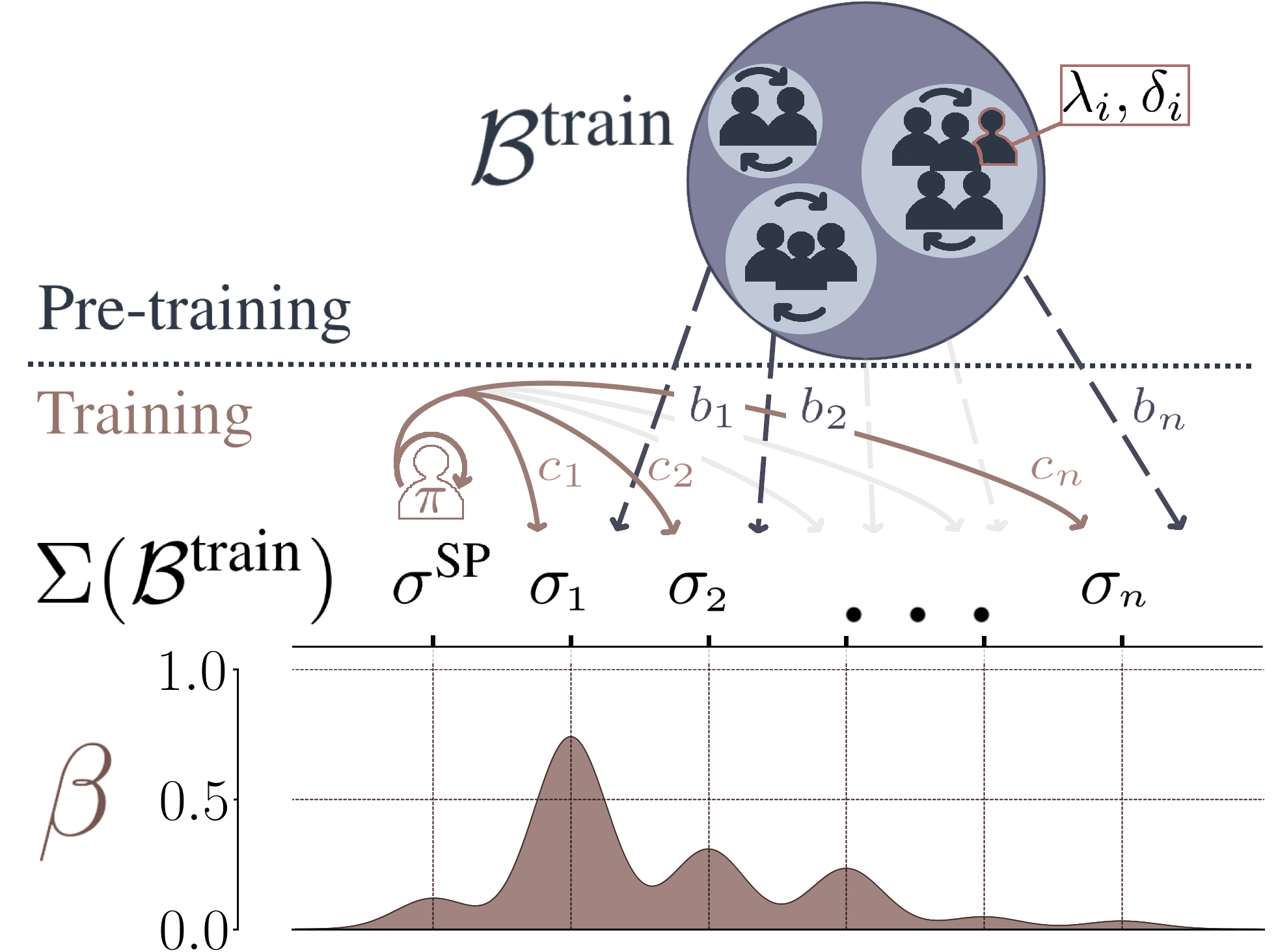
We are interested in learning a robustly cooperative policy $\pi^{f}$ for some $m$-player Partially Observable Markov Game (POMG) $\mu$. \headingScenarios. A scenario $\sigma=(c,\bm{\pi}^{b})$ is characterised by its actors:

  • $c$ focal players $\bm{\pi}^{f}=(\pi^{f},\dots,\pi^{f})$ (all equal to the learned policy).

  • $m-c$ background players $\bm{\pi}^{b}=(\pi^{b}_{1},\dots,\pi^{b}_{m-c})$ (fixed),

  • Each scenario can be seen as its own $c$-player POMG $\mu(\sigma)$.

  • We construct scenario sets with a background population of policies $\mathcal{B}$:

$$\Sigma(\mathcal{B})\coloneqq\{(c,\bm{\pi}^{b})\mid 1\leq c\leq m,\bm{\pi}^{b}\in\mathcal{B}^{m-c}\},$$
\heading

Objectives. We want a policy that reliably maximises utility / minimises regret, regardless of the scenario:

  • $\sigma$-induced reward function $\rho_{\sigma}$; focal actions $\mathbf{a}^{f}=(a^{f}_{1},\dots,a^{f}_{c})$,

    $$\text{{\color\definecolor[named]{pgfstrokecolor}{rgb}{.75,0,.25}{Mean focal utility:}}}\quad U(\pi,\sigma)\coloneqq\sum_{t=1}^{T}\dfrac{1}{c}\sum_{i=1}^{c}\mathbb{E}^{\pi}_{\mu(\sigma)}[\rho_{\sigma}(s_{t},\mathbf{a}^{f}_{t},i)],\hfill$$
  • Maximal utility for scenario $\sigma$, $U^{*}(\sigma)$,

    $$\text{{\color\definecolor[named]{pgfstrokecolor}{rgb}{.75,0,.25}{Regret:}}}\quad R(\pi,\sigma)\coloneqq U^{*}(\sigma)-U(\pi,\sigma).$$

We assess learning methods with the following two-phased protocol: \heading1) Training:

  • A background population of training partners $\mathcal{B}^{\text{train}}$ is provided,

  • A test set of scenarios $\Sigma^{\text{test}}$ is kept held-out,

  • The learner is allowed to do anything for $N$ environment steps.

\heading

2) Testing:

  • No more learning,

  • The obtained policy is evaluated on held-out test scenarios $\Sigma^{\text{test}}$ with: {alertblock}

    Average utility Worst-case utility Worst-case regret
    $\displaystyle U_{\text{avg}}(\pi,\Sigma)=\dfrac{1}{|\Sigma|}\sum_{\sigma\in\Sigma}U(\pi,\sigma),\quad$ $\displaystyle U_{\text{min}}(\pi,\Sigma)=\min_{\sigma\in\Sigma}U(\pi,\sigma),\quad$ $\displaystyle R_{\text{max}}(\pi,\Sigma)=\max_{\sigma\in\Sigma}R(\pi,\sigma).$
{block}

Achieving Robust AHT Two main ingredients:

  • 1)

    Diverse training partners representative of what is in nature.

  • 2)

    An appropriate prior $\beta$ over scenarios.

⇒We pick the minimax prior w.r.t. utility/regret.

With expected utility and Bayesian regret over scenario distributions defined as:

$$U(\pi,\beta)\coloneqq\sum_{\sigma}U(\pi,\sigma)\beta(\sigma),\quad\quad\quad L(\pi,\beta)\coloneqq\sum_{\sigma}R(\pi,\mu)\beta(\sigma).$$
{alertblock}

We play one of the following minimax games:

$$\max_{\pi}\min_{\beta\in\Delta(\Sigma(\mathcal{B}))}U(\pi,\beta),\;\;\text{(1)}\quad\quad\quad\min_{\pi}\max_{\beta\in\Delta(\Sigma(\mathcal{B}))}L(\pi,\beta).\;\;\text{(2)}$$
  • Compute solutions ($\pi^{*},\beta^{*}$) with (stochastic) gradient descent ascent,

  • Convergence guarantees for simple parametrisations of policies,

  • Approximate $c$-player scenarios to single-agent environments by replacing delayed $c-1$ copies with a delayed version of the focal policy $\pi^{f}_{t-d}$.

  • Assumption: No "impossible" scenario.

{column}
{column}
Refer to caption
Figure 1: Training framework proposed in this work.
{block}

Robustness Guarantees Policies $\pi^{*}_{U}$ and $\pi^{*}_{R}$ solving (1) and (2), respectively, have several properties.

In-Distribution: Optimal worst-case utility/regret on the training set.

Out-Of-Distribution: If the true scenarios are all $\epsilon$-close to one of the training scenarios:

$$U_{\text{min}}(\pi^{*}_{U},\Sigma^{\text{true}})>\max_{\pi}\left(U_{\text{min}}(\pi,\Sigma^{\text{train}})-\dfrac{\epsilon T^{2}\lVert\rho\rVert_{\infty}}{2}\right),$$
$$R_{\text{max}}(\pi^{*}_{R},\Sigma^{\text{true}})<\min_{\pi}\left(R_{\text{max}}(\pi,\Sigma^{\text{train}})+\epsilon T^{2}\lVert\rho\rVert_{\infty}\right).$$
{block}

Experimental Results \headingRepeated Prisoner’s Dilemma. (3 rounds, Fully adaptive policies)

Training partners $\mathcal{B}^{\text{train}}$: 9 ad-hoc policies (pure defect/cooperate, tit-for-tat…)

Test partners $\mathcal{B}^{\text{test}}$: 512 sampled policies $\epsilon$-close to training partners ($\epsilon=0.5$).

Table 1: Scores on the repeated Prisoner’s Dilemma. Note: lower regret is better.
  Σ(train)\Sigma(\mathcal{B}^{\text{train}})   Σ(test)\Sigma(\mathcal{B}^{\text{test}})
  UavgU_{\text{avg}}   UminU_{\text{min}}   RmaxR_{\text{max}}   UavgU_{\text{avg}}   UminU_{\text{min}}   RmaxR_{\text{max}}
  Minimax Utility (MU)   $7.69$   $\mathbf{3.00}$   $9.00$   $\mathbf{8.34}$   $\mathbf{3.00}$   $9.00$
  Maximin Regret (MR)   $8.23$   $2.26$   $\mathbf{3.79}$   $7.96$   $2.78$   $\mathbf{4.35}$
  \hdashlinePopulation Best Response (PBR)   $\mathbf{8.54}$   $2.00$   $4.97$   $8.07$   $2.48$   $5.63$
  Fictitious-Play (FP)   $7.06$   $0.14$   $10.56$   $6.33$   $0.56$   $9.96$
  Self-Play (SP)   $7.25$   $0.47$   $10.19$   $6.49$   $0.86$   $9.65$
  Random   $7.40$   $1.50$   $5.50$   $7.47$   $2.18$   $5.20$
ccccd$\mathbf{1}$dc$0.1$d$\mathbf{0.9}$ $\mathbf{1}$ddcd$\mathbf{1}$dd$\mathbf{1}$ $\mathbf{1}$ $\mathbf{1}$
(a) PBR.
dcccc$0.5$d$0.5$dc$0.5$d$0.5$ $0.5$dcc$0.5$d$0.5$dc$0.5$d$0.5$ $0.5$ddcc$0.5$d$0.5$dd$\mathbf{1}$ $\mathbf{1}$ $\mathbf{1}$
(b) MU.
ccccc$\mathbf{0.7}$d$0.3$dc$\mathbf{0.6}$d$0.4$ $\mathbf{0.8}$dcc$\mathbf{0.6}$d$0.4$dc$0.5$d$0.5$ $0.2$ddcd$\mathbf{1}$dd$\mathbf{1}$ $\mathbf{1}$ $\mathbf{0.7}$dcccc$\mathbf{0.6}$d$0.4$dc$\mathbf{0.7}$d$0.3$ $\mathbf{0.8}$dcc$0.5$d$0.5$dc$\mathbf{0.6}$d$0.4$ $0.2$ddcd$\mathbf{1}$dd$\mathbf{1}$ $\mathbf{1}$ $0.3$
(c) MR.
Figure 2: Obtained Policies. Opponent actions are in red.
\heading

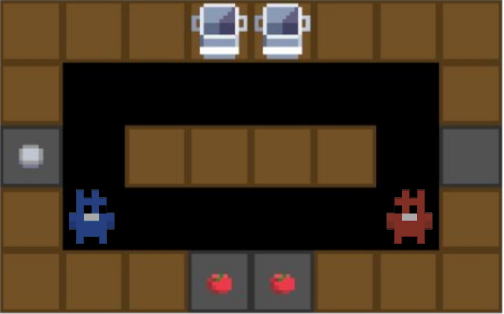
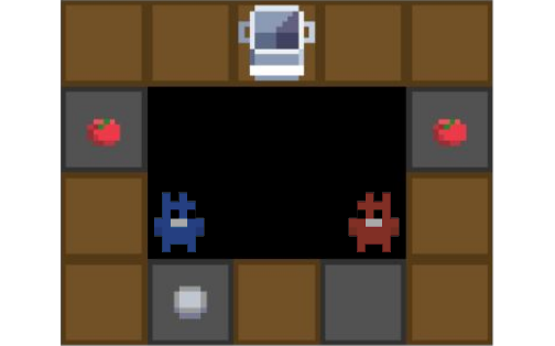
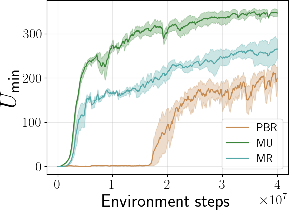
Collaborative Cooking. (Partial observability, LSTM policies)

Training/Test partners: c.f. Figure 1.
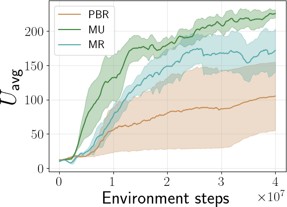
Refer to captionRefer to caption
(a) Circuit layout.
Refer to captionRefer to caption
(b) Circuit layout.
Figure 4: Average utility learning curve over the training scenarios.
Table 2: Scores aggregated over the two kitchen layouts (3 runs).
   Σ(train)\Sigma(\mathcal{B}^{\text{train}})    Σ(test)\Sigma(\mathcal{B}^{\text{test}})
   UavgU_{\text{avg}}    UminU_{\text{min}}    RmaxR_{\text{max}}    UavgU_{\text{avg}}    UminU_{\text{min}}    RmaxR_{\text{max}}
   MU    $\mathbf{266.9{\scriptstyle\pm 4.3}}$    $\mathbf{225.3{\scriptstyle\pm 11.5}}$    $266.0{\scriptstyle\pm 7.9}$    $\mathbf{195.7{\scriptstyle\pm 6.2}}$    $\mathbf{66.0{\scriptstyle\pm 6.8}}$    $266.4{\scriptstyle\pm 10.1}$
   MR    $232.0{\scriptstyle\pm 18.6}$    $144.3{\scriptstyle\pm 14.4}$    $\mathbf{230.7{\scriptstyle\pm 28.2}}$    $172.2{\scriptstyle\pm 15.4}$    $65.1{\scriptstyle\pm 16.0}$    $\mathbf{248.2{\scriptstyle\pm 28.4}}$
   \hdashlinePBR    $209.7{\scriptstyle\pm 23.9}$    $96.8{\scriptstyle\pm 13.4}$    $357.6{\scriptstyle\pm 16.1}$    $151.4{\scriptstyle\pm 19.5}$    $33.6{\scriptstyle\pm 5.9}$    $327.1{\scriptstyle\pm 14.0}$
   FP    $129.9{\scriptstyle\pm 13.9}$    $0.2{\scriptstyle\pm 0.1}$    $483.5{\scriptstyle\pm 16.1}$    $152.2{\scriptstyle\pm 16.8}$    $16.7{\scriptstyle\pm 11.7}$    $369.7{\scriptstyle\pm 19.7}$
   SP    $124.8{\scriptstyle\pm 26.4}$    $15.7{\scriptstyle\pm 10.5}$    $460.8{\scriptstyle\pm 21.7}$    $117.4{\scriptstyle\pm 12.5}$    $6.7{\scriptstyle\pm 3.5}$    $367.5{\scriptstyle\pm 11.6}$
   Random    $42.8{\scriptstyle\pm 0.0}$    $0.0{\scriptstyle\pm 0.0}$    $505.4{\scriptstyle\pm 0.0}$    $32.2{\scriptstyle\pm 0.0}$    $0.0{\scriptstyle\pm 0.0}$    $445.0{\scriptstyle\pm 0.0}$
{column}