Optimal Subspace Inference for the Laplace Approximation of Bayesian Neural Networks

Abstract

Subspace inference for neural networks assumes that a subspace of their parameter space suffices to produce a reliable uncertainty quantification. In this work, we mathematically derive the optimal subspace model to a Bayesian inference scenario based on the Laplace approximation. We demonstrate empirically that, in the optimal case, often a fraction of parameters less than 1% is sufficient to obtain a reliable estimate of the full Laplace approximation. Since the optimal solution is derived, we can evaluate all other subspace models against a baseline. In addition, we give an approximation of our method that is applicable to larger problem settings, in which the optimal solution is not computable, and compare it to existing subspace models from the literature. In general, our approximation scheme outperforms previous work. Furthermore, we present a metric to qualitatively compare different subspace models even if the exact Laplace approximation is unknown.

1 Introduction

Bayesian modelling is an elegant and flexible method to quantify uncertainties of parametric models. Treating the parameters of the model as random variables allows to incorporate model uncertainty. Bayesian neural networks implement this idea for neural networks (NNs) [1, 2, 3, 4, 5]. In practice, however, full posterior inference over Bayesian NNs is intractable due to the large number of parameters that define the NNs. Thus, to quantify the uncertainty of a certain model, practitioners have to approximate the exact posterior distribution by a simpler one. Several methods were developed to make this approximation feasible: The posterior distribution can be approximated, e.g., by variational inference [2, 6, 1, 3, 7, 8]. A different idea, that goes in fact back to the 90s, is to use the technique called Laplace approximation (LA) [9], which has found increasing popularity in recent years due to scalable approximations [10, 11] and its flexible usability [12]. Moreover, in contrast to variational-inference-based approaches, it can be applied to off-the-shelf networks without any retraining: Given a maximum a posteriori (MAP) solution, that often coincides with the minimum of canonical loss functions, the LA replaces the exact posterior by a Gaussian distribution with the MAP as the mean and the inverse of the negative Hessian of the log posterior at the MAP as covariance matrix.

However, this approximation is still infeasible for NNs since the Hessian scales quadratically in the number of parameters such that often it cannot be computed or even stored, let alone be inverted. In addition, training NNs is a high dimensional non-convex optimization problem. In practice fully trained NNs are not located in a minimum of the loss function but rather on a saddle point [13]. Hence, the so-computed Hessian is in general not positive semi-definite [14, 15]. A partial solution to these issues is provided by approximating the Hessian by the generalized Gauss-Newton (GGN) matrix, which is identical to the Fisher Information matrix for common likelihoods [16, 17, 18]. The GGN matrix is positive semi-definite and is constructed from objects that are feasible to compute, cf. Section 3 for details.

However, it’s sheer size makes the GGN matrix still unstorable, even for medium sized networks. Thus, to make the LA feasible for NNs, additional steps are necessary to reduce the size of the Hessian and to allow for an easier computation of its inverse. Common approaches include approximations via a diagonal [10, 19, 20], last layer [21] or a Kronecker-factored [11] structure.

A recent series of works argues that it might suffice to consider partially stochastic NNs [21, 22, 23, 24, 25] that is NNs where the Bayesian inference is performed in a lower dimensional subspace. NNs are heavily overparametrized and the idea is that a subset or well-selected linear combination of parameters is sufficient to obtain reliable uncertainty estimates. We refer to this idea in this work as subspace inference. In [24] this idea is applied to make the LA for Bayesian NNs feasible by storing only a submatrix of the full GGN matrix. The submatrix is constructed using a subset of parameters that can be found via a diagonal approximation of the Hessian [24], via the magnitude of the parameters [26] or via an application of SWAG [5].

The aim of our work is to give a systematic, generic and statistically sound approach to study the usability of subspace inference for the LA of Bayesian NNs. Similar as in [24] we use the widespread [27, 28, 29, 30] combination of the LA with a linearization of our NN $f_{\theta}$ around the MAP value $\hat{\theta}$ of the parameters $\theta$:

$$f_{\mathrm{Lin},\theta}(X)=f_{\hat{\theta}}(X)+J_{X}(\theta-\hat{\theta})\,,$$ (1)

where $J_{X}=\nabla_{\theta}f_{\theta}(X)|_{\theta=\hat{\theta}}$. This method is known as the linearized LA. Our method differs from existing work by making the predictive covariance of the linearized Laplace approximation the centerpiece of our analysis. This viewpoint allows us to give some precise statements of approximation quality and optimality.

The contributions of our article are as follows:

1. We specify a criterion that states when a subspace LA is optimal on a given dataset. We allow for general affine relations, similar to [23], and do not restrict ourselves to a selection of subsets of parameters as in [24].

2. We show that there is an optimal subspace satisfying the criterion from 1 and give a formula for the according affine relation.

3. We demonstrate how this theoretical formula can be used in practice to give a subspace LA and observe that it performs in many cases superior to the subset selection of [24, 12].

4. To measure the performance we propose a new easy-to-compute criterion.

This article is organized as follows: In Section 2 we recall recent work on the subject of the article and then evoke some background on the LA for Bayesian NNs in Section 3. In Section 4 we provide the main theoretical contributions of this work. In Section 5 several experiments to empirically verify our theoretical analysis are carried out. Additional information is provided in the Appendix.

2 Recent Work

Laplace Approximation. The first application of the LA using the Hessian for NNs was introduced by MacKay [9]. [31] also proposed an approximation similar to the generalized Gauss-Newton (GGN) method. The combination of scalable factorizations or diagonal Hessian approximations with the GGN approximation [16, 18] made the LA applicable for larger networks. In particular, the GGN approximation gained more attention due to the introduction of the Kronecker-factored Approximate Curvature (KFAC) [11, 32, 33] which is scalable and outperforms the diagonal Hessian approximation. Due to underfitting issues of the LA [27], the linearized LA based on (1) was developed [28]. We use the same setting in this work.

Partially Stochastic Neural Networks. Studying partially stochastic NNs gained some attention due to their computational efficiency. But even from a statistics viewpoint partially stochastic NNs are attractive because they can capture the uncertainty of the full model by using only a fraction of the parameters. [25] showed that a low-dimensional subspace is sufficient to obtain expressive predictive distributions. They developed the concept of Universal Conditional Distribution Approximators and proved that certain partially stochastic NNs can form samplers of any continuous target conditional distribution arbitrary well. [34] extended this idea to infinitely deep Bayesian NNs.

[23] developed a low-dimensional affine subspace inference scheme. They selected a linear combination of parameter vectors which span a vector space around the MAP. Since this subspace is low-dimensional different methods can be used to approximately sample from the posterior distribution. However, they observed that their uncertainties are too small such that they had to use a tempered posterior to obtain reasonable uncertainties. [24] chose a subset of parameters to construct a subspace model. This subset is selected by the parameters that have the highest posterior variance. However, this work requires quite a large number of parameters to be selected (up to $4\cdot 10^{4}$). Our framework is closest to this work. In contrast, we study the predictive instead of the posterior distribution to obtain a feasible parameter subspace. In addition, we show in the following that neither an ad hoc tempering of the posterior distribution nor thousands of parameters are needed to estimate the uncertainty reliable.

3 Terminology and Background

Setup and Notational Remarks. We consider the supervised learning framework. We model the relation between the independent observable $x$ and the target $y$ by a parametric distribution $p(y|x,\theta)$ with parameters $\theta\in\mathbb{R}^{p}$. Different observations are, as usual, assumed to be independent and identically distributed. We denote the training set of observations as $\mathcal{D}=\{(x_{i},y_{i})|1\leq i\leq N\}$ where $N$ denotes the number of observations. We study regression and classification tasks. $C$ represents the number of outputs $f_{\theta}(x)=(f_{\theta}^{1}(x),\ldots,f_{\theta}^{C}(x))^{\intercal}\in\mathbb{R}^{C}$ of the NN $f_{\theta}$, for both, regression and classification problems. For regression we make a Gaussian model assumption $p(y|x,\theta)=\mathcal{N}(y|f_{\theta}(x),\sigma^{2}\mathbb{1}_{C})$, where only the mean is modelled by the NN. Classification tasks with $C$ classes are modelled by a categorical distribution $p(y|x,\theta)=\mathrm{Cat}\left(y|\phi(f_{\theta}(x))\right)$ with probability vector $\phi(f_{\theta}(x))$, where $\phi$ denotes the softmax function.

We will often consider not a single input sample to $f_{\theta}$ but a whole set such as $X=(x_{1},\ldots,x_{n})$. In this case $f_{\theta}(X)=(f_{\theta}(x_{1})^{\intercal},\ldots,f_{\theta}(x_{n})^{\intercal})^{\intercal}\in\mathbb{R}^{nC}$ should be read as the concatenation of the outputs. We will frequently use the Jacobian of $f_{\theta}$ w.r.t. its parameter $\theta\in\mathbb{R}^{p}$ evaluated at the MAP $\hat{\theta}$ defined in (3) below. Given a set $X$ we concatenate the single input Jacobians along the output dimension and use the symbol

$$J_{X}:=(\nabla_{\theta}f_{\theta}(x_{1})^{\intercal},\ldots,\nabla_{\theta}f_{\theta}(x_{n})^{\intercal})^{\intercal}|_{\theta=\hat{\theta}}\in\mathbb{R}^{nC\times p}\,.$$ (2)

Bayesian Neural Networks. When taking a Bayesian view on NNs the parameter $\theta$ is considered as a random variable equipped with a prior distribution $p(\theta)$. Given the training data $\mathcal{D}=\{(x_{i},y_{i})|1\leq i\leq N\}$, the posterior distribution of $\theta$ is given by $p(\theta|\mathcal{D})\propto p(\theta)p(D|\theta)=p(\theta)\prod_{i=1}^{N}p(y_{i}|x_{i},\theta)$ (with $p(y_{i}|x_{i},\theta)$ as above). A point estimate for $\theta$ is then given by the value that is most likely under $p(\theta|\mathcal{D})$, the so-called MAP (maximum a posteriori) estimate, that is

$$\hat{\theta}=\operatorname*{arg\,min}_{\theta}\mathcal{L}_{\theta}(\mathcal{D})\,,$$ (3)

where we used the (unnormalized) negative log-posterior

$$\mathcal{L}_{\theta}(\mathcal{D})=-\sum_{i=1}^{N}\ln p(y_{i}|x_{i},\theta)-\ln p(\theta)\,.$$ (4)

In this work we will use the common choice $p(\theta)=\mathcal{N}(\theta|0,\lambda^{-1}\mathbb{1}_{p})$ with precision $\lambda>0$ for which (4) just boils down to the MSE loss (for regression) or cross-entropy loss (for classification) combined with L2 regularization.

Laplace Approximation. With $\mathcal{L}_{\theta}(\mathcal{D})$ as in (4) the posterior distribution $p(\theta|\mathcal{D})$ reads as

$$p(\theta|\mathcal{D})=\frac{1}{Z}p(\mathcal{D}|\theta)p(\theta)=\frac{1}{Z}e^{-\mathcal{L}_{\theta}(\mathcal{D})}$$ (5)

with the normalization constant $Z=\int d\theta\;p(\mathcal{D}|\theta)p(\theta)$. For complex models such as Bayesian NNs the exact posterior is typically infeasible to compute or sample from. Expanding (4) to second order around the MAP $\hat{\theta}$ from (3), we obtain

$$\mathcal{L}_{\theta}(\mathcal{D})\simeq\mathcal{L}_{\hat{\theta}}(\mathcal{D})+\frac{1}{2}\left(\theta-\hat{\theta}\right)^{\intercal}\left(\nabla_{\theta}^{2}\mathcal{L}_{\theta}(\mathcal{D})|_{\theta=\hat{\theta}}\right)\left(\theta-\hat{\theta}\right)\,.$$

Inserting this expansion in (5) we arrive at the Laplace approximation of the posterior

$$p(\theta|\mathcal{D})\simeq\mathcal{N}(\theta|\hat{\theta},\Psi)$$

with mean $\hat{\theta}$ and covariance $\Psi=\left(\nabla_{\theta}^{2}\mathcal{L}_{\theta}(\mathcal{D})|_{\theta=\hat{\theta}}\right)^{-1}=\left(NH+\lambda\mathbb{1}_{p}\right)^{-1}\in\mathbb{R}^{p\times p}$, where we denote by $H=-\frac{1}{N}\sum_{i=1}^{N}\nabla_{\theta}^{2}\ln p(y_{i}|\theta,x_{i})|_{\theta=\hat{\theta}}$ the Hessian of the averaged negative log-likelihood.

Generalized Gauss-Newton Matrix. The Hessian $H\in\mathbb{R}^{p\times p}$ from above is the second order derivative of the averaged negative-log-likelihood $-\frac{1}{N}\ln p(\mathcal{D}|\theta)$ at the MAP $\hat{\theta}$. On the one hand, to compute $H$ is infeasible, and on the other hand, even if $H$ could be computed, it would be impossible to store the $\frac{p\left(p+1\right)}{2}$ free components, since $p\gg 1$. In addition, for trained NNs the Hessian does usually not have the nice property of positive semi-definiteness that is found, e.g., in the context of convex problems, because the learned MAP $\hat{\theta}$ is, in general, not a local minimum but rather a saddle point. These difficulties of computational complexity and missing positive definiteness can be overcome by using the generalized Gauss-Newton (GGN) matrix [16] instead of $H$:

$$H_{\mathrm{GGN}}=\frac{1}{N}\sum_{i=1}^{N}J^{\intercal}_{f_{i}}H_{\text{-}\ln p(y_{i}|f_{i})}J_{f_{i}}\,,$$ (6)

where $J_{f_{i}}=\nabla_{\theta}f_{\theta}(x_{i})|_{\theta=\hat{\theta}}\in\mathbb{R}^{C\times p}$ and $H_{\text{-}\ln p(y_{i}|f_{i})}=-\nabla_{f}^{2}\ln p(y_{i}|f_{i})|_{f_{i}=f_{\hat{\theta}}(x_{i})}\in\mathbb{R}^{C\times C}$ is the Hessian of the negative log-likelihood w.r.t. model output ${f_{i}}=f_{\theta}(x_{i})$. $H_{\mathrm{GGN}}$ can be interpreted as the Hessian of the linearized model [18, 28] and is positive semi-definite if the $H_{\text{-}\ln p(y|f_{i})}$ are positive-semi definite [16], which is the case in our work. More detailed information on $H_{\mathrm{GGN}}$ and the relation between $H_{\mathrm{GGN}}$ and $H$ is provided in Appendix G. Combining (6) with the term arising from the prior $p(\theta)$ we obtain the following precision matrix of the Laplace approximated model

$$\Psi_{\mathrm{GGN}}^{-1}=\sum_{i=1}^{N}J^{\intercal}_{f_{i}}H_{\text{-}\ln p(y_{i}|f_{i})}J_{f_{i}}+\lambda\mathbb{1}_{p}\,.$$ (7)

Approximations. While the GGN relation (6) consists of objects, $J_{f_{i}}$ and $H_{\text{-}\ln p(y_{i}|f_{i})}$, that are scalable in their computation we usually can’t compute $H_{\mathrm{GGN}}$ or $\Psi_{\mathrm{GGN}}^{-1}$ as the resulting matrices have still too many dimensions for modern NNs. In particular, we can’t invert $\Psi_{\mathrm{GGN}}^{-1}$ to obtain the posterior covariance $\Psi_{\mathrm{GGN}}$. As a consequence, various approximations have been developed that modify the structure in such a way that it takes less amount of storage and is easier to invert. An easy solution is to only keep the diagonal of $\Psi_{\mathrm{GGN}}$. In the KFAC approximation the Hessian is reduced to a form where it is the Kronecker product of two smaller matrices.

Equivalence Between GGN and Fisher Information. For the computations in our experiments we use the Fisher information matrix $\mathcal{I}$ instead of $H_{\mathrm{GGN}}$ which are identical objects for the cases considered in this work [35, 18, 13], cf. Appendix G.4. As follows from the identities in Appendix G.1 we have $\mathcal{I}=VV^{\intercal}$ with a $V\in\mathbb{R}^{p\times NC}$ that can be computed via minibatches from $\mathcal{D}$ and expressions that involve first order derivatives of $f_{\theta}$. This allows us to compute for any matrix $P\in\mathbb{R}^{p\times s}$ the expression

$$P^{\intercal}H_{\mathrm{GGN}}P=P^{\intercal}\mathcal{I}P=(VP)^{\intercal}VP\in\mathbb{R}^{s\times s}$$ (8)

in a scalable manner if $s$ is sufficiently small. Thus, while we often can’t actually compute $H_{\mathrm{GGN}}$ or $\mathcal{I}$ in practice, we can usually compute quadratic forms such as (8).

Predictive Distribution. For the posterior distribution $p(\theta|\mathcal{D})$ and a set of $n$ inputs $X$ the posterior predictive distribution is given by

$$p(Y|X,\mathcal{D})=\int d\theta\;p(Y|X,\theta)p(\theta|\mathcal{D}).$$ (9)

Under the LA and using the linearized model (1) for $p(Y|X,\mathcal{D})$ we can give an explicit formula to this distribution for regression problems

$$p(Y|X,\mathcal{D}) \simeq\mathcal{N}(Y|f_{\hat{\theta}}(X),\Sigma_{X}+\sigma^{2}\mathbb{1}_{nC})$$ (10)

$$\text{with}\quad\Sigma_{X} =J_{X}\Psi J_{X}^{\intercal}\in\mathbb{R}^{nC\times nC}$$ (11)

denoting the model uncertainty part of the predictive covariance. For classification tasks the predictive distribution can be approximated by the probit approximation [36]

$$\begin{split}p(Y|X,\mathcal{D})\simeq\mathrm{Cat}\left(Y|\phi\left(\frac{f_{\hat{\theta}}(X)}{\sqrt{1+\frac{\pi}{8}\mathrm{diag}\Sigma_{X}}}\right)\right)\end{split}$$ (12)

with $\Sigma_{X}$ as in (11) and the softmax function $\phi$. Note that in both cases, regression and classification, the predictive distribution is essentially fixed by $\Sigma_{X}$ from (11), which is why this object will be the linchpin of our analysis below. We will call $\Sigma_{X}$ the epistemic predictive covariance.

4 The Laplace Approximation for Subspace Models

Subspace Models. In this work we study, as in [23], models that are defined on an affine subspace of the parameter space $\mathbb{R}^{p}$ chosen to contain the MAP $\hat{\theta}$ from (3). That is, we consider a re-parametrization

$$\theta=\hat{\theta}+P\mu\,,$$ (13)

where $P\in\mathbb{R}^{p\times s}$ is a matrix that we call, somewhat loosely, the projection matrix (in general it’s not related to a mathematical projection) and $\mu$ is a new parameter that runs through $\mathbb{R}^{s}$ where $s\leq p$ is the subspace dimension. The assumption in considering Bayesian inference of NNs in a subspace is that only a fraction of the parameter space is actually needed to represent the (epistemic) uncertainty faithfully.

Note that the selection of a subset of parameters on which to perform inference, as it’s done in [24, 25], is a special case of (13), as can be seen by choosing $P=(e_{i_{1}},\ldots,e_{i_{s}})$ as a concatenation of canonical basis vectors, where the set $\{i_{j}|1\leq j\leq s\}\subseteq\{1,\ldots,p\}$ corresponds to the chosen subset.

Bayesian Inference for $\mu$. To perform Bayesian inference in the subspace model, we choose the following prior

$$\tilde{p}(\mu)=\mathcal{N}(\mu|0,\left(\lambda P^{\intercal}P\right)^{-1})\,,$$ (14)

where $\mu$ is the random variable in this subspace and we recall that $\lambda$ is the precision of $p(\theta)$. The set of maps $P$ that we analyse in this work can always be chosen such that $P^{\intercal}P=\mathbb{1}_{s}$. Together with the following likelihood

$$\tilde{p}(\mathcal{D}|\mu)=p(\mathcal{D}|\hat{\theta}+P\mu)$$ (15)

that is induced by (13), the following lemma holds:

Lemma 1.

In the setting above, consider a full rank $P\in\mathbb{R}^{p\times s}$. For the posterior $\tilde{p}(\mu|\mathcal{D})\propto\tilde{p}(\mu)\tilde{p}(\mathcal{D}|\mu)$ with prior $\tilde{p}(\mu)$ as in (14) we have the LA

$$\tilde{p}(\mu|\mathcal{D})\simeq\mathcal{N}(0,(P^{\intercal}\Psi^{-1}P)^{-1})\,.$$ (16)

Lemma 1 is true because from (15) and (14), we can deduce $-\nabla_{\mu}^{2}\ln\left(\tilde{p}(\mathcal{D}|\mu)\tilde{p}(\mu)\right)|_{\mu=0}=P^{\intercal}(NH+\lambda\mathbb{1}_{p})P=P^{\intercal}\Psi^{-1}P$.

We will find in Theorem 1 below that the family of posteriors (16) is rich enough to approximate the full LA optimally in a certain sense when a suitable $P$ is chosen.

Predictive Distributions of Subspace Models. Similar to (1) we linearize $\tilde{f}_{\mu}=f_{\hat{\theta}+P\mu}$ around $\mu=0$ to obtain for a set of $n$ inputs $X$

$$\tilde{f}_{\mathrm{Lin},\mu}(X)=f_{\hat{\theta}}(X)+J_{X}P(\mu-0)\,,$$ (17)

where we denoted, as in (1), by $J_{X}=\nabla_{\theta}f_{\theta}(X)|_{\theta=\hat{\theta}}\in\mathbb{R}^{nC\times p}$ the Jacobian of the full network at the MAP.

Combining (16) with (17) we obtain as above the predictive distributions

$$\begin{gathered}\mathcal{N}(Y|f_{\hat{\theta}}(X),\Sigma_{P,X}+\sigma^{2}\mathbb{1}_{nC}),\\ \mathrm{Cat}\left(Y|\phi\left(\frac{f_{\hat{\theta}}(X)}{\sqrt{1+\frac{\pi}{8}\mathrm{diag}\Sigma_{P,X}}}\right)\right),\end{gathered}$$ (18)

for the LAs of a subspace model with the notation

$$\Sigma_{P,X}=J_{X}P(P^{\intercal}\Psi^{-1}P)^{-1}P^{\intercal}J_{X}^{\intercal}\in\mathbb{R}^{nC\times nC}$$ (19)

for its epistemic predictive covariance.

Evaluation of $P$. We would like to find a subspace model (13) whose LA closely aligns with the (typically infeasible) LA of the full model. The subspace model is fixed by the projection matrix $P$. As the posterior predictive distribution (9) is the object of genuine interest for prediction via Bayesian NNs it is natural to require that the distributions in (10), (12) and in (18) are as similar as possible. As those distributions arise from each other by replacing the epistemic predictive covariance, i.e. replacing $\Sigma_{X}$ by $\Sigma_{P,X}$, we can measure the approximation quality by the relative error

$$\frac{\lVert\Sigma_{X}-\Sigma_{P,X}\rVert_{F}}{\lVert\Sigma_{X}\rVert_{F}}\,,$$ (20)

where we use the Frobenius norm $\lVert\ldots\rVert_{F}$.

4.1 The Optimal Subspace Model

Consider a set of $n$ inputs $X=\left(x_{1},\ldots,x_{n}\right)$. This could be the set of inputs in the training set $\mathcal{D}$ or a subset of the latter. Given this set $X$ and a fixed subspace dimension $s\leq p$ we want to find the optimal $P^{*}\in\mathbb{R}^{p\times s}$ that solves the following minimization problem

$$P^{*}\in\operatorname*{arg\,min}_{P\in\mathbb{R}^{p\times s},\,\mathrm{rank}\,P=s}\|\Sigma_{P,X}-\Sigma_{X}\|_{F}\,,$$ (21)

where the epistemic predictive covariances are defined as in (11) and (19). A solution to this problem will then also minimize the relative error (20). Note that such a solution is never unique. In fact, for any $P^{*}$ that solves (21) we can also consider $P^{*}Q$ for an arbitrary invertible $Q\in\mathbb{R}^{s\times s}$ since we have $\Sigma_{P^{*}Q,X}=\Sigma_{P^{*},X}$, cf. (19).

For the solution of the problem (21) we will need the eigenvalue decomposition $\Sigma_{X}=J_{X}\Psi J_{X}=U\Lambda U^{\intercal}$ where $U$ is an orthogonal matrix and $\Lambda\in\mathbb{R}^{nC\times nC}$ is a positive semi-definite diagonal matrix. We choose this eigendecomposition such that the diagonal entries of $\Lambda$ are decreasing. We will use the Eckart-Young-Mirsky-Theorem [37, 38, 39] which states that the following low rank problem has an explicit solution

$$U_{s}\Lambda_{s}U_{s}^{\intercal}\in\operatorname*{arg\,min}_{A\in\mathbb{R}^{nC\times nC}:\,\mathrm{rank}\,A\leq s}\|A-\Sigma_{X}\|_{F}\,,$$ (22)

where $U_{s}\in\mathbb{R}^{nC\times s}$ contains the first $s$ eigenvectors, called dominant eigenvectors from now on, and $\Lambda_{s}\in\mathbb{R}^{s\times s}$ is the reduced diagonal matrix obtained by taking the upper $s\times s$ block containing the $s$ leading eigenvalues of $\Sigma_{X}$. The following theorem shows that the LA to a subspace model can reach the rank-$s$ minimum from (22) for a suitable class of $P^{*}$.

Theorem 1 (Existence of an optimal subspace model for the Laplace approximation).

Consider the problem (21) with $s\leq s_{\mathrm{max}}=\min(nC,p)$. Suppose that $J_{X}\in\mathbb{R}^{nC\times p}$ has full rank. For any invertible $Q\in\mathbb{R}^{s\times s}$ the matrix

$$P^{*}=\Psi J_{X}^{\intercal}U_{s}Q$$ (23)

solves (21). For any such $P^{*}$ we have

$$\Sigma_{P^{*},X}=U_{s}\Lambda_{s}U_{s}^{\intercal}.$$ (24)

The proof is provided in Appendix B. The restriction to dimensions below $s_{\mathrm{max}}=\min(nC,p)$ and the assumption on the full rank of $J_{X}$ is needed to assure that $P^{*}$ has full rank which is required for $\Sigma_{P^{*},X}$ in order to be well-defined. If $J_{X}$ doesn’t have full rank, we restrict the experiments to the rank of the Jacobian. This is done in some regression problems in Section 5.

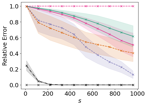
(a) ENB

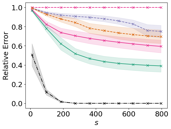
(b) Red Wine

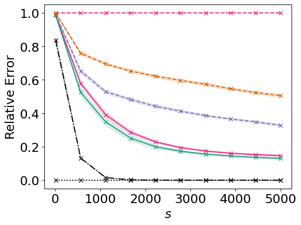
(c) California

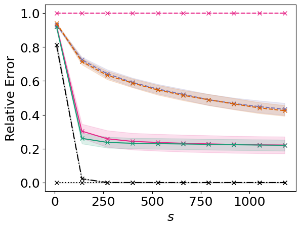
(d) Naval Propulsion

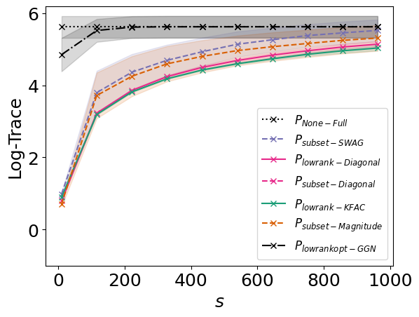
(e) ENB

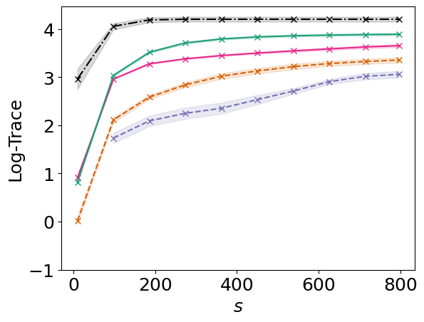
(f) Red Wine

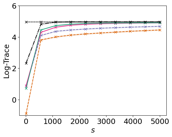
(g) California

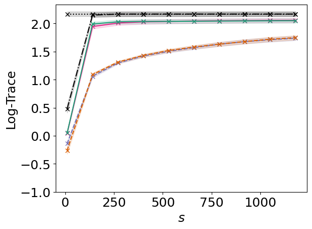
(h) Naval Propulsion

Figure 1: Comparison of low rank approximations and subset methods for different regression datasets. Different choices of $P$ are marked by different colours and line types. The first row displays the relative error (20) and the second the logarithm of the trace (25) of the epistemic covariance matrix. Missing values in the logarithm of trace plots have a trace of zero at these values of $s$ (e.g. SWAG for the lowest $s$ in Red Wine.)

4.2 Applying Theorem 1 in Practice

Theorem 1 states that there is an optimal solution to problem (21) and it is, to the best knowledge of the authors, the first systematic solution to a subspace modelling for Bayesian NNs in the context of LA. However, applying Theorem 1 in practice will usually not be possible, due to the following reasons:

Epistemic Limitation. Training datasets $\mathcal{D}$ are often so large that computing a eigendecomposition of $\Sigma_{X}$ and thus of $U_{s}$ is infeasible. However, even if we can pick $X=\mathcal{D}$ we actually want the subspace model to work for unseen data points, that is data points that are not contained in $\mathcal{D}$.

No Access to $\Psi$. The posterior covariance $\Psi$ from the LA is usually not available. In fact, if it was, this would raise the question of why to use a subspace model at all.

In practice we will therefore use the following workflow:

1. Fix an approximation $\Psi_{\mathrm{approx}}$ to $\Psi$ such as the KFAC or diagonal approximation.

2. Use a subset $X^{\prime}$ of size $n$ of the inputs in the training set to construct $J_{X^{\prime}}\Psi_{\mathrm{approx}}J_{X^{\prime}}^{\intercal}\in\mathbb{R}^{nC\times nC}$ and determine its $s$ dominant eigenvectors $U_{s}\in\mathbb{R}^{nC\times s}$

3. Construct $P$ via $P=\Psi_{\mathrm{approx}}J_{X^{\prime}}^{\intercal}U_{s}$ (we will in this work $Q$ fix to be always the identity).

4. For the $X$ of interest (usually not contained in the training set), compute the predictive covariance $J_{X}P(P^{\intercal}\Psi P)^{-1}P^{\intercal}J_{X}^{\intercal}$. Note, that we can really use the GGN $\Psi$ here, since $\Psi_{\mathrm{GGN}}=VV^{\intercal}$ can be written as an outer product which allows for a batch-wise computation, cf. (8). For our experiments we used an $X$ of size $n$ that was randomly drawn from the test data.

As our construct deviates due to $X^{\prime}\neq X$ and $\Psi_{\mathrm{approx}}\neq\Psi$ from the setting in Theorem 1 we do not have any longer a guarantee of choosing an optimal $P$. In Section 5 we study therefore empirically the performance of the above construction on various datasets.

Trace Metric for $P$. The relative error (20) quantifies the deviation of the subspace model to the full LA. As the latter is usually not known we propose a different metric that gives qualitatively the same ranking of the subspace models as we empirically demonstrate in Section 5. Heuristically, $\Sigma_{P,X}$ approximates better $\Sigma_{X}$ if it contains the dominant eigenspace, because in the directions of these eigenvectors the covariance has its largest contributions. Hence, we propose as an alternative to (20) the trace criterion: If

$$0\leq\operatorname{Tr}\Sigma_{P_{1},X}<\operatorname{Tr}\Sigma_{P_{2},X}\leq\operatorname{Tr}\Sigma_{X}$$ (25)

holds, $P_{2}$ is a better projector than $P_{1}$. A larger trace value indicates that the more dominant eigenspace is captured for a given $P$. The proof of $\operatorname{Tr}\Sigma_{P,X}\leq\operatorname{Tr}\Sigma_{X}$ and an extended explanation are given in Appendix C.

5 Experiments

For our experiments we use various regression datasets from OpenML [40] [41] as well as common classification tasks as MNIST [42], a corrupted version of MNIST [43], FashionMNIST [44], CIFAR10 [45] and a subset of ImageNet [46], called ImageNet10, that contains only the ten classes listed in Appendix A. Details about the used NNs can be found in Appendix A and the repository. We compare the following LAs:

• $P_{\mathrm{subset-Magnitude}},P_{\mathrm{subset-Diagonal}}$ and $P_{\mathrm{subset-SWAG}}$ (dashed lines) select a subset of parameters according to the magnitude of parameters, the diagonal GGN approximation or variances produced via SWAG. We use the term subset methods for these approximations from [24, 12] because they select certain parameters to construct $P$.

• $P_{\mathrm{lowrank-KFAC}}$ and $P_{\mathrm{lowrank-Diagonal}}$ (solid lines) are constructed as in Section 4.2 and use a KFAC or a diagonal GGN approximation to estimate $\Psi$. Hence, these construction are based on an approximation of the posterior covariance $\Psi$ (cf. Section 4.2). We use the term low rank methods for these since Theorem 1 bases its argument on a low rank approximation. A subset of the training data was used for the construction of these subspace models, cf. Appendix A.3.

• Moreover, where feasible, we show results for a $P_{\mathrm{lowrankopt-GGN}}$ (dashed-dotted line) that is exactly constructed as in Theorem 1 by using the test data and the $\Psi_{\mathrm{GGN}}$ for the construction of the subspace model. This is the optimal subspace model for a given $s$. $P_{\mathrm{None-Full}}$ (dotted line) is the regular LA without any dimensional reduction.

All experiments are done with five different seeds and the average of the results is plotted with markers. To enhance the visualization, the markers are linearly interpolated by lines whose type indicates the methods used to approximate the LA. The shaded area around the mean value illustrates the sample standard error. All plots use the same colour and line coding.

To evaluate the different subspace models (13), parametrized by $P\in\mathbb{R}^{p\times s}$, we use the relative error (20) because it quantifies the approximation quality of the epistemic predictive covariance $\Sigma_{P,X}$ w.r.t. the full epistemic predictive covariance matrix $\Sigma_{X}$. In addition, we use the auxiliary trace metric (25) to empirically verify that it yields qualitatively the same ordering as the relative error. This enables us to compare subspace models if the relative error isn’t computable. In addition, we also studied the widespread NLL metric, which however yielded inconsistent results for the problem studied in this work. The results and an according discussion are provided in Appendix F.

Regression Datasets. Figure 1 shows the relative error (20) and the logarithm of the trace criterion (25) (log-trace) for different regression datasets and the subspace models listed above for different $s$. For ENB, Red Wine and Naval Propulsion the Jacobian is rank-deficient, so that only $s$ up to the rank of the Jacobian on the training data are considered. California is plotted up to $s=5000$. First, we observe that the ideal subspace model (black dashed-dotted line) needs only a fraction of the number of model parameters that are around 18000 to reach a small relative error. The exact number of parameters is listed in Table 4 in the Appendix A. Hence, subspace models can be suitable to quantify the uncertainty provided by a LA. However, $P_{\mathrm{lowrankopt-GGN}}$ is usually unknown such that the ideal approximation isn’t available. Comparing the feasible approximations in Figure 1 we find that low rank approximations demonstrate superior approximations compared to subset methods in general. In particular, the performance of $P_{\mathrm{subset-Diagonal}}$ is strictly inferior to $P_{\mathrm{lowrank-Diagonal}}$. For ENB the subset methods obtain a better performance. We speculate that the different performance on this dataset is related to the number of ‘dead parameters’ whose gradient is almost zero, which provides a natural subset to be selected. Indeed, ENB has the most number of dead parameters with 93%. More details on this investigation are given in Appendix E.

A comparison between the first and the second row of Figure 1 demonstrates that the log-trace retains the ordering of the relative error. Differences are rare and if they happen they are small and usually contained in the sample standard deviation.

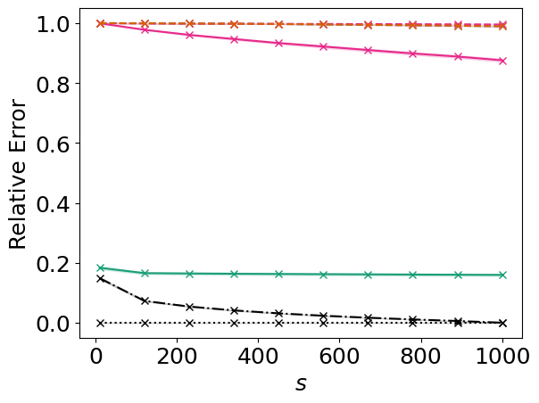
(a) MNIST

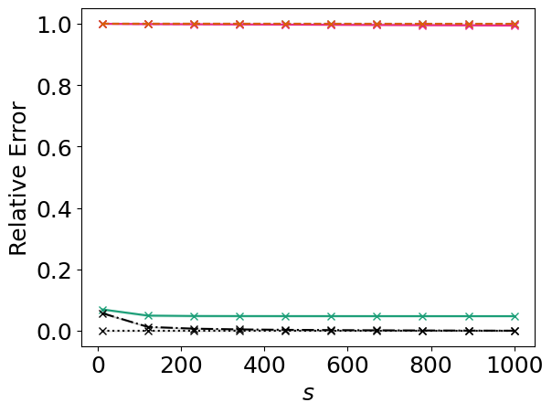
(b) FashionMNIST

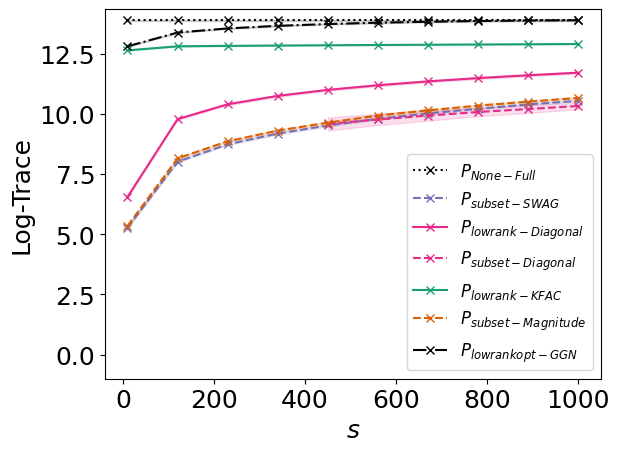
(c) MNIST

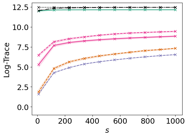
(d) FashionMNIST

Figure 2: Relative error (20) and logarithm of trace (25) of the epistemic covariance matrix for MNIST and FashionMNIST.

Classification Tasks. MNIST and FashionMNIST are trained with small CNNs such that the relative error is computable. For these datasets the discrepancy between low rank and subset methods is even larger. Figure 2 shows that the subset methods yield a relative error of approximately 1.0 which implies that these methods aren’t able to approximate the full covariance matrix. Only for very large $s$ the relative error starts to decrease which demonstrates that these methods fail to approximate the full solution effectively (cf. Appendix D). $P_{\mathrm{lowrank-KFAC}}$ shows the best performance. It’s relative error decreases below $0.2$ and $0.1$ for $s=10$ for MNIST and FashionMNIST, respectively, and the large trace values indicate that $P_{\mathrm{lowrank-KFAC}}$ parametrizes the eigenspace corresponding to the largest eigenvalues of $\Sigma_{X}$, well.

In Figure 3 the quality of the approximation on out-of-distribution data is evaluated. We use the NNs that were trained on MNIST but apply them on corrupted test data. 15 different corruptions are studied. For each subspace dimension we consider, as above, various choices of $P$ indicated by different colours, where the same coding as in Figures 1 and 2 applies. The relative error and the trace of different subspace models for $s\in\{100,500,1000\}$ are plotted in Figure 3. While the optimal low rank approximation yields good results, the performance of all the other methods decreases. E.g. for certain corruptions like brightness and fog all non-optimal subspace models perform bad. These results indicate that the performance on the subspace models depends on the nature of the out-of distribution data. Interestingly, we can observe that the jump from $s=100$ to $s=1000$ has far less impact on the relative error of subset methods than the transition to a $P$ as constructed in Section 4.2. Hence, the approximation method is more important than the size $s$ of the subspace.

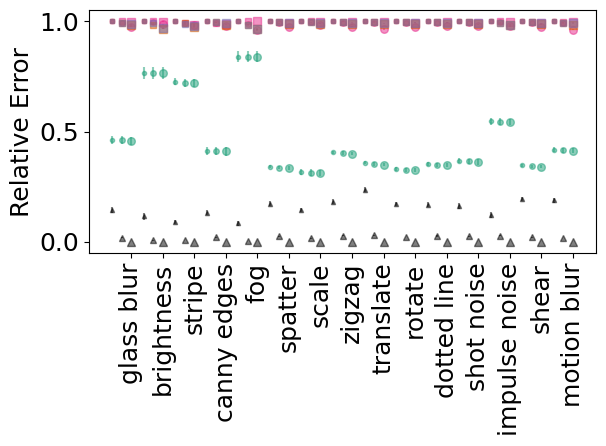
(a) Relative error

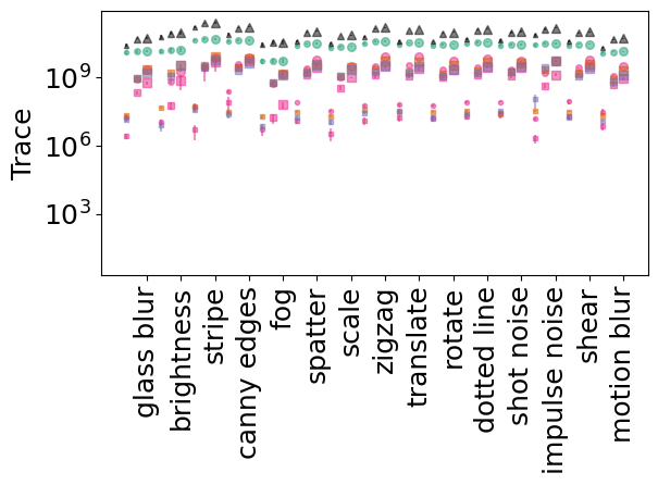
(b) Trace criterion

Figure 3: Relative error (20) (left) and trace criterion (25) (right) for corrupted MNIST datasets [43] and three different dimensions $s=100,\,500,\,1000$ (shown by markers in increasing size). Different choices for $P$ are indicated by different colours and marker shapes: Square markers $\blacksquare$ indicate subset based methods, whereas discs $\bullet$ indicate low-rank based methods (proposed in this work). The colour coding is chosen as in Figure 1. Note there are two $P$s constructed from a diagonal approximation to the Hessian that either use a subset (pink squares) or a low rank based (pink circles) approach. Results were obtained by averaging over five seeds. Standard errors are depicted by bars, where the latter are larger than the marker size.

In Figure 4 we consider a ResNet9 for CIFAR10 and a ResNet18 for ImageNet10. For computational reasons we restricted our analysis for ImageNet10 to $s\leq 30$. For both networks the number of parameters is so large that $\Sigma_{X}$ and thus the relative error is computationally infeasible. While the relative error is not available we can, however, still evaluate different methods with the trace criterion (25). Figure 4 confirms our observations from lower dimensional problems. $P_{\mathrm{lowrank-KFAC}}$ is superior to all other methods and the low dimensional eigenspace of $\Sigma_{X}$ spanned by the selected eigenvectors in parameter space is orders of magnitude higher for $P_{\mathrm{lowrank-KFAC}}$ in CIFAR10 compared to all other methods. In ImageNet10 both low rank approximations perform well, but the subspace methods fail.

In all of our classification experiments the performance of the subset methods is quite unsatisfying. The only acceptable approximation is obtained by $P_{\mathrm{lowrank-KFAC}}$. This trend is also reflected in the traces of the epistemic covariance matrices. Hence, none of the methods but $P_{\mathrm{lowrank-KFAC}}$ is able to select the eigenvector corresponding to the largest eigenvalues in parameter space and so to approximate $\Sigma_{P,X}$ well.

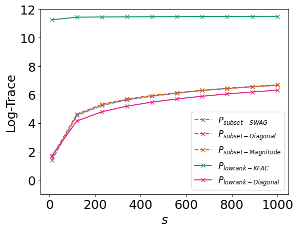
(a) CIFAR10

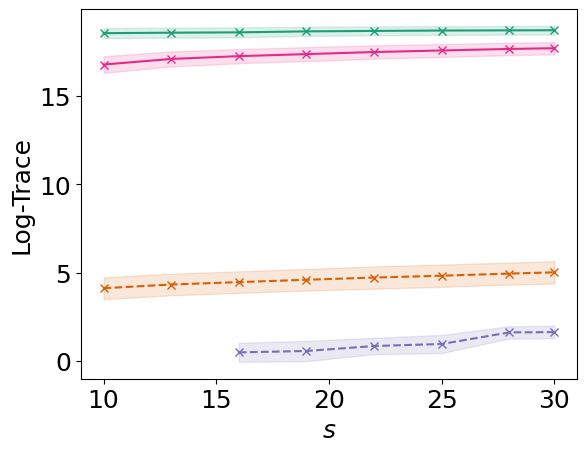
(b) ImageNet10

Figure 4: Evaluation with the trace criterion (25) for CIFAR10 and ImageNet10 and different choices of $P$. Missing values in Figure 4(b) are due to vanishing trace values.

6 Conclusion

In this work we propose to look at subspace Laplace approximations of Bayesian neural networks through the lens of their predictive covariances. This approach allows us to derive the existence of an optimal subspace model via low rank techniques and yields a natural metric, the relative error, to judge the approximation quality. To make these theoretical insights practically usable we propose a subspace model that is conceptually based on the optimal solution and provide a metric that we observe empirically to correlate well with the relative error. The proposed subspace model outperforms existing methods on the studied datasets. In fact, we observe that a well chosen method for subspace construction can often have more impact than an increase in the subspace dimension $s$. In practice our proposed subspace model has to rely on approximations of the posterior covariance. Our experiments demonstrate that the quality of our method depends strongly on these as the different performance of $P_{\mathrm{lowrank-KFAC}}$ and $P_{\mathrm{lowrank-Diagonal}}$ illustrates. A further restriction of our low rank based approach is its computational dependency on the number of model parameters $p$ because the projection $P\in\mathbb{R}^{p\times s}$ has to be explicitly stored.

Even though the optimality of the projector $P_{\mathrm{lowrankopt-GGN}}$ is proven, it isn’t clear that this solution is unique. If there was another optimal solution that is computationally more feasible the practicability could be improved.

Appendix A Experiments

A.1 Architectures and Training

The code of all experiments was developed in PyTorch [47].

The regression datasets are obtained by OpenML [40, 41] and the expected mean $E_{y\sim p(y|x,\theta)}[y]$ is estimated by multi-layer perceptrons (MLPs) with ReLU activation functions and two hidden layers that include 128 units in each layer. The bias term is used as well. A full batch training is performed in each epoch, i.e. the batch size equals the size of the training set. The input data is normalized with respect to its mean value and its standard deviation. Further details of the architecture and training procedure are given in Table 1.

dataset	$\alpha_{\text{init}}$	$n_{\mathrm{epoch}}$	warm up/ decay
Red Wine	$0.0004$	300	(0.3/0.3)
ENB	$0.004$	1500	(0.1/0.5)
California	$0.0004$	100	(0.3/0.5)
Naval Propulsion	$0.0004$	100	(0.3/0.5)

Table 1: The architecture of all networks trained on regression datasets is an MLP with two hidden layers with 128 neurons each. After each hidden layer a ReLU is used. The models are trained on $n_{\mathrm{epoch}}$ epochs with learning rate $\alpha=\alpha_{\text{init}}\frac{b}{256}$ ($b$ is the batch size which here equals the number of training data points). For the fraction of epochs ‘warm up’ the learning rate is linearly increased to $\alpha$ and starting from the fraction of epochs ‘decay’ the learning rate is linearly decreased.

The architecture of MNIST [42] and FashionMNIST [44] is a small hand-designed convolutional network (CNN) with 2d-convolutions, max-pooling, batch normalization and ReLU activation function. Before the softmax function a linear layer is applied. The exact architecture can be found in the linked code. To train the CNNs, the input data is mapped to the interval $\left[0,1\right]$ and then normalized with “mean” and “standard deviation” $0.5$. Additional details are given in Table 2.

dataset	$\alpha$	$n_{\mathrm{epoch}}$	warm up/ decay
MNIST	$0.004$	20	(0.1/0.3)
FashionMNIST	$0.002$	40	(0.1/0.5)

Table 2: The models are trained on $n_{\mathrm{epoch}}$ epochs with learning rate $\alpha$ and batch size $b=256$. For the fraction of epochs ‘warm up’ the learning rate is linearely increased to $\alpha$ and starting from the fraction of epochs ‘decay’ the learning rate is linearly decreased.

CIFAR10 [45] and ImageNet10 [46] are classified by ResNet architectures [48]. CIFAR10 is trained from scratch with ResNet9, but for ImageNet10 the pretrained ResNet18 from Pytorch with weights IMAGENET1K_V1 is chosen, where the last layer is replaced by a linear layer with 10 classes. During training the images are normalized with respect to their channelwise pixel mean and pixel standard deviation. In addition random flips are applied on both datasets. For CIFAR10 greyscale and random crops are used, too. More information is provided in Table 3.

dataset	$\alpha$	$n_{\mathrm{epoch}}$	warm up/ decay
CIFAR10	$\ 0.004$	100	(0.1/0.7)
ImageNet10	0.0004	10	(0.5/0.5)

Table 3: The models are trained on $n_{\mathrm{epoch}}$ epochs with learning rate $\alpha$ and batch size $b=256$. For the fraction of epochs ‘warm up’ the learning rate is linearly increased to $\alpha$ and starting from the fraction of epochs ‘decay’ the learning rate is linearly decreased.

To evaluate the quality of the dimensional reduction, the size of the different models that are used for predictions are required. Table 4 lists the number of model parameters. The number of model parameters of the MLP and CNN has been chosen large enough such that the prediction performance is satisfying, but is also limited to be able to compute $P_{\mathrm{lowrankopt-GGN}}$.

dataset	model	$p$
California	MLP	17,793
ENB	MLP	17,922
Naval	MLP	18,690
Red Wine	MLP	18,177
MNIST	CNN	12,458
FashionMNIST	CNN	12,458
CIFAR10	ResNet9	668,234
ImageNet10	ResNet18	11,181,642

Table 4: Number of trainable parameters $p$ for each model that is trained on the corresponding dataset.

A.2 ImageNet10 Classes

ImageNet10 is a proper subset of ImageNet [46]. The selection of classes used for ImageNet10 is given in Table 5.

label	motifs
n01968897	pearly nautilus, nautilus,
	chambered nautilus
n01770081	harvestman, daddy longlegs,
	Phalangium opilio
n01496331	crampfish, numbfish,
	torpedo, electric ray
n01537544	indigo bunting, indigo finch,
	indigo bird, Passerina cyanea
n01818515	macaw
n02011460	bittern
n01847000	drake
n01687978	agama
n01740131	night snake, Hypsiglena torquata
n01491361	tiger shark, Galeocerdo cuvieri

Table 5: These ten labels are selected from ImageNet to construct ImageNet10.

A.3 Size of Training Data Subset for Low Rank methods

For the low rank methods we construct $P$ as described in Section 4.2 as

$$P=\Psi_{\mathrm{approx}}J_{X^{\prime}}^{T}U_{s}\,.$$ (26)

All three objects in (26), $\Psi_{\mathrm{approx}}$, $J_{X^{\prime}}$ and $U_{s}$, are constructed from the training data. While we can take the full training data for the construction of $\Psi_{\mathrm{approx}}$, both, $J_{X^{\prime}}$ and $U_{s}$, are constructed from a subset $X^{\prime}$ of size $n$ of the training data. Ideally, we would of course like to take $X^{\prime}$ to be full training data. However, doing so presents us with two difficulties:

1. The object $U_{s}$ needs to be computable.

2. The computation of the product $J_{X^{\prime}}^{T}U_{s}$ needs to be feasible.

Obstacle 2 is rather straightforward to circumvent as we can compute the matrix product via mini-batches from the training data. It turns out that Obstacle 1 sets the actual limit on the subset of training data as we compute $U_{s}$ via an SVD of the object $J_{X^{\prime}}\Psi_{\mathrm{approx}}J_{X^{\prime}}^{T}\in\mathbb{R}^{nC\times nC}$. For Red Wine and Naval we picked $n=1000$. For ENB, the training set has only $514$ data points which is why the entire training dataset was considered. For California we could analyze the subspace models until $s=5000$ as the Jacobian of the model has full rank. To allow for this analysis we chose $n=5000$. For the classification problems, i.e. MNIST, FashionMNIST, CIFAR10 and ImageNet10, we picked $n=100$ so that we have $nC=1000$ for these datasets. This choice allowed for a substantially faster computation of $P$. Our methods demand the explicit storage of $P$, which limits the the maximum value of $s$. Hence, we compute for ImageNet10 the submodels to a maximal dimension of $s=30$.

A.4 Prior distribution

For all problems the prior distribution of the full parameter $\theta\in\mathbb{R}^{p}$ was chosen to be a centred Gaussian prior $p(\theta)=\mathcal{N}(\theta|0,\lambda^{-1})$ with prior precision $\lambda$ equal to 1.0.

Appendix B Existence of an Optimal Subspace Model for the Laplace Approximation

Theorem (Existence of an optimal subspace model for the Laplace approximation).

Consider the problem (21) with $s\leq s_{\mathrm{max}}=\min(nC,p)$. Suppose that $J_{X}\in\mathbb{R}^{nC\times p}$ has full rank. For any invertible $Q\in\mathbb{R}^{s\times s}$ the matrix

$$P^{*}=\Psi J_{X}^{\intercal}U_{s}Q$$

solves (21). For any such $P^{*}$ we have

$$\Sigma_{P^{*},X}=U_{s}\Lambda_{s}U_{s}^{\intercal}.$$ (27)

Proof.

Note that any $P^{*}=\Psi J_{X}^{\intercal}U_{s}Q$ yields

$$(P^{*})^{\intercal}\Psi^{-1}P^{*} =(Q^{\intercal}U_{s}^{\intercal}J_{X}\Psi)\Psi^{-1}(\Psi J_{X}^{\intercal}U_{s}Q)$$

$$=Q^{\intercal}U_{s}^{\intercal}J_{X}\Psi J_{X}^{\intercal}U_{s}Q$$

$$=Q^{\intercal}U_{s}^{\intercal}\Sigma U_{s}Q=Q^{\intercal}\Lambda_{s}Q\,,$$

where we used $\Sigma U_{s}=U_{s}\Lambda_{s}$ and $U_{s}^{\intercal}U_{s}=\mathbb{1}_{s}$. Putting this into (19) we obtain indeed (27):

$$\Sigma_{P^{*},X} =J_{X}P^{*}(P^{*\intercal}\Psi^{-1}P^{*})^{-1}P^{*\intercal}J_{X}^{\intercal}$$

$$=U_{s}\Lambda_{s}Q\left(Q^{\intercal}\Lambda_{s}Q\right)^{-1}Q^{\intercal}\Lambda_{s}U_{s}^{\intercal}=U_{s}\Lambda_{s}U_{s}^{\intercal}.$$

But this already shows that $P^{*}$ solves (21), since any $\Sigma_{P,X}$ is of rank at most $s$, so that $\|\Sigma_{P,X}-\Sigma_{X}\|\geq\|U_{s}\Lambda_{s}U_{s}^{\intercal}-\Sigma_{X}\|$ due to the Eckart-Young-Mirsky theorem. ∎

Note that all we used in the proof of this Theorem were the identities (11) and (19) so that the statement of the theorem does not really require $\Psi$ to be derived via a Laplace approximation.

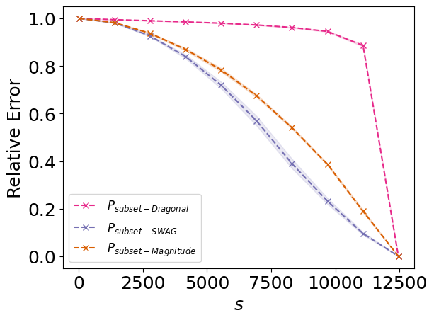
Figure 5: Relative error (20) of the epistemic covariance matrix of the studied subset methods for $s$ up to the number of parameters $p$ for MNIST.

Appendix C Trace Criterion

Ideally we would like to choose a map $P$ such that the predictive distribution of the full (10), (12) and subspace model (18) are as close as possible. Both distributions differ only in their epistemic predictive covariance. Therefore the relative error (20) is a good measure to validate the quality of $P$. However, in practice the relative error cannot be computed because the full covariance matrix is unknown.

As an alternative criterion we propose for our purposes to use the trace $\operatorname{Tr}\Sigma_{P,X}$ instead. This criterion is feasible to compute, aligns well with the relative error as we show empirically in Section 5 and can be motivated by the following lemma:

Lemma 2.

For any $P\in\mathbb{R}^{p\times s}$ we have

$$\Sigma_{P,X}\preccurlyeq\Sigma_{X}$$ (28)

in the Loewner ordering, i.e. $\Sigma_{X}-\Sigma_{P,X}$ is positive semi-definite. In particular we have

$$\operatorname{Tr}\Sigma_{P,X}\leq\operatorname{Tr}\Sigma_{X}\,.$$ (29)

Proof.

Due to the identities (11) and (19) it suffices to show that $P\left(P^{\intercal}\Psi^{-1}P\right)^{-1}P^{\intercal}\preccurlyeq\Psi$, i.e. that the matrix

$$\Psi-P(P^{\intercal}\Psi^{-1}P)^{-1}P^{\intercal}=\Psi^{1/2}(\mathbb{1}-B)\Psi^{1/2}$$

is positive definite, where we introduced $B=W\left(W^{\intercal}W\right)^{-1}W^{\intercal}$ with $W=\Psi^{-1/2}P$. It’s easy to check that $B$ is a projection ($B^{2}=B$ and $B^{\intercal}=B$) which thus has only eigenvalues contained in $\{0,1\}$. From this it follows that $\mathbb{1}-B$ and $\Psi^{1/2}(\mathbb{1}-B)\Psi^{1/2}$ is positive semi-definite and thus (28).

From (28) we obtain $\operatorname{Tr}(\Sigma_{X}-\Sigma_{P,X})=\operatorname{Tr}\Sigma_{X}-\operatorname{Tr}\Sigma_{P,X}\geq 0$ from which (29) follows. ∎

The relation (29) shows that $\operatorname{Tr}(\Sigma_{X}-\Sigma_{P,X})\geq 0$ is a non-negative quantity that quantifies the closeness between $\Sigma_{X}$ and $\Sigma_{P,X}$. Since $\Sigma_{X}$ does not depend on $P$ we can judge whether for two $P_{1},P_{2}$ we have $\operatorname{Tr}(\Sigma_{X}-\Sigma_{P_{1},X})\geq\operatorname{Tr}(\Sigma_{X}-\Sigma_{P_{2},X})$ by simply comparing whether $\operatorname{Tr}\Sigma_{P_{1},X}\geq\operatorname{Tr}\Sigma_{P_{2},X}$. In other words, we can take $\operatorname{Tr}{\Sigma_{P,X}}$ to rank the quality of different $P$. Relation (29) ensures that there is an upper bound for this quantity. We observe in Section 5 empirically that a greater value of the trace implies a lower relative error, which motivates the usage of $\operatorname{Tr}\Sigma_{P,X}$ further. Recall that the trace is the sum of all eigenvalues of a matrix. If the trace of one approximation is greater than another one, it means that this affine subspace covers an eigenspace of greater eigenvalues.

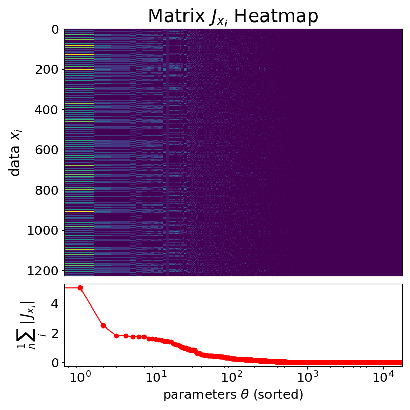
(a) ENB

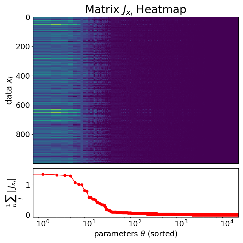
(b) California

Figure 6: The top displays a heatmap which highlights the activity of the gradients corresponding to the parameter $\theta_{i}$. The parameters are sorted according to their sensitivity. A dark bluish colour implies that the gradient w.r.t. the data point $x_{i}$ is negligible. The lower plot summarizes the magnitude of the sensitivity over all data points.

Appendix D MNIST for Large $s$

In Figure 2 it appears that the subset projection matrices $P_{\mathrm{subset-Magnitude}},P_{\mathrm{subset-Diagonal}}$ and $P_{\mathrm{subset-SWAG}}$ fail to approximate the epistemic covariance matrix $\Sigma_{X}$ that is obtained from the Laplace approximation. However, this is misleading. In contrast, Figure 5 reveals that if a sufficient amount of parameters is selected, the subset methods approximate $\Sigma_{X}$ arbitrary well. This has to be expected because in the limiting case that all parameters are selected the projector for these methods is the identity map. But Figure 5 shows that the subset methods cannot provide a reliable approximation of $\Sigma_{X}$ for small $s$. All subset methods require more than one thousand parameters to lead to a slight improvement in the relative error and to achieve a significant reduction more than 9000 out of 12458 parameters are needed (cf. Table 4). Hence, for a selection of few parameters all subset methods fail.

Appendix E Dead Parameters

dataset	ENB	Wine	California	Naval
dead $p$	$92\pm 1\%$	$89\pm 2\%$	$60\pm 2\%$	$34\pm 4\%$

Table 6: Relative number of parameters $p$ that are insensitive to the input data with standard deviation over five seeds.

Even though there is no guarantee that the approximated low rank methods provide better solutions as the subset methods, we would still expect that, in general, they do, because they allow for linear combinations of the parameters instead of a simple selection. In particular, all subset solutions could be found by the low rank approximations, however, the opposite isn’t possible. One reason why subset methods could outperform low rank methods is that most of the parameters are irrelevant for a certain problem, i.e. have a gradient of zero w.r.t. the input. Indeed, Table 6 confirms this hypotheses, because the number of insensitive parameters positively correlates with an improved performance of the subset methods compared to the low rank methods. ENB is the only experiment in which the selection subspace models are superior to the low rank subspace models, but it also the model with most insensitive parameters. Further, for California or Naval Propulsion low rank approximations clearly outperform subset approximations (cf. Figure 1).

This effect is visualized in Figure 6. The top displays a heatmap that highlights the sensitivity of parameters (the gradient w.r.t. the input) for a certain data point. Light colours denote high sensitivity and dark colours low sensitivity. Below the average gradient of all data points w.r.t. a certain parameter is shown. Both plots indicate that only a few parameters are responsive for most data points. According to Table 6, for ENB the used neural network has the least amount of sensitive parameters. If a subset method can capture these parameters, it shall perform well. In contrast, for California the sensitivity is more spread and hence, a linear combination could be more appropriate.

Appendix F NLL

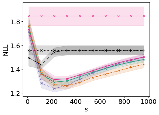
(a) ENB

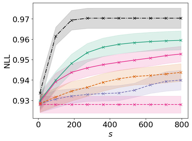
(b) Red Wine

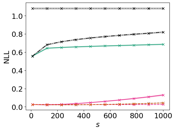
(c) MNIST

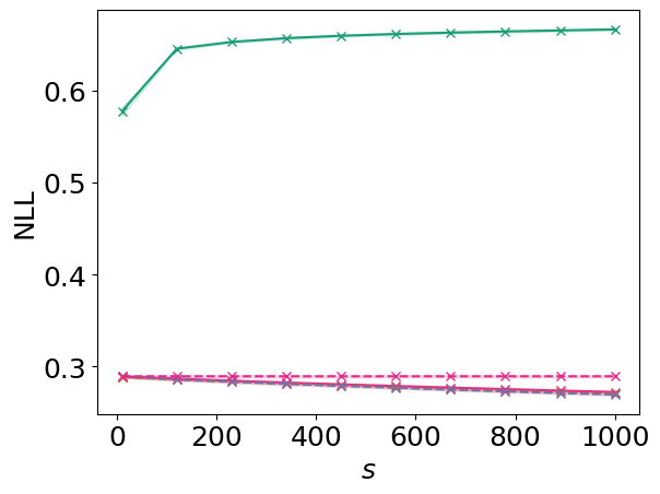
(d) CIFAR10

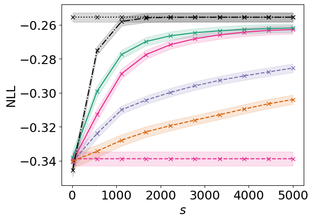
(e) California

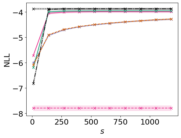
(f) Naval Propulsion

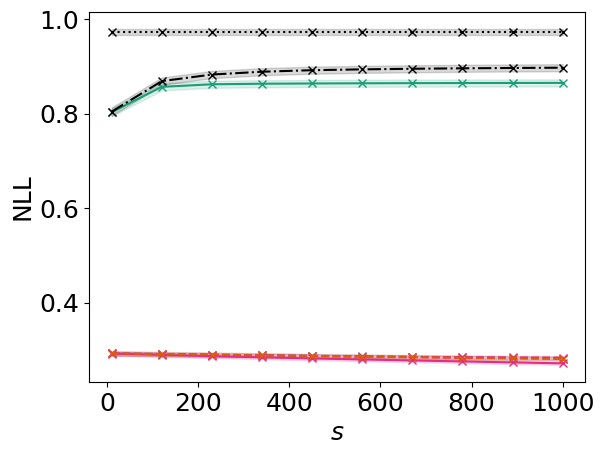
(g) FashionMNIST

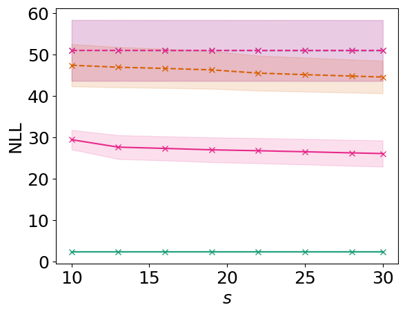
(h) ImageNet10

Figure 7: The NLL metric (30) for the datasets and subspace models considered in this work. The colour and linestyle coding is identical to the one in Figure 1.

The NLL (negative log-likelihood) is a common metric used in the literature [4, 49, 3, 5, 23, 24] to evaluate uncertainties associated with the predictions of (Bayesian) neural networks. The NLL metric is actually the averaged negative logarithm of the posterior predictive distribution (9) on the test data, that is

$$\mathrm{NLL}=-\frac{1}{N_{\mathrm{test}}}\ln p(Y_{\mathrm{test}}|X_{\mathrm{test}},\mathcal{D})\,,$$ (30)

where $X_{\mathrm{test}}$ and $Y_{\mathrm{test}}$ denote the inputs and labels for the $N_{\mathrm{test}}$ test data points. While the NLL is easy to compute for most uncertainty evaluations, there is some criticism that it is not really measuring the real objective but rather something different [50, 51]. Our observations fall in line with these arguments.

Figure 7 shows the results of the NLL for all datasets considered in this work. Recall that a lower NLL is supposed to indicate a superior model. Following this logic most plots in Figure 7 would indicate a reverse ranking of the subspace models compared to the one observed with the relative error and trace criterion in Figure 1 and Figure 2. One might argue, that this could demonstrate that the relative error and trace criterion are unsuitable for evaluating our models. However, it seems unlikely that a criterion such as the relative error that uses information of the full model yields an inferior evaluation of the considered models as a criterion such as the NLL that does not. Moreover, there are two observation in Figure 7 that raises considerable doubt on the NLL ranking:

1. First, note that for most models the NLL rises with increasing $s$. In other words, the NLL evaluates subspace models that use less parameters as better.

2. Second, the full model has the highest NLL value. In other words the NLL ranks it as the worst performing model, whereas the models that approximate it perform better under this metric.

It seems rather implausible that an approximated object yields preciser estimates than the object which it approximates. We feel therefore save to conclude that the ranking obtained via the NLL is unsuitable for our purposes.

Observation 1 was not made in [24], which is the only reference we could find with a comparable plot of the NLL over a range of $s$. We found that their scaling of the prior precision $\lambda_{s}=\frac{s}{p}\lambda$ can lead to a decrease of the NLL but this seems to root in the effect that this scaling tends to decrease the full posterior variance with increasing $s$ (as can be observed, e.g., via the trace of the posterior predictive variance).

To better understand why a misleading behaviour of the NLL as in Observation 1 can occur, let us look at a 1D regression problem (1D input and 1D output) with homoscedastic noise. To simplify the theoretical discussion let us further assume an input independent epistemic predictive covariance $\Sigma\geq 0$ (which is a scalar for the considered problems). The NLL is then given by

$$\mathrm{NLL}(\Sigma)= \frac{1}{2N_{\mathrm{test}}(\sigma^{2}+\Sigma)}\sum_{i=1}^{N_{\mathrm{test}}}(y_{i}-f_{\hat{\theta}}(x_{i}))^{2}$$

$$+\frac{1}{2}\ln(2\pi(\Sigma+\sigma^{2})).$$

It is easy to check that this is a concave function with a global minimum that is dependent on the MSE on the test data:

$$\operatorname*{arg\,min}_{\Sigma}\mathrm{NLL}(\Sigma)=\mathrm{MSE}_{\mathrm{test}}-\sigma^{2}\,.$$ (31)

In standard problems the label noise $\sigma^{2}$ is unknown and needs to be estimated. The standard way of doing this [1, 24, 23] is to learn $\sigma$ as an extra parameter while training. But this leads to an estimate $\hat{\sigma}^{2}=\mathrm{MSE}_{\mathrm{train}}\simeq\mathrm{MSE}_{\mathrm{test}}$ (provided there is no substantial overfitting). As a consequence the NLL (31), computed with $\hat{\sigma}$ instead of $\sigma$, will due to (31) obtain its minimum around $\Sigma=0$. In other words, independent of the problem, fit quality and actual model error, the NLL will rank smaller model uncertainties better.

To exemplify this, Figure 8 shows the results for a synthetic regression dataset with regression function $g(x)=\sin(x/4)\cdot\cos(x/2)$ (Fig. 8(a)) and noise $\sigma=0.1$. In Figure 8(b) the NLL metric is plotted for the methods used in this work when $\sigma$ is estimated ($\hat{\sigma}\simeq 0.23$). We recognize the familiar rise of the NLL with increasing $s$ already observed in Figure 7. When the true $\sigma$ is used instead, the behaviour gets more complicated as can be seen in Figure 8(c). Figure 8(d) shows the behaviour of the subset methods over a longer range of $s$. In Figure 8(c) and 8(d) we see the concave behaviour of the NLL postulated above. The NLL reaches a minimum before it rises to the NLL of the full model. The studied low rank and subset methods achieve a similar minimal value for the NLL, but at different $s_{0}$ that depend on the chosen method. Observation 2 still holds and the full model is outperformed by its approximations. This indicates that even when $\sigma$ is known the usage of the NLL for the assessment of subspace models as studied in this work is questionable.

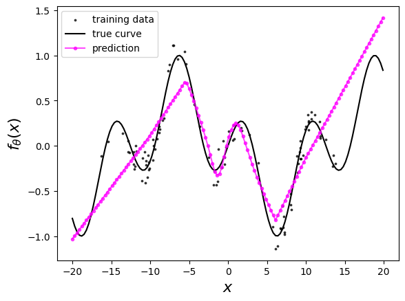
(a) Synthetic dataset

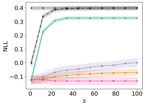
(b) NLL with estimated $\hat{\sigma}$

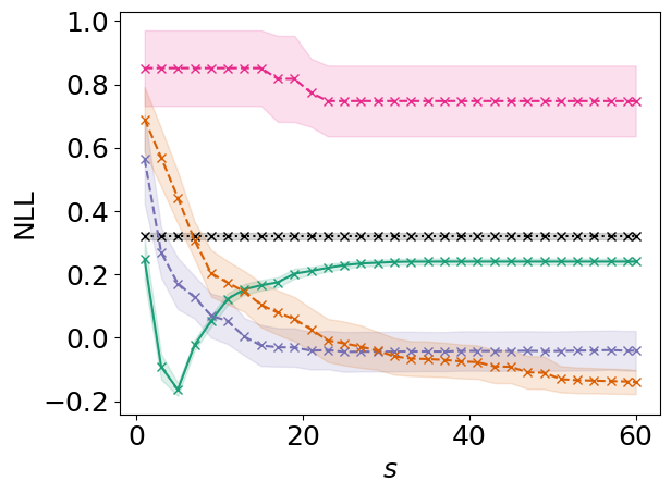
(c) NLL with true $\sigma$

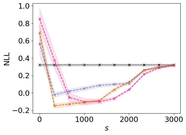
(d) NLL with true $\sigma$

Figure 8: Figure 8(a) visualizes the prediction quality of the parametric function $f_{\theta}$ in comparison to the true curve $g$. The following Figures 8(b) - 8(c) study the NLL for different data variances. In Figure 8(b) the NLL for the estimated data variance $\hat{\sigma}>\sigma=0.1$ is studied. All NLL curves increase with $s$. Adding the epistemic covariance increases the total variance, however, this leads to an increase to the NLL. In contrast, if the true $\sigma$ is taken the NLL is concave. Colour and line encoding are the same as in Figure 1.

Appendix G Fisher Information, Generalized Gauss Newton and Hessian

The Fisher information matrix, generalized Gauss-Newton matrix and Hessian are closely related and in certain situations they are even equivalent. We summarize some of these relations, but for a more detailed analyses we refer to the excellent survey [18].

In supervised machine learning the data is usually distributed by a joint distribution $q(x,y)=q(y|x)q(x)$ which is often unknown. Only the empirical data distribution $\hat{q}(x,x)=\hat{q}(y|x)\hat{q}(x)$ is given in form of samples. The task of supervised machine learning is to learn a parametric distribution $p(x,y|\theta)=p(y|x,\theta)q(x)$ that approximates $q(x,y)$. Since only the conditional distribution $p(y|x,\theta)$ is learned, $q(x,y)$ and $p(x,y|\theta)$ have the same marginal distribution in $x$.

G.1 Fisher Information

G.1.1 Multivariate Regression

$$p(y_{i}|x_{i},\theta)=\frac{1}{\sqrt{(2\pi)^{C}\det(\Sigma)}}e^{-\frac{1}{2}\lVert y_{i}-f(x_{i},\theta)\rVert^{2}_{\Sigma^{-1}}}$$

is a common choice to model multivariate regression problems. For simplicity we assume that the covariance matrix $\Sigma\in\mathbb{R}^{C\times C}$ is independent of the parameter $\theta$. The explicit form of the information matrix for a single input $x_{i}$ is

$$\begin{split}\mathcal{I}_{kl}(x_{i})&=\frac{1}{2}\mathbb{E}_{y\sim p(y|x_{i},\theta)}\left[\partial_{\theta_{k}}\partial_{\theta_{l}}\lVert y_{i}-f_{i}\rVert^{2}_{\Sigma^{-1}}\right]\\ &=\sum_{c_{1},c_{2}=1}^{C}\partial_{\theta_{k}}f_{i}^{c_{1}}\left(\Sigma^{-1}\right)^{c_{1}c_{2}}\partial_{\theta_{l}}f^{c_{2}}_{i}\\ &=\left(\left(\nabla_{\theta}f_{i}\right)^{\intercal}\Sigma^{-1}\nabla_{\theta}f_{i}\right)_{kl}\,.\end{split}$$ (32)

The abbreviation $f_{i}=f_{\theta}(x_{i})$ is used for readability. For $\Sigma=\sigma^{2}\mathbb{1}$ (as in this work), we obtain

$$\begin{split}\mathcal{I}_{kl}(x_{i})=\sigma^{-2}\left(\left(\nabla_{\theta}f_{i}\right)^{\intercal}\nabla_{\theta}f_{i}\right)_{kl}\,.\end{split}$$

For the Fisher information matrix of the joint distribution we arrive at

$$\begin{split}\mathcal{I}_{kl}&=\frac{1}{2}\mathbb{E}_{(x,y)\sim p(y,x|\theta)}\left[\partial_{\theta_{k}}\partial_{\theta_{l}}\lVert y_{i}-f_{i}\rVert^{2}_{\sigma^{-2}\mathbb{1}}\right]\\ &\simeq\frac{\sigma^{-2}}{N}\sum_{i=1}^{N}\left(\left(\nabla_{\theta}f_{i}\right)^{\intercal}\nabla_{\theta}f_{i}\right)_{kl}\,.\end{split}$$

where in the last line $q(x)$ is approximated by $\hat{q}(x)$.

G.1.2 Softmax Classifier

For classification we consider the categorical distribution $y|x,\theta\sim\mathrm{Cat}(y|\phi(f_{\theta}(x))$ with probability vector

$$\phi^{c}_{i}=\phi^{c}(f_{\theta}(x_{i}))=\frac{e^{f_{\theta}^{c}(x_{i})}}{\sum_{\tilde{c}=1}^{C}e^{f^{\tilde{c}}_{\theta}(x_{i})}}=\frac{e^{f^{c}_{i}}}{\sum_{\tilde{c}=1}^{C}e^{f^{\tilde{c}}_{i}}}.$$

The general form of the Fisher information matrix is given by

$$\begin{split}\mathcal{I}_{kl}&=\mathbb{E}_{(x,y)\sim p(x,y|\theta)}\left[\partial_{\theta_{k}}\ln p(x,y|\theta)\partial_{\theta_{l}}\ln p(x,y|\theta)\right]\\ &=\mathbb{E}_{y\sim p(y|x,\theta),x\sim q(x)}\left[\partial_{\theta_{k}}\ln p(y|x,\theta)\partial_{\theta_{l}}\ln p(y|x,\theta)\right]\\ &\simeq\frac{1}{N}\sum_{i=1}^{N}\sum_{c=1}^{C}\phi^{c}_{i}\partial_{\theta_{k}}\ln\phi^{c}_{i}\partial_{\theta_{l}}\ln\phi^{c}_{i}\\ &=\frac{4}{N}\sum_{i=1}^{N}\sum_{c=1}^{C}\partial_{\theta_{k}}\sqrt{\phi^{c}_{i}}\partial_{\theta_{l}}\sqrt{\phi^{c}_{i}}\,,\end{split}$$

where in the third line the empirical distribution $\hat{q}(x)$ is used to compute the expected value of the random variable $x$.

G.2 Relation Between Hessian and Fisher Information Matrix

Given the averaged log-likelihood $\frac{1}{N}\sum_{i}\ln p(y_{i}|f_{\theta}(x_{i}))$ of the data its Hessian w.r.t $\theta$ can be written as

$$\begin{split}H&=-\frac{1}{N}\sum_{i=1}^{N}\nabla^{2}_{\theta}\ln p(y_{i}|f_{\theta}(x_{i}))\\ &=\mathbb{E}_{(x,y)\sim\hat{q}(x,y)}\left[H_{\text{-}\ln p(y|x,\theta)}\right]\\ &=\frac{1}{N}\sum_{i=1}^{N}\mathbb{E}_{y\sim\hat{q}(y|x_{i})}\left[H_{\text{-}\ln p(y|x_{i},\theta)}\right]\,,\end{split}$$ (33)

where we wrote $H_{\text{-}\ln p(y|x,\theta)}=-\nabla^{2}_{\theta}\ln p(y|f_{\theta}(x))$.

The Fisher information matrix $\mathcal{I}$ of $p(x,y|\theta)$ w.r.t the parameter $\theta$ is

$$\begin{split}\mathcal{I}&=\mathbb{E}_{(x,y)\sim p(x,y|\theta)}\left[\nabla_{\theta}\ln p(x,y|\theta)^{\intercal}\nabla_{\theta}\ln p(x,y|\theta)\right]\\ &=\mathbb{E}_{y\sim p(y|x,\theta),x\sim q(x)}\left[\nabla_{\theta}\ln p(y|x,\theta)^{\intercal}\nabla_{\theta}\ln p(y|x,\theta)\right]\\ &=-\mathbb{E}_{y\sim p(y|x,\theta),x\sim q(x)}\left[\nabla_{\theta}^{2}\ln p(y|x,\theta)\right]\\ &=\mathbb{E}_{y\sim p(y|x,\theta),x\sim q(x)}\left[H_{\text{-}\ln p(y|x,\theta)}\right]\,.\end{split}$$

Since $q(x)$ is not analytically known, we shall use the empirical distribution $\hat{q}(x)$ instead.

$$\begin{split}\mathcal{I}=\frac{1}{N}\sum_{i=1}^{N}\mathbb{E}_{y\sim p(y|x=x_{i},\theta)}\left[H_{\text{-}\ln p(y|x,\theta)}\right]\,.\end{split}$$ (34)

The equations (34) and (33) are quite similar. The difference is the distribution under which the expectation is computed. However, note that (33) and (34) are different from the empirical Fisher information matrix

$$\begin{split}\mathcal{I_{\mathrm{empirical}}}&=\mathbb{E}_{y\sim\hat{q}(x,y|\theta)}\left[\nabla_{\theta}\ln p(x,y|\theta)^{\intercal}\nabla_{\theta}\ln p(x,y|\theta)\right]\\ &=\frac{1}{N}\sum_{i=1}^{N}\nabla_{\theta}\ln p(y_{i}|x_{i},\theta)^{\intercal}\nabla_{\theta}\ln p(y_{i}|x_{i},\theta).\end{split}$$

G.3 Relation Between Hessian and Generalized Gauss-Newton Matrix

The generalized Gauss-Newton matrix is often used as a substitute of the Hessian because it is positive semi-definite and easier to compute [18]. For generalized linear models both quantities coincide. Let us write the Jacobian w.r.t. the log-likelihood as $\nabla_{\theta}\ln p(y_{i}|f_{\theta}(x_{i}))=\nabla_{f_{i}}\ln p(y_{i}|f_{i})\nabla_{\theta}f_{\theta}(x_{i})=\nabla_{f_{i}}\ln p(y_{i}|f_{i})J_{f_{i}}$ and $H_{f_{i}^{c}}=\nabla_{\theta}^{2}f_{\theta}(x_{i})^{c}$ for $1\leq c\leq C$. Then the Hessian can be decomposed into

$$\begin{split}H=&\frac{-1}{N}\sum_{i=1}^{N}\Big{(}J_{f_{i}}^{\intercal}\nabla_{f_{i}}^{2}\ln p(y_{i}|f_{i})J_{f_{i}}\\ &+\sum_{c=1}^{C}H_{f_{i}^{c}}\partial_{f_{i}^{c}}\ln p(y_{i}|f_{i})\Big{)}\\ =&H_{\mathrm{GGN}}-\frac{1}{N}\sum_{i=1}^{N}\sum_{c=1}^{C}H_{f_{i}^{c}}\partial_{f_{i}^{c}}\ln p(y_{i}|f_{i})\end{split}$$ (35)

with the generalized Gauss-Newton matrix

$$\begin{split}H_{\mathrm{GGN}}&=-\frac{1}{N}\sum_{i=1}^{N}J_{f_{i}}^{\intercal}\nabla_{f_{i}}^{2}\ln p(y_{i}|f_{i})J_{f_{i}}\\ &=\frac{1}{N}\sum_{i=1}^{N}J_{f_{i}}^{\intercal}H_{\text{-}\ln p(y_{i}|{f_{i}})}J_{f_{i}}\,.\end{split}$$ (36)

A sufficient condition that the generalized Gauss-Newton matrix and the Hessian coincide is that the model is linear, because for linear models $H_{f_{i}^{c}}=0$ for $1\leq c\leq C$. In the definition of the generalized Gauss-Newton matrix a choice about where the cut between the loss and the network function has to be made. This is to some degree arbitrary, however, [16] recommends to perform as much as possible of the computation in the loss such that $\ln p(y_{i}|f)$ is still convex to ensure positive semi-definiteness of $H_{\mathrm{GGN}}$.

G.4 Relation Between Fisher Information Matrix and Generalized Gauss-Newton Matrix

Rewriting $\nabla_{\theta}\ln p(y_{i}|f_{\theta}(x_{i}))=\nabla_{f_{i}}\ln p(y_{i}|f_{i})J_{f_{i}}$ the Fisher information matrix is of the form

$$\begin{split}\mathcal{I}&=\mathbb{E}_{y\sim p(y|x,\theta),x\sim q(x)}\left[\nabla_{\theta}\ln p(y|x,\theta)^{\intercal}\nabla_{\theta}\ln p(y|x,\theta)\right]\\ &=\mathbb{E}_{x}\left[J_{f}^{\intercal}\mathbb{E}_{y}\left[\nabla_{f}\ln p(y|f)^{\intercal}\left(\nabla_{f}\ln p(y|f)\right)\right]J_{f}\right]\\ &:=\mathbb{E}_{x}\left[J_{f}^{\intercal}\mathcal{I}_{\ln p(y|f)}J_{f}\right]\,,\end{split}$$ (37)

where we write shorthand $f=f_{\theta}(x)$ and

$$\begin{split}\mathcal{I}_{\ln p(y|f)}&=\mathbb{E}_{y}\left[\nabla_{f}\ln p(y|f)^{\intercal}\nabla_{f}\ln p(y|f)\right]\\ &=-\mathbb{E}_{y}\left[\nabla_{f}^{2}\ln p(y|f)\right]\\ &=\mathbb{E}_{y}\left[H_{\text{-}\ln p(y|f)}\right]\end{split}$$

is the “Fisher information matrix of the predictive distribution”.

From these two identities it easily follows that if we substitute $q(x)$ by its empirical distribution $\hat{q}(x)$, the generalized Gauss-Newton matrix (36) is identical to the Fisher information matrix (37) if $H_{\text{-}\ln p(y|f)}$ is constant in $y$. This is the case for squared error loss and cross-entropy loss [35, 17, 18]. Indeed, for squared error loss we have

$$H_{\text{-}\ln p(y|f)}=\nabla_{f}^{2}\frac{1}{2}\lVert f-y\rVert^{2}_{\Sigma^{-1}}=\Sigma^{-1}$$

and for cross-entropy loss we obtain

$$\begin{split}H_{\ln p(y|f);c^{\prime}c^{\prime\prime}}&=\partial_{f^{c^{\prime}}}\partial_{f^{c^{\prime\prime}}}\sum_{c=1}^{C}y^{c}\ln\phi^{c}\\ &=\partial_{f^{c^{\prime}}}\partial_{f^{c^{\prime\prime}}}\sum_{c=1}^{C}y^{c}\ln\frac{e^{f^{c}}}{\sum_{{\tilde{c}}=1}^{C}e^{f^{\tilde{c}}}}\\ &=\partial_{f^{c^{\prime}}}\partial_{f^{c^{\prime\prime}}}\left(\sum_{c=1}^{C}y^{c}f^{c}-\sum_{c}y^{c}\ln\sum_{{\tilde{c}}=1}^{C}e^{f^{\tilde{c}}}\right)\\ &=\partial_{f^{c^{\prime}}}\partial_{f^{c^{\prime\prime}}}\left(\sum_{c=1}^{C}y^{c}f^{c}-\ln\sum_{{\tilde{c}}=1}^{C}e^{f^{\tilde{c}}}\right)\\ &=-\partial_{f^{c^{\prime}}}\partial_{f^{c^{\prime\prime}}}\ln\sum_{{\tilde{c}}=1}^{C}e^{f^{\tilde{c}}}=-\partial_{f^{c^{\prime\prime}}}\phi^{c^{\prime}}\\ &=-\delta_{c^{\prime}c^{\prime\prime}}\phi^{c^{\prime}}+\phi^{c^{\prime}}\phi^{c^{\prime\prime}}\,,\end{split}$$

which are both constant in $y$.

References

- Gal [2016] Yarin Gal. Uncertainty in deep learning. 2016. URL https://www.cs.ox.ac.uk/people/yarin.gal/website/thesis/thesis.pdf.
- Blundell et al. [2015] Charles Blundell, Julien Cornebise, Koray Kavukcuoglu, and Daan Wierstra. Weight uncertainty in neural network. In International Conference on Machine Learning, pages 1613–1622. PMLR, 2015.
- Kendall and Gal [2017] Alex Kendall and Yarin Gal. What uncertainties do we need in Bayesian deep learning for computer vision? arXiv preprint arXiv:1703.04977, 2017.
- Hernández-Lobato and Adams [2015] José Miguel Hernández-Lobato and Ryan Adams. Probabilistic backpropagation for scalable learning of Bayesian neural networks. In International conference on machine learning, pages 1861–1869. PMLR, 2015.
- Maddox et al. [2019] Wesley J Maddox, Pavel Izmailov, Timur Garipov, Dmitry P Vetrov, and Andrew Gordon Wilson. A simple baseline for Bayesian uncertainty in deep learning. Advances in neural information processing systems, 32, 2019.
- Kingma et al. [2015] Diederik P Kingma, Tim Salimans, and Max Welling. Variational dropout and the local reparameterization trick. arXiv preprint arXiv:1506.02557, 2015.
- Jordan et al. [1999] Michael I. Jordan, Zoubin Ghahramani, T. Jaakkola, and Lawrence K. Saul. An introduction to variational methods for graphical models. Machine Learning, 37:183–233, 1999.
- Wainwright and Jordan [2008] Martin J. Wainwright and Michael I. Jordan. Graphical models, exponential families, and variational inference. Found. Trends Mach. Learn., 1:1–305, 2008.
- MacKay [1992a] David John Cameron MacKay. A practical Bayesian framework for backpropagation networks. Neural Computation, 4:448–472, 1992a.
- LeCun et al. [1989] Yann LeCun, John Denker, and Sara Solla. Optimal brain damage. Advances in neural information processing systems, 2, 1989.
- Ritter et al. [2018] Hippolyt Ritter, Aleksandar Botev, and David Barber. A scalable Laplace approximation for neural networks. In International Conference on Learning Representations, 2018.
- Daxberger et al. [2021a] Erik A. Daxberger, Agustinus Kristiadi, Alexander Immer, Runa Eschenhagen, M. Bauer, and Philipp Hennig. Laplace redux - effortless Bayesian deep learning. In Neural Information Processing Systems, 2021a.
- Dauphin et al. [2014] Yann N. Dauphin, Razvan Pascanu, Çaglar Gülçehre, Kyunghyun Cho, Surya Ganguli, and Yoshua Bengio. Identifying and attacking the saddle point problem in high-dimensional non-convex optimization. arXiv preprint: 1406.2572, 2014. URL http://arxiv.org/abs/1406.2572.
- Sagun et al. [2016] Levent Sagun, Léon Bottou, and Yann LeCun. Eigenvalues of the Hessian in deep learning: Singularity and beyond. arXiv preprint: 1611.07476, 2016. URL https://arxiv.org/abs/1611.07476.
- Papyan [2018] Vardan Papyan. The full spectrum of deepnet Hessians at scale: Dynamics with sgd training and sample size. arXiv preprint: 1811.07062, 2018. URL https://arxiv.org/abs/1811.07062.
- Schraudolph [2002] Nicol N. Schraudolph. Fast Curvature Matrix-Vector Products for Second-Order Gradient Descent. Neural Computation, 14(7):1723–1738, 07 2002. ISSN 0899-7667. doi: 10.1162/08997660260028683.
- Pascanu and Bengio [2013] Razvan Pascanu and Yoshua Bengio. Revisiting natural gradient for deep networks. arxiv preprint: 1301.3584, 2013.
- Martens [2014] James Martens. New insights and perspectives on the natural gradient method. arxiv preprint: 1412.1193, 2014. URL http://arxiv.org/abs/1412.1193.
- Salimans and Kingma [2016] Tim Salimans and Diederik P. Kingma. Weight normalization: A simple reparameterization to accelerate training of deep neural networks. arXiv preprint: 1602.07868, 2016. URL https://arxiv.org/abs/1602.07868.
- Kirkpatrick et al. [2017] James Kirkpatrick, Razvan Pascanu, Neil Rabinowitz, Joel Veness, Guillaume Desjardins, Andrei A Rusu, Kieran Milan, John Quan, Tiago Ramalho, Agnieszka Grabska-Barwinska, et al. Overcoming catastrophic forgetting in neural networks. Proceedings of the national academy of sciences, 114(13):3521–3526, 2017.
- Kristiadi et al. [2020] Agustinus Kristiadi, Matthias Hein, and Philipp Hennig. Being Bayesian, even just a bit, fixes overconfidence in relu networks. arXiv preprint: 2002.10118, 2020. URL https://arxiv.org/abs/2002.10118.
- Snoek et al. [2015] Jasper Snoek, Oren Rippel, Kevin Swersky, Ryan Kiros, Nadathur Satish, Narayanan Sundaram, Md. Mostofa Ali Patwary, Prabhat, and Ryan P. Adams. Scalable Bayesian optimization using deep neural networks. arXiv preprint: 1502.05700, 2015. URL https://arxiv.org/abs/1502.05700.
- Izmailov et al. [2019] Pavel Izmailov, Wesley J. Maddox, Polina Kirichenko, Timur Garipov, Dmitry P. Vetrov, and Andrew Gordon Wilson. Subspace inference for Bayesian deep learning. arxiv preprint: 1907.07504, 2019.
- Daxberger et al. [2021b] E. Daxberger, E. Nalisnick, J. Allingham, J. Antorán, and J. M. Hernández-Lobato. Bayesian deep learning via subnetwork inference. In Proceedings of 38th International Conference on Machine Learning (ICML), volume 139 of Proceedings of Machine Learning Research, pages 2510–2521. PMLR, July 2021b. URL https://proceedings.mlr.press/v139/daxberger21a.html.
- Sharma et al. [2023] Mrinank Sharma, Sebastian Farquhar, Eric Nalisnick, and Tom Rainforth. Do Bayesian neural networks need to be fully stochastic? arxiv preprint: 2211.06291, 2023. URL https://arxiv.org/abs/2211.06291.
- Cheng et al. [2017] Yu Cheng, Duo Wang, Pan Zhou, and Zhang Tao. A survey of model compression and acceleration for deep neural networks. ArXiv, abs/1710.09282, 2017.
- Foong et al. [2019] Andrew Y. K. Foong, Yingzhen Li, José Miguel Hernández-Lobato, and Richard E. Turner. ’in-between’ uncertainty in Bayesian neural networks. arXiv preprint: 1906.11537, 2019. URL https://arxiv.org/abs/1906.11537.
- Immer et al. [2021] Alexander Immer, Maciej Korzepa, and Matthias Bauer. Improving predictions of Bayesian neural nets via local linearization. arXiv preprint: 2008.08400, 2021. URL https://arxiv.org/abs/2008.08400.
- Deng et al. [2022] Zhijie Deng, Feng Zhou, and Jun Zhu. Accelerated linearized Laplace approximation for Bayesian deep learning. ArXiv, abs/2210.12642, 2022.
- Ortega et al. [2023] Luis A. Ortega, Simón Rodríguez Santana, and Daniel Hern’andez-Lobato. Variational linearized Laplace approximation for Bayesian deep learning. ArXiv, abs/2302.12565, 2023.
- MacKay [1992b] David John Cameron MacKay. The evidence framework applied to classification networks. Neural Computation, 4:720–736, 1992b.
- Botev et al. [2017] Aleksandar Botev, Hippolyt Ritter, and David Barber. Practical Gauss-Newton optimisation for deep learning. In International Conference on Machine Learning, 2017.
- Martens and Grosse [2015] James Martens and Roger Baker Grosse. Optimizing neural networks with Kronecker-factored approximate curvature. In International Conference on Machine Learning, 2015.
- Calvo-Ordonez et al. [2024] Sergio Calvo-Ordonez, Matthieu Meunier, Francesco Piatti, and Yuantao Shi. Partially stochastic infinitely deep Bayesian neural networks. arxiv preprint: 2402.03495, 2024. URL https://arxiv.org/abs/2402.03495.
- Heskes [2000] Tom M. Heskes. On natural learning and pruning in multilayered perceptrons. Neural Computation, 12:881–901, 2000.
- Bishop [2007] Christopher M. Bishop. Pattern recognition and machine learning, 5th Edition. Information science and statistics. Springer, 2007. ISBN 9780387310732. URL https://www.worldcat.org/oclc/71008143.
- Schmidt [1907] Erhard Schmidt. Zur Theorie der linearen und nichtlinearen Integralgleichungen. Mathematische Annalen, 63(4):433–476, Dec 1907. ISSN 1432-1807. doi: 10.1007/BF01449770. URL https://doi.org/10.1007/BF01449770.
- Eckart and Young [1936] Carl Eckart and Gale Young. The approximation of one matrix by another of lower rank. Psychometrika, 1(3):211–218, Sep 1936. ISSN 1860-0980. doi: 10.1007/BF02288367. URL https://doi.org/10.1007/BF02288367.
- Mirsky [1960] L. Mirsky. Symmetric gauge functions and unitarily invariant norms. The Quarterly Journal of Mathematics, 11(1):50–59, 01 1960. ISSN 0033-5606. doi: 10.1093/qmath/11.1.50. URL https://doi.org/10.1093/qmath/11.1.50.
- Vanschoren et al. [2013] Joaquin Vanschoren, Jan N. van Rijn, Bernd Bischl, and Luis Torgo. Openml: Networked science in machine learning. SIGKDD Explorations, 15(2):49–60, 2013. doi: 10.1145/2641190.2641198. URL http://doi.acm.org/10.1145/2641190.2641198.
- [41] Matthias Feurer, Jan N. van Rijn, Arlind Kadra, Pieter Gijsbers, Neeratyoy Mallik, Sahithya Ravi, Andreas Mueller, Joaquin Vanschoren, and Frank Hutter. OpenML-Python: an extensible Python API for OpenML. arXiv, 1911.02490. URL https://arxiv.org/pdf/1911.02490.pdf.
- LeCun et al. [1998] Yann LeCun, Léon Bottou, Yoshua Bengio, and Patrick Haffner. Gradient-based learning applied to document recognition. Proc. IEEE, 86:2278–2324, 1998.
- Mu and Gilmer [2019] Norman Mu and Justin Gilmer. Mnist-c: A robustness benchmark for computer vision, 2019. URL https://arxiv.org/abs/1906.02337.
- Xiao et al. [2017] Han Xiao, Kashif Rasul, and Roland Vollgraf. Fashion-mnist: a novel image dataset for benchmarking machine learning algorithms. ArXiv, abs/1708.07747, 2017.
- Krizhevsky [2009] Alex Krizhevsky. Learning multiple layers of features from tiny images. Technical report, 2009. https://www.cs.toronto.edu/˜kriz/cifar.html.
- Deng et al. [2009] Jia Deng, Wei Dong, Richard Socher, Li-Jia Li, Kai Li, and Li Fei-Fei. Imagenet: A large-scale hierarchical image database. In 2009 IEEE Conference on Computer Vision and Pattern Recognition, pages 248–255, 2009. doi: 10.1109/CVPR.2009.5206848.
- Paszke et al. [2019] Adam Paszke, Sam Gross, Francisco Massa, Adam Lerer, James Bradbury, Gregory Chanan, Trevor Killeen, Zeming Lin, Natalia Gimelshein, Luca Antiga, Alban Desmaison, Andreas Kopf, Edward Yang, Zachary DeVito, Martin Raison, Alykhan Tejani, Sasank Chilamkurthy, Benoit Steiner, Lu Fang, Junjie Bai, and Soumith Chintala. Pytorch: An imperative style, high-performance deep learning library, 2019.
- He et al. [2015] Kaiming He, Xiangyu Zhang, Shaoqing Ren, and Jian Sun. Deep residual learning for image recognition. arXiv preprint arXiv:1512.03385, 2015. URL http://arxiv.org/abs/1512.03385.
- Lakshminarayanan et al. [2017] Balaji Lakshminarayanan, Alexander Pritzel, and Charles Blundell. Simple and scalable predictive uncertainty estimation using deep ensembles. Advances in neural information processing systems, 30, 2017.
- Yao et al. [2019] J. Yao, W. Pan, S. Ghosh, and F. Doshi-Velez. Quality of uncertainty quantification for bayesian neural network inference. 2019.
- Deshpande et al. [2024] Sameer K. Deshpande, Soumya Ghosh, Tin D. Nguyen, and Tamara Broderick. Are you using test log-likelihood correctly? Trans. Mach. Learn. Res., 2024, 2024. URL https://openreview.net/forum?id=n2YifD4Dxo.