Geometric Neural Process Fields
Abstract
This paper addresses the challenge of Neural Field (NeF) generalization, where models must efficiently adapt to new signals given only a few observations. To tackle this, we propose Geometric Neural Process Fields (G-NPF), a probabilistic framework for neural radiance fields that explicitly captures uncertainty. We formulate NeF generalization as a probabilistic problem, enabling direct inference of NeF function distributions from limited context observations. To incorporate structural inductive biases, we introduce a set of geometric bases that encode spatial structure and facilitate the inference of NeF function distributions. Building on these bases, we design a hierarchical latent variable model, allowing G-NPF to integrate structural information across multiple spatial levels and effectively parameterize INR functions. This hierarchical approach improves generalization to novel scenes and unseen signals. Experiments on novel-view synthesis for 3D scenes, as well as 2D image and 1D signal regression, demonstrate the effectiveness of our method in capturing uncertainty and leveraging structural information for improved generalization.
1 Introduction
Neural Fields (NeFs) (Sitzmann et al., 2020b; Tancik et al., 2020) have emerged as a powerful framework for learning continuous, compact representations of signals across domains, including 1D signal (Yin et al., 2022), 2D images (Sitzmann et al., 2020b), and 3D scenes (Park et al., 2019; Mescheder et al., 2019). A notable advancement in 3D scene modeling is Neural Radiance Fields (NeRFs) (Mildenhall et al., 2021; Barron et al., 2021), which extend NeFs to map 3D coordinates and viewing directions to volumetric density and view-dependent radiance. By differentiable volume rendering along camera rays, NeRFs achieve photorealistic novel view synthesis. Although NeRFs achieve good reconstruction performance, they must be overfitted to each 3D object or scene, resulting in poor generalization to new 3D scenes with few context images.
In this paper, we focus on neural field generalization (also referred to as conditional neural fields) and the rapid adaptation of NeFs to new signals. Previous works on NeF generalization have addressed this challenge using gradient-based meta-learning (Tancik et al., 2021), enabling adaptation to new scenes with only a few optimization steps (Tancik et al., 2021; Papa et al., 2024). Other approaches include modulating shared MLPs through HyperNets (Chen & Wang, 2022; Mehta et al., 2021; Dupont et al., 2022a; Kim et al., 2023) or directly predicting the parameters of scene-specific MLPs (Dupont et al., 2021; Erkoç et al., 2023). However, the deterministic nature of these methods cannot capture uncertainty in NeFs, when used with scenes with only limited observations are available. This is important as such sparse data may be interpreted in multiple valid ways.
To address uncertainty arising from having few context images, probabilistic NeFs (Gu et al., 2023; Guo et al., 2023; Kosiorek et al., 2021) have recently been investigated. For example, VNP (Guo et al., 2023) and PONP (Gu et al., 2023) infer the NeFs using Neural Processes (NPs) (Bruinsma et al., 2023; Garnelo et al., 2018b; Wang & Van Hoof, 2020), a probabilistic meta-learning method that models functional distributions conditioned on partial signal observations. These probabilistic methods, however, do not exploit potential structural information, such as the geometric characteristics of signals (e.g., object shape) or hierarchical organization in the latent space (from global to local). Incorporating such inductive biases can facilitate more effective adaptation to new signals from partial observations.
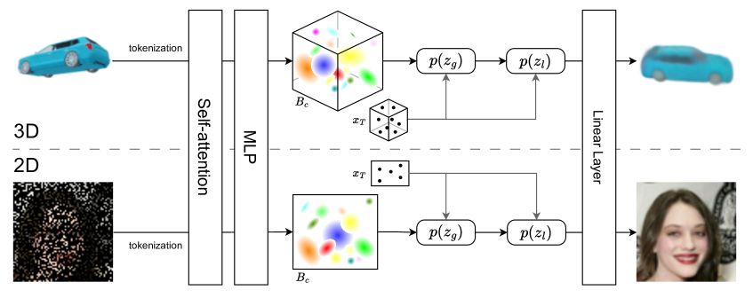
To jointly capture uncertainty and leverage inherent structural information for efficient adaptation to new signals with few observations, we propose a probabilistic neural fields generalization framework called Geometric Neural Processes Fields (G-NPF). Our contributions can be summarized as follows: 1) Probabilistic NeF generalization framework. We formulate NeF generalization as a probabilistic modeling problem, allowing us to amortize a learned model over multiple signals and improve NeF learning and generalization. 2) Geometric bases. To encode structural inductive biases, we design geometric bases that incorporate prior knowledge (e.g., Gaussian structures), enabling the aggregation of local information and the integration of geometric cues. 3) Geometric neural processes with hierarchical latent variables. Building on these geometric bases, we develop geometric neural processes to capture uncertainty in the latent NeF function space. Specifically, we introduce hierarchical latent variables at multiple spatial scales, offering improved generalization for novel scenes and views. Experiments on 1D and 2D signals demonstrate the effectiveness of the proposed method for NeF generalization. Furthermore, we adapt our approach to the formulation of Neural Radiance Fields (NeRFs) with differentiable volume rendering on ShapeNet objects and NeRF Synthetic scenes to validate the versatility of our approach.
2 Background
2.1 Neural (Radiance) Fields
Neural Fields (NeFs) (Sitzmann et al., 2020b) are continuous functions , parameterized by a neural network whose parameters we optimize to reconstruct the continuous signal on coordinates . As with regular neural networks, fitting Neural Field parameters relies on gradient descent minimization. Unlike regular networks, however, conventional Neural Fields are explicitly designed to overfit the signal during reconstruction deterministically, without considering generalization (Mildenhall et al., 2021; Barron et al., 2021). The reason is that Neural Fields have been primarily considered in transductive learning settings in 3D graphics, whereby the optimization objective is to optimally reconstruct the photorealism of single 3D objects at a time. In this case, there is no need for generalization across objects. A single trained Neural Field network is optimized to “fill in” the specific shape of a specific 3D object under all possible view points, given input point cloud (coordinates ). For each separate 3D object, we optimize a separate Neural Field afresh. Beyond 3D graphics, Neural Fields have found applicability in a broad array of 1D (Yin et al., 2022) and 2D (Chen et al., 2023b) applications, for scientific (Raissi et al., 2019) and medical data (de Vries et al., 2023), especially when considering continuous spatiotemporal settings.
Neural Radiance Fields (NeRF) (Mildenhall et al., 2021; Arandjelović & Zisserman, 2021) are Neural Fields specialized for 3D graphics, reconstructing the 3D shape and texture of a single objects. Specifically, each point in the 3D space centered around the object has a color , where is the direction of the camera looking at the point . Since objects might be opaque or translucent, points also have opacity . In Neural Field terms, therefore, our input comprises point coordinates and the camera direction, that is , and our output comprises colors and opacities, that is .
Optimizing a NeRF is an inverse problem: we do not have direct access to ground-truth 3D colors and points of the object. Instead, we optimize solely based on 2D images from known camera positions and viewing directions . Specifically, we optimize the parameters of the NeRF function, which encodes the 3D shape and color of the object, allowing us to render novel 2D views from arbitrary camera positions and directions using ray tracing along . This ray-tracing process integrates colors and opacities along the ray, accumulating contributions from points until they reach the camera. The objective is to ensure that NeRF-generated 2D views match the training images. Since these images provide an object-specific context for inferring its 3D shape and texture, we refer to them as context data. In contrast, all other unknown shape and texture information is target data. For a detailed description of the ray-tracing integration process, see Appendix A.
Conditional Neural Fields (Papa et al., 2024) have recently gained popularity to avoid optimizing from scratch a new Neural Field for every new object. Conditional Neural Fields split parameters to a shared part that is common between objects in the dataset , and an object-specific part that is optimized specifically for the -th object. However, the optimization of is still done independently per object using stochastic gradient descent.
2.2 Neural Processes
Neural Processes (NPs) (Garnelo et al., 2018b; Kim et al., 2019) extend the notion of Gaussian Processes (GPs) (Rasmussen, 2003) by leveraging neural networks for flexible function approximation. Given a context set of input–output pairs, NPs infer a latent variable that captures function-level uncertainty. When presented with new inputs , the goal is to predict . Formally, NPs define the predictive distribution:
| (1) |
Here, is a prior over derived solely from the context set. During training, an approximate posterior (where is the target set consisting of pairs) is learned via variational inference (Garnelo et al., 2018b). Through this latent-variable formulation, NPs capture both predictive uncertainty and function-level variability, enabling robust performance under partial observations.
3 Geometric Neural Process Fields
Despite their great reconstruction capabilities, Neural Fields are still limited by their lack of generalization. While Conditional Neural Fields offer an interesting path forward, they still suffer from the unconstrained nature of stochastic gradient descent and the over-parameterized nature of neural networks (Papa et al., 2024), thus making representation learning and generalization to few-shot settings hard, whether for 1-D (e.g., for time series), 2-D (e.g., for PINNs), or 3-D (e.g., for occupancy and radiance fields) data. We alleviate this by imposing geometric and hierarchical structure to the NeF and NeRF functions in 1-, 2-, or 3-D data, such that Neural Fields are constrained to the types of outputs that they predict. Further, we embed Conditional Neural Fields in a probabilistic learning framework using Neural Processes, so that the learned Neural Fields generalize well even with few-shot context data settings.
3.1 Probabilistic Neural Process Fields
Conditional Neural Fields, defined in a deterministic setting, bear direct resemblance to Neural Processes and Gaussian Processes and their context and target sets, defined in a probabilistic setting. To make the point clearer, we will use the 2D image completion task as a running example, where the goal is to reconstruct an entire image from a sparse set of observed pixels (an occluded image).
In image completion task, the consists of observed pixel coordinates and their corresponding intensity values , while the target set comprises all pixel coordinates in the image, with denoting the unobserved intensities to be predicted. The objective is thus to infer the full image conditioned on , effectively regressing pixel intensities across the entire spatial domain using only the sparse context observations. Although our approach is formulated as a general probabilistic framework, we present a novel 3D-specific extension for Neural Radiance Fields, detailed in Appendix F.
For probabilistic Neural Process Fields, we adopt the Neural Process decomposition from Eq. (1) for prior distribution,
| (2) | ||||
where in the last line of Eq. (2) we use the fact that the target output variables, which comprise the target object, are conditionally independent with respect to the latent variable . In probabilistic Neural Process Fields, encodes object-level information, similar to the object-specific parameters in deterministic Conditional Neural Fields. However, by modeling probabilistically, our approach enables generalization across different objects, whereas standard NeFs are limited to fitting a single object at a time.
3.2 Adding Geometric Priors to Probabilistic Neural Process Fields
With probabilistic Neural Process Fields, we are able to generalize conditional Neural Fields to account for uncertainty and thus be more robust to smaller training datasets and few-shot learning settings. Given that (conditional) Neural Fields are typically implemented as standard MLPs, they do not pertain to a specific structure in their output nor are they constrained in the type of values they can predict. This lack of constraints can have a detrimental impact on the generalization of the learned models, especially when considering Neural Radiance Fields, for which one must also make sure that there is consistency between the 2D observations and the 3D shape of the object.
To address this problem, we propose adding geometric priors to probabilistic Neural Process Fields. Specifically, we encode the context set so that to represent it in terms of structured geometric bases , rather than using directly. Here is the number of bases. These geometric bases must create an information bottleneck through which we embed structure to the context set , thus . Each geometric basis contains a Gaussian distribution in the 2D spatial plane with covariance , centered around a 2D coordinate . Note that when extending to the 3D data, is a 3D Gaussian. Each geometric basis also contains a representation variable , learned jointly to encode the semantics around the location of . The probabilistic Neural Process Field in Eq. (2) becomes
| (3) |
3.3 Adding Hierarchical Priors to Probabilistic Neural Process Fields
The decomposition in Eq. (2) conditioning on the latent allows generalizing conditional Neural Fields with uncertainty to arbitrary training sets, especially by introducing geometric priors in Eq. (3). We note, however, that when learning probabilistic Neural Fields, our training must serve two slightly conflicting objectives. On one hand, the latent variable encodes the global appearance and geometry of the target object at . On the other hand, the Neural Fields are inherently local, in that their inferences are coordinate-specific.
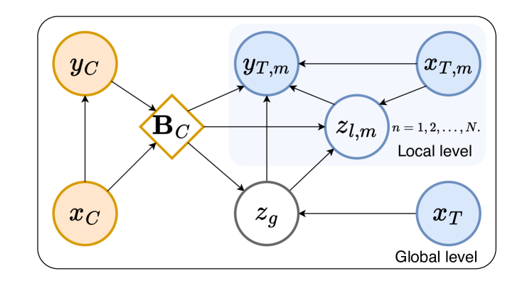
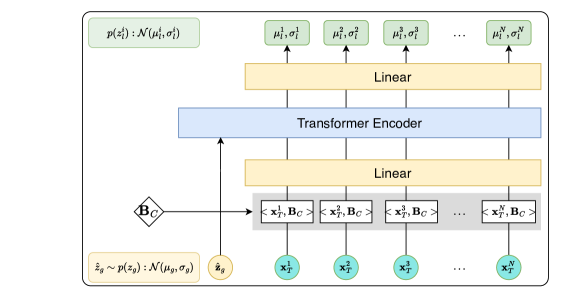
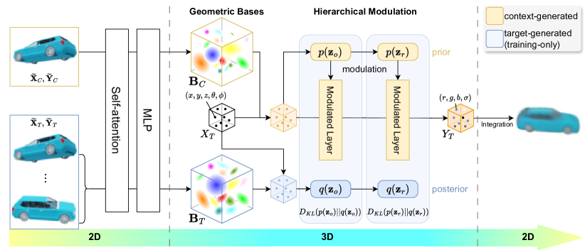
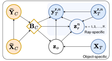
To ease the tension, we introduce hierarchical latent variables, having a single global latent variable , and local latent variables for the target points , to condition the probabilistic Neural Process Fields. A graphical model of our method is provided in Fig. 2.
| (4) | |||
| (5) |
3.4 Implementation
We next describe the implementation of all individual components, and refer to the Appendix C for the full details.
Geometric basis functions.
We implement the geometric basis functions using a transformer encoder, . In of Eq. (5), the prior distribution of each hierarchical latent variable is conditioned on the geometric bases and target inputs . Since the geometric basis functions rely on Gaussians, we use an MLP with a Gaussian radial basis function to measure their interaction, that is
| (6) | ||||
Global latent variables.
We model the global latent variable as a Gaussian distribution:
| (7) |
where is parameterized by a Gaussian whose mean and variance are generated via an MLP. Eq (7) aggregates representations across all target points to produce a global latent variable , thereby parameterizing the underlying object or scene. This formulation enables our model to capture object-specific uncertainty through the inferred distribution of .
Local latent variables.
To infer the distribution of the local latent variables , we first compute the position-aware representation for each target point using Eq (6). The local latent variable is then derived by combining these representations with the global latent variable via a transformer:
where is a sample from the global prior distribution . Mirroring the global latent variable , we model the local prior distribution as a mean-field Gaussian with parameters and . This hierarchical structure enables coordinate-specific uncertainty modeling while preserving global geometric consistency. Full architectural details are provided in Appendix C.2.
Predictive distribution.
The hierarchical latent variables condition the neural network to generate predictions that integrate global and local geometric uncertainty. Specifically, the neural field is conditioned jointly on the global latent variable , which encodes object-level structure, and the local latent variables , which capture coordinate-specific variations. The predictive distribution is obtained by propagating each target coordinate through the neural network, parameterized by and , to model the distribution of outputs . This process directly leverages the hierarchical prior distributions defined in Eq (5), ensuring consistency across scales. Implementation details of the conditioned network are provided in Appendix C.3.
3.5 Training objective
To optimize the proposed G-NPF, we apply variational inference (Garnelo et al., 2018b) to derive the evidence lower bound (ELBO). Specifically, we first introduce the hierarchical variational posterior:
| (8) | ||||
where are target set-derived bases (available only at training). The variational posteriors are inferred from the target set during training with the same encoder, which introduces more information on the object. The prior distributions are supervised by the variational posterior using Kullback–Leibler (KL) divergence, learning to model more object information with limited context data and generalize to new scenes. The details about the evidence lower bound (ELBO) and derivation are provided in the Appendix B
Finally, the training objective combines reconstruction, hierarchical latent alignment, and geometric basis regularization:
| (9) | ||||
where denotes predictions, and , balance the terms. The first term enforces local reconstruction quality, while the second ensures that the prior distributions are guided by the variational posterior using the Kullback-Leibler (KL) divergence. The third term, the KL divergence, aligns the spatial distributions of and , ensuring that the context bases capture the target geometry.
3.6 G-NPF in 1D, 2D, 3D
The proposed method generalizes seamlessly to 1D, 2D, and 3D signals by leveraging Gaussian structures of corresponding dimensionality. A single global variable consistently encodes the entire signal (e.g., a 3D object or a 2D image), ensuring unified representation. For local variables, we adopt a dimension-specific formulation: in 1D and 2D signals, local variables are associated with individual spatial locations; while in 3D radiance fields, we developed a mechanism where a unique local variable is assigned to each camera ray, detailed in Appendix F. This design preserves both global coherence and local adaptability across signals.
4 Experiments
To show the generality of G-NPF, we validate extensively on five datasets, comparing in 2D, 3D, and 1D settings with the recent state-of-the-art.
4.1 G-NPF in 2D image regression
We start with experiments in 2D image regression, a canonical task (Tancik et al., 2021; Sitzmann et al., 2020b) to evaluate how well Neural Fields can fit and represent a 2D signal. In this setting, the context set is an image and the task is to learn an implicit function that regresses the image pixels accurately. Following TransINR (Chen & Wang, 2022), we resize each image into , and use patch size 9 for the tokenizer. The self-attention module remains the same as our baseline, VNP (Guo et al., 2023). For the Gaussian bases, we predict 2D Gaussians. The hierarchical latent variables are inferred in image-level and pixel-level. We evaluate the method on two real-world image datasets as used in previous works (Chen & Wang, 2022; Tancik et al., 2021; Gu et al., 2023).
CelebA (Liu et al., 2015).
CelebA encompasses approximately 202,000 images of celebrities, partitioned into training (162,000 images), validation (20,000 images), and test (20,000 images) sets.
Imagenette dataset (Howard, 2020).
Imagenette is a curated subset comprising 10 classes from the 1,000 classes in ImageNet (Deng et al., 2009), consists of roughly 9,000 training images and 4,000 testing images.
| CelebA | Imagenette | |
|---|---|---|
| Learned Init (Tancik et al., 2021) | 30.37 | 27.07 |
| TransINR (Chen & Wang, 2022) | 31.96 | 29.01 |
| G-NPF (Ours) | 33.41 | 29.82 |
Quantitative results. We give quantitative comparisons in Table 1. G-NPF outperforms baselines on both CelebA and Imagenette datasets significantly, generalizing better.
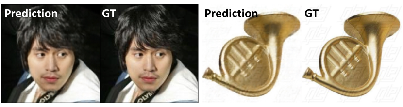
Qualitative results. Fig. 3 showcases G-NPF’s ability to recover high-frequency details in image regression, producing reconstructions that closely match the ground truth with high fidelity. This highlights the effectiveness of our approach. Additional qualitative results, including image completion, are provided in Appendix E.1. Specifically, Fig. 7 in the Appendix demonstrates that G-NPF can reconstruct full signals from minimal observations, further validating its capability.
4.2 G-NPF in 3D novel view synthesis
We continue with experiments in 3D novel view synthesis, a canonical task to evaluate 3D Neural Radiance Fields. We follow the implementation of (Guo et al., 2023; Chen & Wang, 2022). Briefly, our input context set comprises camera rays and their corresponding image pixels from one or two views. These are split into 256 tokens, each projected into a 512D vector via a linear layer and self-attention. Two MLPs predict 256 geometric bases: one generates 3D Gaussian parameters, and the other outputs 32D latent representations. From these, we derive object- and ray-specific modulating vectors (both 512D). Our NeRF function includes four layers—two modulated and two shared—with further details in Appendix C.1.
| Method | Views | Car | Lamps | Chairs |
|---|---|---|---|---|
| Learn Init | 25 | 22.80 | 22.35 | 18.85 |
| Tran-INR | 1 | 23.78 | 22.76 | 19.66 |
| NeRF-VAE | 1 | 21.79 | 21.58 | 17.15 |
| PONP | 1 | 24.17 | 22.78 | 19.48 |
| VNP | 1 | 24.21 | 24.10 | 19.54 |
| G-NPF (Ours) | 1 | 25.13 | 24.59 | 20.74 |
| Tran-INR | 2 | 25.45 | 23.11 | 21.13 |
| PONP | 2 | 25.98 | 23.28 | 19.48 |
| G-NPF (Ours) | 2 | 26.39 | 25.32 | 22.68 |
ShapeNet (Chang et al., 2015).
We follow the data setup of (Tancik et al., 2021), with objects from three ShapeNet categories: chairs, cars, and lamps. For each 3D object, 25 views of size images are generated from viewpoints randomly selected on a sphere. The objects in each category are divided into training and testing sets, with each training object consisting of 25 views with known camera poses. At test time, a random input view is sampled to evaluate the performance of the novel view synthesis. Following the setting of previous methods (Chen & Wang, 2022), we focus on the single-view (1-shot) and 2-view (2-shot) versions of the task, where one or two images with their corresponding camera rays are provided as the context.
We first compare with probabilistic Neural Field baselines, including NeRF-VAE (Kosiorek et al., 2021), PONP (Gu et al., 2023), and VNP (Guo et al., 2023). Like G-NPF, PONP (Gu et al., 2023) and VNP (Guo et al., 2023) also use Neural Processes, without, however, considering either geometric or hierarchical priors. Secondly, we also compare with well-established deterministic Neural Fields, including LearnInit (Tancik et al., 2021) and TransINR (Chen & Wang, 2022). We note that recent works (Liu et al., 2023; Shi et al., 2023b) have shown that training on massive 3D datasets (Deitke et al., 2023) is highly beneficial for Neural Radiance Fields. We leave massive-scale settings and comparisons to future work. Thirdly, to demonstrate the flexibility of G-NPF to handle complex scenes, we integrate with GNT (Wang et al., 2022) and conduct experiments on the NeRF Synthetic dataset (Mildenhall et al., 2021).
Quantitative results. We show Peak Signal-to-Noise Ratio (PSNR) results in Table 2. G-NPF consistently outperforms all other baselines across all categories by a significant margin. On average, G-NPF outperforms the probabilistic Neural Field baselines such as VNP (Guo et al., 2023), by 0.87 PSNR, indicating that adding structure in the form of geometric and hierarchical priors leads to better generalization. With two views for context, G-NPF improves significantly by about PSNR.
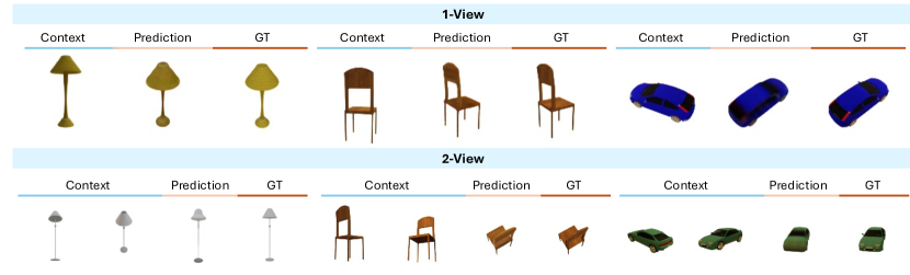
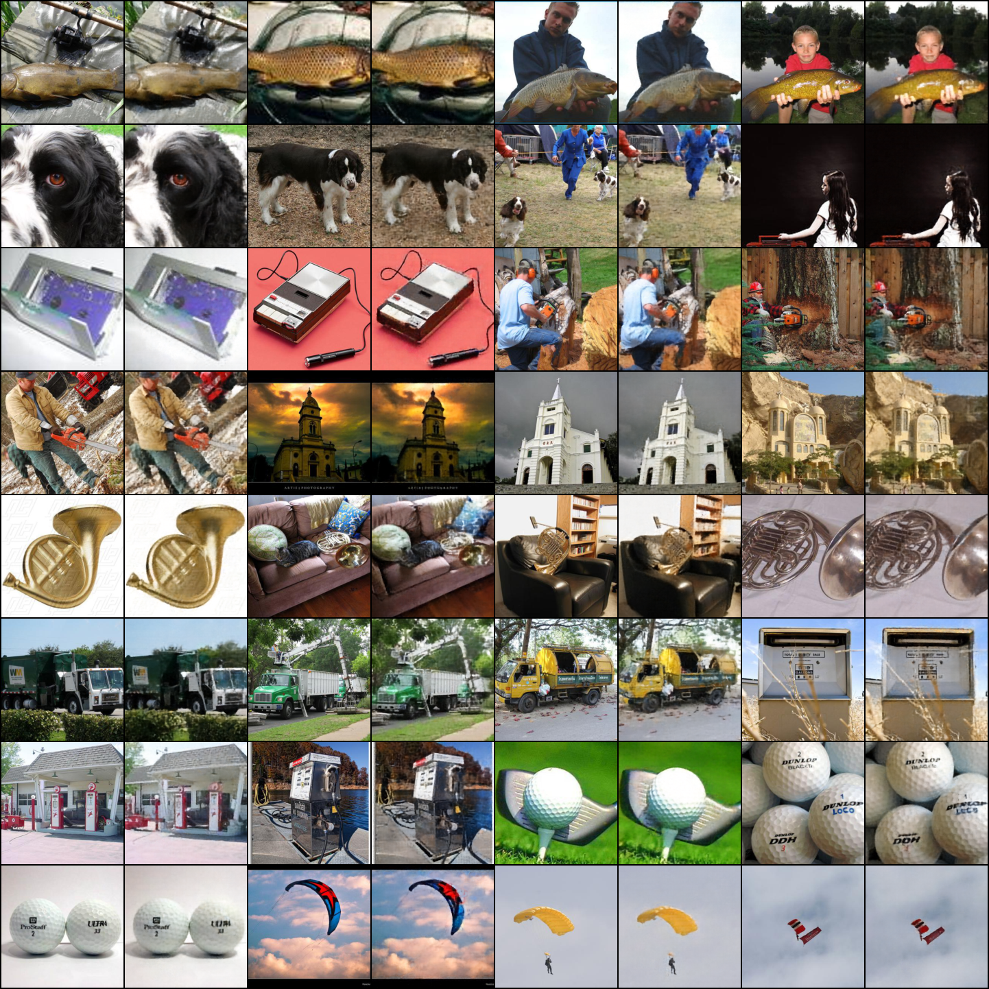
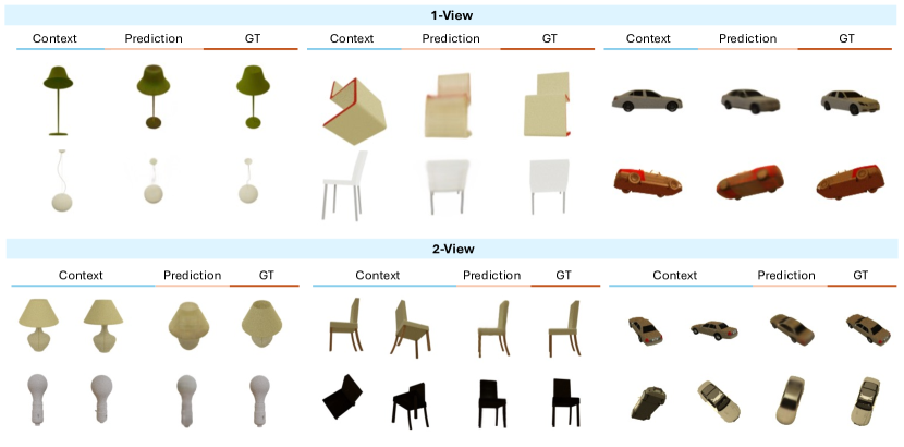
Qualitative results. In Fig. 4, we visualize the results on novel view synthesis of ShapeNet objects. G-NPF can infer object-specific radiance fields and render high-quality 2D images of the objects from novel camera views, even with only 1 or 2 views as context. More results and comparisons with other VNP are provided in Appendix E.
NeRF Synthetic (Mildenhall et al., 2021).
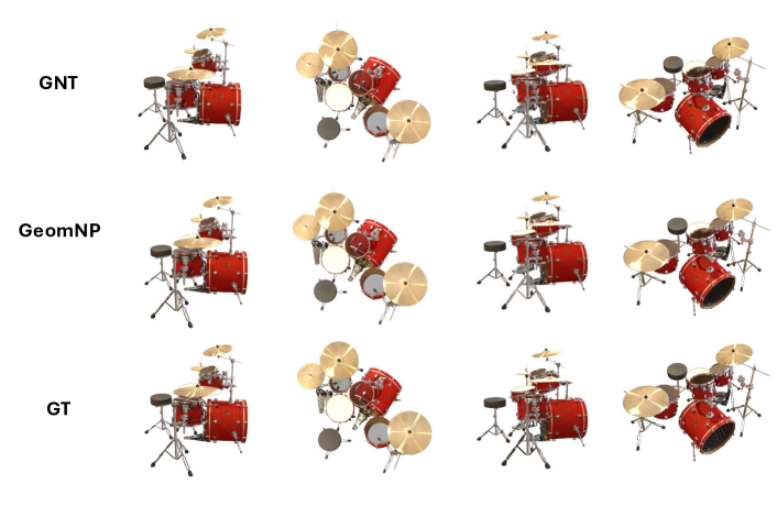
We further evaluate on the NeRF Synthetic dataset against recent state-of-the-art, including GNT (Wang et al., 2022), MatchNeRF (Chen et al., 2023a), and GeFu (Liu et al., 2024). For a fair comparison, we use the same encoder and NeRF network architecture while integrating our probabilistic framework into GNT. Following GeFu, we assess performance in 2-view and 3-view settings.
| Models | # Views | PSNR () | SSIM () | LPIPS () |
|---|---|---|---|---|
| GNT | 1 | 10.25 | 0.583 | 0.496 |
| G-NPF | 1 | 20.07 | 0.815 | 0.208 |
| GNT | 2 | 23.47 | 0.877 | 0.151 |
| MatchNeRF | 2 | 20.57 | 0.864 | 0.200 |
| GeFu | 2 | 25.30 | 0.939 | 0.082 |
| G-NPF | 2 | 25.66 | 0.926 | 0.081 |
| GNT | 3 | 25.80 | 0.905 | 0.104 |
| MatchNeRF | 3 | 23.20 | 0.897 | 0.164 |
| GeFu | 3 | 26.99 | 0.952 | 0.070 |
| G-NPF | 3 | 27.85 | 0.958 | 0.068 |
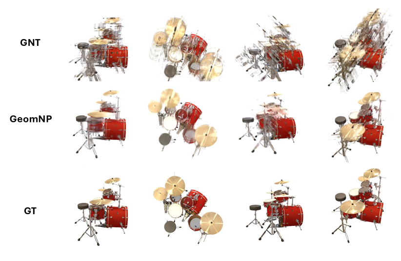
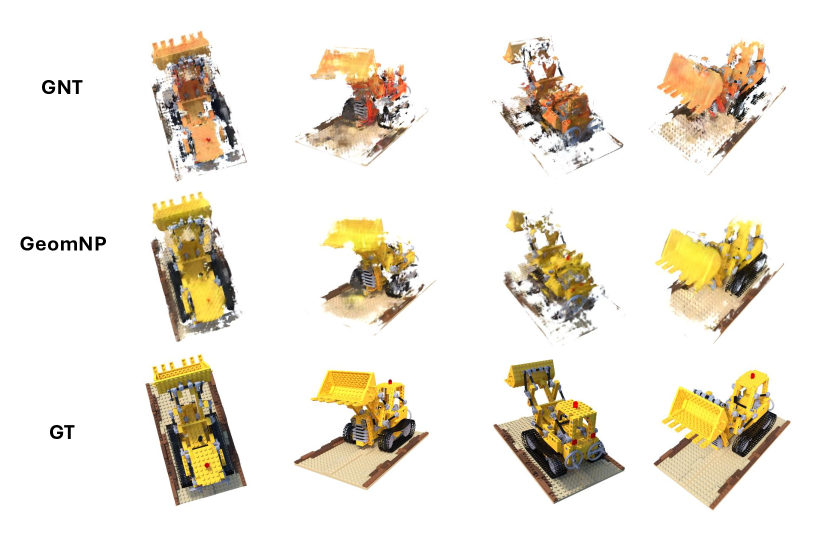
Quantitative results. We present results in Table 3. We observe that G-NPF surpasses GeFu by approximately 1 PSNR in the 3-view setting, validating the effectiveness of our probabilistic framework and geometric bases. Moreover, we consider a challenging 1-view setting to examine the model’s robustness under extremely limited context. Both Table 3 and Figure 8 indicate that G-NPF reconstructs novel views effectively also with only a single view for context, in contrast to GNT that fails in this setting. We furthermore test cross-category generalization for our model and GNT without retraining, training on the drums category and evaluating on lego. As shown in Figure 9, G-NPF leverages the available context information more effectively, producing higher-quality generations with better color fidelity compared to GNT. We give additional details in Appendix E.2.
4.3 G-NPF in 1D signal regression
Following the previous works’ implementation (Guo et al., 2023; Kim et al., 2019), we conduct 1D signal regression experiments using synthetic functions drawn from Gaussian processes (GPs) with RBF and Matern kernels. This kernel selection, as advocated by Kim et al. (2022), ensures diverse function characteristics spanning smoothness, periodicity, and local variability. To evaluate performance, we adopt two key metrics: (1) context reconstruction error, quantifying the log-likelihood of observed data points (context set), and (2) target prediction error, measuring the log-likelihood of extrapolated predictions (target set). We compare with three baselines, VNP (Guo et al., 2023), CNP (Garnelo et al., 2018a), and ANP (Kim et al., 2019).
Quantitative results. We present a quantitative comparison with baselines in Table 5. G-NPF consistently outperforms the baselines across two types of synthetic data, demonstrating its effectiveness and flexibility in different signals.
4.4 Ablations
| RBF kernel GP | Matern kernel GP | |||
|---|---|---|---|---|
| Method | Context | Target | Context | Target |
| CNP | ||||
| Stacked ANP | ||||
| VNP | ||||
| G-NPF | ||||
| PSNR () | |||
|---|---|---|---|
| ✗ | ✓ | ✓ | 23.06 |
| ✓ | ✗ | ✗ | 25.98 |
| ✓ | ✓ | ✗ | 26.24 |
| ✓ | ✗ | ✓ | 26.29 |
| ✓ | ✓ | ✓ | 26.48 |
| Image Regression | NeRF | ||||
| # Bases | 49 | 169 | 484 | 100 | 250 |
| PSNR () | 28.59 | 33.74 | 44.24 | 24.31 | 24.59 |
Geometric bases.
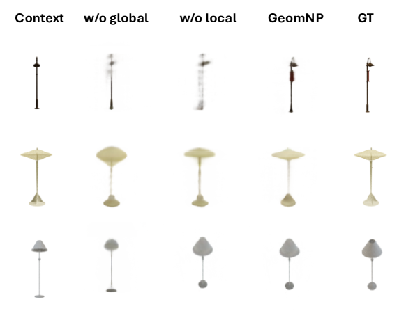
We first ablate the effectiveness of the proposed geometric bases on a subset of the 3D Lamps scene synthesis task. As shown in Table 5 (rows 1 and 5), with the geometric bases, GeomNP performs clearly better. This indicates the importance of the structure information modeled in the geometric bases. Moreover, the bases perform well without hierarchical latent variables, demonstrating their ability to construct 3D signals from limited 2D context.
We further analyze the sensitivity to the number of geometric bases in CelebA image regression and Lamps NeRF tasks. Results in Table 6 show that more bases lead to better accuracies and better generalization. We choose the number of bases by balancing the performance and computation.
Hierarchical latent variables.
We ablate the importance of the hierarchical nature of G-NPF on a subset of the Lamps dataset. The last four rows of Table 5 show that both global and local latent variables contribute to improved accuracy, with their combination yielding the best performance. Furthermore, the qualitative ablation study on hierarchical latent variables in Fig. 13 in the Appendix E.5 confirms that they effectively capture global and local structures, respectively.
5 Related Work
Neural Fields (NeFs) and Generalization. Neural Fields (NeFs) map coordinates to signals, providing a compact and flexible continuous data representation (Sitzmann et al., 2020b; Tancik et al., 2020). They are widely used for 3D object and scene modeling (Chen & Zhang, 2019; Park et al., 2019; Mescheder et al., 2019; Genova et al., 2020; Niemeyer & Geiger, 2021). However, how to generalize to new scenes without retraining remains a problem. Many previous methods attempt to use meta-learning to achieve NeF generalization. Specifically, gradient-based meta-learning algorithms such as Model-Agnostic Meta Learning (MAML) (Finn et al., 2017) and Reptile (Nichol et al., 2018) have been used to adapt NeFs to unseen data samples in a few gradient steps (Lee et al., 2021; Sitzmann et al., 2020a; Tancik et al., 2021). Another line of work uses HyperNet (Ha et al., 2016) to predict modulation vectors for each data instance, scaling and shifting the activations in all layers of the shared MLP (Mehta et al., 2021; Dupont et al., 2022a, b). Some methods use HyperNet to predict the weight matrix of NeF functions (Dupont et al., 2021; Zhang et al., 2023). Transformers (Vaswani et al., 2017) have also been used as hypernetworks to predict column vectors in the weight matrix of MLP layers (Chen & Wang, 2022; Dupont et al., 2022b). In addition, (Reizenstein et al., 2021; Wang et al., 2022) use transformers specifically for NeRF. Such methods are deterministic and do not consider the uncertainty of a scene when only partially observed. Other approaches model NeRF from a probabilistic perspective (Kosiorek et al., 2021; Hoffman et al., 2023; Dupont et al., 2021; Moreno et al., 2023; Erkoç et al., 2023). For instance, NeRF-VAE (Kosiorek et al., 2021) learns a distribution over radiance fields using latent scene representations based on VAE (Kingma & Welling, 2013) with amortized inference. Normalizing flow (Winkler et al., 2019) has also been used with variational inference to quantify uncertainty in NeRF representations (Shen et al., 2022; Wei et al., 2023). However, these methods do not consider potential structural information, such as the geometric characteristics of signals, which our approach explicitly models.
Neural Processes. Neural Processes (NPs) (Garnelo et al., 2018b) is a meta-learning framework that characterizes distributions over functions, enabling probabilistic inference, rapid adaptation to novel observations, and the capability to estimate uncertainties. This framework is divided into two classes of research. The first one concentrates on the marginal distribution of latent variables (Garnelo et al., 2018b), whereas the second targets the conditional distributions of functions given a set of observations (Garnelo et al., 2018a; Gordon et al., 2019). Typically, MLP is employed in Neural Processes methods. To improve this, Attentive Neural Processes (ANP) (Kim et al., 2019) integrate the attention mechanism to improve the representation of individual context points. Similarly, Transformer Neural Processes (TNP) (Nguyen & Grover, 2022) view each context point as a token and utilize transformer architecture to effectively approximate functions. Additionally, the Versatile Neural Process (VNP) (Guo et al., 2023) employs attentive neural processes for neural field generalization but does not consider the information misalignment between the 2D context set and the 3D target points. The hierarchical structure in VNP is more sequential than global-to-local. Conversely, PONP (Gu et al., 2023) is agnostic to neural-field specifics and concentrates on the neural process perspective. In this work, we consider a hierarchical neural process to model the structure information of the scene.
6 Conclusion
In this paper, we addressed the challenge of Neural Field (NeF) generalization, enabling models to rapidly adapt to new signals with limited observations. To achieve this, we proposed Geometric Neural Processes (G-NPF), a probabilistic neural radiance field that explicitly captures uncertainty. By formulating neural field generalization in a probabilistic framework, G-NPF incorporates uncertainty and infers NeF function distributions directly from sparse context images. To embed structural priors, we introduce geometric bases, which learn to provide structured spatial information. Additionally, our hierarchical neural process modeling leverages both global and local latent variables to parameterize NeFs effectively. In practice, G-NPF extends to 1D, 2D, and 3D signal generalization, demonstrating its versatility across different modalities.
Impact Statement
This paper contributes to the advancement of Machine Learning. While our work may have various societal implications, none require specific emphasis at this stage.
References
- Arandjelović & Zisserman (2021) Arandjelović, R. and Zisserman, A. Nerf in detail: Learning to sample for view synthesis. arXiv preprint arXiv:2106.05264, 2021.
- Barron et al. (2021) Barron, J. T., Mildenhall, B., Tancik, M., Hedman, P., Martin-Brualla, R., and Srinivasan, P. P. Mip-nerf: A multiscale representation for anti-aliasing neural radiance fields. In Proceedings of the IEEE/CVF International Conference on Computer Vision, pp. 5855–5864, 2021.
- Bruinsma et al. (2023) Bruinsma, W. P., Markou, S., Requiema, J., Foong, A. Y., Andersson, T. R., Vaughan, A., Buonomo, A., Hosking, J. S., and Turner, R. E. Autoregressive conditional neural processes. arXiv preprint arXiv:2303.14468, 2023.
- Chang et al. (2015) Chang, A. X., Funkhouser, T., Guibas, L., Hanrahan, P., Huang, Q., Li, Z., Savarese, S., Savva, M., Song, S., Su, H., et al. Shapenet: An information-rich 3d model repository. arXiv preprint arXiv:1512.03012, 2015.
- Charatan et al. (2024) Charatan, D., Li, S. L., Tagliasacchi, A., and Sitzmann, V. pixelsplat: 3d gaussian splats from image pairs for scalable generalizable 3d reconstruction. In Proceedings of the IEEE/CVF Conference on Computer Vision and Pattern Recognition, pp. 19457–19467, 2024.
- Chen et al. (2022) Chen, A., Xu, Z., Geiger, A., Yu, J., and Su, H. Tensorf: Tensorial radiance fields. In European Conference on Computer Vision, pp. 333–350. Springer, 2022.
- Chen & Wang (2022) Chen, Y. and Wang, X. Transformers as meta-learners for implicit neural representations. In European Conference on Computer Vision, pp. 170–187. Springer, 2022.
- Chen et al. (2023a) Chen, Y., Xu, H., Wu, Q., Zheng, C., Cham, T.-J., and Cai, J. Explicit correspondence matching for generalizable neural radiance fields. arXiv preprint arXiv:2304.12294, 2023a.
- Chen et al. (2025) Chen, Y., Xu, H., Zheng, C., Zhuang, B., Pollefeys, M., Geiger, A., Cham, T.-J., and Cai, J. Mvsplat: Efficient 3d gaussian splatting from sparse multi-view images. In European Conference on Computer Vision, pp. 370–386. Springer, 2025.
- Chen & Zhang (2019) Chen, Z. and Zhang, H. Learning implicit fields for generative shape modeling. In Proceedings of the IEEE/CVF conference on computer vision and pattern recognition, pp. 5939–5948, 2019.
- Chen et al. (2023b) Chen, Z., Li, Z., Song, L., Chen, L., Yu, J., Yuan, J., and Xu, Y. Neurbf: A neural fields representation with adaptive radial basis functions. In Proceedings of the IEEE/CVF International Conference on Computer Vision, pp. 4182–4194, 2023b.
- de Vries et al. (2023) de Vries, L., van Herten, R. L., Hoving, J. W., Išgum, I., Emmer, B. J., Majoie, C. B., Marquering, H. A., and Gavves, E. Spatio-temporal physics-informed learning: A novel approach to ct perfusion analysis in acute ischemic stroke. Medical image analysis, 90:102971, 2023.
- Deitke et al. (2023) Deitke, M., Schwenk, D., Salvador, J., Weihs, L., Michel, O., VanderBilt, E., Schmidt, L., Ehsani, K., Kembhavi, A., and Farhadi, A. Objaverse: A universe of annotated 3d objects. In Proceedings of the IEEE/CVF Conference on Computer Vision and Pattern Recognition, pp. 13142–13153, 2023.
- Deng et al. (2009) Deng, J., Dong, W., Socher, R., Li, L.-J., Li, K., and Fei-Fei, L. Imagenet: A large-scale hierarchical image database. In 2009 IEEE conference on computer vision and pattern recognition, pp. 248–255. Ieee, 2009.
- Dupont et al. (2021) Dupont, E., Teh, Y. W., and Doucet, A. Generative models as distributions of functions. arXiv preprint arXiv:2102.04776, 2021.
- Dupont et al. (2022a) Dupont, E., Kim, H., Eslami, S., Rezende, D., and Rosenbaum, D. From data to functa: Your data point is a function and you can treat it like one. arXiv preprint arXiv:2201.12204, 2022a.
- Dupont et al. (2022b) Dupont, E., Loya, H., Alizadeh, M., Goliński, A., Teh, Y. W., and Doucet, A. Coin++: Neural compression across modalities. arXiv preprint arXiv:2201.12904, 2022b.
- Erkoç et al. (2023) Erkoç, Z., Ma, F., Shan, Q., Nießner, M., and Dai, A. Hyperdiffusion: Generating implicit neural fields with weight-space diffusion. In Proceedings of the IEEE/CVF International Conference on Computer Vision, pp. 14300–14310, 2023.
- Finn et al. (2017) Finn, C., Abbeel, P., and Levine, S. Model-agnostic meta-learning for fast adaptation of deep networks. In International conference on machine learning, pp. 1126–1135. PMLR, 2017.
- Garnelo et al. (2018a) Garnelo, M., Rosenbaum, D., Maddison, C., Ramalho, T., Saxton, D., Shanahan, M., Teh, Y. W., Rezende, D., and Eslami, S. A. Conditional neural processes. In International conference on machine learning, pp. 1704–1713. PMLR, 2018a.
- Garnelo et al. (2018b) Garnelo, M., Schwarz, J., Rosenbaum, D., Viola, F., Rezende, D. J., Eslami, S., and Teh, Y. W. Neural processes. arXiv preprint arXiv:1807.01622, 2018b.
- Genova et al. (2020) Genova, K., Cole, F., Sud, A., Sarna, A., and Funkhouser, T. Local deep implicit functions for 3d shape. In Proceedings of the IEEE/CVF conference on computer vision and pattern recognition, pp. 4857–4866, 2020.
- Gordon et al. (2019) Gordon, J., Bruinsma, W. P., Foong, A. Y., Requeima, J., Dubois, Y., and Turner, R. E. Convolutional conditional neural processes. arXiv preprint arXiv:1910.13556, 2019.
- Gu et al. (2023) Gu, J., Wang, K.-C., and Yeung, S. Generalizable neural fields as partially observed neural processes. In Proceedings of the IEEE/CVF International Conference on Computer Vision, pp. 5330–5339, 2023.
- Guo et al. (2023) Guo, Z., Lan, C., Zhang, Z., Lu, Y., and Chen, Z. Versatile neural processes for learning implicit neural representations. arXiv preprint arXiv:2301.08883, 2023.
- Ha et al. (2016) Ha, D., Dai, A. M., and Le, Q. V. Hypernetworks. ArXiv, abs/1609.09106, 2016. URL https://api.semanticscholar.org/CorpusID:208981547.
- Hoffman et al. (2023) Hoffman, M. D., Le, T. A., Sountsov, P., Suter, C., Lee, B., Mansinghka, V. K., and Saurous, R. A. Probnerf: Uncertainty-aware inference of 3d shapes from 2d images. In International Conference on Artificial Intelligence and Statistics, pp. 10425–10444. PMLR, 2023.
- Hong et al. (2023) Hong, Y., Zhang, K., Gu, J., Bi, S., Zhou, Y., Liu, D., Liu, F., Sunkavalli, K., Bui, T., and Tan, H. Lrm: Large reconstruction model for single image to 3d. arXiv preprint arXiv:2311.04400, 2023.
- Howard (2020) Howard, J. Imagenette. https://github.com/fastai/imagenette, 2020.
- Kajiya & Von Herzen (1984) Kajiya, J. T. and Von Herzen, B. P. Ray tracing volume densities. ACM SIGGRAPH computer graphics, 18(3):165–174, 1984.
- Karras et al. (2020) Karras, T., Laine, S., Aittala, M., Hellsten, J., Lehtinen, J., and Aila, T. Analyzing and improving the image quality of stylegan. In Proceedings of the IEEE/CVF conference on computer vision and pattern recognition, pp. 8110–8119, 2020.
- Kerbl et al. (2023) Kerbl, B., Kopanas, G., Leimkühler, T., and Drettakis, G. 3d gaussian splatting for real-time radiance field rendering. 2023.
- Kim et al. (2023) Kim, C., Lee, D., Kim, S., Cho, M., and Han, W.-S. Generalizable implicit neural representations via instance pattern composers. In Proceedings of the IEEE/CVF Conference on Computer Vision and Pattern Recognition, pp. 11808–11817, 2023.
- Kim et al. (2019) Kim, H., Mnih, A., Schwarz, J., Garnelo, M., Eslami, A., Rosenbaum, D., Vinyals, O., and Teh, Y. W. Attentive neural processes. arXiv preprint arXiv:1901.05761, 2019.
- Kim et al. (2022) Kim, M., Go, K., and Yun, S.-Y. Neural processes with stochastic attention: Paying more attention to the context dataset. arXiv preprint arXiv:2204.05449, 2022.
- Kingma & Welling (2013) Kingma, D. P. and Welling, M. Auto-encoding variational bayes. arXiv preprint arXiv:1312.6114, 2013.
- Kosiorek et al. (2021) Kosiorek, A. R., Strathmann, H., Zoran, D., Moreno, P., Schneider, R., Mokrá, S., and Rezende, D. J. Nerf-vae: A geometry aware 3d scene generative model. In International Conference on Machine Learning, pp. 5742–5752. PMLR, 2021.
- Lee et al. (2021) Lee, J., Tack, J., Lee, N., and Shin, J. Meta-learning sparse implicit neural representations. Advances in Neural Information Processing Systems, 34:11769–11780, 2021.
- Liu et al. (2023) Liu, R., Wu, R., Van Hoorick, B., Tokmakov, P., Zakharov, S., and Vondrick, C. Zero-1-to-3: Zero-shot one image to 3d object. In Proceedings of the IEEE/CVF international conference on computer vision, pp. 9298–9309, 2023.
- Liu et al. (2024) Liu, T., Ye, X., Shi, M., Huang, Z., Pan, Z., Peng, Z., and Cao, Z. Geometry-aware reconstruction and fusion-refined rendering for generalizable neural radiance fields. In Proceedings of the IEEE/CVF Conference on Computer Vision and Pattern Recognition, pp. 7654–7663, 2024.
- Liu et al. (2015) Liu, Z., Luo, P., Wang, X., and Tang, X. Deep learning face attributes in the wild. In Proceedings of the IEEE international conference on computer vision, pp. 3730–3738, 2015.
- Mehta et al. (2021) Mehta, I., Gharbi, M., Barnes, C., Shechtman, E., Ramamoorthi, R., and Chandraker, M. Modulated periodic activations for generalizable local functional representations. In Proceedings of the IEEE/CVF International Conference on Computer Vision, pp. 14214–14223, 2021.
- Mescheder et al. (2019) Mescheder, L., Oechsle, M., Niemeyer, M., Nowozin, S., and Geiger, A. Occupancy networks: Learning 3d reconstruction in function space. In Proceedings of the IEEE/CVF conference on computer vision and pattern recognition, pp. 4460–4470, 2019.
- Mildenhall et al. (2021) Mildenhall, B., Srinivasan, P. P., Tancik, M., Barron, J. T., Ramamoorthi, R., and Ng, R. Nerf: Representing scenes as neural radiance fields for view synthesis. Communications of the ACM, 65(1):99–106, 2021.
- Moreno et al. (2023) Moreno, P., Kosiorek, A. R., Strathmann, H., Zoran, D., Schneider, R. G., Winckler, B., Markeeva, L., Weber, T., and Rezende, D. J. Laser: Latent set representations for 3d generative modeling. arXiv preprint arXiv:2301.05747, 2023.
- Müller et al. (2023) Müller, N., Siddiqui, Y., Porzi, L., Bulo, S. R., Kontschieder, P., and Nießner, M. Diffrf: Rendering-guided 3d radiance field diffusion. In Proceedings of the IEEE/CVF Conference on Computer Vision and Pattern Recognition, pp. 4328–4338, 2023.
- Müller et al. (2022) Müller, T., Evans, A., Schied, C., and Keller, A. Instant neural graphics primitives with a multiresolution hash encoding. ACM transactions on graphics (TOG), 41(4):1–15, 2022.
- Nguyen & Grover (2022) Nguyen, T. and Grover, A. Transformer neural processes: Uncertainty-aware meta learning via sequence modeling. arXiv preprint arXiv:2207.04179, 2022.
- Nichol et al. (2018) Nichol, A., Achiam, J., and Schulman, J. On first-order meta-learning algorithms. arXiv preprint arXiv:1803.02999, 2018.
- Niemeyer & Geiger (2021) Niemeyer, M. and Geiger, A. Giraffe: Representing scenes as compositional generative neural feature fields. In Proceedings of the IEEE/CVF Conference on Computer Vision and Pattern Recognition, pp. 11453–11464, 2021.
- Papa et al. (2024) Papa, S., Valperga, R., Knigge, D., Kofinas, M., Lippe, P., Sonke, J.-J., and Gavves, E. How to train neural field representations: A comprehensive study and benchmark. In Proceedings of the IEEE/CVF Conference on Computer Vision and Pattern Recognition, pp. 22616–22625, 2024.
- Park et al. (2019) Park, J. J., Florence, P., Straub, J., Newcombe, R., and Lovegrove, S. Deepsdf: Learning continuous signed distance functions for shape representation. In Proceedings of the IEEE/CVF conference on computer vision and pattern recognition, pp. 165–174, 2019.
- Raissi et al. (2019) Raissi, M., Perdikaris, P., and Karniadakis, G. E. Physics-informed neural networks: A deep learning framework for solving forward and inverse problems involving nonlinear partial differential equations. Journal of Computational physics, 378:686–707, 2019.
- Rasmussen (2003) Rasmussen, C. E. Gaussian processes in machine learning. In Summer school on machine learning, pp. 63–71. Springer, 2003.
- Reizenstein et al. (2021) Reizenstein, J., Shapovalov, R., Henzler, P., Sbordone, L., Labatut, P., and Novotny, D. Common objects in 3d: Large-scale learning and evaluation of real-life 3d category reconstruction. In Proceedings of the IEEE/CVF international conference on computer vision, pp. 10901–10911, 2021.
- Shen et al. (2022) Shen, J., Agudo, A., Moreno-Noguer, F., and Ruiz, A. Conditional-flow nerf: Accurate 3d modelling with reliable uncertainty quantification. In European Conference on Computer Vision, pp. 540–557. Springer, 2022.
- Shi et al. (2023a) Shi, R., Chen, H., Zhang, Z., Liu, M., Xu, C., Wei, X., Chen, L., Zeng, C., and Su, H. Zero123++: a single image to consistent multi-view diffusion base model. arXiv preprint arXiv:2310.15110, 2023a.
- Shi et al. (2023b) Shi, R., Chen, H., Zhang, Z., Liu, M., Xu, C., Wei, X., Chen, L., Zeng, C., and Su, H. Zero123++: a single image to consistent multi-view diffusion base model, 2023b.
- Shi et al. (2023c) Shi, Y., Wang, P., Ye, J., Long, M., Li, K., and Yang, X. Mvdream: Multi-view diffusion for 3d generation. arXiv preprint arXiv:2308.16512, 2023c.
- Sitzmann et al. (2020a) Sitzmann, V., Chan, E., Tucker, R., Snavely, N., and Wetzstein, G. Metasdf: Meta-learning signed distance functions. Advances in Neural Information Processing Systems, 33:10136–10147, 2020a.
- Sitzmann et al. (2020b) Sitzmann, V., Martel, J., Bergman, A., Lindell, D., and Wetzstein, G. Implicit neural representations with periodic activation functions. Advances in neural information processing systems, 33:7462–7473, 2020b.
- Suhail et al. (2022) Suhail, M., Esteves, C., Sigal, L., and Makadia, A. Generalizable patch-based neural rendering. In European Conference on Computer Vision, pp. 156–174. Springer, 2022.
- Szymanowicz et al. (2024) Szymanowicz, S., Rupprecht, C., and Vedaldi, A. Splatter image: Ultra-fast single-view 3d reconstruction. In Proceedings of the IEEE/CVF Conference on Computer Vision and Pattern Recognition, pp. 10208–10217, 2024.
- Tancik et al. (2020) Tancik, M., Srinivasan, P., Mildenhall, B., Fridovich-Keil, S., Raghavan, N., Singhal, U., Ramamoorthi, R., Barron, J., and Ng, R. Fourier features let networks learn high frequency functions in low dimensional domains. Advances in neural information processing systems, 33:7537–7547, 2020.
- Tancik et al. (2021) Tancik, M., Mildenhall, B., Wang, T., Schmidt, D., Srinivasan, P. P., Barron, J. T., and Ng, R. Learned initializations for optimizing coordinate-based neural representations. In Proceedings of the IEEE/CVF Conference on Computer Vision and Pattern Recognition, pp. 2846–2855, 2021.
- Tewari et al. (2023) Tewari, A., Yin, T., Cazenavette, G., Rezchikov, S., Tenenbaum, J., Durand, F., Freeman, B., and Sitzmann, V. Diffusion with forward models: Solving stochastic inverse problems without direct supervision. Advances in Neural Information Processing Systems, 36:12349–12362, 2023.
- Vaswani et al. (2017) Vaswani, A., Shazeer, N., Parmar, N., Uszkoreit, J., Jones, L., Gomez, A. N., Kaiser, Ł., and Polosukhin, I. Attention is all you need. Advances in neural information processing systems, 30, 2017.
- Wang et al. (2024) Wang, J., Zhang, Z., and Xu, R. Learning robust generalizable radiance field with visibility and feature augmented point representation. arXiv preprint arXiv:2401.14354, 2024.
- Wang et al. (2022) Wang, P., Chen, X., Chen, T., Venugopalan, S., Wang, Z., et al. Is attention all that nerf needs? arXiv preprint arXiv:2207.13298, 2022.
- Wang & Van Hoof (2020) Wang, Q. and Van Hoof, H. Doubly stochastic variational inference for neural processes with hierarchical latent variables. In International Conference on Machine Learning, pp. 10018–10028. PMLR, 2020.
- Wei et al. (2023) Wei, S., Zhang, J., Wang, Y., Xiang, F., Su, H., and Wang, H. Fg-nerf: Flow-gan based probabilistic neural radiance field for independence-assumption-free uncertainty estimation. arXiv preprint arXiv:2309.16364, 2023.
- Winkler et al. (2019) Winkler, C., Worrall, D. E., Hoogeboom, E., and Welling, M. Learning likelihoods with conditional normalizing flows. 2019.
- Xu et al. (2022) Xu, Q., Xu, Z., Philip, J., Bi, S., Shu, Z., Sunkavalli, K., and Neumann, U. Point-nerf: Point-based neural radiance fields. In Proceedings of the IEEE/CVF conference on computer vision and pattern recognition, pp. 5438–5448, 2022.
- Yin et al. (2022) Yin, Y., Kirchmeyer, M., Franceschi, J.-Y., Rakotomamonjy, A., and Gallinari, P. Continuous pde dynamics forecasting with implicit neural representations. arXiv preprint arXiv:2209.14855, 2022.
- Zhang et al. (2023) Zhang, B., Tang, J., Niessner, M., and Wonka, P. 3dshape2vecset: A 3d shape representation for neural fields and generative diffusion models. ACM Transactions on Graphics (TOG), 42(4):1–16, 2023.
Appendix A Neural Radiance Field Rendering
In this section, we outline the rendering function of NeRF (Mildenhall et al., 2021). A 5D neural radiance field represents a scene by specifying the volume density and the directional radiance emitted at every point in space. NeRF calculates the color of any ray traversing the scene based on principles from classical volume rendering (Kajiya & Von Herzen, 1984). The volume density quantifies the differential likelihood of a ray terminating at an infinitesimal particle located at . The anticipated color of a camera ray , within the bounds and , is determined as follows:
| (10) |
Here, the function represents the accumulated transmittance along the ray from to , which is the probability that the ray travels from to without encountering any other particles. To render a view from our continuous neural radiance field, we need to compute this integral for a camera ray traced through each pixel of the desired virtual camera.
Appendix B Hierarchical ELBO Derivation
Recall the hierarchical predictive distribution:
| (11) |
and its factorized version across target points:
We introduce a hierarchical variational posterior:
where are target-derived bases (available only at training). We then write the log-likelihood as
| (12) | ||||
We first apply Jensen’s inequality w.r.t. . This yields:
| (13) | ||||
Inside the expectation over , we have
We again apply Jensen’s inequality, but now w.r.t. , factorizing over :
| (14) | ||||
Putting this back into Eq. (13), we arrive at the hierarchical ELBO:
| (15) | ||||
The first expectation over enforces global consistency and penalizes deviations from the prior . The second set of expectations over shapes local reconstruction quality (via the log-likelihood) and penalizes deviations from the local prior .
Hence, the final ELBO (Equation 15) combines these outer and inner regularization terms with the expected log-likelihood of the target data . This allows the model to learn coherent global structure as well as local (coordinate-specific) details in a principled way.
Appendix C Implementation Details
C.1 Gaussian Construction
Since 3D Gaussians represent a special case involving quaternion-based transformations, we use them here as an illustrative example for constructing geometric bases. However, the method remains consistent with the construction of 1D and 2D Gaussian geometric bases.
Geometric Bases with 3D Gaussians.
To impose geometric structure on the context variables, we encode the context set into a set of geometric bases:
| (16) |
Each basis is thus defined by a 3D Gaussian and an associated semantic embedding . The center and covariance capture location and shape, while represents additional learned properties (e.g., color or texture). In our implementation, .
Self-Attention Construction.
We use a self-attention module, denoted Att, to extract these Gaussian parameters from the context data. Concretely,
| (17) |
where each call to Att produces tokens of hidden dimension . An MLP then maps each token into a 10-dimensional vector encoding: (i) the 3D center , (ii) a 3D scaling vector , and (iii) a 4D quaternion that, together, define the rotation matrix . Following Kerbl et al. (2023), we obtain the covariance via
| (18) |
where is the scaling matrix and is derived from . A separate MLP outputs the -dimensional embedding . Consequently, each is a fully parameterized 3D Gaussian plus a semantic vector, allowing the model to represent rich geometric information inferred from the context set.
C.2 Hierarchical Latent Variables
At the object level, the distribution of the global latent variable is obtained by aggregating all location representations from . We assume that follows a standard Gaussian distribution, and we generate its mean and variance using MLPs. We then sample a global modulation vector, , from its prior distribution .
Similarly, as shown in Fig. 5, we aggregate information for each target coordinate using , which is then processed through a Transformer along with to predict the local latent variable for each target point. The mean and variance of are obtained via MLPs.
C.3 Modulation
We use modulation to The latent variables for modulating the MLP are represented as . Our approach to the modulated MLP layer follows the style modulation techniques described in (Karras et al., 2020; Guo et al., 2023). Specifically, we consider the weights of an MLP layer (or 1x1 convolution) as , where and are the input and output dimensions respectively, and is the element at the -th row and -th column of .
To generate the style vector , we pass the latent variable through two MLP layers. Each element of the style vector is then used to modulate the corresponding parameter in .
| (19) |
where and denote the original and modulated weights, respectively.
The modulated weights are normalized to preserve training stability,
| (20) |
Appendix D Implementation Details
We train all our models with PyTorch. Adam optimizer is used with a learning rate of . For NeRF-related experiments, we follow the baselines (Chen & Wang, 2022; Guo et al., 2023) to train the model for 1000 epochs. All experiments are conducted on four NVIDIA A5000 GPUs. For the hyper-parameters and , we simply set them as .
Model Complexity
The comparison of the number of parameters is presented in Table. 7. Our method, GeomNP, utilizes fewer parameters than the baseline, VNP, while achieving better performance on the ShapeNet Car dataset in terms of PSNR.
| Method | # Parameters | PSNR |
|---|---|---|
| VNP | 34.3M | 24.21 |
| GeomNP | 24.0M | 25.13 |
Appendix E More Experimental Results
E.1 Image Regression
We provide more image regression results to demonstrate the effectiveness of our method as shown in Fig. 6.
Image Completion.
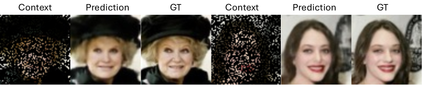
In addition, we also conduct experiments of G-NPF on image completion (also called image inpainting), which is a more challenging variant of image regression. Essentially, only part of the pixels are given as context, while the INR functions are required to complete the full image. Visualizations in Fig. 7 demonstrate the generalization ability of our method to recover realistic images with fine details based on very limited context ( pixels).
E.2 Comparison with GNT.
For fair comparison, we use GNT’s image encoder and predict the geometric bases, and GNT’s NeRF’ network for prediction. Fig. 8 shows that our method is effective when very limited context information is given, while GNT fails. This indicates that our method can sufficiently utilize the given information.
Cross-Category Example.
Additionally, we perform cross-category evaluation without retraining the model. The model is trained on drums category and evaluated on lego. As shown in Figure 9, G-NPF leverages the available context information more effectively, producing higher-quality generations with better color fidelity compared to GNT.
E.3 More results on ShapeNet
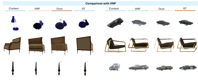
In this section, we demonstrate more experimental results on the novel view synthesis task on ShapeNet in Fig 10, comparison with VNP (Guo et al., 2023) in Fig. 11, and image regression on the Imagenette dataset in Fig. 6. The proposed method is able to generate realistic novel view synthesis and 2D images.
E.4 Training Time Comparison
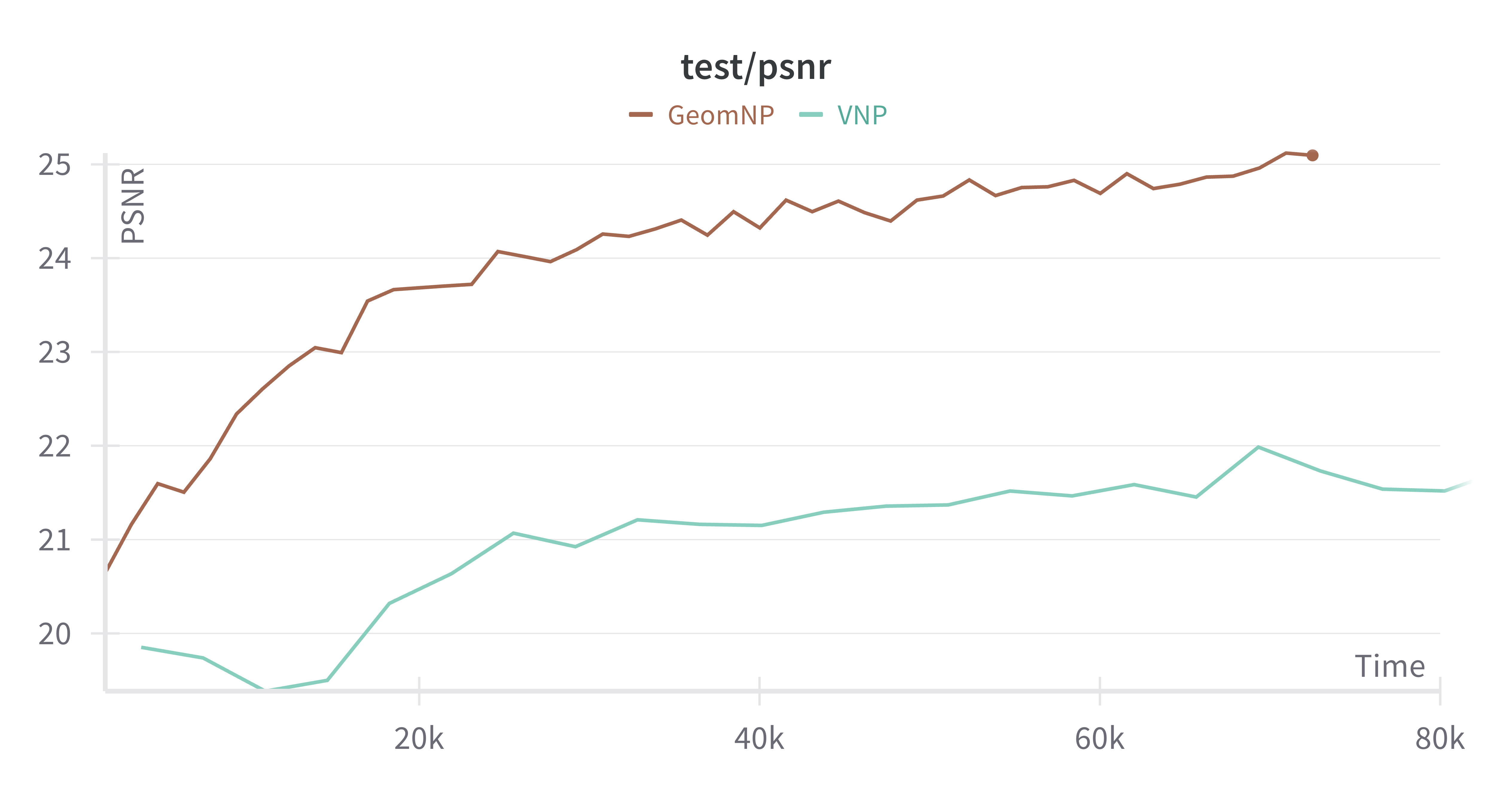
As illustrated in Fig.12, with the same training time, our method (GeomNP) demonstrates faster convergence and higher final PSNR compared to the baseline (VNP).
E.5 Qualitative ablation of the hierarchical latent variables
In this section, we perform a qualitative ablation study on the hierarchical latent variables. As illustrated in Fig. 13, the absence of the global variable prevents the model from accurately predicting the object’s outline, whereas the local variable captures fine-grained details. When both global and local variables are incorporated, GeomNP successfully estimates the novel view with high accuracy.
E.6 More multi-view reconstruction results
We integrate our method into GNT (Wang et al., 2022) framework and perform experiments on the Drums class of the NeRF synthetic dataset. Qualitative comparisons of multi-view results are presented in Fig. 14.
Appendix F Extending G-NPF to NeRFs
Notations. We denote 3D world coordinates by and a camera viewing direction by . Each point in 3D space have its color , which depends on the location and viewing direction . Points also have a density value that encodes opacity. We represent coordinates and view direction together as , color and density together as . When observing a 3D object from multiple locations, we denote all 3D points as and their colors and densities as . Assuming a ray starting from the camera origin and along direction , we sample points along the ray, with and corresponding colors and densities . Further, we denote the observations and as: the set of camera rays and the projected 2D pixels from the rays .
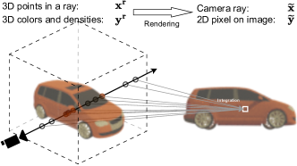
Background on Neural Radiance Fields. We formally describe Neural Radiance Field (NeRF) (Mildenhall et al., 2021; Arandjelović & Zisserman, 2021) as a continuous function , which maps 3D world coordinates and viewing directions to color and density values . That is, a NeRF function, , is a neural network-based function that represents the whole 3D object (e.g., a car in Fig. 15) as coordinates to color and density mappings. Learning a NeRF function of a 3D object is an inverse problem where we only have indirect observations of arbitrary 2D views of the 3D object, and we want to infer the entire 3D object’s geometry and appearance. With the NeRF function, given any camera pose, we can render a view on the corresponding 2D image plane by marching rays and using the corresponding colors and densities at the 3D points along the rays. Specifically, given a set of rays with view directions , we obtain a corresponding 2D image. The integration along each ray corresponds to a specific pixel on the 2D image using the volume rendering technique described in (Kajiya & Von Herzen, 1984), which is also illustrated in Fig. 15. Details about the integration are given in Appendix A.
F.1 Probabilistic NeRF Generalization
Deterministic Neural Radiance Fields
Probabilistic Neural Radiance Fields
As we are not just interested in fitting a single and specific 3D object but want to learn how to infer the Neural Radiance Field of any 3D object, we focus on probabilistic Neural Radiance Fields with the following factorization:
| (21) |
The generation process of this probabilistic formulation is as follows. We first start from (or sample) a set of rays . Conditioning on these rays, we sample 3D points in space . Then, we map these 3D points into their colors and density values with the NeRF function, . Last, we sample the 2D pixels of the viewing image that corresponds to the 3D ray with a probabilistic process. This corresponds to integrating colors and densities along the ray on locations .
The probabilistic model in Eq. 21 is for a single 3D object, thus requiring optimizing a function afresh for every new object, which is time-consuming. For NeRF generalization, we accelerate learning and improve generalization by amortizing the probabilistic model over multiple objects, obtaining per-object reconstructions by conditioning on context sets . For clarity, we use to indicate context sets with a few new observations for a new object, while indicates target sets containing 3D points or camera rays from novel views of the same object. Thus, we formulate a probabilistic NeRF for generalization as:
| (22) | ||||
As this paper focuses on generalization with new 3D objects, we keep the same sampling and integrating processes as in Eq. 21. We turn our attention to the modeling of the predictive distribution in the generalization step, which implies inferring the NeRF function.
Misalignment between 2D context and 3D structures
It is worth mentioning that the predictive distribution in 3D space is conditioned on 2D context pixels with their ray and 3D target points , which is challenging due to potential information misalignment. Thus, we need strong inductive biases with 3D structure information to ensure that 2D and 3D conditional information is fused reliably.
F.2 Geometric Bases
To mitigate the information misalignment between 2D context views and 3D target points, we introduce geometric bases , which induces prior structure to the context set geometrically. is the number of geometric bases.
Each geometric basis consists of a Gaussian distribution in the 3D point space and a semantic representation, i.e., , where and are the mean and covariance matrix of -th Gaussian in 3D space, and is its corresponding latent representation. Intuitively, the mixture of all 3D Gaussian distributions implies the structure of the object, while stores the corresponding semantic information. In practice, we use a transformer-based encoder to learn the Gaussian distributions and representations from the context sets, i.e., . Detailed architecture of the encoder is provided in Appendix C.1.
With the geometric bases , we review the predictive distribution from to . By inferring the function distribution , we reformulate the predictive distribution as:
| (23) |
where is the prior distribution of the NeRF function, and is the likelihood term. Note that the prior distribution of the NeRF function is conditioned on the target points and the geometric bases . Thus, the prior distribution is data-dependent on the target inputs, yielding a better generalization on novel target views of new objects. Moreover, since is constructed with continuous Gaussian distributions in the 3D space, the geometric bases can enrich the locality and semantic information of each discrete target point, enhancing the capture of high-frequency details (Chen et al., 2023b, 2022; Müller et al., 2022).
F.3 Geometric Neural Processes with Hierarchical Latent Variables
With the geometric bases, we propose Geometric Neural Processes (GeomNP) by inferring the NeRF function distribution in a probabilistic way. Based on the probabilistic NeRF generalization in Eq. 22, we introduce hierarchical latent variables to encode various spatial-specific information into , improving the generalization ability in different spatial levels. Since all rays are independent of each other, we decompose the predictive distribution in Eq. 23 as:
| (24) |
where the target input consists of location points for rays.
Further, we develop a hierarchical Bayes framework for GeomNP to accommodate the data structure of the target input in Eq. 24. We introduce an object-specific latent variable and individual ray-specific latent variables to represent the randomness of .
Within the hierarchical Bayes framework, encodes the entire object information from all target inputs and the geometric bases in the global level; while every encodes ray-specific information from in the local level, which is also conditioned on the global latent variable . The hierarchical architecture allows the model to exploit the structure information from the geometric bases in different levels, improving the model’s expressiveness ability. By introducing the hierarchical latent variables in Eq. 24, we model GeomNP as:
| (25) | ||||
where denotes the ray-specific likelihood term. In this term, we use the hierarchical latent variables to modulate a ray-specific NeRF function for prediction, as shown in Fig. 16. Hence, can explore global information of the entire object and local information of each specific ray, leading to better generalization ability on new scenes and new views. A graphical model of our method is provided in Fig. 17.
In the modeling of GeomNP, the prior distribution of each hierarchical latent variable is conditioned on the geometric bases and target input. We first represent each target location by integrating the geometric bases, i.e., , which aggregates the relevant locality and semantic information for the given input. Since contains Gaussians, we employ a Gaussian radial basis function in Eq. 26 between each target input and each geometric basis to aggregate the structural and semantic information to the 3D location representation. Thus, we obtain the 3D location representation as follows:
| (26) |
where is a learnable neural network. With the location representation , we next infer each latent variable hierarchically, in object and ray levels.
Object-specific Latent Variable. The distribution of the object-specific latent variable is obtained by aggregating all location representations:
| (27) |
where we assume is a standard Gaussian distribution and generate its mean and variance by a MLP. Thus, our model captures objective-specific uncertainty in the NeRF function.
Ray-specific Latent Variable. To generate the distribution of the ray-specific latent variable, we first average the location representations ray-wisely. We then obtain the ray-specific latent variable by aggregating the averaged location representation and the object latent variable through a lightweight transformer. We formulate the inference of the ray-specific latent variable as:
| (28) |
where is a sample from the prior distribution . Similar to the object-specific latent variable, we also assume the distribution is a mean-field Gaussian distribution with the mean and variance . We provide more details of the latent variables in Appendix C.2.
NeRF Function Modulation. With the hierarchical latent variables , we modulate a neural network for a 3D object in both object-specific and ray-specific levels. Specifically, the modulation of each layer is achieved by scaling its weight matrix with a style vector (Guo et al., 2023). The object-specific latent variable and ray-specific latent variable are taken as style vectors of the low-level layers and high-level layers, respectively. The prediction distribution are finally obtained by passing each location representation through the modulated neural network for the NeRF function. More details are provided in Appendix C.3.
F.4 Empirical Objective
Evidence Lower Bound. To optimize the proposed GeomNP, we apply variational inference (Garnelo et al., 2018b) and derive the evidence lower bound (ELBO) as:
| (29) | ||||
where is the involved variational posterior for the hierarchical latent variables. is the geometric bases constructed from the target sets , which are only accessible during training. The variational posteriors are inferred from the target sets during training, which introduces more information on the object. The prior distributions are supervised by the variational posterior using Kullback–Leibler (KL) divergence, learning to model more object information with limited context data and generalize to new scenes. Detailed derivations are provided in Appendix F.5.
For the geometric bases , we regularize the spatial shape of the context geometric bases to be closer to that of the target one by introducing a KL divergence. Therefore, given the above ELBO, our objective function consists of three parts: a reconstruction loss (MSE loss), KL divergences for hierarchical latent variables, and a KL divergence for the geometric bases. The empirical objective for the proposed GeomNP is formulated as:
| (30) | ||||
where is the prediction. and are hyperparameters to balance the three parts of the objective. The KL divergence on is to align the spatial location and the shape of two sets of bases.
F.5 Derivation of Evidence Lower Bound
Evidence Lower Bound. We optimize the model via variational inference (Garnelo et al., 2018b), deriving the evidence lower bound (ELBO):
| (31) | ||||
where the variational posterior factorizes as . Here, denotes geometric bases constructed from target data (available only during training). The KL terms regularize the hierarchical priors and to align with variational posteriors inferred from , enhancing generalization to context-only settings.
The propose GeomNP is formulated as:
| (32) |
where and denote prior distributions of a object-specific and each ray-specific latent variables, respectively. Then, the evidence lower bound is derived as follows.
| (33) | ||||
where is the variational posterior of the hierarchical latent variables.
Appendix G More Related Work
Generalizable Neural Radiance Fields (NeRF)
Advancements in neural radiance fields have focused on improving generalization across diverse scenes and objects. (Wang et al., 2022) propose an attention-based NeRF architecture, demonstrating enhanced capabilities in capturing complex scene geometries by focusing on informative regions. (Suhail et al., 2022) introduce a generalizable patch-based neural rendering approach, enabling models to adapt to new scenes without retraining. (Xu et al., 2022) present Point-NeRF, leveraging point-based representations for efficient scene modeling and scalability. (Wang et al., 2024) further enhance point-based methods by incorporating visibility and feature augmentation to improve robustness and generalization. (Liu et al., 2024) propose a geometry-aware reconstruction with fusion-refined rendering for generalizable NeRFs, improving geometric consistency and visual fidelity. Recently, the Large Reconstruction Model (LRM) (Hong et al., 2023) has drawn attention. It aims for single-image to 3D reconstruction, emphasizing scalability and handling of large datasets.
Gaussian Splatting-based Methods
Gaussian splatting (Kerbl et al., 2023) has emerged as an effective technique for efficient 3D reconstruction from sparse views. (Szymanowicz et al., 2024) propose Splatter Image for ultra-fast single-view 3D reconstruction. (Charatan et al., 2024) introduce pixelsplat, utilizing 3D Gaussian splats from image pairs for scalable generalizable reconstruction. (Chen et al., 2025) present MVSplat, focusing on efficient Gaussian splatting from sparse multi-view images. Our approach can be a complementary module for these methods by introducing a probabilistic neural processing scheme to fully leverage the observation.
Diffusion-based 3D Reconstruction
Integrating diffusion models into 3D reconstruction has shown promise in handling uncertainty and generating high-quality results. (Müller et al., 2023) introduce DiffRF, a rendering-guided diffusion model for 3D radiance fields. (Tewari et al., 2023) explore solving stochastic inverse problems without direct supervision using diffusion with forward models. (Liu et al., 2023) propose Zero-1-to-3, a zero-shot method for generating 3D objects from a single image without training on 3D data, utilizing diffusion models. (Shi et al., 2023a) introduce Zero123++, generating consistent multi-view images from a single input image using diffusion-based techniques. (Shi et al., 2023c) present MVDream, which uses multi-view diffusion for 3D generation, enhancing the consistency and quality of reconstructed models.