Coreset-Based Task Selection for Sample-Efficient
Meta-Reinforcement Learning

Abstract

We study task selection to enhance sample efficiency in model-agnostic meta-reinforcement learning (MAML-RL). Traditional meta-RL typically assumes that all available tasks are equally important, which can lead to task redundancy when they share significant similarities. To address this, we propose a coreset-based task selection approach that selects a weighted subset of tasks based on how diverse they are in gradient space, prioritizing the most informative and diverse tasks. Such task selection reduces the number of samples needed to find an $\epsilon$-close stationary solution by a factor of $\mathcal{O}(1/\epsilon)$. Consequently, it guarantees a faster adaptation to unseen tasks while focusing training on the most relevant tasks. As a case study, we incorporate task selection to MAML-LQR (Toso et al., 2024b), and prove a sample complexity reduction proportional to $\mathcal{O}(\log(1/\epsilon))$ when the task-specific cost also satisfy gradient dominance. Our theoretical guarantees underscore task selection as a key component for scalable and sample-efficient meta-RL. We numerically validate this trend across multiple RL benchmark problems, illustrating the benefits of task selection beyond the LQR baseline.

1 Introduction

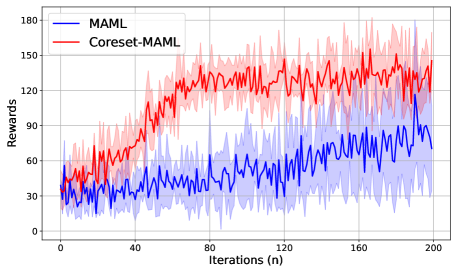
Figure 1: Comparison of coreset MAML-RL (this work) and MAML-RL on the hopper Mujoco environment (see appendix for details).

Meta-reinforcement learning (meta-RL) has emerged as a powerful framework for learning policies that can quickly adapt to unseen environments (Wang et al., 2016; Finn et al., 2017). In particular, the model-agnostic meta-reinforcement learning (MAML-RL) algorithm has demonstrated success in enabling agents to learn a shared policy initialization that is only a few policy gradient steps away from optimality for any seen and unseen task (Duan et al., 2016; Nagabandi et al., 2018). Such quick adaptation is crucial, for example, in robotics (Song et al., 2020), where agents often need to operate in dynamic environments and accomplish a variety of goals.

MAML-RL and meta-reinforcement learning more generally, typically assumes that all training tasks are equally important. This assumption may lead to task redundancy and excessive sampling costs as it is likely not worth sampling from multiple similar tasks; instead collecting data from a single representative task would suffice.

“Task selection” can be thought of a pre-processing step in the meta-learning pipeline. It seeks to identify a representative subset of tasks that captures the diversity across all training tasks, and then uses this smaller “coreset” for training. In particular, “coreset learning” has been proposed for data-efficient training of machine learning models (Mirzasoleiman et al., 2020; Pooladzandi et al., 2022; Yang et al., 2023). Related work has also employed coreset selection to select clients in federated learning (Balakrishnan et al., 2022) and continual learning (Tiwari et al., 2022; Wang et al., 2022). For meta-learning, and in the context of classification, Zhan and Anderson (2024) propose a data-efficient and robust task selection algorithm (DERTS) that outperforms existing sampling-based techniques. In essence, DERTS frames coreset learning as submodular optimization, where the goal is to select a subset of tasks that minimizes the maximum normed difference across task-specific gradients.

In the work above, it is assumed that task-specific gradients can be directly computed. In meta-RL, such an assumption may be restrictive as the meta-gradient depends on unknown task and trajectory distributions, where the later is also conditioned on the current policy. As such, it is challenging to compute the gradient via automatic differentiation (Rothfuss et al., 2018). To circumvent this, one must resort to gradient approximation, that by itself introduces extra difficulties to the analysis of meta-RL with task selection. Specifically, errors arising from gradient estimation and the meta-training on the coreset need to be carefully accounted for.

Contributions: Towards addressing these points, we propose a coreset-based task selection algorithm (inspired by DERTS) for meta-RL. The main contributions of our approach are:

$\bullet$ Algorithmic: This is the first work to propose a derivative-free coreset-based task selection approach for MAML-RL (Algorithm 1), which also comes with strong convergence guarantees (Section 3). We derive an ergodic convergence rate for non-concave task-specific reward functions (Theorem 1) and prove that Algorithm 1 finds an $\epsilon$-close stationary solution after $N=\mathcal{O}(1/\epsilon)$ iterations when the task selection bias is made sufficiently small. We also incorporate task selection to meta-learning for control via the MAML-LQR algorithm (Toso et al., 2024b) and show that it learns a provably fast-to-adapt LQR controller (Theorem 2) within $N=\mathcal{O}(\log(1/\epsilon))$ iterations while reducing task redundancy.

$\bullet$ Sample Complexity: We demonstrate that selecting a weighted subset of the most informative tasks reduces the sample complexity for achieving local convergence by a factor of ${\color[rgb]{0,0,1}\mathcal{O}(1/\epsilon)}$ (c.f. Section 4, Figure 1, and Corollary 1). In particular, this reduction is guaranteed when the set of training tasks is sufficiently large and tasks therein are sufficiently similar. Moreover, Algorithm 1 offers a sample complexity reduction proportional to $\mathcal{O}(\log(1/\epsilon))$ in the MAML-LQR setting (Corollary 2).

Related Work: Meta-reinforcement learning has been extensively studied across several applications, including robot manipulation (Yu et al., 2017), locomotion (Song et al., 2020), and building energy control (Luna Gutierrez and Leonetti, 2020). Most relevant to our work is Song et al. (2019, 2020), which is derivative-free but treats all tasks equally, leading to task redundancy. Task weighting is addressed in Shin et al. (2023) and Zhan and Anderson (2024) by selecting representative task subsets. However, Zhan and Anderson (2024) focuses on classification tasks and simplifies gradient approximation by using the model pre-activation outputs, while Shin et al. (2023) employs an information-theoretic metric for task selection and does not consider gradient-based training. Finally, in the context of control, the linear quadratic regulator (LQR) problem has become a key baseline for policy optimization in reinforcement learning. In particular, Molybog and Lavaei (2021); Musavi and Dullerud (2023); Toso et al. (2024b); Aravind et al. (2024); Pan and Zhu (2024) study the meta-LQR problem and provide guarantees for provably learning fast-to-adapt LQR controllers. Building on this, our work also integrates task selection into the MAML-LQR setting, demonstrating its effectiveness in reducing the sample complexity. A broader overview of related work is included in Section 6.1 of the appendix.

2 Preliminaries

We now introduce the MAML-RL problem (Finn et al., 2017) and formalize our coreset-based task selection that selects a weighted subset of tasks based on their diversity in gradient space.

2.1 Model Agnostic Meta-Reinforcement Learning

Let $T_{j}$ be a reinforcement learning task drawn from a task distribution $\mathcal{P}(\mathcal{T})$ over a set of tasks $\mathcal{T}$. Let $\mathcal{M}$ denote a set of $M$ tasks drawn from $\mathcal{P}(\mathcal{T})$, i.e., $\mathcal{M}:=\left\{T_{j}\mid j=1,2,\ldots,M\right\}$. The objective of MAML-RL is to learn a meta-policy $\pi_{\theta^{\star}}$ with meta-parameter $\theta^{\star}\in\Theta$, trained on $\mathcal{M}$, such that within a few policy gradient steps, $\pi_{\theta^{\star}}$ can be adapted to an unseen task-specific policy. We assume that all tasks share the same state and action spaces $\mathcal{S}$, and $\mathcal{A}$. In addition, each task $T_{j}$ is associated with a reward function $R_{j}$ and a transition distribution $q_{j}(s_{t+1}|s_{t},a_{t})$ at time step $t$. Also, let $J(\theta)$ and $J_{j}(\theta)$ be the MAML and task-specific reward functions, respectively. The one-shot MAML-RL problem is written as follows:

$$\theta^{\star}:=\text{argmax}_{\theta\in\Theta}~J(\theta):=\mathbb{E}_{T_{j}\sim\mathcal{P}(\mathcal{T})}J_{j}(\theta+\eta_{\text{inn}}\nabla J_{j}(\theta)),$$ (1)

for some positive inner step-size $\eta_{\text{inn}}$. Moreover, $J_{j}({\theta}):=\mathbb{E}_{{\tau}\sim\mathcal{P}_{T_{j}}({\tau}|{\theta})}\mathcal{R}_{j}({\tau})$ is the task-specific reward incurred by $\pi_{\theta}$, where $\mathcal{P}_{T_{j}}(\tau|\theta)$ is the distribution of trajectories $\tau$ conditioned on the policy $\pi_{\theta}$. We also define $\bar{\theta}:=\theta+\eta_{\text{inn}}\nabla_{\theta}J_{j}(\theta)$. Hence, the gradient-based MAML-RL update follows: $\theta\leftarrow\theta+\eta_{\text{out}}\nabla J(\theta)$ with $\eta_{\text{out}}$ denoting the outer step-size, and the MAML gradient given by

$$\nabla J(\theta)=\mathbb{E}_{T_{j}\sim\mathcal{P}(\mathcal{T})}\left[\mathbb{E}_{{\tau}\sim\mathcal{P}_{T_{j}}({\tau}|\bar{\theta})}(\nabla_{\bar{\theta}}\log\mathcal{P}_{T_{j}}({\tau}|\bar{\theta})R_{j}({\tau})\nabla\bar{\theta})\right],\text{ where}$$

$$\nabla_{\bar{\theta}}:=I+\eta_{\text{out}}\left(\int\mathcal{P}_{T_{j}}(\tau|\theta)\nabla^{2}\log\pi_{\theta}(\tau)R_{j}(\tau)+\mathcal{P}_{T_{j}}(\tau|\theta)\nabla_{\theta}\log\pi_{\theta}(\tau)\nabla_{\theta}\log\pi_{\theta}(\tau)^{\top}R_{j}(\tau)d\tau\right).$$

The direct computation of $J_{j}(\theta)$ and $\nabla J(\theta)$ may be intractable due to the expectation over unknown trajectory and task distributions. A standard approach to approximate $J_{j}(\theta)$ is to sample multiple trajectories $\tau_{l}$ by playing $\pi_{\theta}$ and then computing the empirical task-specific reward function $\hat{J}_{j}(\theta)$ (Liu et al., 2019; Rothfuss et al., 2018; Song et al., 2019). On the other hand, following Song et al. (2019, 2020), we propose a derivative-free method for estimating the task-specific and MAML gradients through querying/estimating task-specific rewards.

2.2 Task Selection

Motivated by Yang et al. (2023); Zhan and Anderson (2024), we argue that not all the tasks in the task pool $\mathcal{M}$ are equally important for meta-training. Since multiple tasks may share similarities, that may lead to task redundancy and sample inefficiency, as it requires collecting data from multiple similar tasks when, in principle, collecting data from a single task that is representative of all the similar tasks should suffice for training. Our goal is to select a subset of tasks, $\mathcal{S}$ (the coreset), from the task pool $\mathcal{M}$ that best represents the diversity of the tasks in $\mathcal{M}$, such that the performance of the model trained on a weighted subset of $\mathcal{S}$ is sufficiently close to that of a model trained on the full task pool $\mathcal{M}$. In particular, we will prove that by carefully controlling the task selection bias one may achieve a substantial sample complexity reduction in the meta-training.

The main steps of our meta training algorithm are: $(i)$ coreset selection—selecting the coreset $\mathcal{S}\subseteq\mathcal{M}$, $(ii)$ weight allocation for each task in $\mathcal{S}$ such that it captures the relative importance of the task, and $(iii)$ meta-training on the coreset $\mathcal{S}$ and its corresponding weighting. In the following subsections we introduce the concept of gradient approximation over the task pools and establish the selection criterion for assigning tasks in $\mathcal{M}$ to $\mathcal{S}$.

2.2.1 Full Gradient Approximation over the Task Pool

Our aim is to select the coreset $\mathcal{S}\subseteq\mathcal{M}$ with $\mathcal{S}:=\left\{T_{i}\mid i=\alpha_{1},\alpha_{2},\ldots,\alpha_{L}\right\}$, where $\alpha_{i}\in[M]$ and $L\leq M$, with corresponding weights $\left\{\gamma_{i}~|~i=1,2,\ldots,L\right\}$, such that the gradient for training on $\mathcal{S}$ with corresponding weights $\gamma_{i}$ approximates the meta-gradient on $\mathcal{M}$.

To better understand the coreset-based task selection we let $\Gamma:\mathcal{M}\rightarrow\mathcal{S}$ be a mapping from the task pool $\mathcal{M}$ to the coreset $\mathcal{S}$, i.e., that maps a task $T_{j}$ from $\mathcal{M}$ to a task $T_{i}$ in $\mathcal{S}$. For simplicity, we denote $\Gamma(T_{j})=T_{i}$ as $\Gamma(j)=i$. In addition, let $\mathcal{S}_{c}$ denote the complement of $\mathcal{S}$ in $\mathcal{M}$. Following Mirzasoleiman et al. (2020), we define the weight $\gamma_{i}$ of the selected task $T_{i}\in\mathcal{S}$ as $\gamma_{i}:=\sum_{j\in\mathcal{M}}\mathbbm{1}_{\{\Gamma(j)=i\}}$, where $\mathbbm{1}_{\mathcal{C}}$ is the indicator function over some set $\mathcal{C}$. Also, the summation over $\mathcal{M}$ results the number of tasks in $\mathcal{M}$ that are assigned to task $T_{i}$ in $\mathcal{S}$.

Then, by using the definition of the mapping function $\Gamma$ the gradient approximation error due to training over $\mathcal{S}$ instead of $\mathcal{M}$ is given by

$$\begin{split}\hskip-2.84544pt\left\|\sum_{j\in\mathcal{M}}\nabla J_{j}(\theta)-\sum_{j\in\mathcal{M}}\nabla J_{\Gamma(j)}(\theta)\right\|\hskip-2.84544pt=\hskip-2.84544pt\left\|\sum_{j\in\mathcal{M}}\nabla J_{j}(\theta)-\sum_{i\in\mathcal{S}}\gamma_{i}\nabla J_{i}(\theta)\right\|\hskip-2.84544pt\leq\hskip-2.84544pt\sum_{j\in\mathcal{M}}\min_{i\in\mathcal{S}}\left\|\nabla J_{j}(\theta)-\nabla J_{i}(\theta)\right\|,\end{split}$$ (2)

where our objective is to control and make this error as small as possible (by selecting $\mathcal{S}$ and the weights). We emphasize that we do not have access to $\mathcal{S}$ and subsequently $\Gamma$. Namely, we cannot directly evaluate that error, and optimizing over the subset of tasks $\mathcal{S}$ is NP-hard. Instead, we proceed by minimizing the RHS of (2). Namely, by assuming the elements in $\mathcal{S}$ are fixed we assign each task in $\mathcal{M}$ to its closest element in $\mathcal{S}$, in the gradient space, through the mapping $\Gamma$. To do so, the weights $\gamma_{i}$, for all tasks $T_{i}\in\mathcal{S}$, corresponding to the mapping $\Gamma$ can be allocated as $\gamma_{i}=\sum_{j\in\mathcal{M}}\mathbbm{1}_{\left\{j=\operatorname{argmin}_{T_{i}\in\mathcal{S}}\left\|\nabla J_{j}(\theta)-\nabla J_{i}(\theta)\right\|\right\}}.$

However, as previously discussed, directly computing $\nabla J_{i}(\theta)$ may not be tractable for most RL tasks. This is due to the fact that simulating trajectories and performing backpropagation through deep-RL models incur a large computational cost. This motivates the use of derivative-free methods to approximate the gradient. In particular, we propose a derivative-free task selection approach based on a zeroth-order gradient estimation scheme.

For this, we consider a two-point estimation since it has a lower estimation variance compared to its one-point counterpart (Malik et al., 2019). Zeroth-order estimation is a Gaussian smoothing approach (Nesterov and Spokoiny, 2017) based on Stein’s identity (Stein, 1972) that relates gradient to reward queries. We refer the reader to Flaxman et al. (2004); Spall (2005) for further details on zeroth-order gradient estimation. The two-point zeroth-order estimation of $\nabla J_{i}(\theta)$ is

$$\texttt{ZO2P}(\theta,n_{s},r):=\widehat{\nabla}J_{i}(\theta):=\frac{d}{2n_{s}r^{2}}\sum_{l=1}^{n_{s}}\left(J_{i}(\theta+v_{l})-J_{i}(\theta-v_{l})\right)v_{l},$$ (3)

with $r>0$ denoting the smoothing radius, $v_{l}\in\mathbb{R}^{d_{1}\times d_{2}}$ randomly drawn from a uniform distribution over the Euclidean sphere of radius $r$, $\mathbb{S}^{d-1}_{r}$, namely, $v_{l}\sim\mathbb{S}^{d-1}_{r}$, $n_{s}$ being the number of samples, and $d:=d_{1}d_{2}$. Finally, the estimation of the meta-gradient over $\mathcal{M}$ and $\mathcal{S}$ is given by

$$\nabla_{\mathcal{M}}J(\theta):=\frac{1}{M}\sum_{j\in\mathcal{M}}g_{j}(\theta),\;\ \nabla_{\mathcal{S}}J(\theta):=\frac{1}{M}\sum_{i\in\mathcal{S}}\gamma_{i}g_{i}(\theta),$$

where $g_{i}(\theta):=\frac{d}{2r^{2}n_{s}}\sum_{l=1}^{n_{s}}\left(J_{i}(\theta+u_{l}+\eta_{\text{inn}}\widehat{\nabla}J_{i}(\theta))-J_{i}(\theta-u_{l}+\eta_{\text{inn}}\widehat{\nabla}J_{i}(\theta))\right)u_{l}$.

2.2.2 Coreset-based Task Selection

We note that minimizing the RHS of (2) is equivalent to maximizing the “facility location” function, which is a well-known submodular function (Cornuejols et al., 1977).

Definition 1 (Submodularity Nemhauser et al. (1978)).

A set function $F:2^{V}\rightarrow\mathbb{R}^{+}$ is submodular if $F(e\mid S):=F(S\cup\{e\})-F(S)\geq F(T\cup\{e\})-F(T)$, for any $S\subseteq T\subseteq V$ and $e\in V\backslash T$. $F$ is monotone if $F(e\mid S)\geq 0$ for any $e\in V\backslash\bar{S}$ and $S\subseteq V$.

We leverage Definition 1 and (2) to define a monotone submodular function $\mathcal{F}$ over $\mathcal{S}$ with respect to the zeroth-order approximated gradient $g_{i}(\theta)$. That is,

$$\mathcal{F}(\mathcal{S}):=C-\sum_{j\in\mathcal{M}}\underset{i\in\mathcal{S}}{\min}~\left\|g_{j}(\theta)-g_{i}(\theta)\right\|,$$ (4)

where $C>0$ upper bounds $\mathcal{F}(\mathcal{S})$. Therefore, to formulate our task selection objective, we restrict the cardinality of $\mathcal{S}$ and make the number of tasks in $\mathcal{S}$ sufficiently small ($L\ll M$). This is introduced as the constraint $|\mathcal{S}|\leq L$ in the following submodular optimization. The coreset $\mathcal{S}$ is learned by solving

$$\mathcal{S}^{\star}=\underset{\mathcal{S}\subseteq\mathcal{M}}{\arg\max}~\mathcal{F}(\mathcal{S}),\text{ s.t. }|\mathcal{S}|\leq L.$$ (5)

It is well-known that (5) can be solved through a greedy-based approach with a $1-e^{-1}$ error bound on the corresponding approximate solution (Nemhauser et al., 1978; Wolsey, 1982). We then incorporate such coreset-based task selection in the MAML-RL training over the learned weighted subset $\mathcal{S}$ in Algorithm 1. To start with, we initialize $\mathcal{S}$ as the empty set in step 1, and for each greedy iteration, we select a task $T_{i}$ from $\mathcal{S}_{c}$ that maximizes the marginal utility $\mathcal{F}(T_{i}|\mathcal{S})=\mathcal{F}(\mathcal{S}\cup T_{i})-\mathcal{F}(\mathcal{S})$ in steps 7 and 8, and update $\mathcal{S}$ as $\mathcal{S}=\mathcal{S}\cup{\arg\max}_{T_{i}\in\mathcal{S}_{c}}\mathcal{F}(T_{i}\mid\mathcal{S})$. With the learned subset $\mathcal{S}$ in hand, the weights $\gamma_{i}$ for all tasks $T_{i}\in\mathcal{S}$ are allocated in step 10. The task selection is then followed by step 12 to 17 where MAML is applied on the coreset $\mathcal{S}$. In the next section we present the theoretical guarantees of Algorithm 1.

Algorithm 1 Coreset Selection for MAML-RL

1:Input: initial meta-policy parameter $\theta_{0}$; step-sizes $\eta_{\text{inn}},\eta_{\text{out}}$; number of samples $n_{s}$; smoothing radius $r$; number of iterations $N$; number of selected tasks $L$; task pool $\mathcal{M}$; coreset $\mathcal{S}=\emptyset$

2:Coreset Selection:

3:for all tasks $T_{j}$ in $\mathcal{M}$ do

4: $\widehat{\nabla}J_{j}(\theta_{0})\leftarrow\texttt{ZO2P}(\theta_{0},n_{s},r)$,  $g_{j}(\theta_{0})\leftarrow\texttt{ZO2P}(\theta_{0}+\eta_{\text{inn}}\widehat{\nabla}J_{j}(\theta_{0}),n_{s},r)$ $\triangleright$ estimation

5:end for

6:while $|\mathcal{S}|<L$ do

7: $T_{i}\in\text{argmax}_{T_{i}\in S^{C}}\mathcal{F}(T_{i}\mid\mathcal{S})$

8: $\mathcal{S}=\mathcal{S}\cup\{T_{i}\}$

9:end while

10:$\gamma_{i}=\sum_{j\in\mathcal{M}}\mathbbm{1}_{\left\{j=\operatorname{argmin}_{T_{i}\in\mathcal{S}}\left\|g_{j}(\theta_{0})-g_{i}(\theta_{0})\right\|\right\}}$ $\triangleright$ weight allocation

11:MAML-RL over $\mathcal{S}$:

12:for all iteration $n=\{0,1,\ldots,N-1\}$ do

13: for all tasks $T_{i}$ in $\mathcal{S}$ do

14:  $\widehat{\nabla}J_{i}(\theta_{n})\leftarrow\texttt{ZO2P}(\theta_{n},n_{s},r)$,   $g_{i}\leftarrow\texttt{ZO2P}(\theta_{n}+\eta_{\text{inn}}\widehat{\nabla}J_{i}(\theta_{n}),n_{s},r)$ $\triangleright$ estimation

15: end for

16: $\nabla_{\mathcal{S}}J(\theta_{n})=\frac{1}{M}\sum_{i\in\mathcal{S}}\gamma_{i}g_{i}(\theta_{n}),\>\ \theta_{n+1}=\theta_{n}+\eta_{\text{out}}\nabla_{\mathcal{S}}J(\theta_{n})$ $\triangleright$ meta update

17:end for

18:Output: $\theta_{N}$

3 Theoretical Guarantees

We first introduce the ergodic convergence rate (i.e., local convergence analysis) of Algorithm 1 for the general case of non-concave task-specific reward function. We then extend our results to meta-learning for control, specifically by applying task selection to the MAML-LQR algorithm from Toso et al. (2024b), and derive global convergence guarantees when the task-specific cost satisfies a gradient dominance property. In addition, we discuss the sample complexity reduction benefit of task selection for both MAML-RL and MAML-LQR problems.

3.1 Ergodic Convergence Rate

For the local convergence analysis, when $J_{i}(\theta)$ is generally non-concave, our goal is to characterize the ergodic convergence rate with respect to the MAML reward function (1), namely, we aim to control $\frac{1}{N}\sum_{n=0}^{N-1}\|\nabla J(\theta_{n})\|^{2}$. We first assume that the task-specific reward function and its gradient are locally smooth and that the gradient is uniformly upper bounded. In addition, we assume that the upper bound of $\mathcal{F}(\mathcal{S})$ can be made sufficiently small.

Assumption 1.

(Local smoothness) The task-specific reward function $J_{i}(\theta)$ and its gradient $\nabla J_{i}(\theta)$ are smooth with constants $\beta$ and $\psi$, respectively, i.e., for for any $\theta,\theta^{\prime}\in\Theta$, we have

$$|J_{i}(\theta)-J_{i}(\theta^{\prime})|\leq\beta J_{i}(\theta)\|\theta-\theta^{\prime}\|,\;\ \|\nabla J_{i}(\theta)-\nabla J_{i}(\theta^{\prime})\|\leq\psi\|\theta-\theta^{\prime}\|.$$ (6)

Assumption 2.

(Gradient uniform bound) $\|\nabla J_{i}(\theta)\|\leq\phi$, for any $T_{i}\in\mathcal{P}(\mathcal{T})$ and $\theta\in\Theta$.

Assumptions 1 and 2 are standard in the convergence analysis of training dynamics (Oymak and Soltanolkotabi, 2019; Liu et al., 2022), as well as in the literature of stochastic gradient descent (SGD) for non-convex loss functions (Stich, 2018; Li et al., 2019). Later, for the MAML-LQR setting, such conditions are in fact properties of the task-specific LQR cost.

Assumption 3.

The constant $C$ in (4) is set sufficiently small, i.e., $C=\mathcal{O}(\epsilon)$, for some small $\epsilon$.

It is worth noting that making $C$ sufficiently small is standard in coreset learning for data-efficient machine-learning (Mirzasoleiman et al., 2020; Yang et al., 2023) as it guarantees that task selection estimation error remains sufficiently small. Next, we define the maximum normed difference between the gradient of two task-specific reward functions over the parameter space and present the local convergence guarantee of Algorithm 1.

Definition 2.

The maximum normed difference between two distinct task-specific gradients over the parameter space $\theta\in\Theta$ is $\xi_{i,j}:=\max_{\theta\in\Theta}\|\nabla J_{i}(\theta)-\nabla J_{j}(\theta)\|$.

Theorem 1.

(Stationary solution) Suppose Assumptions 1, 2 and 3 are satisfied. In addition, suppose the number of samples and smoothing radius are set according to

$$n_{s}\geq C_{\text{approx},1}\left(\frac{\sigma^{2}}{\epsilon^{2}}+\frac{b}{3\epsilon}\right)\log\left(\frac{d_{1}+d_{2}}{\delta}\right),\quad r\leq\frac{\epsilon}{C_{\text{approx},1}\psi},$$

with $\sigma^{2}:=\left(d\beta J_{\max}\right)^{2}+\left(\epsilon+\phi\right)^{2}$ and $b:=d\beta J_{\max}+\epsilon+\phi$ for $J_{\max}:=\max_{T_{j}\in\mathcal{M},\theta\in\Theta}J_{j}(\theta)$, $\delta,\epsilon\in(0,1)$, for a sufficiently large universal constant $C_{\text{approx},1}$. Lastly, suppose that the step-sizes scale as $\eta_{\text{inn}}=\mathcal{O}(\epsilon/d)$ and $\eta_{\text{out}}=\mathcal{O}(1)$, and $L=\mathcal{O}(1)$. Then, Algorithm 1 satisfies

$$\frac{1}{N}\sum_{n=0}^{N-1}\|\nabla J(\theta_{n})\|^{2}_{2} \leq\mathcal{O}\left(\frac{\Delta_{0}}{\eta_{\text{out}}N}+\left(\frac{1}{M}\sum_{j\in\mathcal{M}}\min_{i\in\mathcal{S^{\star}}}\xi_{i,j}\right)^{2}\right),$$

with probability $1-\delta$, and initial MAML-RL optimality gap $\Delta_{0}:=J(\theta^{\star})-J(\theta_{0})$.

Task selection bias: We emphasize that the bias in the ergodic convergence rate comes from the task selection (steps 2-10 of Algorithm 1), and it can be made sufficiently small for $L=\mathcal{O}(1)$. Namely, there exists an $L$ for which that bias is minimized given arbitrarily different tasks in $\mathcal{M}$. For instance, consider the worst-case scenario where the tasks in $\mathcal{M}$ are all substantially different from each other. Then, $L=M$ guarantees that such bias is zero while recovering the convergence rate for the setting without subset selection. Hence, for the case where there are sufficiently similar tasks in $\mathcal{M}$, we let the practitioner to set $L\ll M$ and ensure that such bias remains negligible.

Let $\mathcal{S}^{\mathcal{S}}_{c}:=\frac{L}{M}\mathcal{S}^{\mathcal{M}}_{c}+\mathcal{O}(Mn_{s})$ and $\mathcal{S}^{\mathcal{M}}_{c}:=\mathcal{O}(MNn_{s})$ denote the total number of samples in Algorithm 1 to find an $\epsilon$-near stationary solution, with and without task selection, respectively.

Corollary 1.

(Sample complexity) Let the arguments of Theorem 1 hold. Suppose the number of iterations scales as $N=\mathcal{O}(1/\epsilon)$ and the number of tasks in the task pool is sufficiently large as $M=\mathcal{O}(1/\epsilon)$. Therefore, our coreset-based task selection offers a sample complexity reduction such as $\mathcal{S}^{\mathcal{M}}_{c}={\color[rgb]{0,0,1}\mathcal{O}(1/\epsilon)}\mathcal{S}^{\mathcal{S}}_{c}$, with high probability.

Task selection trade-off: It is also worth highlighting the trade-off of selecting $L$ in a heterogeneous task regime. It is evident that by setting $L$ small, when $M$ is sufficiently large, will be beneficial for reducing the number of samples when $\mathcal{O}\left(\frac{1}{M}\sum_{j\in\mathcal{M}}\min_{i\in\mathcal{S^{\star}}}\xi_{i,j}\right)$ is sufficiently small (i.e., order $\epsilon$). However, when the tasks are sufficiently different, setting $L$ small may even prevent convergence to a stationary solution. We refer the reader to (Mirzasoleiman et al., 2020; Yang et al., 2023) for algorithmic alternatives that do not require a pre-specified $L$.

Discussion: Theorem 1 and Corollary 1 summarize our main results for the MAML-RL setting. In particular, in Theorem 1, $\frac{1}{N}\sum_{n=0}^{N-1}\|\nabla J(\theta_{n})\|^{2}_{2}$ is controlled by two terms. The first term scales as $\mathcal{O}\left(\frac{\Delta_{0}}{\eta_{\text{out}}N}\right)$ and it refers to the complexity of finding a stationary solution given the initial meta-policy parameter $\theta_{0}$. On the other hand, as previously discussed, $\mathcal{O}\left(\frac{1}{M}\sum_{j\in\mathcal{M}}\min_{i\in\mathcal{S^{\star}}}\xi_{i,j}\right)$ is due to the meta-training over the weighted subset of tasks $\mathcal{S}$ instead of the entire task pool $\mathcal{M}$.

Although Mirzasoleiman et al. (2020); Yang et al. (2023) also highlight the effect of the additive bias in the context of coresets for data-efficient deep-learning, they assume the direct computation of gradients which simplifies the setting and prevents characterization of the sample complexity and subsequently the benefit of task selection. We fill that gap for the MAML-RL problem and stress that the task selection benefit on the sample complexity reduction is not an artifact of the zeroth-order gradient estimation scheme used in this work, and it may be extended to any derivative-free approaches (Salimans et al., 2017).

Proof idea: The main step in the proof of Theorem 1 is to control the gradient estimation error $\|\nabla J(\theta)-\nabla_{\mathcal{S}}J(\theta)\|$ for any $\theta\in\Theta$. To do so, we first observe that

$$\|\nabla J(\theta)-\nabla_{\mathcal{S}}J(\theta)\|\leq\underbrace{\|\nabla J(\theta)-\nabla_{\mathcal{M}}J(\theta)\|}_{\text{Zeroth-order estimation error}}+\underbrace{\|\nabla J_{\mathcal{M}}(\theta)-\nabla_{\mathcal{S}}J(\theta)\|}_{\text{Task selection bias}},$$

where the zeroth-order estimation error can be controlled by making $n_{s}$ sufficiently large and $r$ sufficiently small through matrix concentration inequalities (Tropp, 2012). Moreover, we control the task selection bias by first using the fact that $\mathcal{F}(S)\geq(1-e^{-1})\mathcal{F}(\mathcal{S}^{\star})$ (Nemhauser et al., 1978). Then, by also controlling the estimation error in $g_{j}(\theta_{0})$ and $g_{i}(\theta_{0})$ and making $C$ sufficiently small, $\|\nabla J_{\mathcal{M}}(\theta)-\nabla_{\mathcal{S}}J(\theta)\|\lesssim\epsilon+\frac{1}{M}\sum_{j\in\mathcal{M}}\min_{i\in\mathcal{S^{\star}}}\xi_{i,j}$, which can also be made sufficiently small by carefully tuning $L$. Subsequent proof steps follows from Assumptions 1 and 2. We refer the reader to Appendix 6.3, 6.4 and 6.5 for the detailed proof. Next, we consider the MAML-LQR problem and discuss the benefit of task selection in the setting where $J_{j}(\theta)$ satisfies gradient dominance.

3.2 Linear Quadratic Regulator (LQR) Problem

Consider the MAML-LQR problem from Toso et al. (2024b), where the task pool $\mathcal{M}$ is composed of $M$ distinct LQR tasks $T_{j}=(A_{j},B_{j},Q_{j},R_{j})$ with systems matrices $A_{j}\in\mathbb{R}^{d_{1}\times d_{1}}$, $B_{j}\in\mathbb{R}^{d_{1}\times d_{2}}$, and cost matrices $Q_{j}\in\mathbb{S}^{d_{1}}_{\succeq 0}$, $R_{j}\in\mathbb{S}^{d_{2}}_{\succ 0}$, for any $j\in[M]$. In particular, each task $T_{j}\in\mathcal{M}$ is equipped with the objective of designing a controller $K^{\star}_{j}$ that solves

$$K^{\star}_{j}= \operatorname*{argmin}_{K\in\mathcal{K}_{j}}\left\{\hskip-2.84544ptJ_{j}(K)\hskip-2.84544pt:=\hskip-2.84544pt\mathbb{E}\left[\sum_{t=0}^{\infty}x^{(j)\top}_{t}\left(Q_{j}\hskip-2.84544pt+\hskip-2.84544ptK^{\top}R_{j}K\right)x^{(j)}_{t}\right]\right\}\text{ s.t. }x^{(j)}_{t+1}\hskip-2.84544pt=\hskip-2.84544pt(A_{j}\hskip-2.84544pt-\hskip-2.84544ptB_{j}K)x^{(j)}_{t},$$ (7)

where $\mathcal{K}_{j}:=\{K~|~\rho(A_{j}-B_{j}K)<1\}$ denotes the task-specific stabilizing set of controllers.

The objective of MAML-LQR is to design $K^{\star}$ that stabilizes any LQR task drawn from $\mathcal{P}(\mathcal{T})$, and, $K^{\star}$ should only be a few PG steps away from any unseen task-specific optimal controller. Similar to (1), with $\theta=K$, the MAML-LQR problem is:

$$K^{\star} =\text{argmax}_{K\in\overline{\mathcal{K}}}J(K):=\mathbb{E}_{T_{j}\sim\mathcal{P}(\mathcal{T})}J_{j}(K-\eta_{\text{inn}}\nabla J_{j}(K))$$

$$\text{s.t. }\quad x^{(j)}_{t+1}=(A_{j}-B_{j}K)x^{(j)}_{t},\forall T_{j}\sim\mathcal{P}(\mathcal{T}),$$ (8)

where $\overline{\mathcal{K}}:=\cap_{T_{j}\sim\mathcal{P}(\mathcal{T})}\mathcal{K}_{j}$ denotes the MAML-LQR stabilizing set. We note that the crucial difference between (1) and (3.2) is the necessity for designing a controller $K\in\overline{\mathcal{K}}$ that stabilizes any system $(A_{j},B_{j})$ drawn from the distribution of tasks $T_{j}\sim\mathcal{P}(\mathcal{T})$. Later, we show that Algorithm 1 produces such stabilizing controllers, while also reducing task redundancy with task selection.

We emphasize that our goal is to understand and characterize the benefit of task selection (Algorithm 1), for learning stabilizing controllers that can quickly adapt to unseen tasks in the LQR setting. For this purpose, and following Toso et al. (2024b), we next define the task specific and MAML-LQR stabilizing sub-level sets, as well as re-state the smoothness, gradient dominance and task heterogeneity properties of the LQR problem.

Definition 3.

(Stabilizing sub-level sets) For any task $T_{j}\sim\mathcal{P}(\mathcal{T})$, the task-specific sub-level set $\mathcal{G}^{\mu}_{j}\subseteq\mathcal{K}_{j}$ is $\mathcal{G}^{\mu}_{j}:=\left\{K\;|\;J_{j}(K)-J_{j}(K^{\star}_{j})\leq\mu\Delta^{(j)}_{0}\right\},\text{ with }\Delta^{(j)}_{0}=J^{(j)}(K_{0})-J^{(j)}(K^{\star}_{j}),$ $\mu>0$. In addition, the MAML-LQR stabilizing sub-level set is ${\mathcal{G}}:=\cap_{j\sim\mathcal{P}(\mathcal{T})}\mathcal{G}^{\mu}_{j}\subseteq\overline{\mathcal{K}}$.

Assumption 4.

(Initial stabilizing controller) $K_{0}\in\mathcal{G}$ .

Assumption 5.

(Task heterogeneity) For any two distinct tasks $T_{i},T_{j}\sim\mathcal{P}(\mathcal{T})$ we have that

$$\underset{i\neq j}{\max}\lVert A_{i}-A_{j}\rVert\leq\epsilon_{A},\underset{i\neq j}{\max}\lVert B_{i}-B_{j}\rVert\leq\epsilon_{B},\underset{i\neq j}{\max}\lVert Q_{i}-Q_{j}\rVert\leq\epsilon_{Q},\underset{i\neq j}{\max}\lVert R_{i}-R_{j}\rVert\leq\epsilon_{R},$$

where $\epsilon_{A},\epsilon_{B},\epsilon_{Q},\epsilon_{R}\geq 0$. We further denote $\epsilon_{\text{het}}=(\epsilon_{A},\epsilon_{B},\epsilon_{Q},\epsilon_{R})$.

Lemma 1 (Lemma 4 from Toso et al. (2024b)).

For any two distinct tasks $T_{i},T_{j}\sim\mathcal{P}(\mathcal{T})$ and stabilizing controller $K\in\mathcal{G}$. It holds that, $\|\nabla J_{i}(K)-\nabla J_{j}(K)\|\leq{f}(\epsilon_{\text{het}})$, where ${f}(\epsilon_{\text{het}})$ denotes the gradient heterogeneity bias.

Lemma 2.

Given any task $T_{j}\sim\mathcal{P}(\mathcal{T})$ and stabilizing controllers $K,K^{\prime}\in\mathcal{G}$ such that $\|\Delta\|:=\|K^{\prime}-K\|_{F}<\infty$. It holds that $\|\nabla J_{j}(K)\|_{F}\leq\phi$,

$$\left|J_{j}\left(K^{\prime}\right)-J_{j}(K)\right|\leq\beta J_{j}(K)\|\Delta\|_{F},\quad\left\|\nabla J_{j}\left(K^{\prime}\right)-\nabla J_{j}(K)\right\|_{F}\leq\psi\|\Delta\|_{F},$$

and $\|\nabla J_{j}(K)\|_{F}^{2}\geq\lambda_{j}(J_{j}(K)-J_{j}(K^{\star}_{j}))$, where $\lambda_{j}>0$ denotes the gradient dominance constant.

We remark that Lemma 2 was initially proved in Fazel et al. (2018) and subsequently revisited in Gravell et al. (2020); Wang et al. (2023); Toso et al. (2024b), where the explicit expression of the problem dependent constants $\phi$, $\beta$, $\psi$ are provided.

Theorem 2.

(Gap to optimality) Suppose that Assumptions 3, 4 and 5 hold. In addition, suppose that the inner and outer step-sizes are of the order $\eta_{\text{inn}}=\mathcal{O}(\epsilon/d)$ and $\eta_{\text{out}}=\mathcal{O}(1)$, and that the number of samples and smoothing radius are set according to

$$n_{s}\geq C_{\text{approx},2}\min(d_{1},d_{2})\left(\frac{\sigma^{2}}{\epsilon^{2}}+\frac{b}{3\sqrt{\min(d_{1},d_{2})}\epsilon}\right)\log\left(\frac{d_{1}+d_{2}}{\delta}\right),\quad r\leq\frac{\epsilon}{C_{\text{approx},2}\psi},$$

for a sufficiently large universal constant $C_{\text{approx},2}$. Then, when combined with task selection the MAML-LQR satisfies

$$J_{j}(K_{N})-J_{j}(K^{\star}) \leq\left(1-\frac{\lambda_{j}\eta_{\text{out}}}{4}\right)^{N}\Delta^{(j)}_{0}+\mathcal{O}(f^{2}(\epsilon_{\text{het}})),$$

with probability $1-\delta$, for any task $T_{j}\sim\mathcal{P}(\mathcal{T})$ with $\Delta^{(j)}_{0}=J_{j}(\theta^{\star})-J_{j}(\theta_{0})$.

Let $\bar{\mathcal{S}}^{\mathcal{S}}_{c}=\frac{L}{M}\bar{\mathcal{S}}^{\mathcal{M}}_{c}+\mathcal{O}(Mn_{s})$ and $\bar{\mathcal{S}}^{\mathcal{M}}_{c}=\mathcal{O}(MNn_{s})$ denote the total number of samples required in Algorithm 1 to learn an LQR controller that is $\epsilon$-close to any task-specific optimal controller up to a heterogeneity bias, with and without task selection, respectively.

Corollary 2.

(Sample complexity) Let the arguments of Theorem 2 hold with $L=\mathcal{O}(1)$. Suppose the number of iterations scales as $N=\mathcal{O}(\log(1/\epsilon))$ and the number of tasks in the task pool is sufficiently large as $M=\mathcal{O}(\log(1/\epsilon))$. Then, using task selection one may reduce the sample complexity to $\bar{\mathcal{S}}^{\mathcal{M}}_{c}={\color[rgb]{0,0,1}\mathcal{O}(\log(1/\epsilon))}\bar{\mathcal{S}}^{\mathcal{S}}_{c}$, with high probability.

The proofs are detailed in Appendix 6.6 and 6.7. Note that task selection does not affect the ability of MAML-LQR trained on $\mathcal{S}$ to produce stabilizing controllers, i.e., $K_{n}\in\mathcal{G}$ for any iteration. We defer the stability analysis to Appendix 6.8. We remark that both Algorithm 1 and MAML-LQR (Toso et al., 2024b, Algorithm 3) converges to a controller that is $\epsilon$-close to each task-optimal controller up to a heterogeneity bias. However, by selecting a weighted set of the most informative tasks $\mathcal{S}$, the sample complexity of learning such meta-controller is reduced by a factor of $\mathcal{O}(\log(1/\epsilon))$.

4 Numerical Validation

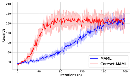
Figure 2: Reward comparison of Algorithm 1 and the vanilla MAML (Finn et al., 2017) on RL cart pole tasks.

Cart Pole: We evaluate Algorithm 1 in a deep meta-RL setting. In particular, we examine the cart pole environment (Towers et al., 2024), a classical control environment where physical properties of the system vary across tasks, including cart mass, pole mass, and pole length. The policy is parameterized by a multi-layer perceptron (MLP) architecture consisting of two hidden layers. Further details are provided in Appendix 6.9. Figure 2 shows the learning curves comparing Algorithm 1 with vanilla MAML (Finn et al., 2017), depicting both average rewards and standard deviations across 5 runs.

Our results demonstrate that Algorithm 1 learns approximately $3\times$ faster than the vanilla MAML algorithm, reaching higher reward values in fewer iterations. While our approach exhibits slightly higher variance (as indicated by the larger shaded regions representing standard deviation), it consistently outperforms the baseline in terms of learning speed. Notably, the task selection method reaches a reward of 150 around iteration $60$, whereas MAML takes approximately $200$ iterations to research the same reward. These empirical findings strongly support our theoretical analysis regarding sample complexity reduction (Corollary 1), validating that careful task selection significantly enhance sample-efficiency in meta-RL.

LQR: We follow the setting proposed by Toso et al. (2024b) to validate our theoretical guarantees in the MAML-LQR setting. In particular, Figure 3 (left) shows the optimality gap across iterations. We implemented the MAML-LQR on three scenarios: the full task pool (40 tasks), a selected subset (10 tasks), and two ablation baselines - selected subset without weight assignment and randomly selected subset. Our results demonstrate the faster convergence on the weighted selected subset, while both unweighted selected subset and random subset achieves at most the same performance as the full task pool. Moreover, Figure 3 (right) depicts the optimality gap between the selected subset and full task pool with respect to sample size, confirming our theoretical results on sample complexity reduction for the MAML-LQR (Corollary 2).

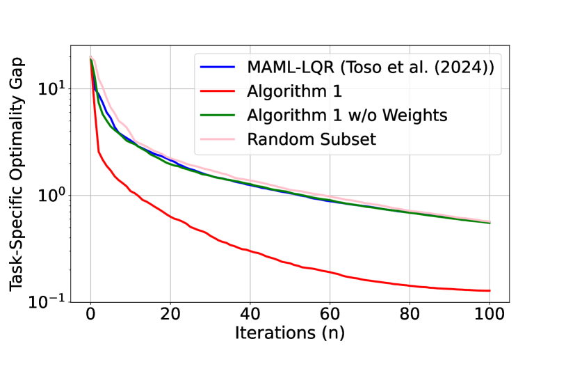
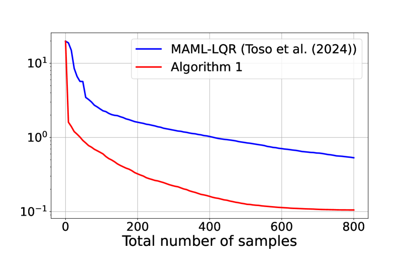
Figure 3: Optimality gap of Algorithm 1 in the MAML-LQR setting with respect to iterations.

5 Conclusions and Future Work

We proposed a coreset-based task selection to enhance sample efficiency in meta-RL. By prioritizing the most informative and diverse tasks, Algorithm 1 addressed the task redundancy of traditional meta-RL. We demonstrated that task selection reduces the sample complexity of finding $\epsilon$-near optimal solutions for both MAML-RL (i.e., by a factor of $\mathcal{O}(1/\epsilon)$) and MAML-LQR (i.e., proportional to $\mathcal{O}(\log(1/\epsilon))$), which are further validated through deep-RL and LQR experiments. Future work involves adding a clustering layer, as in Toso et al. (2023), based on the task weights, to the meta-training pipeline to alleviate the heterogeneity bias in the MAML-LQR setting.

6 Appendix

Roadmap: This appendix is organized as follows: First we extend our related work section and remind the reader of the model-agnostic meta-reinforcement learning problem and the matrix Bernstein inequality from Tropp (2012), where the later is crucial for controlling the error in the MAML gradient approximation due to the zeroth-order estimation. Next, in Section 6.3, we characterize that estimation error and prove that for a sufficiently large number of samples $n_{s}$, and sufficiently small smoothing radius $r$, the estimation error is composed of a sufficiently small error $\epsilon$ and an additive bias due to the task selection step in Algorithm 1, with high probability. Then, in Section 6.4 we derive the ergodic convergence rate of Algorithm 1 for the general setting of non-concave task-specific reward function $J_{i}(\theta)$. The sample complexity reduction benefit of task selection is then discussed in Section 6.5. In Sections 6.6, 6.7 and 6.8, we apply Algorithm 1 to the MAML-LQR problem where $J_{i}(\theta)$ satisfy a gradient dominance property. Finally in Section 6.9 we provide further details on the experimental setup considered in our numerical validation section.

6.1 Related Work

• Meta-Reinforcement Learning: There is a wealth of literature in meta-RL, with applications spanning robot manipulation (Yu et al., 2017; Arndt et al., 2020; Ghadirzadeh et al., 2021), robot locomotion (Song et al., 2020; Yu et al., 2020), build energy control (Luna Gutierrez and Leonetti, 2020), among others. Most relevant to our work are Song et al. (2019, 2020) that estimate the meta-gradient through evolutionary strategy. Similarly, we consider a zeroth-order estimation of the task-specific and meta-gradients. In contrast, these works treat all the tasks equally, leading to task redundancy which we handle with a derivative-free coreset learning approach to enhance data-efficiency in meta-RL.

• Meta-Reinforcement Learning Task Selection: Beyond the line of work on coresets for data-efficient training of machine learning models (Mirzasoleiman et al., 2020; Killamsetty et al., 2021; Yang et al., 2023; Pooladzandi et al., 2022; Balakrishnan et al., 2022), which use submodular optimization for subset selection, the works (Luna Gutierrez and Leonetti, 2020; Zhan and Anderson, 2024) are particularly relevant to this paper. In particular, Zhan and Anderson (2024) does not focus on RL tasks and approximates gradients using the pre-activation outputs of the last layer for classification tasks. That simplifies the problem but prevent them from deriving sample complexity guarantees. On the other hand, Shin et al. (2023) employs an information-theoretic metric to evaluate task similarities and relevance, considering a general MAML training framework rather than the policy gradient-based approach discussed here.

• Model-free Learning for Control: The linear quadratic regulator (LQR) problem has recently been taken as a fundamental baseline for establishing theoretical guarantees of policy optimization in control and reinforcement learning (Fazel et al., 2018). In particular, studies on multi-task and multi-agent learning for control (Zhang et al., 2023; Wang et al., 2023; Tang et al., 2023; Toso et al., 2024a, b; Lee et al., 2024a, b) have derived non-asymptotic guarantees for various learning architectures within the scope of model-free LQR. Most relevant to our work are Molybog and Lavaei (2021); Musavi and Dullerud (2023); Toso et al. (2024b); Aravind et al. (2024); Pan and Zhu (2024), which also study the meta-LQR problem and provide provable methods for learning meta-controllers that adapt quickly to unseen LQR tasks. In contrast to these works, we leverage the MAML-LQR problem as a case study to highlight the sample complexity reduction enabled by our embedded task selection approach.

6.2 Notation and Background Results

Notation: Let $[M]$ denote the set of integers $\{1,2,\ldots,M\}$, and $\rho(\cdot)$ the spectral radius of a square matrix. Let $\|\cdot\|$ and $\|\cdot\|_{F}$ denote the spectral and Frobenius norm, respectively. We use $\mathcal{O}(\cdot)$ to omit constant factors in the argument. Throughout the text and when its clear from the context we use $i$ and $j$ to denote tasks $T_{i}$ and $T_{j}$.

Model-Agnostic Meta-Reinforcement Learning Problem: We recall that the one-shot model-agnostic meta-reinforcement learning problem can be written as follows:

$$\theta^{\star}:=\text{argmax}_{\theta\in\Theta}J(\theta):=\mathbb{E}_{i\sim\mathcal{P}(\mathcal{T})}J_{i}(\theta+\eta_{\text{inn}}\nabla J_{i}(\theta)),$$

where $J_{i}(\theta):=\mathbb{E}_{\tau\sim\mathcal{P}_{i}(\tau|\theta)}[\mathcal{R}_{i}(\tau)]$, and $\eta_{\text{inn}}$ denotes some positive step-size.

Lemma 3 (Tropp (2012)).

(Matrix Bernstein Inequality) Let $\left\{Z_{l}\right\}_{l=1}^{m}$ be a set of $m$ independent random matrices of dimension $d=d_{1}\times d_{2}$ with $\mathbb{E}\left[Z_{l}\right]=Z$, $\left\|Z_{l}-Z\right\|\leq b$ almost surely, and maximum variance

$$\max\left(\left\|\mathbb{E}\left(Z_{l}Z_{l}^{\top}\right)-ZZ^{\top}\right\|,\left\|\mathbb{E}\left(Z_{l}^{\top}Z_{l}\right)-Z^{\top}Z\right\|\right)\leq\sigma^{2},$$

and sample average $\widehat{Z}:=\frac{1}{m}\sum_{l=1}^{m}Z_{l}$. Let a small tolerance $\epsilon\geq 0$ and small probability $0\leq\delta\leq 1$ be given. If

$$m\geq 2\left(\frac{\sigma^{2}}{\epsilon^{2}}+\frac{b}{3\epsilon}\right)\log\left(\frac{d_{1}+d_{2}}{\delta}\right)$$

$\text{ then }\mathbb{P}\left[\|\widehat{Z}-Z\|\leq\epsilon\right]\geq 1-\delta\text{.}$

Lemma 4 (Young’s inequality).

Given any two matrices $A,B\in\mathbb{R}^{d_{1}\times d_{2}}$ and a positive scalar $\nu$, it holds that

$$\|A+B\|_{2}^{2} \leq(1+\nu)\|A\|_{2}^{2}+\left(1+\frac{1}{\nu}\right)\|B\|_{2}^{2}\leq(1+\nu)\|A\|_{F}^{2}+\left(1+\frac{1}{\nu}\right)\|B\|_{F}^{2},$$ (9a)

$$\langle A,B\rangle \leq\frac{\nu}{2}\lVert A\rVert_{2}^{2}+\frac{1}{2\nu}\lVert B\rVert_{2}^{2}\leq\frac{\nu}{2}\lVert A\rVert_{F}^{2}+\frac{1}{2\nu}\lVert B\rVert_{F}^{2}.$$ (9b)

6.3 Gradient Estimation Error

Let $\tilde{J}(\theta):=\mathbb{E}_{u\sim\mathbb{S}_{r}}[J(\theta+u)]$ denote the Gaussian smoothing of the MAML reward function, with smoothing radius $r>0$ and $u$ being randomly drawn from a uniform distribution over matrices of dimension $d=d_{1}\times d_{2}$ and operator norm $r$, $\mathbb{S}_{r}$. By using the two-point zeroth-order estimation we can define the gradient of the smoothed MAML reward function as

$$\nabla\tilde{J}(\theta):=\mathbb{E}_{j,u}\left[\frac{d}{2r^{2}}\left(J_{j}(\theta+u+\eta_{\text{inn}}\nabla\tilde{J}_{j}(\theta+u))-J_{j}(\theta-u+\eta_{\text{inn}}\nabla\tilde{J}_{j}(\theta-u))\right)u\right],$$

where $\tilde{J}_{j}(\theta\pm u)=\mathbb{E}_{v\sim\mathbb{S}_{r}}[J_{j}(\theta\pm u+v)]$ denotes the Gaussian smoothing of the $i$-th task-specific expected reward function $J_{j}(\theta\pm u)$ incurred by the policy $\pi_{\theta\pm u}$. Note that the sample mean of $\nabla\tilde{J}(\theta)$ over tasks $i\sim\mathcal{P}(\mathcal{T})$ and samples $u\sim\mathbb{S}_{r}$ can be written as

$$\widetilde{\nabla}{J}(\theta):=\frac{d}{2Mn_{s}r^{2}}\sum_{j\in\mathcal{M}}\sum_{l=1}^{n_{s}}\left(J_{j}(\theta+u_{l}+\eta_{\text{inn}}\nabla\tilde{J}_{j}(\theta+u_{l}))-J_{j}(\theta-u_{l}+\eta_{\text{inn}}\nabla\tilde{J}_{j}(\theta-u_{l}))\right)u_{l}.$$

In addition, we define the two-point zeroth-order estimation of $\nabla J(\theta)$, over $\mathcal{M}$, as follows:

$$\nabla_{\mathcal{M}}{J}(\theta):=\frac{d}{2Mn_{s}r^{2}}\sum_{j\in\mathcal{M}}\sum_{l=1}^{n_{s}}\left(J_{j}(\theta+u_{l}+\eta_{\text{inn}}\widehat{\nabla}J_{j}(\theta))-J_{j}(\theta-u_{l}+\eta_{\text{inn}}\widehat{\nabla}J_{j}(\theta))\right)u_{l}$$

where

$$\widehat{\nabla}J_{j}(\theta):=\frac{d}{2n_{s}r^{2}}\sum_{l=1}^{n_{s}}\left(J_{j}(\theta+v_{l})-J_{j}(\theta-v_{l})\right)v_{l},$$

and similarly we can define the estimation over the subset of tasks $\mathcal{S}$ as

$$\nabla_{\mathcal{S}}{J}(\theta):=\frac{d}{2Mn_{s}r^{2}}\sum_{i\in\mathcal{S}}\gamma_{i}\sum_{l=1}^{n_{s}}\left(J_{i}(\theta+u_{l}+\eta_{\text{inn}}\widehat{\nabla}J_{i}(\theta))-J_{i}(\theta-u_{l}+\eta_{\text{inn}}\widehat{\nabla}J_{i}(\theta))\right)u_{l},$$

and define $g_{i}(\theta)=\frac{d}{2r^{2}n_{s}}\sum_{l=1}^{n_{s}}\left(J_{i}(\theta+u_{l}+\eta_{\text{inn}}\widehat{\nabla}J_{i}(\theta))-J_{i}(\theta-u_{l}+\eta_{\text{inn}}\widehat{\nabla}J_{i}(\theta))\right)u_{l}$.

Goal: We aim to demonstrate that the error in approximation of the gradient over the subset of tasks $\mathcal{S}$, i.e., $\|\nabla J(\theta)-\nabla_{\mathcal{S}}J(\theta)\|$, is sufficient small if the number of samples $n_{s}$, the smoothing radius $r$ and the step-size $\eta_{\text{inn}}$ are set accordingly. To do so, let us first write the following

$$\|\nabla J(\theta)-\nabla_{\mathcal{S}}J(\theta)\| =\|\nabla J(\theta)-\nabla_{\mathcal{M}}J(\theta)+\nabla_{\mathcal{M}}J(\theta)-\nabla_{\mathcal{S}}J(\theta)\|$$

$$\leq\underbrace{\|\nabla J(\theta)-\nabla_{\mathcal{M}}J(\theta)\|}_{\text{Zeroth-order gradient approximation}}+\underbrace{\|\nabla_{\mathcal{M}}J(\theta)-\nabla_{\mathcal{S}}J(\theta)\|}_{\text{Task selection}},$$

where we need to control the error in the gradient approximation over all the tasks in $\mathcal{M}$, and the error due to the task selection and training over the tasks in the subset $\mathcal{S}$.

$\bullet$ Zeroth-order gradient approximation $\|\nabla J(\theta)-\nabla_{\mathcal{M}}J(\theta)\|$:

$$\|\nabla J(\theta)-\nabla_{\mathcal{M}}J(\theta)\|\leq\underbrace{\|\nabla J(\theta)-\nabla\tilde{J}(\theta)\|}_{\textbf{(a)}}+\underbrace{\|\nabla\tilde{J}(\theta)-\widetilde{\nabla}J(\theta)\|}_{\textbf{(b)}}+\underbrace{\|\widetilde{\nabla}J(\theta)-\nabla_{\mathcal{M}}J(\theta)\|}_{(\textbf{c)}},$$

(a):

$$\|\nabla J(\theta)-\nabla\tilde{J}(\theta)\| =\|\mathbb{E}_{u\in\mathbb{S}_{r}}\left(\nabla J(\theta)-\nabla J(\theta+u)\right)\|$$

$$\stackrel{{\scriptstyle(i)}}{{\leq}}\mathbb{E}_{j,u}\|\nabla J_{j}(\theta+\eta_{\text{inn}}\nabla J_{j}(\theta))-\nabla J_{j}(\theta+u+\eta_{\text{inn}}\nabla J_{j}(\theta+u))\|$$

$$\stackrel{{\scriptstyle(ii)}}{{\leq}}\mathbb{E}_{j,u}\psi\|\eta_{\text{inn}}\left(\nabla J_{j}(\theta)-\nabla J_{j}(\theta+u)\right)-u\|$$

$$\leq\psi r(1+\psi\eta_{\text{inn}})\stackrel{{\scriptstyle(iii)}}{{\leq}}\frac{3\psi r}{2},$$

where $(i)$ and $(ii)$ follows from Jensen’s inequality and (6), respectively. Moreover, $(iii)$ follows from selecting the step-size according to $\eta_{\text{inn}}\leq\frac{1}{2\psi}$. Therefore, by selecting the smoothing radius as $r\leq\frac{2\epsilon}{9\psi}$, we obtain $\|\nabla J(\theta)-\nabla\tilde{J}(\theta)\|\leq\frac{\epsilon}{3}$.

(b): we first note that $\|\nabla\tilde{J}(\theta)-\widetilde{\nabla}J(\theta)\|=\|\mathbb{E}_{j,u}\widetilde{\nabla}J(\theta)-\widetilde{\nabla}J(\theta)\|$. In addition, since the tasks $T_{j}\in\mathcal{M}$ and samples $u\sim\mathbb{S}_{r}$ are drawn independently, we can use Lemma 3 to control $\|\nabla\tilde{J}(\theta)-\widetilde{\nabla}J(\theta)\|$. Let us first denote $Z_{l}=\frac{d}{2r^{2}}\left(J_{j}(\theta+u_{l}+\eta_{\text{inn}}\nabla\tilde{J}_{j}(\theta+u_{l}))-J_{j}(\theta-u_{l}+\eta_{\text{inn}}\nabla\tilde{J}_{j}(\theta-u_{l}))\right)u_{l}$ and $Z=\mathbb{E}_{j,u}[Z_{l}]$.

$$\|Z_{l}\| \leq\frac{d}{2r}|J_{j}(\theta+u_{l}+\eta_{\text{inn}}\nabla\tilde{J}_{j}(\theta+u_{l}))-J_{j}(\theta-u_{l}+\eta_{\text{inn}}\nabla\tilde{J}_{j}(\theta-u_{l}))|$$

$$\stackrel{{\scriptstyle(i)}}{{\leq}}\frac{d\beta J_{\max}}{2r}\|2u_{l}+\eta_{\text{inn}}\left(\nabla\tilde{J}_{j}(\theta+u_{l})-\nabla\tilde{J}_{j}(\theta-u_{l})\right)\|$$

$$\leq d\beta J_{\max}+\frac{d\beta J_{\max}\eta_{\text{inn}}}{2r}\|\mathbb{E}_{v\sim\mathbb{S}_{r}}\nabla J_{j}(\theta+u_{l}+v)-\nabla J_{j}(\theta-u_{l}+v)\|$$

$$\stackrel{{\scriptstyle(ii)}}{{\leq}}d\beta J_{\max}+\frac{d\beta J_{\max}\eta_{\text{inn}}\psi}{2r}\|2u_{j}\|\leq\frac{3d\beta J_{\max}}{2},$$

where $(i)$ is due to (6) and $J_{\max}=\max_{j\in\mathcal{M},\theta\in\Theta}J_{j}(\theta)$. In addition, $(ii)$ follows from the definition of the Gaussian smoothing of the task-specific reward function and from (6). The last inequality is due to $\eta_{\text{inn}}\leq\frac{1}{2\psi}$. Let us now control the approximation bias $\|Z_{l}-Z\|$.

$$\|Z\|=\|\nabla\tilde{J}(\theta)\|\leq\frac{\epsilon}{3}+\|\nabla J(\theta)\|\leq\frac{\epsilon}{3}+\phi,$$

which implies $\|Z_{l}-Z\|\leq\|Z_{l}\|+\|Z\|\leq b:=\frac{3d\beta J_{\max}}{2}+\frac{\epsilon}{3}+\phi$. We control the approximation variance $\|\mathbb{E}(Z_{l}Z_{l}^{\top})-ZZ^{\top}\|$ as follows:

$$\|\mathbb{E}(Z_{l}Z_{l}^{\top})-ZZ^{\top}\| \leq\|\mathbb{E}(Z_{l}Z_{l}^{\top})\|+\|ZZ^{\top}\|\leq\max_{Z_{l}}(\|Z_{l}\|)^{2}+\|Z\|^{2}$$

$$\leq\sigma^{2}:=\left(\frac{3d\beta J_{\max}}{2}\right)^{2}+\left(\frac{\epsilon}{3}+\phi\right)^{2},$$

and by selecting $Mn_{s}\geq 36\left(\frac{\sigma^{2}}{\epsilon^{2}}+\frac{b}{\epsilon}\right)\log\left(\frac{d_{1}+d_{2}}{\delta}\right)$, we have that $\|\nabla\tilde{J}(\theta)-\widetilde{\nabla}J(\theta)\|\leq\frac{\epsilon}{3}$ holds with probability $1-\delta$.

(c):

$$\|\widetilde{\nabla}J(\theta)-\nabla^{\prime}J(\theta)\|\leq\frac{d}{2Mn_{s}r^{2}}\sum_{j\in\mathcal{M}} \sum_{l=1}^{n_{s}}\|\left(J_{j}(\theta+u_{l}+\eta_{\text{inn}}\nabla\tilde{J}_{j}(\theta+u_{l}))-J_{j}(\theta+u_{l}+\eta_{\text{inn}}\widehat{\nabla}J_{j}(\theta))\right.$$

$$\left.+J_{j}(\theta-u_{l}+\eta_{\text{inn}}\widehat{\nabla}J_{j}(\theta))-J_{j}(\theta-u_{l}+\eta_{\text{inn}}\nabla\tilde{J}_{j}(\theta-u_{l}))\right)u_{l}\|$$

$$\hskip-71.13188pt\stackrel{{\scriptstyle(i)}}{{\leq}}\frac{d\beta J_{\max}\eta_{\text{inn}}}{2Mn_{s}r}\sum_{j\in\mathcal{M}}\sum_{l=1}^{n_{s}}\|\nabla\tilde{J}_{j}(\theta+u_{l})-\widehat{\nabla}J_{j}(\theta)\|+\|\nabla\tilde{J}_{j}(\theta-u_{l})-\widehat{\nabla}J_{j}(\theta)\|$$

$$\hskip-71.13188pt\stackrel{{\scriptstyle(ii)}}{{\leq}}d\beta J_{\max}\psi\eta_{\text{inn}}+\frac{d\beta J_{\max}\eta_{\text{inn}}}{Mn_{s}r}\sum_{j\in\mathcal{M}}\sum_{l=1}^{n_{s}}\|\nabla\tilde{J}_{j}(\theta)-\widehat{\nabla}J_{j}(\theta)\|,$$

where $(i)$ is due to (6), and $(ii)$ follows from adding and subtracting $\tilde{J}_{j}(\theta)$ and using (6) with the definition of Gaussian smoothing. Then, by (Flaxman et al., 2004, Lemma 1), $\nabla\tilde{J}_{j}(\theta)=\mathbb{E}_{u}[\frac{d}{r^{2}}J_{j}(\theta+u)u]$, which implies that $\nabla\tilde{J}_{j}(\theta)=\mathbb{E}\widehat{\nabla}J_{j}(\theta)=\mathbb{E}[\frac{d}{2r^{2}}\left(J_{j}(\theta+u)-J_{j}(\theta-u)\right)u]$ due to the symmetric perturbation of the two-point zeroth-order approximation. Therefore, we proceed to control $\|\nabla\tilde{J}_{j}(\theta)-\widehat{\nabla}J_{j}(\theta)\|=\|\mathbb{E}_{u}\widehat{\nabla}J_{j}(\theta)-\widehat{\nabla}J_{j}(\theta)\|$, by using Lemma 3 as previously. In particular, we define $Z_{l}=\frac{d}{2r^{2}}\left(J_{j}(\theta+u_{l})-J_{j}(\theta-u_{l})\right)u_{l}$ and $Z=\mathbb{E}_{u}[Z_{l}]$.

$$\|Z_{k}\| \leq\frac{d}{2r}|J_{j}(\theta+u_{l})-J_{j}(\theta-u_{l})|\stackrel{{\scriptstyle(i)}}{{\leq}}\frac{d\beta J_{\max}}{2r}\|2u_{l}\|\leq d\beta J_{\max},$$

where $(i)$ follows from (6). In addition, we have

$$\|Z\|=\|\nabla\tilde{J}_{j}(\theta)\| \leq\|\nabla\tilde{J}_{j}(\theta)-\nabla J_{j}(\theta)\|+\phi$$

$$\leq\mathbb{E}_{u}\|\nabla J_{j}(\theta+u)-\nabla J_{j}(\theta)\|+\phi$$

$$\leq\psi r+\phi\leq\frac{\epsilon}{3}+\phi,$$

where the last inequality follows from $r\leq\frac{\epsilon}{3\psi}$. Then, the approximation bias and variance of the estimation in (c) satisfy $\|Z_{k}-Z\|\leq b$ and $\|\mathbb{E}(Z_{k}Z_{k}^{\top})-ZZ^{\top}\|\leq\sigma^{2}$, respectively. This implies that, by selecting $n_{s}\geq 18\left(\frac{4\sigma^{2}}{\epsilon^{2}}+\frac{b}{\epsilon}\right)\log\left(\frac{d_{1}+d_{2}}{\delta}\right)$, $\|\nabla\tilde{J}_{j}(\theta)-\widehat{\nabla}J_{j}(\theta)\|\leq\frac{\epsilon}{6}$ holds with probability $1-\delta$. Finally, by setting the inner step-size as $\eta_{\text{inn}}\leq\min\left\{\frac{r}{d\beta J_{\max}},\frac{\epsilon}{6d\beta J_{\max}\psi}\right\}$, we have that $\|\widetilde{\nabla}J(\theta)-\nabla^{\prime}J(\theta)\|\leq\frac{\epsilon}{3}$ holds with probability $1-\delta$.

Therefore, by combining (a), (b) and (c), and supposing that the number of samples $n_{s}$, the smoothing radius $r$, and step-size $\eta_{\text{inn}}$ are set as follows:

$$n_{s}\geq 36\left(\frac{8\sigma^{2}}{\epsilon^{2}}+\frac{b}{\epsilon}\right)\log\left(\frac{d}{\delta}\right),r\leq\frac{\epsilon}{9\psi},\text{ and }\eta_{\text{inn}}\leq\min\left\{\frac{2r}{d\beta J_{\max}},\frac{1}{2\psi}\right\},$$

the zeroth-order estimation error is sufficiently small, i.e., $\|\nabla J(\theta)-\nabla_{\mathcal{M}}J(\theta)\|\leq\epsilon$ holds with probability $1-2\delta$.

It is worth noting that the number of samples, smoothing radius and inner step-size must be in the order of $n_{s}=\mathcal{O}(d^{2}/\epsilon^{2})$, $r=\mathcal{O}(\epsilon)$, and $\eta_{\text{inn}}=\mathcal{O}(\epsilon/d)$, respectively, in order to ensure that the estimation error due to the zeroth-order approximation is sufficiently small, i.e, $\|\nabla J(\theta)-\nabla_{\mathcal{M}}J(\theta)\|=\mathcal{O}(\epsilon)$. We use $\mathcal{O}(\cdot)$ to omit the dependence on universal constants and only highlight the scaling the number of samples with the problem dimension $d$ and approximation error $\epsilon$.

$\bullet$ Task Selection $\|\nabla_{\mathcal{M}}J(\theta)-\nabla_{\mathcal{S}}J(\theta)\|$: To control the estimation error due to the task selection, we start by writing the following

$$\|\nabla_{\mathcal{M}}J(\theta)-\nabla_{\mathcal{S}}J(\theta)\| =\left\|\frac{1}{M}\sum_{j\in\mathcal{M}}g_{j}(\theta)-\frac{1}{M}\sum_{i\in\mathcal{S}}\gamma_{i}g_{i}(\theta)\right\|=\frac{1}{M}\left\|\sum_{j\in\mathcal{M}}g_{j}(\theta)-\sum_{i\in\mathcal{S}}\gamma_{i}g_{i}(\theta)\right\|$$

$$\leq\frac{1}{M}\sum_{j\in\mathcal{M}}\min_{i\in\mathcal{S}}\left\|g_{j}(\theta)-g_{i}(\theta)\right\|\leq\frac{1}{M}\sum_{j\in\mathcal{M}}\min_{i\in\mathcal{S}}\max_{\theta\in\Theta}\left\|g_{j}(\theta)-g_{i}(\theta)\right\|.$$

We recall that the greedy subset selection (i.e., steps 2-10 in Algorithm 1) returns a subset $\mathcal{S}$ that is a suboptimal solution of the following submodular maximization

$$\mathcal{S}^{\star}=\underset{\mathcal{S}\subseteq\mathcal{M}}{\text{argmax}}\;\ \mathcal{F}(\mathcal{S}):=C-\sum_{j\in\mathcal{M}}\min_{i\in\mathcal{S}}\left\|{g}_{j}(\theta_{0})-g_{i}(\theta_{0})\right\|,\text{ subject to }|\mathcal{S}|\leq L,$$

for any $\theta_{0}\in\Theta$. In particular, by (Nemhauser et al., 1978, Section 4), we know that the value of the greedy optimization is close to the optimal as $\mathcal{F}(\mathcal{S})\geq(1-e^{-1})\mathcal{F}(\mathcal{S^{\star}})$. This implies that

$$\sum_{j\in\mathcal{M}}\min_{i\in\mathcal{S}}\left\|{g}_{j}(\theta_{0})-g_{i}(\theta_{0})\right\|\leq Ce^{-1}+(1-e^{-1})\sum_{j\in\mathcal{M}}\min_{i\in\mathcal{S^{\star}}}\left\|{g}_{j}(\theta_{0})-g_{i}(\theta_{0})\right\|,$$

and by taking the maximum of both sides with respect to $\theta\in\Theta$, we obtain

$$\frac{1}{M}\sum_{j\in\mathcal{M}}\min_{i\in\mathcal{S}}\max_{\theta\in\Theta}\left\|{g}_{j}(\theta)-g_{i}(\theta)\right\|\leq\frac{Ce^{-1}}{M}+\frac{(1-e^{-1})}{M}\sum_{j\in\mathcal{M}}\min_{i\in\mathcal{S^{\star}}}\max_{\theta\in\Theta}\left\|{g}_{j}(\theta)-g_{i}(\theta)\right\|,$$

where we control $\left\|{g}_{j}(\theta)-g_{i}(\theta)\right\|$ as follows

$$\left\|{g}_{j}(\theta)-g_{i}(\theta)\right\| \leq\left\|{g}_{j}(\theta)-\nabla J_{j}(\theta+\eta_{\text{inn}}\nabla J_{j}(\theta))\right\|+\left\|\nabla J_{j}(\theta+\eta_{\text{inn}}\nabla J_{j}(\theta))-\nabla J_{j}(\theta)\right\|$$

$$+\left\|{g}_{i}(\theta)-\nabla J_{i}(\theta+\eta_{\text{inn}}\nabla J_{i}(\theta))\right\|+\left\|\nabla J_{i}(\theta+\eta_{\text{inn}}\nabla J_{i}(\theta))-\nabla J_{i}(\theta)\right\|$$

$$+\|\nabla J_{i}(\theta)-\nabla J_{j}(\theta)\|$$

$$\stackrel{{\scriptstyle(i)}}{{\leq}}\left\|{g}_{j}(\theta)-\nabla J_{j}(\theta+\eta_{\text{inn}}\nabla J_{j}(\theta))\right\|+\left\|{g}_{i}(\theta)-\nabla J_{i}(\theta+\eta_{\text{inn}}\nabla J_{i}(\theta))\right\|$$

$$+2\eta_{\text{inn}}\psi\phi+\|\nabla J_{i}(\theta)-\nabla J_{j}(\theta)\|$$

$$\stackrel{{\scriptstyle(ii)}}{{\leq}}\left\|{g}_{j}(\theta)-\nabla J_{j}(\theta+\eta_{\text{inn}}\widehat{\nabla}J_{j}(\theta))\right\|+\left\|{g}_{i}(\theta)-\nabla J_{i}(\theta+\eta_{\text{inn}}\widehat{\nabla}J_{i}(\theta))\right\|$$

$$+\eta_{\text{inn}}\psi\|\widehat{\nabla}J_{j}(\theta)-\nabla J_{j}(\theta)\|+\eta_{\text{inn}}\psi\|\widehat{\nabla}J_{i}(\theta)-\nabla J_{i}(\theta)\|$$

$$+2\eta_{\text{inn}}\psi\phi+\|\nabla J_{i}(\theta)-\nabla J_{j}(\theta)\|,$$

where $(i)$ and $(ii)$ are due to (1). Therefore, we note that for either inner and outer zeroth-order gradient approximations, i.e., $\left\|{g}_{j}(\theta)-\nabla J_{j}(\theta+\eta_{\text{inn}}\widehat{\nabla}J_{j}(\theta))\right\|$ and $\|\widehat{\nabla}J_{j}(\theta)-\nabla J_{j}(\theta)\|$, respectively, the number of samples and smoothing radius can be set according to

$$n_{s}\geq C_{\text{approx},1}\left(\frac{\sigma^{2}}{\epsilon^{2}}+\frac{b}{3\epsilon}\right)\log\left(\frac{d_{1}+d_{2}}{\delta}\right),r\leq\frac{\epsilon}{C_{\text{approx},1}\psi}$$

to guarantee a small estimation error of $\epsilon$, with probability $1-\delta$, where $C_{\text{approx},1}$ is some positive universal constant, and $\sigma^{2}=\left(d\beta J_{\max}\right)^{2}+\left(\epsilon+\phi\right)^{2}$, $b=d\beta J_{\max}+\epsilon+\phi$. Therefore, following Definition 2, i.e., $\xi_{i,j}:=\max_{\theta\in\Theta}\|\nabla J_{i}(\theta)-\nabla J_{j}(\theta)\|$, the estimation error due to the task selection is bounded as follows:

$$\|\nabla_{\mathcal{M}}J(\theta)-\nabla_{\mathcal{M}}J(\theta)\|\leq\epsilon+\frac{1}{M}\sum_{j\in\mathcal{M}}\min_{i\in\mathcal{S^{\star}}}\xi_{i,j},$$

which holds with high probability $1-\delta$ for $n_{s}$ and $r$ as above, and $C\leq\frac{Me\epsilon}{C_{\text{approx},1}}$. Finally, the gradient estimation error $\|\nabla J(\theta)-\nabla_{\mathcal{S}}J(\theta)\|$ in Algorithm 1, is controlled by a sufficiently small error that comes from the zeroth-order estimation and an additive bias due to the task selection. That is,

$$\|\nabla J(\theta)-\nabla_{\mathcal{S}}J(\theta)\|\leq\epsilon+\frac{1}{M}\sum_{j\in\mathcal{M}}\min_{i\in\mathcal{S^{\star}}}\xi_{i,j},$$

which holds with high probability for $n_{s}=\mathcal{O}(d^{2}/\epsilon^{2})$, $r=\mathcal{O}(\epsilon)$, $\eta_{\text{inn}}=\mathcal{O}(\epsilon/d)$, and $C=\mathcal{O}(\epsilon)$. We emphasize that setting $C$ sufficiently small, i.e., $C=\mathcal{O}(\epsilon)$ is standard in the literature of coresets for data-efficient machine-learning (Mirzasoleiman et al., 2020; Pooladzandi et al., 2022; Yang et al., 2023) and it guarantees that the gradient estimation error due to the subset selection is sufficiently small.

Remark 1.

(Expected Reward vs Empirical Reward) It is worth noting that our previous derivations assume that we have access to an oracle that provides the task-specific expected reward $J_{j}(\theta)$ incurred by any policy $\pi_{\theta}$, with $\theta\in\Theta$. However, in practice, we often do not have access to the true distribution of trajectories conditioned on the policy, i.e., $\tau\sim\mathcal{P}_{i}(\tau|\theta)$, that is needed to compute $J_{j}(\theta)$. Therefore, one may approximate the expected reward $J_{j}(\theta)$ with an empirical reward $\hat{J}_{j}(\theta):=\frac{1}{n_{\tau}}\sum_{l=1}^{n_{\tau}}[\mathcal{R}_{j}(\tau_{l})]$, where $\{\tau_{l}\}^{n_{\tau}}_{l=1}$ are the trajectories obtained by playing with $\pi_{\theta}$, $n_{\tau}$ times. Note that, we can control the error between $J_{j}(\theta)$ and $\hat{J}_{j}(\theta)$ with $n_{\tau}$. Then, since that error should enters the analysis of Algorithm 1 for either with or without task selection settings, we may assume the access to $J_{j}(\theta)$, for simplicity, but we stress that our results can be readily extended to the practical setting of empirical rewards by controlling such error with a sufficiently large $n_{\tau}$.

6.4 Proof of Theorem 1 (ergodic Convergence Rate)

Recall that the meta-policy parameter is updated as follows:

$$\theta_{n+1}=\theta_{n}+\eta_{\text{out}}\nabla_{\mathcal{S}}J(\theta_{n})=\theta_{n}+\frac{\eta_{\text{out}}}{M}\sum_{i\in\mathcal{S}}\gamma_{i}g_{i}(\theta_{n}).$$

In addition, by using the definition of the meta-gradient and the gradient Lipschitz assumption (6), we have that

$$\|\nabla J(\theta_{1})-\nabla J(\theta_{2})\| =\|\mathbb{E}_{i}\nabla J_{i}(\theta_{1}+\eta_{\text{inn}}\nabla J_{i}(\theta_{1}))-\mathbb{E}_{i}\nabla J_{i}(\theta_{2}+\eta_{\text{inn}}\nabla J_{i}(\theta_{2}))\|$$

$$\stackrel{{\scriptstyle(i)}}{{\leq}}\mathbb{E}_{i}\psi\|(\theta_{1}-\theta_{2})+\eta_{\text{inn}}\left(\nabla J_{i}(\theta_{1})-\nabla J_{i}(\theta_{2})\right)\|$$

$$\leq\psi\|\theta_{1}-\theta_{2}\|+\eta_{\text{inn}}\|\nabla J_{i}(\theta_{1})-\nabla J_{i}(\theta_{2})\|$$

$$\stackrel{{\scriptstyle(ii)}}{{\leq}}\psi(1+\eta_{\text{inn}}\psi)\|\theta_{1}-\theta_{2}\|$$

$$\stackrel{{\scriptstyle(iii)}}{{\leq}}\frac{3\psi}{2}\|\theta_{1}-\theta_{2}\|=\overline{\psi}\|\theta_{1}-\theta_{2}\|,$$

for any $\theta_{1},\theta_{2}\in\Theta$. Here, $(i)$ and $(ii)$ follows from (2), and $(iii)$ is due to $\eta_{\text{inn}}\leq\frac{1}{4\psi}$. Therefore, the MAML reward function incurred by policy $\pi_{\theta}$ is $\overline{\psi}$-smooth and satisfy

$$J(\theta_{n})-J(\theta_{n+1}) \leq\langle\nabla J(\theta_{n}),\theta_{n}-\theta_{n+1}\rangle+\frac{\overline{\psi}}{2}\|\theta_{n+1}-\theta_{n}\|^{2}$$

$$=\langle\nabla J(\theta_{n}),-\eta_{\text{out}}\nabla_{\mathcal{S}}J(\theta_{n})+\eta_{\text{out}}{\nabla}J(\theta_{n})-\eta_{\text{out}}{\nabla}J(\theta_{n})\rangle+\frac{\eta_{\text{out}}^{2}\overline{\psi}}{2}\|\nabla_{\mathcal{S}}J(\theta_{n})\|^{2}$$

$$=-\eta_{\text{out}}\|\nabla J(\theta_{n})\|^{2}+\eta_{\text{out}}\langle\nabla J(\theta_{n}),\nabla J(\theta_{n})-\nabla_{\mathcal{S}}J(\theta_{n})\rangle+\frac{\eta_{\text{out}}^{2}\overline{\psi}}{2}\|\nabla_{\mathcal{S}}J(\theta_{n})\|^{2}$$

$$\stackrel{{\scriptstyle(i)}}{{\leq}}-\frac{\eta_{\text{out}}}{2}\|\nabla J(\theta_{n})\|^{2}+\frac{\eta_{\text{out}}}{2}\|\nabla J(\theta_{n})-\nabla_{\mathcal{S}}J(\theta_{n})\|^{2}+\frac{\eta_{\text{out}}^{2}\overline{\psi}}{2}\|\nabla_{\mathcal{S}}J(\theta_{n})\|^{2}$$

$$\stackrel{{\scriptstyle(ii)}}{{\leq}}-\frac{\eta_{\text{out}}}{2}\|\nabla J(\theta_{n})\|^{2}+\frac{\eta_{\text{out}}}{2}\|\nabla J(\theta_{n})-\nabla_{\mathcal{S}}J(\theta_{n})\|^{2}$$

$$+\eta_{\text{out}}^{2}\overline{\psi}\left(\|\nabla J(\theta_{n})\|^{2}+\|\nabla J(\theta_{n})-\nabla_{\mathcal{S}}J(\theta_{n})\|^{2}\right),$$

where $(i)$ and $(ii)$ follows from Young’s inequalities (9b) and (9a), respectively. Then, by setting $\eta_{\text{out}}\leq\frac{1}{2\overline{\psi}}$ and re-arranging the terms, we can write

$$\frac{\eta_{\text{out}}}{4}\|\nabla J(\theta_{n})\|^{2}_{2} \leq J(\theta_{n+1})-J(\theta_{n})+\frac{3\eta_{\text{out}}}{4}\|\nabla J(\theta_{n})-\nabla_{\mathcal{S}}J(\theta_{n})\|^{2},$$

which can be unrolled over the iterations $n=\{0,1,\ldots,N-1\}$ to obtain

$$\frac{1}{N}\sum_{n=0}^{N-1}\|\nabla J(\theta_{n})\|^{2}_{2} \leq\frac{4\Delta_{0}}{\eta_{\text{out}}N}+6\left(\frac{1}{M}\sum_{j\in\mathcal{M}}\min_{i\in\mathcal{S^{\star}}}\xi_{i,j}\right)^{2},$$

where we also use the fact that $J(\theta^{\star})\geq J(\theta_{N})$ above. In addition, we disregard $\mathcal{O}(\epsilon^{2})$ since it is negligible for small $\epsilon$. We also note that the first term denotes the local algorithm’s complexity to find an stationary solution given an initial optimality gap $\Delta_{0}=J(\theta^{\star})-J(\theta_{0})$, and the second term scales with the gradient approximation error due to the zeroth-order estimation and task selection. Therefore, by setting the number of iterations as $N=\mathcal{O}(1/\epsilon)$, Algorithm 1 satisfy

$$\frac{1}{N}\sum_{n=0}^{N-1}\|\nabla J(\theta_{n})\|^{2}_{2} \leq\mathcal{O}\left(\epsilon+\left(\frac{1}{M}\sum_{j\in\mathcal{M}}\min_{i\in\mathcal{S^{\star}}}\xi_{i,j}\right)^{2}\right).$$ (10)

6.5 Proof of Corollary 1 (Sample Complexity)

We let $\mathcal{S}^{\mathcal{S}}_{c}$ and $\mathcal{S}^{\mathcal{M}}_{c}$ denote the total number of samples required in Algorithm 1 to find an $\epsilon$-near stationary solution, with and without task selection, respectively. In particular, $\mathcal{S}^{\mathcal{S}}_{c}=\mathcal{O}\left(LNn_{s}\right)+\mathcal{O}\left(Mn_{s}\right)$ and $\mathcal{S}^{\mathcal{M}}_{c}=\mathcal{O}\left(MNn_{s}\right)$. Note that in order to guarantee (10) with high probability, we need $n_{s}=\mathcal{O}(d^{2}/\epsilon^{2})$ samples in the zeroth-order gradient estimation. Therefore, we have that $\mathcal{S}^{\mathcal{M}}_{c}=\mathcal{O}\left(MNn_{s}\right)=\mathcal{O}(d^{2}/\epsilon^{3})$, whereas $\mathcal{S}^{\mathcal{S}}_{c}=\frac{L}{M}\mathcal{O}\left(d^{2}/\epsilon^{3}\right)+\mathcal{O}\left(d^{2}/\epsilon^{2}\right).$ Then, for a sufficiently large amount of tasks in the task pool $\mathcal{M}$ (e.g., scaling as $M=\mathcal{O}(1/\epsilon)$) and a sufficiently small number of informative tasks in the subset $\mathcal{S}$, i.e., $L=\mathcal{O}(1)$, the task selection benefits from a sample complexity reduction by a factor of ${\color[rgb]{0,0,1}\mathcal{O}(1/\epsilon)}$ when compared to the setting without task selection.

6.6 Proof of Theorem 2 (Optimality Gap)

We first note Lemma 2 is provided in the Frobenius norm. Therefore, we use the fact that for any matrix $A\in\mathbb{R}^{d_{1}\times d_{2}}$, $\|A\|_{F}\leq\sqrt{\min(d_{1},d_{2})}\|A\|$, to adapt the gradient approximation error $\|\nabla J(\theta)-\nabla_{\mathcal{S}}J(\theta)\|$ as discussed previously in the RL setting, for the MAML-LQR where $\theta=K$ and $u\sim\mathbb{S}_{r}$ has Frobenius norm $r$ in ZO2P($\cdot$). Moreover, we recall that the meta-controller is updated as follows:

$$K_{n+1}=K_{n}-\eta_{\text{out}}\nabla_{\mathcal{S}}J(K_{n})=\theta_{n}-\frac{\eta_{\text{out}}}{M}\sum_{i\in\mathcal{S}}\gamma_{i}g_{i}(K_{n}),$$

where $g_{i}(K_{n})=\frac{d}{2r^{2}n_{s}}\sum_{l=1}^{n_{s}}\left(J_{i}(K_{n}+u_{l}-\eta_{\text{inn}}\widehat{\nabla}J_{i}(K_{n}))-J_{i}(K_{n}-u_{l}-\eta_{\text{inn}}\widehat{\nabla}J_{i}(K_{n}))\right)u_{l}$ for any task $T_{i}\sim\mathcal{P}(\mathcal{T})$. Then, by the gradient smoothness property in Lemma 2, we can write

$$J_{j}(K_{n+1}) -J_{j}(K_{n})\leq\langle\nabla J_{j}(K_{n}),K_{n+1}-K_{n}\rangle+\frac{\psi}{2}\|K_{n+1}-K_{n}\|^{2}_{F}$$

$$=\langle\nabla J_{j}(K_{n}),-\eta_{\text{out}}\nabla_{\mathcal{S}}J(K_{n})-\eta_{\text{out}}\nabla J_{j}(K_{n})+\eta_{\text{out}}\nabla J_{j}(K_{n})\rangle+\frac{\psi\eta_{\text{out}}^{2}}{2}\|\nabla_{\mathcal{S}}J(K_{n})\|^{2}_{F}$$

$$\leq-\frac{\eta_{\text{out}}}{2}\|\nabla J_{j}(K_{n})\|^{2}_{F}+\frac{\eta}{2}\|\nabla_{\mathcal{S}}J(K_{n})-\nabla J_{j}(K_{n})\|^{2}_{F}+\frac{\psi\eta_{\text{out}}^{2}}{2}\|\nabla_{\mathcal{S}}J(K_{n})\|^{2}_{F}$$

$$\leq-\frac{\eta_{\text{out}}}{4}\|{\nabla}J_{j}(K_{n})\|^{2}_{F}+\frac{3\eta_{\text{out}}}{4}\|\nabla_{\mathcal{S}}J(K_{n})-\nabla J_{j}(K_{n})\|^{2}_{F},$$

where the last two inequalities are due to Young’s inequality (9b) and (9a), and $\eta_{\text{out}}\leq\frac{1}{4\psi}$. Let us now proceed to control the error in the meta-gradient approximation over $\mathcal{S}$, i.e., $\nabla_{\mathcal{S}}J(K_{n})$, with respect to the task-specific gradient $\nabla J_{j}(K_{n})$.

$$\|\nabla_{\mathcal{S}}J(K_{n})-\nabla J_{j}(K_{n})\|_{F} \leq\underbrace{\left\|\nabla_{\mathcal{S}}J(K_{n})-\nabla J(K_{n})\right\|_{F}}_{\text{Gradient approximation}}+\underbrace{\left\|\nabla J(K_{n})-\nabla J_{j}(K_{n})\right\|_{F}}_{\text{Task heterogeneity}},$$

$\bullet$ Task heterogeneity:

$$\left\|\nabla J(K_{n})-\nabla J_{j}(K_{n})\right\|_{F}=\left\|\mathbb{E}_{i}\nabla J_{i}(K_{n}-\eta_{\text{inn}}\nabla J_{i}(K_{n}))-\nabla J_{j}(K_{n})\right\|_{F}$$

$$\leq\mathbb{E}_{i}\left\|\nabla J_{i}(K_{n}-\eta_{\text{inn}}\nabla J_{i}(K_{n}))-\nabla J_{i}(K_{n})+\nabla J_{i}(K_{n})-\nabla J_{j}(K_{n})\right\|_{F}$$

$$\leq\mathbb{E}_{i}\left\|\nabla J_{i}(K_{n}-\eta_{\text{inn}}\nabla J_{i}(K_{n}))-\nabla J_{i}(K_{n})\|_{F}+\mathbb{E}_{i}\|\nabla J_{i}(K_{n})-\nabla J_{j}(K_{n})\right\|_{F}$$

$$\stackrel{{\scriptstyle(i)}}{{\leq}}\eta_{\text{inn}}\psi\mathbb{E}_{i}\|\nabla J_{i}(K_{n})\|+\mathbb{E}_{i}\|\nabla J_{i}(K_{n})-\nabla J_{j}(K_{n})\|_{F}$$

$$\stackrel{{\scriptstyle(ii)}}{{\leq}}\eta_{\text{inn}}\psi\phi+f(\epsilon_{\text{het}}),$$

where $(i)$ is due to Lemma 2 and $(ii)$ follows from Lemmas 1 and 2.

$\bullet$ Gradient approximation:

$$\left\|\nabla_{\mathcal{S}}J(K_{n})-\nabla J(K_{n})\right\|_{F} =\left\|\nabla_{\mathcal{S}}J(K_{n})-\nabla_{\mathcal{M}}J(K_{n})+\nabla_{\mathcal{M}}J(K_{n})-\nabla J(K_{n})\right\|_{F}$$

$$\leq\underbrace{\left\|\nabla_{\mathcal{S}}J(K_{n})-\nabla_{\mathcal{M}}J(K_{n})\right\|_{F}}_{\text{Task selection}}+\underbrace{\|\nabla_{\mathcal{M}}J(K_{n})-\nabla J(K_{n})\|_{F}}_{\text{Zeroth-order approximation}}.$$

Following the previous analysis for the gradient estimation error of Algorithm 1 in Section 6.3, we know that $\left\|\nabla_{\mathcal{S}}J(K_{n})-\nabla J(K_{n})\right\|_{F}$ satisfy

$$\left\|\nabla_{\mathcal{S}}J(K_{n})-\nabla J(K_{n})\right\|_{F}\leq\epsilon+\frac{1}{M}\sum_{j\in\mathcal{M}}\min_{i\in\mathcal{S^{\star}}}\xi_{i,j},$$

with probability $1-\delta$, if the number of samples and smoothing radius are selected according to

$$n_{s}\geq C_{\text{approx},2}\min(d_{1},d_{2})\left(\frac{\sigma^{2}}{\epsilon^{2}}+\frac{b}{3\sqrt{\min(d_{1},d_{2})}\epsilon}\right)\log\left(\frac{d_{1}+d_{2}}{\delta}\right),r\leq\frac{\epsilon}{C_{\text{approx},2}\psi},$$ (11)

with $\eta_{\text{inn}}=\mathcal{O}(\epsilon)$ and $C=\mathcal{O}(\epsilon)$. We also note that $\min(d_{1},d_{2})$ and $\sqrt{\min(d_{1},d_{2})}$ come from the Frobenius norm in Lemma 2. Then, we can write

$$\hskip-2.84544ptJ_{j}(K_{n+1}) -J_{j}(K_{n})\hskip-2.84544pt\leq\hskip-2.84544pt-\frac{\eta_{\text{out}}}{4}\|{\nabla}J_{j}(K_{n})\|^{2}_{F}+3\eta_{\text{out}}\left(\eta_{\text{inn}}^{2}\psi^{2}\phi^{2}\hskip-2.84544pt+\hskip-2.84544ptf^{2}(\epsilon_{\text{het}})\hskip-2.84544pt+\hskip-2.84544pt\epsilon^{2}\hskip-2.84544pt+\hskip-2.84544pt\left(\frac{1}{M}\sum_{j\in\mathcal{M}}\min_{i\in\mathcal{S^{\star}}}\xi_{i,j}\right)^{2}\right)$$

$$\stackrel{{\scriptstyle(i)}}{{\leq}}-\frac{\lambda_{j}\eta_{\text{out}}}{4}\left(J_{j}(K_{n})-J_{j}(K^{\star}_{j})\right)+3\eta_{\text{out}}\left(f^{2}(\epsilon_{\text{het}})+\left(\frac{1}{M}\sum_{j\in\mathcal{M}}\min_{i\in\mathcal{S^{\star}}}\xi_{i,j}\right)^{2}\right)$$

$$\stackrel{{\scriptstyle(ii)}}{{\leq}}\frac{\lambda_{j}\eta_{\text{out}}}{4}\left(J_{j}(K_{n})-J_{j}(K^{\star}_{j})\right)+6\eta_{\text{out}}f^{2}(\epsilon_{\text{het}}),$$

where $(i)$ follows from the gradient dominance property in Lemma 2, $\eta_{\text{inn}}=\mathcal{O}(\epsilon)$ and disregarding $\mathcal{O}(\epsilon^{2})$ since it is negligible for small $\epsilon$. $(ii)$ is due to the fact that $\frac{1}{M}\sum_{j\in\mathcal{M}}\min_{i\in\mathcal{S}^{\star}}\xi_{i,j}\leq f(\epsilon_{\text{het}})$. Then, we can add and subtract $J_{j}(K^{\star}_{j})$ on the LHS to obtain

$$\Delta^{(j)}_{n+1}\leq\left(1-\frac{\lambda_{j}\eta_{\text{out}}}{4}\right)\Delta^{(j)}_{n}+6\eta_{\text{out}}f^{2}(\epsilon_{\text{het}}),$$

where $\Delta^{(j)}_{n}=J_{j}(K_{n})-J_{j}(K^{\star}_{j})$. Therefore, by unrolling the above expression over the iterations, $n=\{0,1,\ldots,N-1\}$, we obtain

$$\Delta^{(j)}_{N} \leq\left(1-\frac{\lambda_{j}\eta_{\text{out}}}{4}\right)^{N}\Delta^{(j)}_{0}+\frac{24}{\lambda_{j}}f^{2}(\epsilon_{\text{het}})\leq\epsilon+\frac{24}{\lambda_{j}}f^{2}(\epsilon_{\text{het}}),$$ (12)

where the last inequality is due to $N\geq\frac{4}{\eta_{\text{out}}\lambda_{j}}\log\left(\frac{\Delta^{(j)}_{0}}{\epsilon}\right)$. Then, we can conclude that Algorithm 1, for the MAML-LQR problem, learns a meta-controller $K_{N}$ that is $\epsilon$-close to any task-specific optimal controller (i.e., $T_{j}\sim\mathcal{P}(\mathcal{T})$) up to a task heterogeneity bias that scales as $\mathcal{O}\left(f^{2}(\epsilon_{\text{het}})\right)$.

6.7 Proof of Corollary 2 (Sample Complexity)

We let $\bar{\mathcal{S}}^{\mathcal{S}}_{c}$ and $\bar{\mathcal{S}}^{\mathcal{M}}_{c}$ to denote the total number of samples required in Algorithm 1, for the MAML-LQR problem, to learn a meta-controller $K_{N}$ that is $\epsilon$-close to any task-specific optimal controller up to a heterogeneity bias, with and without task selection, respectively. In particular, $\bar{\mathcal{S}}^{\mathcal{S}}_{c}=\mathcal{O}\left(LNn_{s}\right)+\mathcal{O}\left(Mn_{s}\right)$ and $\bar{\mathcal{S}}^{\mathcal{M}}_{c}=\mathcal{O}\left(MNn_{s}\right)$. In addition, to guarantee (12) with high probability, we need $n_{s}=\mathcal{O}(d^{2}/\epsilon^{2})$ samples in the zeroth-order gradient estimation. Therefore, $\bar{\mathcal{S}}^{\mathcal{M}}_{c}=\mathcal{O}\left(MNn_{s}\right)=\mathcal{O}((d^{2}/\epsilon^{2})\log(1/\epsilon))$, whereas $\bar{\mathcal{S}}^{\mathcal{S}}_{c}=\frac{L}{M}\mathcal{O}\left((d^{2}/\epsilon^{2})\log(1/\epsilon)\right)+\mathcal{O}\left(d^{2}/\epsilon^{2}\right),$ then, for a sufficiently large amount of tasks in the task pool $\mathcal{M}$ (e.g., scaling as $M=\mathcal{O}(\log(1/\epsilon))$) and a sufficiently small amount of tasks in the subset $\mathcal{S}$, i.e., $L=\mathcal{O}(1)$, the task selection may benefit from a sample complexity reduction of a factor of up to ${\color[rgb]{0,0,1}\mathcal{O}(\log(1/\epsilon))}$ when compared to the setting without task selection.

6.8 Stability Analysis

We now proceed to demonstrate that $K_{n}\in\mathcal{G}$, for any $n=\{0,1,\ldots,N-1\}$ of Algorithm 1. Let us first recall that by Assumption 4, the initial meta-controller is stabilizing, i.e., $K_{0}\in\mathcal{G}$. Then, we can first show that $\bar{K}_{0}=K_{0}-\eta_{\text{inn}}\widehat{\nabla}J_{j}(K_{0})$ and $K_{1}=K_{0}-\eta_{\text{out}}\nabla_{\mathcal{S}}J(K_{0})$ never leaves $\mathcal{G}$, with high probability, if the number of samples $n_{s}$, smoothing radius $r$, inner and outer step-sizes $\eta_{\text{inn}}$, $\eta_{\text{out}}$, and heterogeneity $f(\epsilon_{\text{text}})$ are set accordingly. Finally, we can use an induction step to extend the same for any iteration $n$. By the gradient smoothness in Lemma 2 we can write

$$J_{j}(\bar{K}_{0})-J_{j}(K_{0}) \leq-\frac{\eta_{\text{inn}}}{4}\|{\nabla}J_{j}(K_{0})\|^{2}_{F}+\frac{3\eta_{\text{inn}}}{4}\|\widehat{\nabla}J_{j}(K_{0})-\nabla J_{j}(K_{0})\|^{2}_{F},$$

where $\eta_{\text{out}}\leq\frac{1}{4\psi}$. Then, by using the gradient dominance property we have that

$$J_{j}(\bar{K}_{0})-J_{j}(K^{\star}_{j}) \leq\left(1-\frac{\lambda_{j}\eta_{\text{inn}}}{4}\right)\Delta^{(j)}_{0}+\frac{3\eta_{\text{inn}}}{4}\|\widehat{\nabla}J_{j}(K_{0})-\nabla J_{j}(K_{0})\|^{2}_{F},$$

where $\|\widehat{\nabla}J_{j}(K_{0})-\nabla J_{j}(K_{0})\|^{2}_{F}$ corresponds to the zeroth-order gradient estimation error at $K_{0}$. As well-established in (Toso et al., 2024b, a) and also discussed previously in this work, the zeroth-order estimation error can be made arbitrarily small, for instance, $\|\widehat{\nabla}J_{j}(K_{0})-\nabla J_{j}(K_{0})\|_{F}\leq\sqrt{\frac{\lambda_{j}\Delta^{(j)}_{0}}{6}}$, for $n_{s}=\mathcal{O}\left(\frac{6\psi}{\lambda_{j}}\right)$ and $r=\mathcal{O}\left(\sqrt{\frac{\lambda_{j}\Delta^{(j)}_{0}}{6}}\right)$. Then, for all tasks $T_{j}\sim\mathcal{P}(\mathcal{T})$ we have

$$J_{j}(\bar{K}_{0})-J_{j}(K^{\star}_{j}) \leq\left(1-\frac{\lambda_{j}\eta_{\text{inn}}}{8}\right)\Delta^{(j)}_{0},$$

which implies that $K_{0}\in\mathcal{G}$ (i.e., see Definition 3). We proceed to show that $K_{1}\in\mathcal{G}$. To do so, we use again the gradient smoothness in Lemma 2 to write

$$J_{j}(K_{1}) -J_{j}(K_{0})\leq-\frac{\eta_{\text{out}}}{4}\|{\nabla}J_{j}(K_{0})\|^{2}_{F}+\frac{3\eta_{\text{out}}}{4}\|\nabla_{\mathcal{S}}J(K_{0})-\nabla J_{j}(K_{0})\|^{2}_{F}$$

$$\stackrel{{\scriptstyle(i)}}{{\leq}}-\frac{\eta_{\text{out}}}{4}\|{\nabla}J_{j}(K_{0})\|^{2}_{F}+\frac{3\eta_{\text{out}}}{2}\|\nabla_{\mathcal{S}}J(K_{0})-\nabla J(K_{0})\|^{2}_{F}+3\eta_{\text{out}}f^{2}(\epsilon_{\text{het}})+3\eta_{\text{out}}\eta^{2}_{\text{inn}}\phi^{2},$$

where $(i)$ is due to Young’s inequality (9a) and

$$\|\nabla J(K_{0})-J_{j}(K_{0})\|^{2}_{F}\leq\mathbb{E}_{i}\|\nabla J_{i}(K_{0}-\eta_{\text{inn}}\nabla J_{i}(K_{0}))-\nabla J_{j}(K_{0})\|^{2}_{F}\leq 2\eta^{2}_{\text{inn}}\phi^{2}+2f^{2}(\epsilon_{\text{het}}).$$

Then, by the gradient dominance property we have that

$$J_{j}(K_{1})-J_{j}(K^{\star}_{j}) \leq\left(1-\frac{\lambda_{j}\eta_{\text{out}}}{4}\right)\Delta^{(j)}_{0}+\frac{3\eta_{\text{out}}}{2}\|\nabla_{\mathcal{S}}J(K_{0})-\nabla J(K_{0})\|^{2}_{F}$$

$$+3\eta_{\text{out}}f^{2}(\epsilon_{\text{het}})+3\eta_{\text{out}}\eta^{2}_{\text{inn}}\phi^{2},$$

where the gradient estimation error $\|\nabla_{\mathcal{S}}J(K_{0})-\nabla J(K_{0})\|_{F}$ satisfy

$$\|\nabla_{\mathcal{S}}J(K_{0})-\nabla J(K_{0})\|_{F}\leq\zeta+\frac{1}{M}\sum_{j\in\mathcal{M}}\min_{i\in\mathcal{S^{\star}}}\xi_{i,j}\leq\zeta+f(\epsilon_{\text{het}}),$$

with probability $1-\delta$, for $n_{s}$ and $r$ satisfying (11) with $\zeta$ in lieu of $\epsilon$. Then, we can write

$$J_{j}(K_{1})-J_{j}(K^{\star}_{j}) \leq\left(1-\frac{\lambda_{j}\eta_{\text{out}}}{4}\right)\Delta^{(j)}_{0}+3\eta_{\text{out}}\zeta^{2}+6\eta_{\text{out}}f^{2}(\epsilon_{\text{het}})+3\eta_{\text{out}}\eta^{2}_{\text{inn}}\phi^{2}$$

$$\stackrel{{\scriptstyle(i)}}{{\leq}}\left(1-\frac{\lambda_{j}\eta_{\text{out}}}{8}\right)\Delta^{(j)}_{0}$$

where $(i)$ follows from $\zeta=\sqrt{\frac{\lambda_{j}\Delta^{(j)}_{0}}{72}}$, $f(\epsilon_{\text{het}})\leq\frac{\lambda_{j}\Delta^{(j)}_{0}}{72}$, and $\eta_{\text{inn}}\leq\sqrt{\frac{\lambda_{j}\Delta^{(j)}_{0}}{72\phi^{2}}}$, which implies that $K_{1}\in\mathcal{G}$. Therefore, we define our base case and inductive hypothesis as follows:

$$\textbf{Base case:}\;\ J_{j}(\bar{K}_{0})-J_{j}(K^{\star}_{j}) \leq J_{j}(K_{0})-J_{j}(K^{\star}_{j}),$$

$$J_{j}(K_{1})-J_{j}(K^{\star}_{j}) \leq J_{j}(K_{0})-J_{j}(K^{\star}_{j})$$

$$\textbf{Inductive hypothesis:}\;\ J_{j}(\bar{K}_{n})-J_{j}(K^{\star}_{j}) \leq J_{j}(K_{0})-J_{j}(K^{\star}_{j}),$$

$$J_{j}(K_{n})-J_{j}(K^{\star}_{j}) \leq J_{j}(K_{0})-J_{j}(K^{\star}_{j})$$

which can be used along with the aforementioned conditions on the number of samples, smoothing radius, step-sizes and heterogeneity, to write

$$J_{j}(K_{n+1})-J_{j}(K^{\star}_{j}) \leq\left(1-\frac{\lambda_{j}\eta_{\text{out}}}{4}\right)\Delta^{(j)}_{n}+3\eta_{\text{out}}\zeta^{2}+6\eta_{\text{out}}f^{2}(\epsilon_{\text{het}})+3\eta_{\text{out}}\eta^{2}_{\text{inn}}\phi^{2}$$

$$\stackrel{{\scriptstyle(i)}}{{\leq}}\left(1-\frac{\lambda_{j}\eta_{\text{out}}}{8}\right)\Delta^{(j)}_{0}\leq\Delta^{(j)}_{0},$$

which guarantees that Algorithm 1 produces MAML stabilizing controllers with high probability.

6.9 Numerical Validation

Cart Pole: In this experiment, we configured the cart pole environment with parameters uniformly sampled from predefined intervals: cart mass from [0.8, 1.2], pole mass from [0.08, 0.12], and pole length from [0.4, 0.6]. We maintained an episodic task pool of 800 tasks with a selection ratio of 25%. The learning rates were set to 0.2 for the inner loop and 0.05 for the meta-learning process. For each iteration, we used a batch size of 20 tasks. All experiments were implemented using PyTorch, OpenAI Gym (Towers et al., 2024), running on an NVIDIA GeForce 3090 GPU with 90GB RAM. We compared the wall-clock running time between our proposed task selection algorithm and vanilla MAML. The average per-iteration running time was 3.32s for the task selection algorithm and 2.89s for vanilla MAML, demonstrating that our approach achieves significantly faster convergence while maintaining comparable computational efficiency.

Hopper: For the hopper environment, we configured the task sampling with mass scale from [0.9, 1.1] and friction coefficient scale from [0.9, 1.1]. We maintained an episodic task pool of 800 tasks with a selection ratio of 25%. The learning rates were set to 0.1 for the inner loop with 3 adaptation steps and 0.08 for the meta-learning process. For each iteration, we used a batch size of 10 tasks. All experiments were implemented using PyTorch, OpenAI Gym (Towers et al., 2024) and Mujoco (Todorov et al., 2012), running on an NVIDIA GeForce 3090 GPU with 90GB RAM. The average per-iteration running time was 3.72s for the task selection algorithm and 3.35s for vanilla MAML.

References

- Aravind et al. (2024) A. Aravind, M. T. Toghani, and C. A. Uribe. A Moreau envelope approach for LQR meta-policy estimation. arXiv preprint arXiv:2403.17364, 2024.
- Arndt et al. (2020) K. Arndt, M. Hazara, A. Ghadirzadeh, and V. Kyrki. Meta reinforcement learning for sim-to-real domain adaptation. In 2020 IEEE international conference on robotics and automation (ICRA), pages 2725–2731. IEEE, 2020.
- Balakrishnan et al. (2022) R. Balakrishnan, T. Li, T. Zhou, N. Himayat, V. Smith, and J. Bilmes. Diverse client selection for federated learning via submodular maximization. In International Conference on Learning Representations, 2022.
- Cornuejols et al. (1977) G. Cornuejols, M. Fisher, and G. L. Nemhauser. On the uncapacitated location problem. In Annals of Discrete Mathematics, volume 1, pages 163–177. Elsevier, 1977.
- Duan et al. (2016) Y. Duan, J. Schulman, X. Chen, P. L. Bartlett, I. Sutskever, and P. Abbeel. : Fast reinforcement learning via slow reinforcement learning. arXiv preprint arXiv:1611.02779, 2016.
- Fazel et al. (2018) M. Fazel, R. Ge, S. Kakade, and M. Mesbahi. Global convergence of policy gradient methods for the linear quadratic regulator. In International conference on machine learning, pages 1467–1476. PMLR, 2018.
- Finn et al. (2017) C. Finn, P. Abbeel, and S. Levine. Model-agnostic meta-learning for fast adaptation of deep networks. In International conference on machine learning, pages 1126–1135. PMLR, 2017.
- Flaxman et al. (2004) A. D. Flaxman, A. T. Kalai, and H. B. McMahan. Online convex optimization in the bandit setting: gradient descent without a gradient. arXiv preprint cs/0408007, 2004.
- Ghadirzadeh et al. (2021) A. Ghadirzadeh, X. Chen, P. Poklukar, C. Finn, M. Björkman, and D. Kragic. Bayesian meta-learning for few-shot policy adaptation across robotic platforms. In 2021 IEEE/RSJ International Conference on Intelligent Robots and Systems (IROS), pages 1274–1280. IEEE, 2021.
- Gravell et al. (2020) B. Gravell, P. M. Esfahani, and T. Summers. Learning optimal controllers for linear systems with multiplicative noise via policy gradient. IEEE Transactions on Automatic Control, 66(11):5283–5298, 2020.
- Killamsetty et al. (2021) K. Killamsetty, G. Ramakrishnan, A. De, and R. Iyer. Grad-match: Gradient matching based data subset selection for efficient deep model training. In International Conference on Machine Learning, pages 5464–5474. PMLR, 2021.
- Lee et al. (2024a) B. Lee, A. Rantzer, and N. Matni. Nonasymptotic regret analysis of adaptive linear quadratic control with model misspecification. In 6th Annual Learning for Dynamics & Control Conference, pages 980–992. PMLR, 2024a.
- Lee et al. (2024b) B. D. Lee, L. F. Toso, T. T. Zhang, J. Anderson, and N. Matni. Regret analysis of multi-task representation learning for linear-quadratic adaptive control. arXiv preprint arXiv:2407.05781, 2024b.
- Li et al. (2019) X. Li, K. Huang, W. Yang, S. Wang, and Z. Zhang. On the convergence of fedavg on non-iid data. arXiv preprint arXiv:1907.02189, 2019.
- Liu et al. (2022) C. Liu, L. Zhu, and M. Belkin. Loss landscapes and optimization in over-parameterized non-linear systems and neural networks. Applied and Computational Harmonic Analysis, 59:85–116, 2022.
- Liu et al. (2019) H. Liu, R. Socher, and C. Xiong. Taming maml: Efficient unbiased meta-reinforcement learning. In International conference on machine learning, pages 4061–4071. PMLR, 2019.
- Luna Gutierrez and Leonetti (2020) R. Luna Gutierrez and M. Leonetti. Information-theoretic task selection for meta-reinforcement learning. Advances in Neural Information Processing Systems, 33:20532–20542, 2020.
- Malik et al. (2019) D. Malik, A. Pananjady, K. Bhatia, K. Khamaru, P. Bartlett, and M. Wainwright. Derivative-free methods for policy optimization: Guarantees for linear quadratic systems. In The 22nd international conference on artificial intelligence and statistics, pages 2916–2925. PMLR, 2019.
- Mirzasoleiman et al. (2020) B. Mirzasoleiman, J. Bilmes, and J. Leskovec. Coresets for data-efficient training of machine learning models. In International Conference on Machine Learning, pages 6950–6960. PMLR, 2020.
- Molybog and Lavaei (2021) I. Molybog and J. Lavaei. When does maml objective have benign landscape? In 2021 IEEE Conference on Control Technology and Applications (CCTA), pages 220–227. IEEE, 2021.
- Musavi and Dullerud (2023) N. Musavi and G. E. Dullerud. Convergence of Gradient-based MAML in LQR. arXiv preprint arXiv:2309.06588, 2023.
- Nagabandi et al. (2018) A. Nagabandi, I. Clavera, S. Liu, R. S. Fearing, P. Abbeel, S. Levine, and C. Finn. Learning to adapt in dynamic, real-world environments through meta-reinforcement learning. arXiv preprint arXiv:1803.11347, 2018.
- Nemhauser et al. (1978) G. L. Nemhauser, L. A. Wolsey, and M. L. Fisher. An analysis of approximations for maximizing submodular set functions. Mathematical programming, 14(1):265–294, 1978.
- Nesterov and Spokoiny (2017) Y. Nesterov and V. Spokoiny. Random gradient-free minimization of convex functions. Foundations of Computational Mathematics, 17:527–566, 2017.
- Oymak and Soltanolkotabi (2019) S. Oymak and M. Soltanolkotabi. Overparameterized nonlinear learning: Gradient descent takes the shortest path? In International Conference on Machine Learning, pages 4951–4960. PMLR, 2019.
- Pan and Zhu (2024) Y. Pan and Q. Zhu. Model-agnostic zeroth-order policy optimization for meta-learning of ergodic linear quadratic regulators. arXiv preprint arXiv:2405.17370, 2024.
- Pooladzandi et al. (2022) O. Pooladzandi, D. Davini, and B. Mirzasoleiman. Adaptive second order coresets for data-efficient machine learning. In International Conference on Machine Learning, pages 17848–17869. PMLR, 2022.
- Rothfuss et al. (2018) J. Rothfuss, D. Lee, I. Clavera, T. Asfour, and P. Abbeel. Promp: Proximal meta-policy search. arXiv preprint arXiv:1810.06784, 2018.
- Salimans et al. (2017) T. Salimans, J. Ho, X. Chen, S. Sidor, and I. Sutskever. Evolution strategies as a scalable alternative to reinforcement learning. arXiv preprint arXiv:1703.03864, 2017.
- Shin et al. (2023) J. Shin, G. Kim, H. Lee, J. Han, and I. Yang. On task-relevant loss functions in meta-reinforcement learning and online LQR. arXiv preprint arXiv:2312.05465, 2023.
- Song et al. (2019) X. Song, W. Gao, Y. Yang, K. Choromanski, A. Pacchiano, and Y. Tang. ES-MAML: Simple Hessian-free meta learning. arXiv preprint arXiv:1910.01215, 2019.
- Song et al. (2020) X. Song, Y. Yang, K. Choromanski, K. Caluwaerts, W. Gao, C. Finn, and J. Tan. Rapidly adaptable legged robots via evolutionary meta-learning. In 2020 IEEE/RSJ International Conference on Intelligent Robots and Systems (IROS), pages 3769–3776. IEEE, 2020.
- Spall (2005) J. C. Spall. Introduction to stochastic search and optimization: estimation, simulation, and control. John Wiley & Sons, 2005.
- Stein (1972) C. Stein. A bound for the error in the normal approximation to the distribution of a sum of dependent random variables. In Proceedings of the Sixth Berkeley Symposium on Mathematical Statistics and Probability, Volume 2: Probability Theory, volume 6, pages 583–603. University of California Press, 1972.
- Stich (2018) S. U. Stich. Local SGD converges fast and communicates little. arXiv preprint arXiv:1805.09767, 2018.
- Tang et al. (2023) Y. Tang, Z. Ren, and N. Li. Zeroth-order feedback optimization for cooperative multi-agent systems. Automatica, 148:110741, 2023.
- Tiwari et al. (2022) R. Tiwari, K. Killamsetty, R. Iyer, and P. Shenoy. GCR: Gradient coreset based replay buffer selection for continual learning. In Proceedings of the IEEE/CVF Conference on Computer Vision and Pattern Recognition, pages 99–108, 2022.
- Todorov et al. (2012) E. Todorov, T. Erez, and Y. Tassa. Mujoco: A physics engine for model-based control. In 2012 IEEE/RSJ International Conference on Intelligent Robots and Systems, pages 5026–5033. IEEE, 2012. doi: 10.1109/IROS.2012.6386109.
- Toso et al. (2023) L. F. Toso, H. Wang, and J. Anderson. Learning personalized models with clustered system identification. In 2023 62nd IEEE Conference on Decision and Control (CDC), pages 7162–7169. IEEE, 2023.
- Toso et al. (2024a) L. F. Toso, H. Wang, and J. Anderson. Asynchronous Heterogeneous Linear Quadratic Regulator Design. arXiv preprint arXiv:2404.09061, 2024a.
- Toso et al. (2024b) L. F. Toso, D. Zhan, J. Anderson, and H. Wang. Meta-learning linear quadratic regulators: A policy gradient MAML approach for model-free LQR. Proceedings of the 6th Annual Learning for Dynamics & Control Conference, 242:902–915, 15–17 Jul 2024b.
- Towers et al. (2024) M. Towers, A. Kwiatkowski, J. Terry, J. U. Balis, G. De Cola, T. Deleu, M. Goulao, A. Kallinteris, M. Krimmel, A. KG, et al. Gymnasium: A standard interface for reinforcement learning environments. arXiv preprint arXiv:2407.17032, 2024.
- Tropp (2012) J. A. Tropp. User-friendly tail bounds for sums of random matrices. Foundations of computational mathematics, 12:389–434, 2012.
- Wang et al. (2023) H. Wang, L. F. Toso, A. Mitra, and J. Anderson. Model-free Learning with Heterogeneous Dynamical Systems: A Federated LQR Approach. arXiv preprint arXiv:2308.11743, 2023.
- Wang et al. (2016) J. X. Wang, Z. Kurth-Nelson, D. Tirumala, H. Soyer, J. Z. Leibo, R. Munos, C. Blundell, D. Kumaran, and M. Botvinick. Learning to reinforcement learn. arXiv preprint arXiv:1611.05763, 2016.
- Wang et al. (2022) Z. Wang, L. Shen, T. Duan, D. Zhan, L. Fang, and M. Gao. Learning to learn and remember super long multi-domain task sequence. In Proceedings of the IEEE/CVF Conference on Computer Vision and Pattern Recognition, pages 7982–7992, 2022.
- Wolsey (1982) L. A. Wolsey. An analysis of the greedy algorithm for the submodular set covering problem. Combinatorica, 2(4):385–393, 1982.
- Yang et al. (2023) Y. Yang, H. Kang, and B. Mirzasoleiman. Towards sustainable learning: Coresets for data-efficient deep learning. arXiv preprint arXiv:2306.01244, 2023.
- Yu et al. (2017) W. Yu, J. Tan, C. K. Liu, and G. Turk. Preparing for the unknown: Learning a universal policy with online system identification. arXiv preprint arXiv:1702.02453, 2017.
- Yu et al. (2020) W. Yu, J. Tan, Y. Bai, E. Coumans, and S. Ha. Learning fast adaptation with meta strategy optimization. IEEE Robotics and Automation Letters, 5(2):2950–2957, 2020.
- Zhan and Anderson (2024) D. Zhan and J. Anderson. Data-efficient and robust task selection for meta-learning. In Proceedings of the IEEE/CVF Conference on Computer Vision and Pattern Recognition (CVPR) Workshops, pages 8056–8065, June 2024.
- Zhang et al. (2023) T. T. Zhang, K. Kang, B. D. Lee, C. Tomlin, S. Levine, S. Tu, and N. Matni. Multi-task imitation learning for linear dynamical systems. In Learning for Dynamics and Control Conference, pages 586–599. PMLR, 2023.