Rational Motions of Minimal Quaternionic Degree with Prescribed Plane Trajectories

Abstract

This paper investigates the construction of rational motions of a minimal quaternionic degree that generate a prescribed plane trajectory (a “rational torse”). Using the algebraic framework of dual quaternions, we formulate the problem as a system of polynomial equations. We derive necessary and sufficient conditions for the existence of such motions, establish a method to compute solutions and characterize solutions of minimal degree. Our findings reveal that a rational torse is realizable as a trajectory of a rational motion if and only if its Gauss map is rational. Furthermore, we demonstrate that the minimal degree of a motion polynomial is geometrically related to a drop of degree of the Gauss and algebraically determined by the structure of the torse’s associated plane polynomial and the real greatest common divisor of its vector part. The developed theoretical framework has potential applications in robotics, computer-aided design, and computational kinematic, offering a systematic approach to constructing rational motions of small algebraic complexity.

1 Introduction

It is common to design a rigid body motion by prescribing one of its point trajectories [1, 2, 3]. But one can also imagine situations when the trajectory of a plane is to be created by a motion. A single point trajectory curve does not constrain at all the orientation along the curve while a plane trajectory partially constrains position and orientation. Thus, there is an infinity of motions along a certain point or plane trajectory and one can ask the question of how to sensible use these degrees of freedom?

In this paper we consider rational rigid body motions of Euclidean three-space with a prescribed rational plane trajectory (a rational torse). We provide answers to the following questions:

• Under which conditions on the rational torse do such rigid body motions exist?

• What is the minimal possible motion degree that can be achieved?

• Under which conditions is this minimal motion essentially unique?

Here, the notion of degree refers to the representation of rigid body motions in the dual quaternion model of space kinematics (the “quaternion degree” in the sense of [4]). It is different from the more common degree with respect to the parametrization of $\operatorname{SE}(3)$ by homogeneous transformation matrices [4]. However, our notion of degree is arguably more relevant when it comes to the construction of mechanisms to perform a prescribed motion [5, 6]. “Essential uniqueness” means uniqueness in a geometric sense, up to coordinate changes in the moving frame, that is, up to right multiplication with constant rigid body displacements.

While point trajectories in kinematics have been investigated extensively, much less in known for the trajectory of planes (and of lines). A standard reference on theoretical kinematics features a short section on that topic [7, Section VI.7]. The paper [8] studies rigid body transformations of points, lines, and planes in a Clifford algebra setting and discusses examples from computer vision and geometric constraint solving. An additional motivation to study the kinematics of plane trajectories is the close relation between torses and developable surface [9].

Our research questions are motivated by a similar investigation in [10] on minimal degree motions with a prescribed point trajectory $\gamma(t)$. The main results of that paper are as follows:

• The minimal degree motion to a rational curve is essentially unique in all cases.

• In generic cases the minimal achievable motion degree equals the curve degree and the minimal degree motion is the trivial curvilinear translation along the curve.

• If the curve is of circularity $c>0$ (refer to [10] for a definition of that concept) the minimal motion degree is $\deg\gamma(t)-c$ and the motion itself is the superposition of a translation along the curve $\gamma(t)$ with some change of orientation.

The minimal degree motion was used in [6] for a construction of exceptionally simple Kempe linkages for rational curves. In similar spirit, we may ask for linkages to produce a rational plane trajectory. This is an open question and its solution will require properties of rational motions of minimal degree with a given plane trajectory. Results of this article will show that there are substantial differences to the curve case:

• Rational motions with prescribed rational torse exist if and only if the torse has a rational Gauss image $n$. This is not always the case.

• Generically, the minimal achievable motion degree is half the torse degree. It increases if there is a drop in the degree of the Gauss map $n$.

• The motion of minimal degree is essentially unique if and only if the degree of the Gauss map does not drop.

In case of prescribed point trajectories the essential quantities to determine the minimal motion degree are the curve’s degree and its circularity while in case of prescribed plane trajectories it is the torse’s degree and the degree of its Gauss image.

The remainder of this article is structured as follows: Section 2 provides the necessary mathematical background on the dual quaternion model of space kinematics as well as on rational torses and rational motions. It also formalizes the problem statement and reduces it to the discussion of solutions of a system of equations over the ring of quaternion polynomials. In Section 3 we extensively discuss this system of equations and provide results on its solubility, uniqueness of solutions and solution degree. Our proof in that section are mostly constructive and can be used to actually compute rational motion with a given rational plane trajectory. Our main results are formulated and proved in Section 4.

2 Preliminaries

One of the most important applications of the skew field $\mathbb{H}$ of quaternions is a parametrization of the special orthogonal group $\operatorname{SO}(3)$. Here, we describe this well-known construction, we extend it to an equally well-known parametrization of $\operatorname{SE}(3)$ via dual quaternions, and we describe how to use it for the transformation of planes. An extension of scalars from real numbers $\mathbb{R}$ to rational functions $\mathbb{R}(t)$ then leads to a parametric version of this action as well as to the description of rational motions via motion polynomials and of rational torses via plane polynomials.

2.1 Quaternions and Spherical Kinematics

As usual, we write a quaternion $q\in\mathbb{H}$ as $q=q_{0}+q_{1}\mathbf{i}+q_{2}\mathbf{j}+q_{3}\mathbf{k}$ with $q_{0}$, $q_{1}$, $q_{2}$, $q_{3}\in\mathbb{R}$. The real number $q_{0}$ is called the quaternion’s scalar part while $\vec{q}\coloneq q_{1}\mathbf{i}+q_{2}\mathbf{j}+q_{3}\mathbf{k}$ is its vector part. Both scalar and vector part can be written in terms of the conjugate quaternion ${q}^{\ast}\coloneqq q_{0}-q_{1}\mathbf{i}-q_{2}\mathbf{j}-q_{3}\mathbf{k}$:

$$q_{0}=\tfrac{1}{2}(q+{q}^{\ast}),\quad\vec{q}=\tfrac{1}{2}(q-{q}^{\ast}).$$

Quaternion conjugation satisfies the important rule ${(ab)}^{\ast}={b}^{\ast}{a}^{\ast}$ for any $a$, $b\in\mathbb{H}$. A quaternion with zero scalar part is called pure or vectorial. The quaternion norm is the non-negative real number $N(q)\coloneqq q{q}^{\ast}=q_{0}^{2}+q_{1}^{2}+q_{2}^{2}+q_{3}^{2}$. It is multiplicative, ie. $N(ab)=N(a)N(b)$ and it gives rise to the inverse quaternion

$$q^{-1}=\frac{{q}^{\ast}}{N(q)},$$

provided $q\neq 0$.

Identifying the point $x=(x_{1},x_{2},x_{3})\in\mathbb{R}^{3}$ with the vectorial quaternion $x_{1}\mathbf{i}+x_{2}\mathbf{j}+x_{3}\mathbf{k}$, we define an action of $q\in\mathbb{H}\setminus\{0\}$ on $\mathbb{R}^{3}$ as

$$x\mapsto qxq^{-1}=\frac{qx{q}^{\ast}}{N(q)}.$$ (1)

It is the rotation with axis $\vec{q}$ and rotation angle $\varphi$ given by

$$\tan\frac{\varphi}{2}=\frac{\sqrt{\vec{q}{\vec{q}\,}^{\ast}}}{q_{0}}.$$

Importantly, composition of rotations of the shape (1) corresponds to multiplication of quaternions. In other words, the map that sends the quaternion $q$ to the rotation (1) is a homomorphism between the multiplicative group of quaternions and $\operatorname{SO}(3)$. Since precisely the non-zero real multiples of $q$ describe the same rotation, this homomorphism provides an isomorphism between $\operatorname{SE}(3)$ and the factor group $\mathbb{H}^{\times}/\mathbb{R}^{\times}$, where $\mathbb{H}^{\times}$ and $\mathbb{R}^{\times}$ denote the quaternionic and the real multiplicative groups, respectively.

2.2 Dual Quaternions and Space Kinematics

With the aim of also incorporating translations into this multiplicative action, we consider dual quaternions $\mathbb{D}\mathbb{H}$. They are obtained from quaternions by extensions of scalars from real numbers $\mathbb{R}$ to dual numbers $\mathbb{D}\coloneqq\mathbb{R}[\varepsilon]/{\langle\varepsilon^{2}\rangle}$. A dual number is given as $a+\varepsilon b$ where $a$ and $b$ are real; multiplication is determined by the rule that $\varepsilon$ squares to zero, i.e., $(a+b\varepsilon)(c+d\varepsilon)=ac+(ad+bc)\varepsilon$.

A dual quaternion $h\in\mathbb{D}\mathbb{H}$ can be written as $h=p+\varepsilon d$ where primal part $p$ and dual part $d$ are both quaternions. We will use its vector part $\vec{d}=\vec{p}+\varepsilon\vec{d}$, its conjugate ${h}^{\ast}={p}^{\ast}+\varepsilon{d}^{\ast}$, and its $\varepsilon$-conjugate ${h}_{\varepsilon}\coloneqq p-\varepsilon d$. The dual quaternion norm

$$N(h)\coloneqq h{h}^{\ast}=p{p}^{\ast}+\varepsilon(p{d}^{\ast}+d{p}^{\ast})$$

is no longer a real but a dual number as both, $p{p}^{\ast}$ and $p{d}^{\ast}+d{p}^{\ast}$, are real. With $p=p_{0}+p_{1}\mathbf{i}+p_{1}\mathbf{j}+p_{1}\mathbf{k}$ and $d=d_{0}+d_{1}\mathbf{i}+d_{1}\mathbf{j}+d_{1}\mathbf{k}$ the vanishing of the dual part can be expressed explicitly as

$$p{d}^{\ast}+d{p}^{\ast}=p_{0}d_{0}+p_{1}d_{1}+p_{2}d_{2}+p_{3}d_{3}=0.$$ (2)

Equation (2) is commonly referred to as the Study condition. Now denote by $\mathbb{D}\mathbb{H}^{\times}$ the multiplicative group

$$\mathbb{D}\mathbb{H}^{\times}\coloneqq\{h=p+\varepsilon d\in\mathbb{D}\mathbb{H}\mid h{h}^{\ast}\in\mathbb{R}^{\times}\}.$$

It consists of dual quaternions $h$ of non-zero real norm whose inverse is given by

$$h^{-1}=\frac{{h}^{\ast}}{N(h)}.$$

Similar to the isomorphism $\mathbb{H}^{\times}/\mathbb{R}^{\times}\to\operatorname{SO}(3)$, there is an isomorphism $\mathbb{D}\mathbb{H}^{\times}/\mathbb{R}^{\times}\to\operatorname{SE}(3)$ but its construction requires a slightly different embedding of points. Identify $x=(x_{1},x_{2},x_{3})$ with the dual quaternion $1+\varepsilon(x_{1}\mathbf{i}+x_{2}\mathbf{j}+x_{3}\mathbf{k})=1+\varepsilon\vec{x}$ and define the action of $h=p+\varepsilon d\in\mathbb{D}\mathbb{H}^{\times}$ as

$$x\mapsto{h}_{\varepsilon}xh^{-1}=\frac{{h}_{\varepsilon}x{h}^{\ast}}{N(h)}=\frac{p{d}^{\ast}-d{p}^{\ast}+\varepsilon p\vec{x}{p}^{\ast}}{N(p)}.$$ (3)

The shape of Equation (3) clearly shows that it is the composition of a rotation, described by $p$, and a translation, encoded by both $p$ and $d$.

In this article we prefer a homogeneous formulation of the thus provided isomorphism between $\mathbb{D}\mathbb{H}^{\times}/\mathbb{R}^{\times}$ and $\operatorname{SE}(3)$. Describing points by homogeneous coordinate vectors $[x_{0},x_{1},x_{2},x_{3}]$ and identifying them with $x=x_{0}+\varepsilon(x_{1}\mathbf{i}+x_{2}\mathbf{j}+x_{3}\mathbf{k})\in\mathbb{D}\mathbb{H}$, the action (3) simply becomes

$$x\mapsto{h}_{\varepsilon}x{h}^{\ast}.$$ (4)

It is preferable in the context of rational kinematics as it avoids the square roots when normalizing $h$.

The action (4) on points implicitly defines an action on planes. In order to describe it explicitly, we embed the plane with equation $u_{0}+u_{1}x+u_{2}y+u_{3}z=0$ into the dual quaternions as $u=u_{1}\mathbf{i}+u_{2}\mathbf{j}+u_{3}\mathbf{k}+\varepsilon u_{0}=\vec{u}+\varepsilon u_{0}$. Then, the dual quaternion $h=p+\varepsilon d\in\mathbb{D}\mathbb{H}^{\times}$ acts on this plane according to

$$u=\vec{u}+\varepsilon u_{0}\mapsto{h}_{\varepsilon}u{h}^{\ast}=p\vec{u}{p}^{\ast}+\varepsilon(p{d}^{\ast}-d{p}^{\ast})$$ (5)

[8]. This action is well-defined as $p\vec{u}{p}^{\ast}$ is indeed vectorial and $p{d}^{\ast}-d{p}^{\ast}$ is a scalar.

2.3 Rational Curves, Torses, and Motions

Central concepts of this article are rational torses (rational curves in projective dual space) and rational motions. We may define them by yet another extension of scalars, considering dual quaternions not just over the real numbers $\mathbb{R}$ but over the field $\mathbb{R}(t)$ of rational functions in one indeterminate $t$ that will also attain the role of a parameter for the parametric torse or motion. The indeterminate $t$ commutes with all dual quaternions and is unaffected by conjugation.

Now, we define formally:

Definition 1.

Rational curves, rational torses, and rational motions are points in the projective space over the vector space $\mathbb{D}\mathbb{H}$ of dual quaternions with base field $\mathbb{R}(t)$, subject to the following conditions:

• A rational curve $[\gamma]$ has vanishing primal vector part and dual scalar part, that is $\gamma=\gamma_{0}+\varepsilon(\gamma_{1}\mathbf{i}+\gamma_{2}\mathbf{j}+\gamma_{3}\mathbf{k})$.

• A rational torse ${[u]}$ has vanishing primal scalar part and dual vector part, that is $u=u_{1}\mathbf{i}+u_{2}\mathbf{j}+u_{3}\mathbf{k}+\varepsilon u_{0}$.

• For a rational motion ${[C]}$, the Study condition (2) is satisfied and the primal part is not zero, that is, $C=P+\varepsilon D$ where $P\neq 0$ and $P{D}^{\ast}+D{P}^{\ast}=0$.

We use square brackets around $\gamma$, $u$, and $C$ to denote points of the respective projective spaces that these entities lie in. It is clear from Definition 1 that rational curves, torses and motions can be represented not just by rational functions but also by polynomials in the indeterminate $t$ and with coefficients from $\mathbb{D}\mathbb{H}$. This is what we will usually do. If $[C]$ is a polynomial representation of a rational motion, we call $C$ a motion polynomial, cf. [11]. If $[u]$ is a polynomial representation of a rational torse, we call $u$ a plane polynomial. The extensions of the actions (3) and (5) from dual quaternions to motion polynomials provides polynomial descriptions for rational curves and torses, respectively. Note that we also constant points, plans, and rigid body displacements are to be considered as points of the respective projective spaces.

An important tool in some of our proofs is polynomial division in the algebra of quaternion polynomials. Quaternionic polynomial division works similar to the division of real or complex polynomials but, due to non-commutativity, comes in a left and in a right version:

Proposition 1.

Given polynomials $F$, $G\in\mathbb{D}\mathbb{H}[t]$ with the leading coefficient of $G$ being invertible, there exist unique polynomials $Q_{\ell}$, $Q_{r}$, $R_{\ell}$, $R_{r}$ (left/right quotients and remainders) such that $\deg R_{\ell}<\deg G$, $\deg R_{r}<\deg G$, and $F=Q_{\ell}G+R_{\ell}=Q_{r}G+R_{r}$. If the divisor $G$ is real, left- and right-division produce the same quotients and remainders.

Proposition 1 is well-known, also in the context of more general rings. A proof for quaternionic polynomials is given in [12, Proposition 4]. Its extension to dual quaternion polynomials is straightforward and the only essential additional requirement is that the divisor’s leading coefficient is invertible [13]. More information on quaternionic polynomials in general can be found at diverse places, for example, [14].

2.4 Problem Statement and Simplifications

Given a rational torse $[u]=[\vec{u}+\varepsilon u_{0}]=[u_{1}\mathbf{i}+u_{2}\mathbf{j}+u_{3}\mathbf{k}+\varepsilon u_{0}]$, we are looking for a rational motion $[C]=[P+\varepsilon D]$ and a constant plane $[w]$ (the “moving plane”) such that $[u]=[{C}_{\varepsilon}w{C}^{\ast}]$ holds. For any plane $[w]$ there exists a suitable rigid body displacement $a$ such that ${a}_{\varepsilon}v{a}^{\ast}=\mathbf{k}$. The dual quaternion $a$ may be absorbed in $[C]$ (replace $C$ by $Ca$) so that we can assume without loss of generality that the moving plane is $[\mathbf{k}]$. We thus will study the equation

$$[u]=[{C}_{\varepsilon}\mathbf{k}{C}^{\ast}].$$ (6)

The rational torse $[u]$ is given, the rational motion $[C]$ is sought. As we shall see (Theorem 1), solutions to (6) exist if and only if a natural assumption on $[u]$, rationality of its Gauss map, is satisfied. If a solution exists, it is not unique: We can always multiply $[C]$ from the right with a rational motion $[E]$ that fixes the plane $[\mathbf{k}]$. The motion $[E]$ is then a planar motion, that is, a motion in $\operatorname{SE}(2)$, that necessarily is of the shape $E=e_{0}+e_{3}\mathbf{k}+\varepsilon(e_{5}\mathbf{i}+e_{6}\mathbf{j})$. Indeed, ${E}_{\varepsilon}\mathbf{k}{E}^{\ast}=(e_{0}^{2}+e_{3}^{2})\mathbf{k}$ whence $[{E}_{\varepsilon}\mathbf{k}{E}^{\ast}]=[\mathbf{k}]$. Given the non-uniqueness of solutions to Equation (6), it is natural to search for “simple” solutions and it is equally natural to define simplicity in terms of the motion degree:

Definition 2.

The degree of a rational curve, torse, or motion is the minimal degree of a polynomial that represents the respective curve, torse, or motion.

Note that Definition 2 refers to the dual quaternion model we use. It does not really matter when talking about curves and torses but our notion of motion degree differs from the more common degree of rational motions that are given in terms of homogeneous transformation matrices, cf. [4, 10] for more information on that subject.

Example 1.

The rational torse

$$[u]=\bigl{[}\tfrac{t+1}{t}\mathbf{i}+\tfrac{1}{t-1}\mathbf{j}+\tfrac{2(t+1)}{t-1}\mathbf{k}+\tfrac{t+1}{t(t-1)}\varepsilon\bigr{]}$$

is of degree two because of

$$[u]=\bigl{[}\tfrac{1}{t(t-1)}((t+1)(t-1)\mathbf{i}+t\mathbf{j}+2t(t+1)\mathbf{k}+(t+1)\varepsilon)\bigr{]}\\ =[(t+1)(t-1)\mathbf{i}+t\mathbf{j}+2t(t+1)\mathbf{k}+(t+1)\varepsilon].$$

Call a polynomial in $w=w_{0}+w_{1}\mathbf{i}+w_{2}\mathbf{j}+w_{3}\mathbf{k}+\varepsilon(w_{4}+w_{5}\mathbf{i}+w_{6}\mathbf{j}+w_{7}\mathbf{k})\in\mathbb{D}\mathbb{H}[t]$ reduced if it has no real polynomial factor of positive degree. This can be expressed using the $\gcd$ of real polynomials. For $w\in\mathbb{D}\mathbb{H}[t]$, define its real greatest common divisor as $\operatorname{realgcd}(w)\coloneqq\gcd(w_{0},w_{1},\ldots,w_{7})$. Now, $w$ is reduced if and only if $\operatorname{realgcd}(w)=1$. The degree of a rational curve, torse, or motion $[x]$ equals $\deg x$ if and only if $x$ is reduced.

The motion polynomial $C\in\mathbb{D}\mathbb{H}[t]$ solves (6) if and only if there exists a polynomial $h\in\mathbb{R}[t]$ such that

$${C}_{\varepsilon}\mathbf{k}{C}^{\ast}=hu.$$ (7)

It is this polynomial version of (6) that we will mostly study in the remainder of this article, most notably in Section 3.

Since real polynomial factors of $u$ can be absorbed into $h$, it seems reasonable to assume that $u=u_{1}\mathbf{i}+u_{2}\mathbf{j}+u_{3}\mathbf{k}+\varepsilon u_{0}$ is a reduced polynomial. However, we will not generally do this and instead rely on the more subtle notion of saturated or minimally saturated plane polynomials (cf. Definition 4 below). A general technical assumption that we would like to make is

$$\deg u_{0}=\deg u_{1}=\deg u_{2}=\deg u_{3}.$$

Should this not be fulfilled, we can apply a suitable re-parametrization of the shape

$$t\mapsto\tfrac{\alpha t+\beta}{\gamma t+\delta}$$

with some $\alpha$, $\beta$, $\gamma$, $\delta\in\mathbb{R}$ such that $\alpha\delta-\beta\gamma\neq 0$ and multiply away denominators. An alternative would be the use of homogeneous polynomials throughout this text. We don’t do this because of the overhead in notation and also existing literature on motion polynomials avoids this.

3 A System of Equations for Quaternionic Polynomials

Given a plane polynomial $u=\vec{u}+\varepsilon u_{0}\in\mathbb{D}\mathbb{H}[t]$ this section presents a thorough discussion of solutions to Equation (7) for a real polynomial $h\in\mathbb{R}[t]$ and a motion polynomial $C\in\mathbb{D}\mathbb{H}[t]$. Typically we assume that $h$ is given and satisfies some specific properties and we try to show existence or non-existence of a suitable $C$. Equation (7) is obviously related to the computation of rational motions with a prescribed plane trajectory.

3.1 The Primal Part

To begin with, we study the primal part of Equation (7) in the special case $h=1$:

$$P\mathbf{k}{P}^{\ast}=\vec{u}.$$ (8)

Taking norms on both sides of (8) gives

$$N(P)^{2}=N(\vec{u}).$$

Since $\vec{u}$ and $u$ have the same norm, it is necessary for solubility of (8) that the norm of $u$ is a square. This motivates the following definition:

Definition 3.

The plane polynomial $u=\vec{u}+\varepsilon u_{0}\in\mathbb{D}\mathbb{H}[t]$ is called kinematic if its norm is a square in $\mathbb{R}[t]$.

We continue with two lemmas that study the possibilities to create a real polynomial $g$ by complex polynomial conjugation of the fixed quaternion $\mathbf{k}$ and to create a vectorial polynomial $\vec{u}$ by quaternionic polynomial conjugation of $\mathbf{k}$. Both are important technical ingredients in subsequent proofs and constructions but not really new. Consequently, a large part of our “proofs” will consist of pointers to literature.

In what follows, we embed the complex number field $\mathbb{C}$ into $\mathbb{H}$ as sub-algebra generated by $1$ and $\mathbf{k}$.

Lemma 1.

Given a monic polynomial $g\in\mathbb{R}[t]$ there exists a polynomial $G\in\mathbb{C}[t]$ such that $G\mathbf{k}{G}^{\ast}=\ell g\mathbf{k}$ where $\ell\in\mathbb{R}[t]$. If

$$g=\prod_{i=1}^{m}(t-t_{i})^{\mu_{i}}\prod_{i=1}^{n}(t-a_{i}-b_{i}\mathbf{k})(t-a_{i}+b_{i}\mathbf{k})$$

with pairwise different real values $t_{1}$, $t_{2}$, …, $t_{m}$, positive integers $\mu_{i}$, and not necessarily different complex numbers $a_{1}+b_{1}\mathrm{i}$, $a_{2}+b_{2}\mathrm{i}$, …, $a_{n}+b_{n}\mathrm{i}$ is the factorization of $g$ over $\mathbb{C}$, then suitable polynomials $G$ and $\ell$ of minimal degrees are

$$G=\prod_{i=1}^{m}(t-t_{i})^{\lceil\mu_{i}/2\rceil}\prod_{i=1}^{n}(t-a_{i}-b_{i}\mathbf{k}),\quad\ell=\prod_{i=1}^{m}(t-t_{i})^{\mu_{i}-\lceil\mu_{i}/2\rceil}$$ (9)

The polynomial $\ell$ of minimal degree is unique, the polynomial $G$ is unique up to the conjugation of factors.

We omit the simple technical proof of Lemma 1 but illustrate it at hand of an example:

Example 2.

Consider the polynomial $g=t^{2}(t-1)^{3}(t^{2}+1)$. The Equation (9) suggests $G=t(t-1)^{2}(t-\mathbf{k})$. Indeed,

$$G\mathbf{k}{G}^{\ast}=t(t-1)^{2}(t-\mathbf{k})\mathbf{k}t(t-1)^{2}(t+\mathbf{k})=t^{2}(t-1)^{4}(t^{2}+1)\mathbf{k}=\ell g\mathbf{k}.$$

where $\ell=t-1$. Alternatively, we could have used $G=t^{2}(t-1)(t+\mathbf{k})$ and the same $\ell$.

The gist of Lemma 1 is that irreducible real quadratic factors and linear real factors with even multiplicity can appear in products of the form $G\mathbf{k}{G}^{\ast}$ with $G\in\mathbb{C}[t]$.

Lemma 2.

Given a vectorial polynomial $\vec{u}\in\mathbb{H}[t]$, set $g\coloneqq\operatorname{realgcd}(\vec{u})$ and $\vec{v}\coloneqq\vec{u}/g$. By Lemma 1 there exist $\ell\in\mathbb{R}[t]$ and $G\in\mathbb{C}[t]$, both of minimal, such that $G\mathbf{k}{G}^{\ast}=\ell g\mathbf{k}$. If $\vec{v}$ is kinematic, there exists a polynomial $Q\in\mathbb{H}[t]$ such that with $P\coloneqq QG$ we have $P\mathbf{k}{P}^{\ast}=\ell\vec{u}$. The polynomial $Q$ is unique up to right multiplication with a complex number of unit norm and has no real polynomial factors.

Proof.

Because of $\operatorname{realgcd}(\vec{v})=1$, [15, Theorem 4.2] or [16, Lemma 2.3] imply existence of $Q\in\mathbb{H}[t]$ such that $\vec{v}=Q\mathbf{k}{Q}^{\ast}$. With $P=QG$ we then clearly have

$$P\mathbf{k}{P}^{\ast}=(QG)\mathbf{k}{(QG)}^{\ast}=Q(G\mathbf{k}{G}^{\ast}){Q}^{\ast}=\ell gQ\mathbf{k}{Q}^{\ast}=\ell g\vec{v}=\ell\vec{u}.$$

Uniqueness of $Q$ up to right multiplication with unit complex numbers is a special case of the uniqueness statement in [10, Theorem 2]. Finally, real polynomial factors of $Q$ are not possible because they would also be factors of $\vec{v}$ which contradicts $\operatorname{realgcd}(\vec{v})=1$. ∎

Remark 1.

The statement of Lemma 2 is well-known in the context of curves with a Pythagorean hodograph [17]. The proofs of [15, Theorem 4.2] and of [16, Lemma 2.3] are both constructive and allow to actually compute the polynomial $Q\in\mathbb{H}[t]$. In this article we never actually perform this computation and just rely on the fact that a suitable quaternionic polynomial $Q$ exists.

Lemmas 1 and 2 indicate that not all real polynomial factors can appear on the right-hand side of (8). In fact, conjugation of $\mathbf{k}$ with a polynomial $P\in\mathbb{H}$ can only produce vectorial quaternionic polynomials whose real $\gcd$ factors over $\mathbb{R}$ into a product of quadratic irreducible polynomials and linear polynomials of even multiplicity. Hence, there should be some restriction on the vector part $\vec{u}$ of $u$. This leads us to define:

Definition 4.

We call the plane polynomial $u=\vec{u}+\varepsilon u_{0}\in\mathbb{D}\mathbb{H}[t]$ saturated if all real zeros of $\operatorname{realgcd}(\vec{u})$ are of even multiplicity. We say that $u$ is minimally saturated, if there is no polynomial $f\in\mathbb{R}[t]$ of positive degree, such that $u/f$ is a saturated polynomial. If $u$ is not saturated, there is a unique monic polynomial $\ell\in\mathbb{R}[t]$ of minimal degree, the saturating factor of $u$, such that $u\ell$ is saturated.

Example 3.

Consider the polynomial $g=t^{2}(t-1)^{3}(t^{2}+1)$ of Example 2. The plane polynomial $u=gt\mathbf{i}+g(t-1)\mathbf{j}+g(t-2)\mathbf{k}+\varepsilon t^{8}$ is not saturated as $\operatorname{realgcd}(\vec{u})=g$ has a real linear factor of odd degree. The saturating factor is $\ell=t-1$.

Proposition 2.

Equation (8) has a solution for $P\in\mathbb{H}[t]$ if and only if $\vec{u}$ is the vector part of a kinematic and saturated plane polynomial $u$.

Proof.

We already argued that $u$ being kinematic is a necessary condition for solutions to exist. The plane polynomial $u$ also needs to be saturated: Set $g\coloneqq\operatorname{realgcd}(\vec{u})$ and consider a real polynomial factor $f$ of $g$ of degree at most two. By the AB-Lemma, cf. [18, Proposition 2.1] or [19, Lemma 2], there are two possibilities:

1. The polynomial $f$ is a factor of $P\mathbf{k}$ or of ${P}^{\ast}$. But then $f$ is a factor of both, $P\mathbf{k}$ and ${P}^{\ast}$, and appears with quadratic multiplicity in $g$.

2. There is a polynomial $F\in\mathbb{H}[t]$ such that $F$ is a right factor of $P\mathbf{k}$, ${F}^{\ast}$ is a left factor of ${P}^{\ast}$, and $f=N(F)$. Because $N(F)$ is non-negative all zeros of $f$ are complex or of even multiplicity.

Both cases lead to $u$ being saturated.

Conversely, if $u$ is kinematic and saturated, Lemma 2 provides a solution polynomial $P\in\mathbb{H}[t]$ with $\ell=1$. ∎

3.2 The Dual Part

We continue our study of Equation (7) for a given plane polynomial $u=\vec{u}+\varepsilon u_{0}$. Denote the yet undetermined motion polynomial by $C=P+\varepsilon D$. Equation 7 is equivalent to the following system of equations for quaternionic polynomials:

$$P\mathbf{k}{P}^{\ast} =h\vec{u},$$ (10)

$$P\mathbf{k}{D}^{\ast}-D\mathbf{k}{P}^{\ast} =hu_{0},$$ (11)

$$P{D}^{\ast}+D{P}^{\ast} =0.$$ (12)

The Equation (12) encodes the Study condition and guarantees that $C$ is a motion polynomial. In Section 3.1 we discussed how to solve Equation (10) for the primal part $P$ under the condition $\deg h=0$. The extension to the case $\deg h\geq 1$ via Lemma 1 is straightforward. Thus, we will mostly focus on Equations (11) and (12) for given $P$, $u_{0}$, and $h$. It is a system of linear equations to be solved for $D$ over the ring $\mathbb{H}[t]$. Comparing coefficients of $t$ on both sides of (11) and (12) results in a system of linear equations for the undetermined real quaternionic coefficients of $D$ which can readily be solved in concrete examples. It is, however, difficult to make statements about existence of solutions for given $h$ or minimality of the solution degree or to understand the structure of solution. Therefore, we do not convert (11) and (12) into a system of linear equations over $\mathbb{R}$ but instead exploit the rich algebraic environment provided by the polynomial rings $\mathbb{H}[t]$ and $\mathbb{R}[t]$. Our aim is a characterization of solubility and of solutions of minimal degree.

We continue with a lemma on existence of solutions. By the end of this section it will turn out that the solutions described in this lemma are of minimal degree.

Lemma 3.

Given a reduced kinematic plane polynomial $w$ with minimal saturating factor $\ell$, the system of equations (10)–(12) with $u\coloneqq\ell w$ and $h\coloneqq\operatorname{realgcd}(\vec{u}/\ell^{2})=\operatorname{realgcd}(\vec{w})/\ell$ has a solution of degree $\frac{1}{2}(\deg u+\deg h)$.

Proof.

With $\vec{v}\coloneqq\vec{w}/(h\ell)$, Lemma 2 ensures existence of $Q\in\mathbb{H}[t]$ such that $Q\mathbf{k}{Q}^{\ast}=\vec{v}$. Moreover, $Q$ has no real polynomial factor of positive degree. The primal part $P$ of $C$ necessarily equals $P=Qh\ell$ and, indeed, we have

$$P\mathbf{k}{P}^{\ast}=(Qh\ell)\mathbf{k}{(Qh\ell)}^{\ast}=h^{2}\ell^{2}Q\mathbf{k}{Q}^{\ast}=h^{2}\ell^{2}\vec{v}=h\ell\vec{w}=h\vec{u}.$$

The degree of $P$ equals $\deg P=\frac{1}{2}(\deg u+\deg h)$. Now we need to show existence of $D=d_{0}+d_{1}\mathbf{i}+d_{2}\mathbf{j}+d_{3}\mathbf{k}\in\mathbb{H}[t]$ with $\deg D\leq\deg P$ that solves (11) and (12). Substituting $P=Qh\ell$ yields

$$Q\mathbf{k}{D}^{\ast}-D\mathbf{k}{Q}^{\ast} =u_{0},$$

$$Q{D}^{\ast}+D{Q}^{\ast} =0.$$

Writing $Q=q_{0}+q_{1}\mathbf{i}+q_{2}\mathbf{j}+q_{3}\mathbf{k}$ and $\vec{v}=v_{1}\mathbf{i}+v_{2}\mathbf{j}+v_{3}\mathbf{k}$, we have

$$v_{1}=2(q_{0}q_{2}+q_{1}q_{3}),\quad v_{2}=2(-q_{0}q_{1}+q_{2}q_{3}),\quad v_{3}=q_{0}^{2}-q_{1}^{2}-q_{2}^{2}+q_{3}^{2}.$$ (13)

We now assume $q_{0}^{2}+q_{3}^{2}\neq 0$. This is no loss of generality because a suitable change of coordinates in the fixed frame (ie., a suitable multiplication of $Q$ with a generic quaternion from the left) can ensure this. A straightforward computation provides the solution

$$d_{0}=\frac{v_{2}d_{1}-v_{1}d_{2}-q_{3}u_{0}}{2(q_{0}^{2}+q_{3}^{2})},\quad d_{3}=-\frac{v_{1}d_{1}+v_{2}d_{2}-q_{0}u_{0}}{2(q_{0}^{2}+q_{3}^{2})}$$ (14)

over the field $\mathbb{R}(t)$ of rational functions. All solutions over $\mathbb{R}(t)$ are of the shape (14) but they are not unique because $d_{1}$ and $d_{2}$ can be chosen freely. Our task is to determine polynomials $d_{1}$ and $d_{2}$ such that (14) is polynomial as well. This is the case if and only if $d_{1}$ and $d_{2}$ solve the system of linear equations

$$v_{2}d_{1}-v_{1}d_{2} =q_{3}u_{0},$$ (15)

$$v_{1}d_{1}+v_{2}d_{2} =q_{0}u_{0}$$

over the polynomial ring $R\coloneqq\mathbb{R}[t]/(q_{0}^{2}+q_{3}^{2})$. One solution to (15) is

$$d_{1}=-\tfrac{1}{2}u_{0}v_{3}^{-1}q_{2},\quad d_{2}=\tfrac{1}{2}u_{0}v_{3}^{-1}q_{1}$$ (16)

provided that the inverse of $v_{3}$ in the ring $R$ exists. Indeed, this can be assumed without loss of generality: The inverse $v_{3}^{-1}$ exists if and only if $\gcd(v_{3},q_{0}^{2}+q_{3}^{2})=1$. By (13), this is the case if and only if $\gcd(q_{1}^{2}+q_{2}^{2},q_{0}^{2}+q_{3}^{2})=1$. Since $Q$ is reduced this is a coordinate-dependent condition and, once more, can be removed by a suitable change of coordinates in the fixed frame.

The solution obtained from (16) is of degree at most $\deg(q_{0}^{2}+q_{3}^{2})-1=\deg u-\deg h-2\deg\ell-1$. For large degree of $u$ and small degrees of $h$ and $\ell$, this violates the condition $\deg D\leq\deg P=\frac{1}{2}(\deg u+\deg h)$. Thus, some additional work is needed.

Observe that

$$d_{1}=q_{3},\quad d_{2}=-q_{0}$$

is a solution of the homogeneous system corresponding to (15). Therefore, more solutions to (15) can be written as

$$d_{1}=-\tfrac{1}{2}u_{0}v_{3}^{-1}q_{2}+\lambda q_{3},\quad d_{2}=+\tfrac{1}{2}u_{0}v_{3}^{-1}q_{1}-\lambda q_{0}$$

for arbitrary $\lambda\in R$. By Lemma 4 below, with $p=q_{0}^{2}+q_{3}^{3}$, $x=d_{1}$, $y=d_{2}$, $a=q_{3}$ and $b=-q_{0}$, there exists $\lambda\in R$ such that the desired degree bound can be achieved. We still need to argue that the conditions to apply Lemma 4 are met. These are

$$q_{3}\neq-q_{0},\quad\gcd(q_{3},q_{0}^{2}+q_{3}^{2})=1,\quad\gcd(q_{0},q_{0}^{2}+q_{3}^{2})=1.$$ (17)

Since $Q$ is reduced, we can repeat an already used argument and say that a proper choice of coordinates in the fixed frame will guarantee (17). ∎

Lemma 4.

Given $n\in\mathbb{N}$ and $p\in\mathbb{R}[t]$ with $\deg p=2n$, denote by $R=\mathbb{R}[t]/(p)$ the ring of polynomials in $\mathbb{R}[t]$ modulo $p$. For any $a$, $b$, $x$, $y\in R$ with $\deg a\leq n$, $\deg b\leq n$, $a\neq b$, $\gcd(a,p)=\gcd(b,p)=1$ there exists $\lambda\in R$ such that

$$\deg(x+\lambda a)\leq n\quad\text{and}\quad\deg(y+\lambda b)\leq n.$$

Proof.

We identify $R$ with the vector space $\mathbb{R}^{2n}$. For any $z$, $c\in R$, the map $F_{z,c}\colon\mathbb{R}^{2n}\to\mathbb{R}^{2n}$, $\lambda\mapsto z+\lambda c$ is affine. If $\gcd(p,c)=1$, we have

$$\operatorname{kern}(F_{0,c})=\{\lambda\in\mathbb{R}^{2n}\mid\lambda c=0\}=\{0\}.$$

Thus, $F_{0,a}$, $F_{0,b}$, $F_{x,a}$, and $F_{y,b}$ are all bijections.

Denote by $U\subset\mathbb{R}^{2n}$ the subspace of polynomials of degree at most $n$. It is of dimension $n+1$. We have to show that $F_{x,a}^{-1}(U)\cap F_{y,b}^{-1}(U)$ is not empty.

Consider the linear subspaces $F_{0,a}^{-1}(U)$ and $F_{0,b}^{-1}(U)$. Both are of dimension $n+1$ and we claim that they are not identical. Indeed, the linear maps $U\to F_{0,a}^{-1}(U)$, and $U\to F_{0,b}^{-1}(U)$ are given by $u\mapsto ua^{-1}$, $u\mapsto ub^{-1}$ where $a^{-1}$, $b^{-1}$ are the respective inverse elements in $R$. Thus, $F_{0,a}^{-1}(U)$ and $F_{0,b}^{-1}(U)$ are identical if and only if for all $u\in U$ we have $ua^{-1}=ub^{-1}$. Since $U$ contains invertible elements, this implies $a^{-1}=b^{-1}$ and consequently $a=b$. This is excluded by assumption and $F_{x,a}^{-1}(U)\cap F_{yb}^{-1}(U)$ is not empty. Any polynomial $\lambda$ from this intersection solves our problem. ∎

Remark 2.

The construction in the proof of Lemma 4 leaves two degrees of freedom in the choice of $\lambda$ as two vector subspaces of dimension $n+1$ in $\mathbb{R}^{2n}$ intersect in a subspace of dimension at least two. In fact, they intersect precisely in a subspace of this dimension since $ua^{-1}=ub^{-1}$ implies $u=0$ unless $a^{-1}=b^{-1}$. Thus, there are also two free parameters in the choice of the polynomials $d_{1}$ and $d_{2}$ in the proof of Lemma 3. This can also be seen as follows: Given a solution $C=P+\varepsilon D$, we can right-multiply it with a dual quaternion of the shape $e\coloneqq 1+\varepsilon(e_{5}\mathbf{i}+e_{6}\mathbf{j})\in\mathbb{D}\mathbb{H}$. Because of ${e}_{\varepsilon}\mathbf{k}{e}^{\ast}=\mathbf{k}$, $C$ and $Ce$ are both solutions of the same degree.

Note however, that the construction of Lemma 4 produces polynomials $d_{1}$, $d_{2}$ such that $\deg D\leq\deg Q$ while Equation (14) only demands the degree bound $\deg\vec{v}+\deg D\leq\deg u+\deg Q$. This allows to replace $U$ in the proof of Lemma 4 by the subspace of polynomials of degree at most $n+2\deg\ell h$ and accounts for a total of $2+2\deg\ell h$ free parameters in the selection of $\lambda$. This observation will be important when we discuss uniqueness of solutions.

Example 4.

We consider the plane polynomial $u=\vec{u}+\varepsilon u_{0}=u_{1}\mathbf{i}+u_{2}\mathbf{j}+u_{3}\mathbf{k}+\varepsilon u_{0}=h(v_{1}\mathbf{i}+v_{2}\mathbf{j}+v_{3}\mathbf{k})+\varepsilon u_{0}$ where

$$u_{0}=2t^{2}-14t+20,\quad v_{1}=2(t^{2}-3t+1),\quad v_{2}=-2(t^{2}-2t+2),$$

$$v_{3}=-(t^{2}+2t-4),\quad\text{and}\quad h=t^{2}-6t+10.$$

The plane polynomial is kinematic, reduced, and saturated, hence $\ell=1$. The vector part of $u$ has the non-trivial $\operatorname{realgcd}(\vec{u})=h$. Using the method of [16, Lemma 2.3] we solve

$$Q\mathbf{k}{Q}^{\ast}=v_{1}\mathbf{i}+v_{2}\mathbf{i}+v_{3}\mathbf{k}$$

for $Q$ and obtain

$$Q=1+t\mathbf{i}+(1-t)\mathbf{j}+(t-2)\mathbf{k}.$$

This gives us the primal part

$$P\coloneqq Qh=(t^{2}-6t+10)(1+t\mathbf{i}+(1-t)\mathbf{j}+(t-2)\mathbf{k}).$$

Indeed, we have $P\mathbf{k}{P}^{\ast}=h^{2}Q\mathbf{k}{Q}^{\ast}=h\vec{u}$.

In order to find the dual part $D$ of the sought motion polynomial $C=P+\varepsilon D$, we compute the inverse of $v_{3}$ in the ring $R=\mathbb{R}[t]/(q_{0}^{2}+q_{3}^{2})$ by the extended Euclidean algorithm. It is $v_{3}^{-1}=\frac{2}{15}t-\frac{1}{3}$. Now we use (16) to compute one solution for $d_{1}$ and $d_{2}$ in $R$:

$$d_{1}=\tfrac{8}{15}t-\tfrac{2}{3},\quad d_{2}=\tfrac{3}{5}t-\tfrac{1}{3}.$$

Since the degree of $d_{1}$ and $d_{2}$ is already low enough, we do not need to reduce it further by adding suitable multiples of $q_{3}$ and $-q_{0}$, respectively (Lemma 4). Using Equation (14) we find

$$d_{0}=-\tfrac{32}{15}t+\tfrac{13}{3},\quad d_{3}=\tfrac{1}{15}t+2.$$

This gives the solution polynomial

$$C=(\mathbf{i}-\mathbf{j}+\mathbf{k})t^{3}+(-6\mathbf{i}+7\mathbf{j}-8\mathbf{k}+1)t^{2}\\ -(6-10\mathbf{i}+16\mathbf{j}-22\mathbf{k}+\tfrac{1}{15}\varepsilon(32-8\mathbf{i}-9\mathbf{j}-1\mathbf{k}))t\\ +10+10\mathbf{j}-20\mathbf{k}+\tfrac{1}{3}\varepsilon(13-2\mathbf{i}-1\mathbf{j}+6\mathbf{k}).$$ (18)

Further solutions can be constructed from (18) by multiplying $C=P+\varepsilon D$ from the right with a polynomial of the shape $E=1+\varepsilon(e_{5}\mathbf{i}+e_{6}\mathbf{j})$. If $E$ is of degree at most two, this will not increase the degree of $C$. As predicted by Remark 2, there are six degrees of freedom, the real coefficients $e_{5}$ and $e_{6}$.

The motion $[C]$ with $C$ given by (18) will be visualized later in Figure 1.

Lemma 5.

Given a saturated kinematic plane polynomial $u\in\mathbb{D}\mathbb{H}[t]$, the system of equations (10)–(12) has no solution if $h$ is a proper factor of $\operatorname{realgcd}(\vec{u})$.

Proof.

Since otherwise no solutions exist, we can assume that all real linear factors of $h$ are of even multiplicity. We set $g\coloneqq\operatorname{realgcd}(\vec{u})$ and $k\coloneqq g/h$. By assumption $k$ is a polynomial of positive degree and all its real linear factors are of even multiplicity. By Lemma 1, there exist polynomials $H$, $K\in\mathbb{C}[t]$ such that $h=H{H}^{\ast}$ and $k=K{K}^{\ast}$. We also set $G\coloneqq KH$.

In order to find a motion polynomial solution to Equations (10)–(12), we follow the steps of Lemma 3. The primal part is necessarily of the shape $P=QG{H}^{\ast}=QKH{H}^{\ast}=QKh$ with $Q\in\mathbb{H}[t]$ and $\gcd(Q{Q}^{\ast},\operatorname{realgcd}(\vec{u}))=1$. In particular, $Q$ is free of real polynomial factors of positive degree. Plugging this into Equations (11) and (12) yields

$$(QK)\mathbf{k}{D}^{\ast}-D\mathbf{k}{(QK)}^{\ast}-u_{0} =0,$$

$$(QK){D}^{\ast}+D{(QK)}^{\ast} =0.$$

With $\vec{v}\coloneqq(QK)\mathbf{k}{(QK)}^{\ast}=kQ\mathbf{k}{Q}^{\ast}=k(v_{1}\mathbf{i}+v_{2}\mathbf{j}+v_{3}\mathbf{k})$ and $Q=q_{0}+q_{1}\mathbf{i}+q_{2}\mathbf{j}+q_{3}\mathbf{k}$ the system of equations (15) becomes

$$k(v_{2}d_{1}-v_{1}d_{2}) =q_{3}u_{0},$$ (19)

$$k(v_{1}d_{1}+v_{2}d_{2}) =q_{0}u_{0}.$$

It is to be solved over $R=\mathbb{R}[t]/(q_{0}^{2}+q_{3}^{2})$. Since $Q$ has no polynomial factors of positive degree, we can assume without loss of generality that $\gcd(q_{0},q_{0}^{2}+q_{3}^{2})=\gcd(q_{3},q_{0}^{2}+q_{3}^{2})=1$ by left-multiplication with a generic quaternion. If this quaternion is selected to be of unit norm, then $u_{0}$ will not change and we can also assume $\gcd(u_{0},q_{0}^{2}+q_{3}^{2})=1$. Hence, the right-hand sides of (19) are invertible in $R$.

By definition of $Q$ and $v$, the relations (13) are to be replaced by

$$kv_{1}=2(q_{0}q_{2}+q_{1}q_{3}),\quad kv_{2}=2(-q_{0}q_{1}+q_{2}q_{3}),\quad kv_{3}=q_{0}^{2}-q_{1}^{2}-q_{2}^{2}+q_{3}^{2}.$$

But then

$$q_{2}(q_{0}^{2}+q_{3}^{2})=q_{2}q_{0}^{2}+q_{0}q_{1}q_{3}-q_{0}q_{1}q_{3}+q_{2}q_{3}^{2}\\ =(q_{0}q_{2}+q_{1}q_{3})q_{0}+(-q_{0}q_{1}+q_{2}q_{3})q_{3}=\tfrac{1}{2}k(v_{1}q_{0}+v_{2}q_{3}).$$

Assuming once more without loss of generality that $\gcd(k,q_{2})=1$ we infer that $k$ divides $q_{0}^{2}+q_{3}^{2}$ as well as the left-hand sides of (19). Since $\deg k\geq 1$, this means that the left-hand sides are not invertible in $R$. Thus, there exists no solution of (19) and, consequently, no solution to equations (10)–(12) either. ∎

Lemma 6.

If the system of equations (10)–(12) has a solution and $f$ is a quadratic $\mathbb{R}$-irreducible factor of $h/\gcd(\operatorname{realgcd}(\vec{u}),h)$ whose multiplicity as factor of $h$ is one, then there exists a solution to (10)–(12) with $h$ replaced by $h/f$.

Proof.

We denote the solution to (10)–(12) by $P$ and $D$ and set $C\coloneqq P+\varepsilon D$. The idea of our proof is to show existence a motion polynomial $E$ that is a right factor of $C$, ie. $C=\tilde{C}E$, and satisfies ${E}_{\varepsilon}\mathbf{k}{E}^{\ast}=f\mathbf{k}$. Then, because of

$${\tilde{C}}_{\varepsilon}\mathbf{k}{\tilde{C}}^{\ast}=\tfrac{1}{f}{(\tilde{C}E)}_{\varepsilon}\mathbf{k}{(\tilde{C}E)}^{\ast}=\tfrac{1}{f}{C}_{\varepsilon}\mathbf{k}{C}^{\ast}=\tfrac{h}{f}u,$$

the primal and dual parts of $\tilde{C}$ provide the claimed solution.

There exist $F=f_{0}+f_{3}\mathbf{k}\in\mathbb{C}[t]\setminus\mathbb{R}[t]$ and $Q\in\mathbb{H}[t]$ such that $P=QF$ and $F{F}^{\ast}=f$. Moreover, $f$ is not a factor of $Q$ by assumption. Therefore, [11, Lemma 2 and Lemma 3] implies existence of a linear motion polynomial $E=F+\varepsilon K$ that is a right factor of $C=P+\varepsilon D$, ie. $C=\tilde{C}E$ for some motion polynomial $\tilde{C}$, such that $E{E}^{\ast}=f$. This later condition implies that $E$ is of the shape $E=f_{0}+f_{3}\mathbf{k}+\varepsilon(e_{5}\mathbf{i}+e_{6}\mathbf{j})$ with real polynomials $e_{5}$, $e_{6}$. Hence, ${E}_{\varepsilon}\mathbf{k}{E}^{\ast}=(f_{0}^{2}+f_{3}^{2})\mathbf{k}=f\mathbf{k}$. Finally, the norm polynomials of $C$ and $E$ are both real. Because the norm is multiplicative, the same is true for $N(\tilde{C})$ and $\tilde{C}$ is a motion polynomial. ∎

Example 5.

Lets study again the plane polynomial $u$ of Example 4. The motion polynomial

$$\hat{C}=(\mathbf{i}-\mathbf{j}+\mathbf{k}-\varepsilon(2-\mathbf{i}-\mathbf{j}))t^{4}+(2-5\mathbf{i}+8\mathbf{j}-8\mathbf{k}+\varepsilon(13-8\mathbf{i}-8\mathbf{j}+\mathbf{k}))t^{3}\\ -(14-3\mathbf{i}+22\mathbf{j}-21\mathbf{k}+\tfrac{1}{15}\varepsilon(437-383\mathbf{i}-324\mathbf{j}+104\mathbf{k}))t^{2}\\ +(32+16\mathbf{i}+20\mathbf{j}-14\mathbf{k}+\tfrac{1}{15}\varepsilon(306-589\mathbf{i}-207\mathbf{j}+302\mathbf{k}))t\\ -20-10\mathbf{i}-10\mathbf{k}-\tfrac{1}{3}\varepsilon(24-91\mathbf{i}+32\mathbf{j}+43\mathbf{k})$$ (20)

satisfies the equality ${\hat{C}}_{\varepsilon}\mathbf{k}{\hat{C}}^{\ast}=hu$ where $h=(t^{2}+1)g$ and $g=\operatorname{realgcd}(\vec{u})$. Thus, Lemma 6 suggests that there is a linear polynomial $E=t-\mathbf{k}+\varepsilon(e_{5}\mathbf{i}+e_{6}\mathbf{j})$ or $E=t+\mathbf{k}+\varepsilon(e_{5}\mathbf{i}+e_{6}\mathbf{j})$ in $\mathbb{D}\mathbb{H}[t]$ that is a right factor of $C$. Indeed, with

$$E=t-\mathbf{k}+\varepsilon((\mathbf{i}-\mathbf{j})t+\mathbf{i}+\mathbf{j})$$

we have $\hat{C}=CE$ where $C$ is the motion polynomial of Equation (18).

The motion $[\hat{C}]$ with $\hat{C}$ given by (20) will be visualized later in Figure 1.

Lemma 7.

If the system of equations (10)–(12) has a solution and there exists a linear or quadratic $\mathbb{R}$-irreducible real polynomial $f$ such that $f^{2}\in\mathbb{R}[t]$ is a factor of $h/\gcd(\operatorname{realgcd}(\vec{u}),h)$, then there exists $m\in\mathbb{N}$, $m\geq 1$ and a solution to (10)–(12) with $h$ replaced by $h/f^{2m}$.

Proof.

Denote the solution to (10)–(12) by $C=P+\varepsilon D$. The primal part is of the shape $P=Qf^{m}$ for some positive integer $m$ and $Q\in\mathbb{H}[t]$ with $\gcd(f,\operatorname{realgcd}(Q))=1$.

We claim existence of a motion polynomial $E=f^{m}+\varepsilon F\in\mathbb{D}\mathbb{H}[t]$ that is a right factor of $C$ and satisfies

$$(f^{m}-\varepsilon F)\mathbf{k}(f^{m}+\varepsilon{F}^{\ast})=f^{2m}\mathbf{k}.$$ (21)

As already argued at the beginning of the proof of Lemma 6, this would imply the lemma’s statement.

Using polynomial division, we find $D^{\prime}$, $R\in\mathbb{D}\mathbb{H}[t]$ such that $D=D^{\prime}f^{m}+R$. Lets set $q\coloneqq Q{Q}^{\ast}$ and $\tilde{F}\coloneqq{Q}^{\ast}Rq^{-1}$ where $q^{-1}$ is the inverse of $q$ in the polynomial ring $\mathbb{R}[t]/(f^{m})$. It exists because of $\gcd(f,\operatorname{realgcd}(Q))=1$. In addition, we define $F$ to be the unique representative of $\tilde{F}$ in the ring of quaternions with coefficients in $\mathbb{R}[t]/(f^{m})$ that is of degree less than $f^{m}$ ($F$ is the remainder of $\tilde{F}$ divided by $f^{m}$). This implies that $QF=Lf^{m}+R$ for some $L\in\mathbb{H}[t]$. With $K\coloneqq D^{\prime}-L$ we now have

$$C=Qf^{m}+\varepsilon D=Qf^{m}+\varepsilon(D^{\prime}f^{m}-Lf^{m}+Lf^{m}+R)\\ =Qf^{m}+\varepsilon(Kf^{m}+QF)=(Q+\varepsilon K)(f^{m}+\varepsilon F).$$

The norm of $C$ equals $Q{Q}^{\ast}f^{2m}$ whence the norm of $f^{m}+\varepsilon F$ equals $f^{2m}$. Therefore, $f^{2m}+\varepsilon F$ is a motion polynomial, that is, $F=f_{21}\mathbf{i}+f_{22}\mathbf{j}+f_{23}\mathbf{k}$ with $f_{21}$, $f_{22}$, $f_{23}\in\mathbb{R}[t]$.

We still need to show that $f^{m}+\varepsilon F$ satisfies (21). This is the case if and only if $f_{23}=0$. Recall that $f^{2m}$ is a factor of ${C}_{\varepsilon}\mathbf{k}{C}^{\ast}$. We compute

$${C}_{\varepsilon}\mathbf{k}{C}^{\ast} =(Q-\varepsilon K)(f^{m}-\varepsilon F)\mathbf{k}(f^{m}+\varepsilon{F}^{\ast})({Q}^{\ast}+\varepsilon{K}^{\ast})$$

$$=f^{2m}(Q\mathbf{k}{Q}^{\ast}+\varepsilon(Q\mathbf{k}{K}^{\ast}-K\mathbf{k}{Q}^{\ast}))+\varepsilon f^{m}Q(\mathbf{k}{F}^{\ast}-F\mathbf{k}){Q}^{\ast}$$

$$=f^{2m}(Q\mathbf{k}{Q}^{\ast}+\varepsilon(Q\mathbf{k}{K}^{\ast}-K\mathbf{k}{Q}^{\ast}))+2\varepsilon f^{m}f_{23}q$$

and infer that $f^{m}$ is a factor of $f_{23}q$. Since $f$ is not a factor of $q$, $f^{m}$ is a factor of $f_{23}$. But since $\deg f_{23}\leq\deg F<\deg f^{m}$, we have $f_{23}=0$. ∎

Example 6.

We once more look at the plane polynomial $u$ of Example 4. The motion polynomial

$$\tilde{C}=(1-6\mathbf{i}+7\mathbf{j}-8\mathbf{k}-(2-\mathbf{i}-\mathbf{j})\varepsilon)t^{4}\\ -(6-10\mathbf{i}+16\mathbf{j}-22\mathbf{k}-\tfrac{1}{15}(163-112\mathbf{i}-111\mathbf{j}+16\mathbf{k})\varepsilon)t^{3}\\ +(10+10\mathbf{j}-20\mathbf{k}+\tfrac{1}{3}(-68+73\mathbf{i}+62\mathbf{j}-15\mathbf{k})\varepsilon)t^{2}\\ +(16-38\mathbf{i}-14\mathbf{j}+16\mathbf{k})\varepsilon t-(10-30\mathbf{i}+10\mathbf{j}+10\mathbf{k})\varepsilon$$

satisfies the equality ${\tilde{C}}_{\varepsilon}\mathbf{k}{\tilde{C}}^{\ast}=hu$ where $h=t^{4}g$ and $g=\operatorname{realgcd}(\vec{u})$. Thus, Lemma 7 suggests that with $f=t^{2}$ there is a quadratic motion polynomial $E=f+\varepsilon(e_{5}\mathbf{i}+e_{6}\mathbf{j})\in\mathbb{D}\mathbb{H}[t]$ that is a right factor of $\tilde{C}$. Indeed, with

$$E=t^{2}+((\mathbf{i}-\mathbf{j})t+\mathbf{i}+\mathbf{j})\varepsilon$$

we have $\tilde{C}=CE$ where $C$ is the motion polynomial of (18).

We now summarize the findings of this section in a proposition:

Proposition 3.

Given a kinematic, minimally saturated plane polynomial $u$ with minimal saturating factor $\ell$ and $h\in\mathbb{R}[t]$, equations (10)–(12) have a solution if and only if $h$ is a multiple of $\operatorname{realgcd}(\ell\vec{u})/\ell^{2}$ and $h\ell u$ is still saturated. Solutions of minimal degree are obtained for $h=\operatorname{realgcd}(\ell\vec{u})/\ell^{2}$.

Proof.

The proof is a combination of Lemmas 3, 5, 6, and 7.

If $u$ is kinematic and minimally saturated and $h=\operatorname{realgcd}(\vec{u})$, a solution $C=P+\varepsilon D$ exists by Lemma 3. If $h$ is a multiple of $\operatorname{realgcd}(\vec{u})$ such that $hu$ is still saturated, further solutions are found by right multiplication of $C$ with a suitable motion polynomial $E\in\mathbb{D}\mathbb{H}[t]$ such that $N(E)=h/\operatorname{realgcd}(\vec{u})$.

Conversely, if $C=P+\varepsilon D$ is a solution for some $h\in\mathbb{R}[t]$, then $hu$ is necessarily kinematic and saturated. Using Lemma 6 and 7 we can construct further solutions by splitting off irreducible factors of multiplicity one or linear or quadratic factors of even multiplicity from $h$ until, by Lemma 5, we find a solution with $h=\operatorname{realgcd}(\vec{u})$. Thus, $h$ is a multiple of $\operatorname{realgcd}(\vec{u})$.

Lemmas 3 and 5 together with Lemma 2 also imply the statement about the minimal degree. ∎

4 Motions of Minimal Degree

In Section 3 we have discussed the equation ${C}_{\varepsilon}\mathbf{k}{C}^{\ast}=hu$ for a kinematic plane polynomial $u\in\mathbb{D}\mathbb{H}[t]$, a real polynomial $h\in\mathbb{R}[t]$, and a motion polynomial $C\in\mathbb{D}\mathbb{H}[t]$. We formulated statements on solubility and on solutions of minimal degree in terms of real and quaternionic polynomial algebra. The purpose of this section is to translate our findings into the language of kinematics and to state them in one central theorem. Let us start by transferring the concept of a kinematic plane polynomial.

Definition 5.

A rational torse $[u]$ is called kinematic if it can be represented by a kinematic plane polynomial $u$.

Remark 3.

Only kinematic torses can arise as trajectories of a plane under a rational motion. They can be characterized among all rational torses as those having a rational Gauss map $n\coloneqq\vec{u}/\sqrt{N(u)}$. Thus, the tangent planes of a cone of revolution form the planes of a kinematic rational torse while the tangent planes of a general quadratic cone don’t. The former obviously arise trajectory of a rational motion, the rotation around the cone’s axis. For the latter, Equation (7) and also Equation (8) have no solution.

The following theorem contains the main results of this article. It uses the notion of “essential uniqueness” of the rational motion $[C]$. By this we mean that $[C]$ is unique up to right multiplication with a constant displacement $[e]$ that fixes the plane $[\mathbf{k}]$, that is $[{e}_{\varepsilon}\mathbf{k}{e}^{\ast}]=[\mathbf{k}]$.

Theorem 1.

Given a rational kinematic torse $[u]=[\vec{u}+\varepsilon u_{0}]$ with Gauss map $n=\vec{u}/\sqrt{N(\vec{u})}$, the following hold true:

1. There exists a rational motion $[C]$ of degree $\deg u-\frac{1}{2}\deg n$ with trajectory $[u]$.

2. The degree of this rational motion $[C]$ is minimal.

3. The rational motion of minimal degree is essentially unique if and only if $\deg u=\deg n$.

4. All rational motions with trajectory $[u]$ are obtained by composing $[C]$ from the right with any rational motion $[E]$ that fixes the plane $[\mathbf{k}]$.

Proof.

We assume that the rational kinematic torse $[u]$ is given by a reduced kinematic plane polynomial $u$. Denote by $\ell$ the minimal saturating factor of $u$.

Now, existence of the rational motion $[C]$ and minimality of its degree is a consequence of Proposition 3. With $h=\operatorname{realgcd}(\ell\vec{u})/\ell$ the Gauss map $n$ is of degree $\deg n=\deg u-\deg h-\deg\ell$ and the minimal motion degree is

$$\deg C=\tfrac{1}{2}(\deg u+\deg\ell+\deg h)=\tfrac{1}{2}(2\deg u-\deg n)=\deg u-\tfrac{1}{2}n.$$

The statement on its essential uniqueness follows from Remark 2.

Finally, any solution $[\hat{C}]$ can be reduced to the minimal degree solution $[C]$ by splitting of suitable motion polynomial right factors $E$ as shown in Lemmas 6 and 7. Thus, $[\hat{C}]$ is conversely obtained from $[C]$ by composition with $[E]$ from the right. ∎

In order to actually compute rational motions of minimal degree we may proceed as in Examples 4 and 5. Figure 1 visualizes the trajectories of the plane $[\mathbf{k}]$ for the rational motion $[C]$ given by (18) in Example 4 and the rational motion $[\hat{C}]$ given by (20) in Example 5. The positions of the moving plane are represented by moving rectangles in both cases. Two corresponding rectangles lie in the same plane. In Figure 1, a pair of corresponding points is connected by dotted lines. The orientation of the rectangular frames relative to this connecting line changes and also their lengths vary. Thus, the two motions are indeed essentially different.

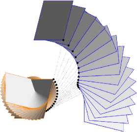
Figure 1: Two different motions with identical plane trajectory.

5 Conclusion and Future Research

We have presented a complete discussion of the problem to create a prescribed rational torse $[u]$ as plane trajectory of a rational motion. The torse necessarily needs to be kinematic, that is, have a possess a rational Gauss map. In general, if $\operatorname{realgcd}(\vec{u})=1$ the resulting motion of minimal degree is unique up to inessential coordinate transformations. Our constructive proofs allow to compute solutions of minimal degree and make effective use of the algebra of real and quaternionic polynomials. All solutions to the problem at hand are obtained by composing from the right a solution of minimal degree with rational planar motions that fix the moving plane.

A natural next question is to study the problem of creating a given rational ruled surface as trajectory of a straight line undergoing a rational motion. Again, there is the necessary condition on rationality of the ruled surface’s spherical image. Apart from that, little seems to be known. We expect, however, that techniques similar to the ones used by us in this article will provide a complete solution.

Once torses or ruled surfaces are described as plane or line trajectories of rational motions of low degree, motion factorization techniques can be used for the creation of mechanical linkages to “draw” them. It seems natural to adapt the techniques of [5, 6] to the case of plane and line trajectories, thus extending Kempe’s Universality Theorem to kinematic rational torses and to ruled surfaces. This is not an automatic task as one important insight of this article is that the rational motions to create a given line trajectory or a given plane trajectory have quite different characteristics.

The algebra of dual quaternions only allows to model the group $\operatorname{SE}(3)$ of rigid body displacements of Euclidean three-space. It might be a worthy undertaking to study similar problems in other algebras and kinematic spaces, for example the creation of one-parametric sets of circles by low degree motions in conformal kinematics. Possibly, this could unveil relations to rationally parametrized channel surfaces [20, 21].

We do believe that a thorough understanding of rational motions to create plane and line trajectories, its restrictions and its degrees of freedom, will ultimately also pave the way towards further application in engineering sciences.

A further and rather different line of research starts with the fundamental Equation (7) that we solved for an undetermined motion polynomial $C$ and a real polynomial $h$. It can be viewed as a generalization of Equation (8), an equation that describes the quaternionic pre-image of a polynomial Pythagorean-hodograph curve [17]. It can also be regarded as a special instance of an equation of Sylvester type. The Sylvester equation has been studied extensively in diverse algebraic context and in particular in the context of quaternionic function theory. However, in contrast to [22], we are not interested in “slice semi-regular quaternionic solution functions” to the general Sylvester equation $ax+xb=c$ but in low-degree polynomial solutions. We suggest the study of low degree polynomial solutions to Sylvester type equations in a general algebraic context might an interesting topic of future research.

References

- [1] I. I. Artobolevskii, Mechanisms for the generation of plane curves, Pergamon Press, Oxford, 1964.
- [2] M. G. Wagner, B. Ravani, Curves with rational frenet-serret motion, Computer Aided Geometric Design 15 (1) (1997) 79–101. doi:10.1016/s0167-8396(97)81786-4.
- [3] J. Prošková, Interpolations by rational motions using dual quaternions, Journal for Geometry and Graphics 21 (1) (2017) 71–78.
- [4] B. Jüttler, Über zwangläufige rationale Bewegungsvorgänge, Österreich. Akad. Wiss. Math.-Natur. Kl. S.-B. II 202 (1–10) (1993) 117–232.
- [5] M. Gallet, C. Koutschan, Z. Li, G. Regensburger, J. Schicho, N. Villamizar, Planar linkages following a prescribed motion, Mathematics of Computation 86 (303) (2016) 473–506. doi:10.1090/mcom/3120.
- [6] Z. Li, J. Schicho, H.-P. Schröcker, Kempe’s universality theorem for rational space curves, Found. Comput. Math. 18 (2) (2018) 509–536. doi:10.1007/s10208-017-9348-x.
- [7] O. Bottema, B. Roth, Theoretical Kinematics, Dover Publications, 1990.
- [8] J. M. Selig, Clifford algebra of points, lines and planes, Robotica 18 (5) (2000) 545–556. doi:10.1017/S0263574799002568.
- [9] R. Bodduluri, B. Ravani, Design of developable surfaces using duality between plane and point geometries, Comput. Aided Geom. Design 25 (1993) 621–632. doi:10.1016/0010-4485(93)90017-I.
- [10] Z. Li, J. Schicho, H.-P. Schröcker, The rational motion of minimal dual quaternion degree with prescribed trajectory, Comput. Aided Geom. Design 41 (2016) 1–9. doi:10.1016/j.cagd.2015.10.002.
- [11] G. Hegedüs, J. Schicho, H.-P. Schröcker, Factorization of rational curves in the Study quadric and revolute linkages, Mech. Maschine Theory 69 (1) (2013) 142–152. doi:10.1016/j.mechmachtheory.2013.05.010.
- [12] A. Damiano, G. Gentili, D. Struppa, Computations in the ring of quaternionic polynomials, Journal of Symbolic Computation 45 (1) (2010) 38–45. doi:10.1016/j.jsc.2009.06.003.
- [13] Z. Li, D. F. Scharler, H.-P. Schröcker, Factorization results for left polynomials in some associative real algebras: State of the art, applications, and open questions, J. Comput. Appl. Math. 349 (2019) 508–522. doi:10.1016/j.cam.2018.09.045.
- [14] M. I. Falcão, F. Miranda, R. Severino, M. J. Soares, Computational Science and Its Applications – ICCSA 2017, Springer International Publishing, 2017, Ch. Mathematica Tools for Quaternionic Polynomials, pp. 394–408. doi:10.1007/978-3-319-62395-5_27.
- [15] H. I. Choi, D. S. Lee, H. P. Moon, Clifford algebra, spin representation, and rational parameterization of curves and surfaces, Advances in Computational Mathematics 17 (1/2) (2002) 5–48. doi:10.1023/a:1015294029079.
- [16] H.-P. Schröcker, Z. Šír, Three paths to rational curves with rational arc length, Appl. Math. Comput. 478 (128842) (2024). doi:10.1016/j.amc.2024.128842.
- [17] R. Farouki, Pythagorean-Hodograph Curves: Algebra and Geometry Inseperable, Geometry and Computing, Springer, Berlin, Heidelberg, 2008.
- [18] C. C.-A. Cheng, T. Sakkalis, On new types of rational rotation-minimizing frame space curves, Journal of Symbolic Computation 74 (2016) 400–407. doi:10.1016/j.jsc.2015.08.005.
- [19] Z. Li, H.-P. Schröcker, D. F. Scharler, Motion polynomials admitting a factorization with linear factors, Accepted for publication in SIAM Journal on Applied Algebraic Geometry (2025). arXiv:2209.02306.
- [20] M. Peternell, H. Pottmann, Computing rational parametrizations of canal surfaces, Journal of Symbolic Computation 23 (2–3) (1997) 255–266. doi:10.1006/jsco.1996.0087.
- [21] G. Landsmann, J. Schicho, F. Winkler, The parametrization of canal surfaces and the decomposition of polynomials into a sum of two squares, Journal of Symbolic Computation 32 (1–2) (2001) 119–132. doi:10.1006/jsco.2001.0453.
- [22] A. Altavilla, C. de Fabritiis, Equivalence of slice semi-regular functions via sylvester operators, Linear Algebra and its Applications 607 (2020) 151–189. doi:10.1016/j.laa.2020.08.009.