A Generalized Numerical Framework for Improved Finite-Sized Key Rates with Rényi Entropy

Abstract

Quantum key distribution requires tight and reliable bounds on the secret key rate to ensure robust security. This is particularly so for the regime of finite block sizes, where the optimization of generalized Rényi entropic quantities is known to provide tighter bounds on the key rate. However, such an optimization is often non-trivial, and the non-monotonicity of the key rate in terms of the Rényi parameter demands additional optimization to determine the optimal Rényi parameter as a function of block sizes. In this work, we present a tight analytical bound on the Rényi entropy in terms of the Rényi divergence and derive the analytical gradient of the Rényi divergence. This enables us to generalize existing state-of-the-art numerical frameworks for the optimization of the key rate. With this generalized framework, we show improvements in regimes of high loss and low block sizes, which are particularly relevant for long-distance satellite-based protocols.

I Introduction

Quantum key distribution (QKD) is a cryptographic method for establishing secret keys between two distant parties, commonly called Alice and Bob, by exchanging quantum signals through a public quantum channel and using classical communication over an authenticated public channel [1, 2]. An adversary, referred to as Eve, can fully access the classical communication and potentially interfere with the quantum channel. Since the introduction of the first QKD protocol [1], QKD has evolved into various forms [3, 4, 5, 6] to enhance performance, simplify implementation, and address vulnerabilities.

A key performance metric for a QKD protocol is the secret key rate, defined as the ratio between the number of secret key bits and the number of raw quantum bits exchanged during the protocol. The secret key rate is determined by the full set of parameters governing the protocol such as noise and loss of the quantum channel, and assumptions on the attacking power of Eve. A central ingredient in formulating the key rate is the leftover hashing lemma [7, 8] which quantifies the number of secret bits distillable from privacy amplification requiring Eve has no knowledge of the final key. This quantification is expressed in terms of the smooth min-entropy which can be bounded by von Neumann entropy. The bound saturates in the asymptotic limit where the number of signals are infinite, due to the asymptotic equipartition property [9]. Early works  [10, 11] subsequently formally established the security for collective attacks and key rate formulas in the asymptotic regime. The security against general attacks are also established via the entropy accumulation theorem (EAT) [12, 13, 14, 15] and the postselection technique [16].

Since imperfections in sources and detectors in a practical QKD setup are inevitable, it quickly became evident that robust security proofs should be derived assuming that Eve may fully exploit such imperfections to her advantage [17, 18]. In essence, a practical QKD security proof necessitates further numerical optimizations based on the experimental parameters estimated by the honest parties. This optimization considers the worst-case scenario where Eve exploits device imperfections to perform an optimal attack. Winick et al. [19] developed a reliable numerical framework to evaluate the von Neumann key rate under collective attack through a two-step approach involving semi-definite programming (SDP). George et al. [20] subsequently extended the framework by incorporating finite size analysis, rendering it a highly valuable tool for evaluating the key rates of QKD implementations.

In a recent work by Dupuis  [21], it was shown that the key rate can be formulated directly in terms of the generalized Rényi entropies via a Rényi leftover hashing lemma. This new lemma eliminates the need for smoothing which is a challenging optimization problem over quantum states, and avoids loose bounds associated with the von Neumann entropy in the finite-size regime. By optimizing over a single Rényi parameter $\alpha$, this approach is expected to yield tighter bounds in the finite-size regime. Recent works [22, 23, 24, 25] have incorporated the Rényi leftover hashing lemma into key rate analysis. However, the bounds on the Rényi key rate remain loose, and numerical frameworks for the Rényi entropy key rate evaluations remain undeveloped due to the inherent challenges in optimizing the Rényi entropy.

In this work, we address these challenges by generalizing the numerical framework initially proposed by Winick et al. [19] to include the optimization of the generalized Rényi key rate. We derive a tight bound to the Rényi entropy in terms of the Rényi divergence and subsequently obtain an analytical expression for its gradient. These inputs are then utilized in the Frank-Wolfe algorithm [26] as part of the minimization algorithm. Additionally, we incorporate the finite-size framework originally introduced by George et al. [20] into our analysis for collective attacks and using the open-source numerical package (openQKDsecurity) [27]. Consequently, we achieve an improvement in key rate, which we demonstrate to be pertinent in practical scenarios, including in the presence of channel loss and noise.

This manuscript is organized as such: Section II provides the background of the basic QKD protocol framework, and Section III introduces the security proof formulation for Rényi entropy key rate. In Section IV we introduce our technical results and the formulation of the generalized framework. In Section V we conduct a numerical analysis using our generalized framework. Finally, Section VI concludes with a discussion and outlook for future work.

II QKD Protocol Framework

We begin by providing a brief overview of the basic QKD protocol framework and its mathematical formulations used for the security analysis. In particular, the source-replacement scheme provides an easy way to formulate prepare-and-measure protocols under the language of entanglement-based protocols [28, 29, 30]. Under this scheme, the prepare-and-measure protocol can be formulated as Alice preparing the state $|\Phi\rangle_{AA^{\prime}}$:

$$|\Phi\rangle_{AA^{\prime}}=\sum_{x}\sqrt{p_{x}}|x\rangle_{A}\otimes|\varphi_{x}\rangle_{A^{\prime}},$$ (1)

where $\{|x\rangle\}$ form an orthonormal basis, while Alice holds system $A$ and sends system $A^{\prime}$ to Bob. The action of a malicious eavesdropper Eve can be described by a quantum channel ${\cal E}:A^{\prime}\rightarrow B$ acting on the system $A^{\prime}$ before reaching Bob. The resulting state is $\rho_{AB}=({\cal I}_{A}\otimes{\cal E}_{A^{\prime}})(|\Phi\rangle\langle\Phi|_{AA^{\prime}})$. The basic framework for prepare and measure protocol under source-replacement can be summarized as follows:

1. For each round of the protocol $i\in\{0,1,\dots N\}$,

   1. State preparation and transmission: Alice prepares a bipartite state $|\Phi\rangle_{AA^{\prime}}$, keeps $A$ and sends $A^{\prime}$ to Bob. The system $A^{\prime}$ goes through a quantum channel before reaching Bob $B$.

   2. State measurement: Alice measures $A$ using a set of POVM and stores her measurement result in a classical register $X_{A}$. Bob measures $B$ using another set of POVM and stores his measurement result in a classical register $Y_{B}$. They subsequently store their choice of POVM in a public register.

   3. Public announcement: Alice and Bob exchange classical information from their public registers. The classical communication script is stored in a register $S$ for sifting.

   4. Sifting and key map: Alice and Bob either keep or discard their measurement results depending on $S$. The probability of the signal being kept is $p_{\textnormal{pass}}$. Alice subsequently applies a key map procedure on $A$ according to $X_{A}$ and maps into a classical raw key register $Z_{A}$.

2. Parameter estimation: Alice and Bob randomly choose a small proportion of measurement results $p_{\textnormal{test}}$ to construct a frequency distribution, which is used to estimate errors on the quantum channel. Such errors can be attributed to being caused by a malicious Eve with quantum side information $E^{\prime}$. The protocol is accepted if the frequency distribution falls within a set of previously agreed upon statistics, and is aborted otherwise; we denote this event as $\Omega_{\rm AT}$. The remaining number of signals for key generation is denoted as $n$, in other words $n=p_{\textnormal{pass}}p_{\textnormal{gen}}N$, where $p_{\textnormal{gen}}=1-p_{\textnormal{test}}$.

3. Error correction and verification: Alice and Bob exchange $\lambda_{EC}$ bits of information and store in a classical register $C$, so that Bob can perform error correction on his string and produce a guess of Alice’s key. To verify the correctness of this step, Alice sends a 2-universal hash of her key string of length $\log_{2}(1/\epsilon_{\textnormal{EV}})$ to Bob for error verification and is stored in another classical register $V$. Bob subsequently compares Alice’s hash with the hash of his guess. The protocol is accepted if the hash matches; we denote this event as $\Omega_{\rm EV}$, and $\epsilon_{\textnormal{EV}}$ as the failure probability of error verification.

4. Privacy amplification: Finally, Alice and Bob randomly pick a 2-universal hash function and apply it to their raw keys, producing the final secret keys $K_{A}$ and $K_{B}$ respectively. $\epsilon_{\textnormal{PA}}$ is denoted as the failure probability of privacy amplification.

Upon completion of the protocol, $\Pr[{\Omega_{\textnormal{acc}}}]=\Pr[{\Omega_{\textnormal{EV}}}\wedge{\Omega_{\textnormal{AT}}}]$ is the probability where the protocol is accepted ($\Pr[\bot]$ when aborted); in other words, ${\Omega_{\textnormal{acc}}}$ refers to the events where both parameter estimation and error verification succeed. To mathematically formulate the protocol, we denote the QKD protocol map ${\mathcal{M}}^{l}_{\textnormal{QKD}}\in{\cal C}(A^{n}B^{n},K_{A}K_{B}\tilde{C})$, where ${\cal C}$ is a CPTP map that maps $A^{n}B^{n}$ to $K_{A}K_{B}\tilde{C}$ and hashes to a key length $l$. Here, $\tilde{C}=S^{n}CV$ is the total public communication registers for $n$ rounds. Eve is assumed to hold the purification $\rho_{A^{n}B^{n}E^{\prime}_{n}}$ of the state $\rho_{A^{n}B^{n}}$. We also denote ${\mathcal{M}}^{l,\textnormal{ideal}}_{\textnormal{QKD}}$ as its idealized map. Then, we have that

$$( {\mathcal{M}}^{l}_{\textnormal{QKD}}\otimes\mathbb{I}_{E_{n}^{\prime}})(\rho_{A^{n}B^{n}E^{\prime}_{n}})$$ (2)

$$=\Pr({\Omega_{\textnormal{acc}}})\rho_{K_{A}K_{B}\tilde{C}E^{\prime}_{n}|{\Omega_{\textnormal{acc}}}}+\Pr(\bot)\rho^{\bot}_{K_{A}K_{B}\tilde{C}E^{\prime}_{n}},$$

$$( {\mathcal{M}}^{l,\textnormal{ideal}}_{\textnormal{QKD}}\otimes\mathbb{I}_{E_{n}^{\prime}})(\rho_{A^{n}B^{n}E^{\prime}_{n}})$$ (3)

$$=\Pr({\Omega_{\textnormal{acc}}})\bar{\rho}_{K_{A}K_{B}}\otimes\rho_{\tilde{C}E^{\prime}_{n}|{\Omega_{\textnormal{acc}}}}+\Pr(\bot)\rho^{\bot}_{K_{A}K_{B}\tilde{C}E^{\prime}_{n}},$$

where $\bar{\rho}_{K_{A}K_{B}}$ is a classical, perfectly correlated state with maximally mixed marginals. Since the output states when the protocol aborts are the same for both the real and ideal protocol maps [25], we have that

$$\left\lVert({\mathcal{M}}^{l}_{\textnormal{QKD}}-{\mathcal{M}}^{l,\textnormal{ideal}}_{\textnormal{QKD}})\otimes\mathbb{I}_{E_{n}^{\prime}}(\rho_{A^{n}B^{n}E^{\prime}_{n}})\right\rVert_{1}$$ (4)

$$=\Pr({\Omega_{\textnormal{acc}}})\left\lVert\rho_{K_{A}K_{B}\tilde{C}E^{\prime}_{n}|{\Omega_{\textnormal{acc}}}}-\bar{\rho}_{K_{A}K_{B}}\otimes\rho_{\tilde{C}E^{\prime}_{n}|{\Omega_{\textnormal{acc}}}}\right\rVert_{1}.$$

With this, we formally establish the security of the protocol via the following statement.

Definition II.1.

A QKD protocol is said to be $\epsilon$-secure if

$$\frac{1}{2}\left\lVert\left(({\mathcal{M}}^{l}_{\textnormal{QKD}}-{\mathcal{M}}^{l,\textnormal{ideal}}_{\textnormal{QKD}})\otimes\mathbb{I}_{E_{n}^{\prime}}\right)\rho_{A^{n}B^{n}E^{\prime}_{n}}\right\rVert_{1}\leq\epsilon.$$ (5)

Definition II.2.

Let ${\cal E}^{l}_{\textnormal{QKD}}=\operatorname{Tr}_{K_{B}}\circ{\mathcal{M}}^{l}_{\textnormal{QKD}}$ be a protocol map, and ${\cal E}^{l,\textnormal{ideal}}_{\textnormal{QKD}}$ be its idealized map. Given an $\epsilon$-secure QKD protocol, the protocol is said to be $\epsilon_{sec}$-secret if

$$\frac{1}{2}\left\lVert\left(({\cal E}^{l}_{\textnormal{QKD}}-{\cal E}_{\textnormal{QKD}}^{l,\textnormal{ideal}})\otimes\mathbb{I}_{E_{n}^{\prime}}\right)\rho_{A^{n}B^{n}E^{\prime}_{n}}\right\rVert_{1}\leq\epsilon_{\textnormal{sec}},$$ (6)

and $\epsilon_{corr}$-correct if

$$\Pr[K_{A}\neq K_{B}\wedge{\Omega_{\textnormal{acc}}}]\leq\epsilon_{\textnormal{corr}}.$$ (7)

where $\epsilon_{\textnormal{sec}}+\epsilon_{\textnormal{corr}}=\epsilon$.

III Security Proof with Rényi Entropy

An important element in our updated QKD security proof is the recently established leftover hashing lemma for Rényi entropies [21], which quantifies the amount of secret bits obtained from the 2-universal hash function during privacy amplification.

Theorem III.1.

Privacy Amplification ([21], Theorem 8). For $\alpha\in(1,2]$, we have $F:Z_{A}\rightarrow K_{A}$ as a family of two-universal hash function with $K_{A}=\{0,1\}^{l}$. If the hash function is drawn uniformly from $F$, then

$$\left\lVert\rho_{K_{A}EF}-\frac{\mathbb{I}_{K_{A}}}{|{\cal K}_{A}|}\otimes\rho_{EF}\right\rVert_{1}\leq 2^{g(l,\alpha,\rho)},$$ (8)

$$g(l,\alpha,\rho)=\frac{2}{\alpha}-1+\frac{1-\alpha}{\alpha}\left[H_{\alpha}(Z_{A}^{n}|\tilde{C}E^{\prime}_{n})_{\rho|{\Omega_{\textnormal{acc}}}}-l\right],$$

where $l=\log_{2}(|{\cal K}_{A}|)$ is the final length of the secret keys after hashing and $H_{\alpha}$ denotes the sandwiched conditional Rényi entropy.

A central technical quantity in Theorem III.1 is the conditional quantum Rényi entropy, which is defined as a special case of the sandwiched Rényi divergence.

Definition III.2.

(Sandwiched Rényi divergence and conditional entropy, [31]) For subnormalized quantum states $\rho,\sigma$ where $\mathop{\rm supp}\nolimits(\rho)\subseteq\mathop{\rm supp}\nolimits(\sigma)$, the sandwiched Rényi divergence $D_{\alpha}(\rho||\sigma)$ is defined for real values of $\alpha\in(0,\infty)$ as

$$D_{\alpha}(\rho||\sigma):=\frac{1}{\alpha-1}\log_{2}\frac{\left\lVert\sigma^{\frac{1-\alpha}{2\alpha}}\rho\sigma^{\frac{1-\alpha}{2\alpha}}\right\rVert_{\alpha}^{\alpha}}{\operatorname{Tr}(\rho)},$$ (9)

where $\lVert\rho\rVert_{p}=[\operatorname{Tr}(\rho^{p})]^{1/p}$ is the Schatten p-norm. For states $\rho_{AB}$, the conditional Rényi entropy for $\alpha\in(0,\infty)$ is

$$H_{\alpha}(A|B)_{\rho} :=-\inf_{\sigma_{B}}D_{\alpha}(\rho_{AB}||\mathbb{I}_{A}\otimes\sigma_{B}).$$ (10)

The conditional Rényi entropy is monotonically non-increasing in $\alpha$, and satisfies data processing inequality [32]. It also reduces to the von Neumann entropy at $\alpha\rightarrow 1$, and the conditional min-entropy when $\alpha\rightarrow\infty$. It thus recovers properly the conventional quantum entropic measures in a well-behaved manner, giving us a valuable information-theoretic measure to capture non i.i.d. (independent and identically distributed) features of general quantum states.

Following from Eq. 20 of Ref [24], the Rényi entropy can then be lower-bounded as shown

$$H_{\alpha}(Z^{n}_{A}|\tilde{C}E^{\prime}_{n})_{\rho|{\Omega_{\textnormal{acc}}}}\geq H_{\alpha}(Z_{A}^{n}|\tilde{C}E^{\prime}_{n})_{\rho|{\Omega_{\textnormal{AT}}}}-f(\alpha)$$ (11)

with a correction term $f(\alpha)=\frac{\alpha}{1-\alpha}\log_{2}\left(\Pr[{\Omega^{\prime}}]\right)$, where ${\Omega^{\prime}}={\Omega_{\textnormal{EV}}}|{\Omega_{\textnormal{AT}}}$ denotes the event of successful error verification, conditioned on the honest parties accepting parameter estimation. Subsequently, the Rényi entropy is further bounded by

$$H_{\alpha} (Z_{A}^{n}|\tilde{C}E^{\prime}_{n})_{\rho|{\Omega_{\textnormal{AT}}}}$$ (12)

$$\geq H_{\alpha}(Z_{A}^{n}|CS^{n}E^{\prime}_{n})_{\rho|{\Omega_{\textnormal{AT}}}}-\log_{2}\left(\frac{1}{\epsilon_{\textnormal{EV}}}\right).$$

[31] Since Eve also contains copies of the public announcements $S^{n}$, we denote her final system as $E_{n}=S^{n}E^{\prime}_{n}$. Finally, to account for key bits used for error correction, we show that the Rényi entropy decreases due to information leakage in the following lemma (see Appendix A for proof).

Lemma III.3.

(Decrease in Rényi entropy due to error correction) Given the Rényi entropy of Alice’s classical key $Z_{A}$ conditioned on error correction register $C$ and Eve’s total system $E$, the Rényi entropy can be related to the leakage term via the following:

$$H_{\alpha}(Z_{A}^{n}|CE_{n})\geq H_{\alpha}(Z_{A}^{n}|E_{n})-\lambda_{EC},$$ (13)

where $\lambda_{EC}=nf_{EC}H(Z_{A}|Y_{B})$ is the amount of bits leaked during public communication for error correction, and $f_{EC}$ is the error correction efficiency.

To formulate the security for the collective i.i.d. (independent and identically distributed) scenario, where Eve’s attack is i.i.d. for each round, i.e. $E_{n}=\rho_{E}^{\otimes n}=E^{n}$. As a result, similar to Eq. 21 of Ref [24], by using Theorem III.1 we have the following secrecy relation

$$\frac{1}{2} \left\lVert\left(\left({\cal E}^{l}_{\textnormal{QKD}}-{\cal E}_{\textnormal{QKD}}^{l,\textnormal{ideal}}\right)\otimes\mathbb{I}_{E_{n}^{\prime}}\right)\rho_{A^{n}B^{n}E^{\prime}_{n}}\right\rVert_{1}$$ (14)

$$\leq 2^{-\frac{\alpha-1}{\alpha}\left(\theta+2-l\right)}\leq\epsilon_{\textnormal{PA}},$$

where

$$\theta=nH_{\alpha}(Z_{A}|E)_{\rho|{\Omega_{\textnormal{AT}}}}-\log_{2}\left(\frac{1}{\epsilon_{\textnormal{EV}}}\right)-\lambda_{EC}.$$ (15)

Thus the final key length formula is

$$l\leq\theta+2-\frac{\alpha}{\alpha-1}\log_{2}\left(\frac{1}{\epsilon_{\textnormal{PA}}}\right).$$ (16)

IV A generalized numerical framework for key rates using Rényi entropies

In this section, we provide a generalization of the numerical framework in [19], which obtains the lower bound to the key rate via a two-step process. In the original framework, the von Neumann entropy is minimized to obtain a reliable lower bound to the key rate. The first step of the minimization is based on the Frank-Wolfe algorithm [26], as detailed in Algorithm 1. Here, $f(\rho)$ denotes the objective function to be optimized, and $\nabla f(\rho)$ is its gradient. In the second step for the minimization, a linearization is performed about the near-optimal state obtained from Step 1. The linearization is cast as a dual SDP problem to yield a lower bound to the key rate (see Appendix E).

1 Let $\epsilon>0,\rho_{0}\in\mathbf{S}$ and set $i=0$.

2 Compute $\Delta\rho:=\arg\min_{\Delta\rho}\operatorname{Tr}[(\Delta\rho)^{T}\nabla f(\rho_{i})]$ s.t. $\Delta\rho+\rho_{i}\in\mathbf{S}$.

3 If $\operatorname{Tr}[(\Delta\rho)^{T}\nabla f(\rho_{i})]<\epsilon$ then STOP.

4 Find $\lambda\in(0,1)$ that minimizes $f(\rho_{i}+\lambda\Delta\rho)$.

Set $\rho_{i+1}=\rho_{i}+\lambda\Delta\rho,i\leftarrow i+1$ and go to Step 2.

Algorithm 1 Step 1 Minimization [19]

We show that this framework can be generalized to optimize the Rényi entropy key rate in a similar fashion. To do so, one needs to first define the final state of the full protocol. This can be done by explicitly considering the postprocessing Kraus map ${\cal G}$, that models the state measurement, public announcements, and key map procedures of the protocol. It is formally described by ${\cal G}(\rho_{AB})=\sum_{s}p_{s}G_{s}\rho_{AB}G_{s}^{\dagger}$ [19]. Following from the simplified model in Ref [33] and as shown by Ref [34], $G_{s}$ can be expressed as

$$G_{s}=\sum_{x}|g(x,s)\rangle_{R}\otimes|x\rangle\!\langle x|_{A}\otimes\mathbb{I}_{B}\otimes|s\rangle_{S},$$ (17)

where ${\cal G}:AB\rightarrow RABS$. The function $g(x,s)$ maps the values $x$ and $s$ into a quantum register $R$. Alice then applies a key map isometry $V_{Z}$ to decohere $R$ and store the result in a classical register $Z_{A}$, resulting in a final classical-quantum state $\rho_{Z_{A}RABS}$. Without loss of generality, it is assumed that $\rho_{Z_{A}RABSE}$ is a purification of $\rho_{Z_{A}RABS}$. Next, we rewrite the Rényi entropy in terms of the Rényi divergence as shown in the following theorem.

Theorem IV.1.

Let $\rho_{Z_{A}RABS}=V_{Z}\rho_{RABS}V_{Z}^{\dagger}$ where $V_{Z}=\sum_{i}|i\rangle_{Z_{A}}\otimes Z^{i}_{R}$ and $Z_{R}^{i}$ is a rank-one $Z$ projector acting on $R$, and let $\rho_{Z_{A}RABSE}$ be its purification. Then, the sandwiched conditional Rényi entropy for $\alpha\in(1,2]$ can be expressed as

$$H_{\alpha}(Z_{A}|E) =\inf_{\sigma_{RABS}}D_{\beta}(\rho_{Z_{A}RABS}||\mathbb{I}_{Z_{A}}\otimes\sigma_{RABS})$$

$$=\inf_{\sigma_{AB}}D_{\beta}\bigl{(}{\cal G}(\rho_{AB})||{\cal Z}\circ{\cal G}(\sigma_{AB})\bigr{)}$$

$$=D_{\beta}\bigl{(}{\cal G}(\rho_{AB})\bigl{|}\bigr{|}{\cal Z}\circ{\cal G}(\rho_{AB})\bigr{)}.$$ (18)

Here, $\alpha,\beta$ are related via the duality relation $\frac{1}{\alpha}+\frac{1}{\beta}=2$, and ${\cal Z}(\cdot)=\sum_{i}(Z^{i}_{R}\otimes\mathbb{I}_{ABS})(\cdot)(Z^{i}_{R}\otimes\mathbb{I}_{ABS})$ is a pinching map, while $\mathcal{G}$ is the postprocessing map defined above with respect to the Kraus operators in Eq. (17).

The proof for Theorem IV.1 can be found in Appendix B. Theorem IV.1 is useful because it allows us to make use of the convexity of the sandwiched Rényi divergence for $\beta\in(0.5,1)$ and it also provides a tight bound to the Rényi entropy. The optimal key length is expressed as

$$l_{\textnormal{opt}} =\min_{\rho_{AB}\in\mathbf{S}}nD_{\beta}\Bigl{(}{\cal G}(\rho_{AB})\bigl{|}\bigr{|}{\cal Z}\circ{\cal G}(\rho_{AB})\Bigr{)}+2$$ (19)

$$-\frac{\alpha}{\alpha-1}\log_{2}\left(\frac{1}{\epsilon_{\textnormal{PA}}}\right)-\lambda_{EC}-\log_{2}\left(\frac{1}{\epsilon_{\textnormal{EV}}}\right).$$

The optimal key rate is expressed as the optimal key length divided by the total number of signals (rounds) sent, i.e. $r_{\textnormal{opt}}=l_{\textnormal{opt}}/N$. By noting that $p_{\textnormal{pass}}=\operatorname{Tr}({\cal G}(\rho_{AB}))$, the central quantity to be optimized can then be denoted as

$$f_{\beta}(\rho)=\operatorname{Tr}({\cal G}(\rho))\cdot D_{\beta}\Bigl{(}{\cal G}(\rho)\bigl{|}\bigr{|}{\cal Z}\circ{\cal G}(\rho)\Bigr{)}.$$ (20)

A key insight that allows for the simplification of our derivation, is that the state ${\cal G}(\rho_{AB})$ possesses additional structure under the pinching map ${\cal Z}$. In other words, one can show that for states $\rho_{AB}$ obtained via the source-replacement scheme,

$$[{\cal G}(\rho_{AB}),{\cal Z}\circ{\cal G}(\rho_{AB})]=0.$$ (21)

The proof of this statement is given in Appendix C. It makes use of the fact that $\mathcal{G}(\rho_{AB})=\rho_{RABS}$ has additional structure, if when Alice measures in $X$ or $Z$ basis, she obtains 0 or 1 with equal probability. Under this condition, the sandwiched Rényi divergence can be simplified as the Petz Rényi divergence [31]. This leads to our central analytical result, which is an expression of the gradient for Rényi divergence, and subsequently for our objective function $f_{\beta}(\rho)$.

Theorem IV.2.

For $[{\cal G}(\rho),{\cal Z}\circ{\cal G}(\rho)]=0$, the gradient of the objective function $f_{\beta}(\rho)$ is given by

$$\nabla f_{\beta}(\rho)= {\cal G}^{\dagger}\biggl{[}\mathbb{I}\cdot D_{\beta}\Bigl{(}{\cal G}(\rho)\bigl{|}\bigr{|}{\cal Z}\circ{\cal G}(\rho)\Bigr{)}\biggr{]}+$$ (22)

$$\biggl{.}\operatorname{Tr}\bigl{(}{\cal G}(\rho)\bigr{)}\cdot\nabla D_{\beta}\Bigl{(}{\cal G}(\rho)\bigl{|}\bigr{|}{\cal Z}\circ{\cal G}(\rho)\Bigr{)},$$

where the gradient of the Rényi divergence is given by

$$\nabla D_{\beta}\Bigl{(}{\cal G}(\rho)\bigl{|}\bigr{|}{\cal Z}\circ{\cal G}(\rho)\Bigr{)}$$ (23)

$$=\frac{1}{(\beta-1)}{\cal G}^{\dagger}\left[\frac{\chi_{1}+\chi_{2}}{Q_{\beta}({\cal G}(\rho)||{\cal Z}\circ{\cal G}(\rho))}-\frac{\mathbb{I}}{\operatorname{Tr}({\cal G}(\rho))}\right],$$

and

$$\chi_{1}=\beta{\cal G}(\rho)^{\beta-1}\bigl{(}{\cal Z}\circ{\cal G}(\rho)\bigr{)}^{1-\beta},$$

$$\chi_{2}=(1-\beta){\cal Z}\Bigl{(}{\cal G}(\rho)^{\beta}\bigl{(}{\cal Z}\circ{\cal G}(\rho)\bigr{)}^{-\beta}\Bigr{)},$$

$$Q_{\beta}(\rho\|\sigma)=\left\lVert\sigma^{\frac{1-\beta}{2\beta}}\rho\sigma^{\frac{1-\beta}{2\beta}}\right\rVert_{\beta}^{\beta}.$$ (24)

The proof of Thm. IV.2 is given in Appendix D. Taking L’Hôpital’s rule in the limit when $\beta\rightarrow 1$, we recover the objective function and gradient function as originally shown by Ref [19]:

$$\lim_{\beta\rightarrow 1}f_{\beta}(\rho) =D\Bigl{(}{\cal G}(\rho_{AB})\bigl{|}\bigr{|}{\cal Z}\circ{\cal G}(\rho_{AB})\Bigr{)},$$ (25)

$$\lim_{\beta\rightarrow 1}\nabla f_{\beta}(\rho) ={\cal G}^{\dagger}\Bigl{(}\log_{2}{\cal G}(\rho)-\log_{2}{\cal Z}\circ{\cal G}(\rho)\Bigr{)}.$$ (26)

Finally, to ensure continuity of the gradient function, the gradient is perturbed with a depolarizing channel ${\cal D}_{\epsilon}$, ${\cal G}_{\epsilon}(\rho)={\cal D}_{\epsilon}\circ{\cal G}(\rho)$ for $0<\epsilon<1$ [19]. TheoremIV.2 therefore provides us the keystone ingredient used in our generalized numerical framework.

V Numerical Analysis

In this section, we conduct a numerical security proof of the Rényi key rate using our generalized numerical framework. To account for finite-size in our numerical analysis, we incorporate the finite-size constraints by Ref [20] into our optimization problem (See Appendix E). Below is an analysis of the single photon BB84 protocol.

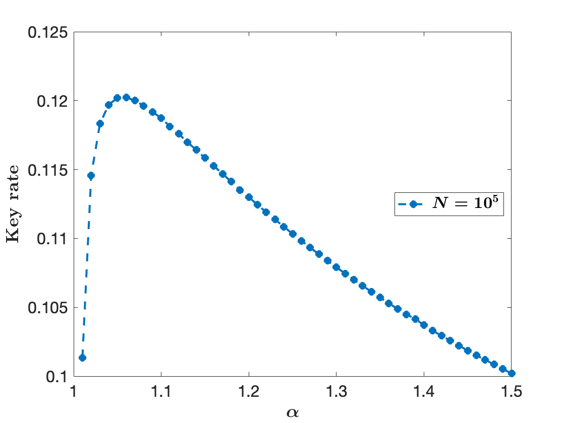
Figure 1: Numerical key rate at different values of $\alpha$ for $N=10^{5}$.

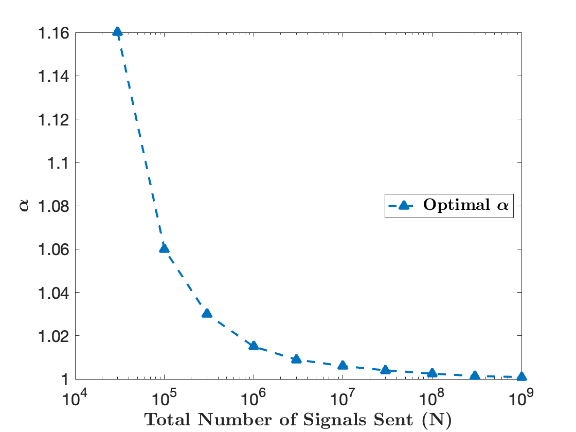
Figure 2: Optimal values of $\alpha$ for each signal block sizes $N$.

We begin by studying how the key rate varies with $\alpha$ (See Figure 1). The $\alpha$ dependency of the key length comes from the Rényi entropy term $H_{\alpha}(Z_{A}|E)$ as well as the factor of the $\log_{2}(1/(\epsilon_{PA}))$ term (See Eq (16)). These two terms are competing effects since the Rényi entropy is monotonically decreasing in $\alpha$ while the factor of the $\log_{2}$ term is increasing in $\alpha$. Hence, there exists an optimal $\alpha$ value for each signal block size $N$.

The optimal $\alpha$ for each signal block size is then determined and plotted as shown in Figure 2. From the figure, it can be seen that the optimal $\alpha$ values converge to 1 as $N$ approaches infinity, due to asymptotic equipartition property [9, 31]. By optimizing $\alpha$ for each block sizes, we show the advantage of the Rényi bounds obtained from our work compared to the original von Neumann bound proposed by Ref [20] in Figure 3. From Figure 3, it can be seen that the Rényi key rate yields a higher bound as compared to the von Neumann key rate in the low block size regime ($N<10^{7}$). This is especially evident for signal block size $N=10^{5}$, where the Rényi key rate doubles that of the von Neumann key rate. For $N\geq 10^{7}$, there is no significant difference between the two bounds.

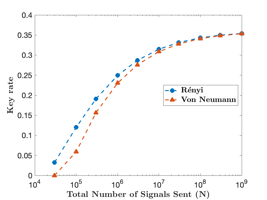
Figure 3: Rényi key rate computed at optimal $\alpha$ vs the von Neumann key rate with depolarizing probability $p=0.01$ and loss 0 dB.

When comparing against different values of loss, the Rényi entropy key rate also tends to outperform the von Neumann key rate in the high loss regime as seen in Figure 4. The Rényi entropy key rate is shown to be more tolerant towards loss since the von Neumann key rate decreases to zero more rapidly in the high loss regime.

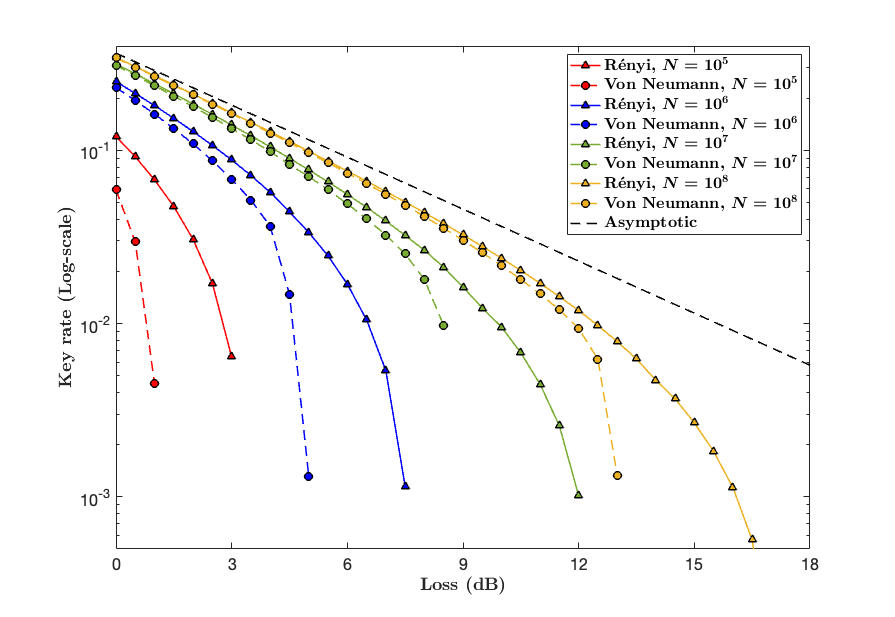
Figure 4: Key rate against channel loss with depolarizing probability $p=0.01$.

VI Discussion and Outlook

In this work, we have formulated the key rate in terms of the sandwiched Rényi entropy under collective attack and derived a tight bound on the sandwiched Rényi entropy using the Rényi divergence, and subsequently generalizes the numerical framework originally proposed by Ref [19]. Using this generalization, we computed the key rates for BB84 protocol. We also numerically computed the optimal values of $\alpha$ for each signal block size and showed that the optimal $\alpha$ approaches 1 when $N$ approaches infinity. An advantage of this generalization is the ability to optimize the Rényi entropy in a straightforward way. By bounding the Rényi entropy directly in terms of the Rényi divergence via the duality relation, we are able to obtain a tight lower-bound to the Rényi key rate as compared to previous works by Refs [25, 22] where the von Neumann entropy is used to relax the Rényi entropy analysis. As such, we are able to numerically compute an improved bound on the Rényi entropy key rate especially in the high loss regime. This improvement makes our generalized framework an important tool for the evaluation of long-range satellite-based QKD protocols, where signal block sizes remain small ($\sim 10^{5}$) with significant channel loss. Besides that, this generalization is versatile since it is also applicable to other protocols such as decoy state BB84 and measurement-device-independent (MDI) protocol.

A drawback of our method is the need for perturbing the gradient function to ensure a continuous gradient, leading to numerical imprecision. As such, the Facial Reduction method could be considered as an alternative. At the point of writing, we became aware of a separate and independent work on Rényi entropy key rate applied to decoy state QKD under coherent attacks [35]. It would be interesting to see how our framework could be applied to the study of other protocols such as the decoy state protocol under the coherent attack assumption.

Code Availability

The code used to obtain the data in this work can be found at https://github.com/Rebeccacrb07/openQKDsecurity.git.

SUPPLEMENTARY MATERIALS FOR “A GENERALIZED NUMERICAL FRAMEWORK FOR IMPROVED FINITE-SIZED KEY RATES WITH RÉNYI ENTROPY”

Appendix A Proof of Lemma III.3

In this section, we show how the Rényi entropy decreases under error correction. The proof follows with a simple calculation similar to Lemma 2 of Ref [41]:

$$H_{\alpha}(Z_{A}^{n}|E_{n}C) \geq H_{\alpha}(Z_{A}^{n}C|E_{n})-H_{\max}(C)$$ (27)

$$=H_{\alpha}(Z_{A}^{n}|E_{n})+H_{\alpha}(C|Z_{A}^{n})-H_{\max}(C)$$ (28)

$$\geq H_{\alpha}(Z_{A}^{n}|E_{n})+H_{\min}(C|Z_{A}^{n})-H_{\max}(C)$$ (29)

$$\geq H_{\alpha}(Z_{A}^{n}|E_{n})+H_{\min}(C|Z_{A}^{n}Y_{B}^{n})-H_{\max}(C)$$ (30)

$$\geq H_{\alpha}(Z_{A}^{n}|E_{n})-\lambda_{EC}.$$ (31)

The first inequality (27) proceeds from the chain rule for Rényi entropy given that $Z_{A}$ and $C$ are both classical variables (Equation 5.96 of Ref [31]). The first equality (28) is due to $C$ and $E_{n}$ being independent due to the Markov chain ($E_{n}\leftrightarrow Z_{A}^{n}\leftrightarrow C$) since the classical communication script $C$ is being computed by Alice and independent of Eve, hence $\rho_{Z_{A}^{n}C|E_{n}}=\rho_{Z_{A}^{n}|E_{n}}\otimes\rho_{C|Z_{A}^{n}}$ as shown in Ref [7]. The second inequality (29) follows from the monotonicity of the Rényi chain rule (Equation 5.73 of Ref [31]). The second inequality (30) is due to the decrease in the min-entropy upon conditioning. The final inequality (31) follows from Ref [41] where $\lambda_{EC}=nf_{EC}H(Z_{A}|Y_{B})$.

Appendix B Proof of Theorem IV.1

Here we prove that the Rényi entropy can be expressed in terms of the Rényi divergence via the duality relation, where $\frac{1}{\alpha}+\frac{1}{\beta}=2$. Let $\rho_{RABSE}$ be a purification of $\rho_{RABS}$. A key map isometry $V_{Z}=\sum_{i}|i\rangle_{Z_{A}}\otimes Z_{R}^{i}$ models the $Z$ projective measurement on $R$ and identity on all other systems, and subsequently stores the result in the classical register $Z_{A}$ [48]. We thus have $\rho_{Z_{A}RABS}=V_{Z}\rho_{RABS}V_{Z}^{\dagger}$ which is classical in $R$ and $Z_{A}$, and $\rho_{Z_{A}RABSE}$ as a purification of $\rho_{Z_{A}RABS}$ [48]. Then,

$$H_{\alpha}(Z_{A}|E) =-H_{\beta}(Z_{A}|RABS)$$ (32)

$$=\inf_{\sigma_{RABS}}D_{\beta}(\rho_{Z_{A}RABS}||\mathbb{I}_{Z_{A}}\otimes\sigma_{RABS})$$ (33)

$$\geq\inf_{\sigma_{RABS}}D_{\beta}(V_{Z}^{\dagger}\rho_{Z_{A}RABS}V_{Z}||V_{Z}^{\dagger}(\mathbb{I}_{Z_{A}}\otimes\sigma_{RABS})V_{Z})$$ (34)

$$=\inf_{\sigma_{RABS}}D_{\beta}(\rho_{RABS}||\sum_{i}Z_{R}^{i}(\sigma_{RABS})Z_{R}^{i})$$ (35)

$$=\inf_{\sigma_{AB}}D_{\beta}({\cal G}(\rho_{AB})||{\cal Z}\circ{\cal G}(\sigma_{AB}))$$ (36)

$$=D_{\beta}({\cal G}(\rho_{AB})||{\cal Z}\circ{\cal G}(\rho_{AB})).$$ (37)

The first equality stems from the duality relation of the Rényi entropy [32, 42, 49] for pure state $\rho_{Z_{A}RABSE}$. The inequality (34) is due to data-processing inequality, since $V_{Z}^{\dagger}$ is a partial isometry ($V_{Z}V_{Z}^{\dagger}\neq\mathbb{I}$). The final equality is due to the fact that ${\cal Z}\circ{\cal G}(\rho_{AB})$ attains the minimum (Theorem 2 of Refs [45, 44]).

$$H_{\alpha}(Z_{A}|E) =-H_{\beta}(Z_{A}|RABS)$$ (38)

$$\leq E_{R,\beta}^{Z_{A}|RABS}(\rho_{Z_{A}RABS})$$ (39)

$$=\inf_{\sigma\in\textnormal{sep}}D_{\beta}(\rho_{Z_{A}RABS}||\sigma_{Z_{A}RABS})$$ (40)

$$\leq D_{\beta}(V_{Z}\rho_{RABS}V_{Z}^{\dagger}||V_{Z}{\cal Z}(\rho_{RABS})V_{Z}^{\dagger})$$ (41)

$$=D_{\beta}({\cal G}(\rho_{AB})||{\cal Z}\circ{\cal G}(\rho_{AB})).$$ (42)

The first inequality is taken from Eq. (45) of Ref [49], where $E_{R,\beta}^{Z_{A}|RABS}$ is the Rényi relative entropy of entanglement between $Z_{A}$ and $RABS$. The second inequality is then obtained from the fact that $V_{Z}{\cal Z}(\rho_{RABS})V_{Z}^{\dagger}$ is a separable state as noted by Ref [48], since the system $R$ in ${\cal Z}(\rho_{RABS})$ is decohered in $Z$ due to the projective measurement. As noted in Ref [48], decoherence of a state occurs when a projective measurement is applied to a system’s reduced state, resulting in the loss of off-diagonal elements, therefore becoming a separable state. The final equality comes from the isometric invariance of the Rényi divergence as noted in Ref [31] ($V_{Z}^{\dagger}V_{Z}=\mathbb{I}$). From the above, $D_{\beta}({\cal G}(\rho_{AB})||{\cal Z}\circ{\cal G}(\rho_{AB}))\leq H_{\alpha}(Z_{A}|E)\leq D_{\beta}({\cal G}(\rho_{AB})||{\cal Z}\circ{\cal G}(\rho_{AB}))$, therefore all the above inequalities saturate and thus establishing Theorem IV.1.

Appendix C Proof of Proposition C.1

In this section, we show how the commutativity relation $[{\cal G}(\rho),{\cal Z}\circ{\cal G}(\rho)]=0$ holds under the source-replacement scheme.

Proposition C.1.

For states $\rho_{AB}$ obtained via the source-replacement scheme, and assuming that the probability of obtaining 0 or 1 upon measuring $A$ in either basis should be equal, we have

$$[{\cal G}(\rho_{AB}),{\cal Z}\circ{\cal G}(\rho_{AB})]=0.$$ (43)

Proof.

Under the source-replacement scheme, the state $\rho_{AB}$ is

$$\rho_{AB}=({\cal I}_{A}\otimes{\cal E}_{A^{\prime}\rightarrow B})(|\Phi\rangle\langle\Phi|_{AA^{\prime}}),$$ (44)

where $|\Phi\rangle_{AA^{\prime}}=\sum_{i}^{d}\sqrt{p_{i}}|i\rangle_{A}\otimes|\varphi_{i}\rangle_{A^{\prime}}$ where $d\in\mathbb{Z}^{+}$ is the dimension of Alice’s system. Here $p_{0},p_{1}$ corresponds to the probabilities of Alice preparing $|0\rangle$ and $|1\rangle$ respectively, while $p_{2},p_{3}$ corresponds to the probabilities of Alice preparing $|+\rangle$ and $|-\rangle$ respectively. By assumption of correctness of the protocol, we therefore have $p_{0}=p_{1}$ and $p_{2}=p_{3}$. For simplicity, we consider the basic qubit BB84 protocol, where the Kraus map is

$$G_{0} =\left(|0\rangle_{R}\otimes|0\rangle\!\langle 0|_{A}+|1\rangle_{R}\otimes|1\rangle\!\langle 1|_{A}\right)\otimes\mathbb{I}_{B}\otimes|0\rangle_{S},$$ (45)

$$G_{1} =\left(|0\rangle_{R}\otimes|2\rangle\!\langle 2|_{A}+|1\rangle_{R}\otimes|3\rangle\!\langle 3|_{A}\right)\otimes\mathbb{I}_{B}\otimes|1\rangle_{S}.$$ (46)

We first consider ${\cal G}_{0}(\rho)=G_{0}\rho G_{0}^{\dagger}$ for the $Z$-basis measurement on $A$. This yields the following

$${\cal G}_{0}(\rho_{AB}) =\sum_{i,j=0}^{1}|i\rangle\!\langle j|_{R}\otimes(|i\rangle\!\langle i|_{A}\otimes\mathbb{I}_{B})\rho_{AB}(|j\rangle\!\langle j|_{A}\otimes\mathbb{I}_{B})|0\rangle\!\langle 0|_{S}$$ (47)

$${\cal Z}\circ{\cal G}_{0}(\rho_{AB}) =\sum_{k=0}^{1}|k\rangle\!\langle k|_{R}\otimes(|k\rangle\!\langle k|_{A}\otimes\mathbb{I}_{B})\rho_{AB}(|k\rangle\!\langle k|_{A}\otimes\mathbb{I}_{B})\otimes|0\rangle\!\langle 0|_{S}.$$ (48)

Hence, we obtain the following relation

$$\bigl{(}{\cal Z}\circ{\cal G}_{0}(\rho_{AB})\bigr{)}\cdot{\cal G}_{0}(\rho_{AB}) =\sum_{i,j,k=0}^{1}|k\rangle\delta_{ik}\langle j|_{R}\otimes(|k\rangle\!\langle k|_{A}\otimes\mathbb{I}_{B})\rho_{AB}(|k\rangle\delta_{ik}\langle i|_{A}\otimes\mathbb{I}_{B})\rho_{AB}(|j\rangle\!\langle j|_{A}\otimes\mathbb{I}_{B})\otimes|0\rangle\!\langle 0|_{S}$$ (49)

$$=\sum_{i,j=0}^{1}|i\rangle\!\langle j|_{R}\otimes(|i\rangle\!\langle i|_{A}\otimes\mathbb{I}_{B})\rho_{AB}(|i\rangle\!\langle i|_{A}\otimes\mathbb{I}_{B})\rho_{AB}(|j\rangle\!\langle j|_{A}\otimes\mathbb{I}_{B})\otimes|0\rangle\!\langle 0|_{S},$$ (50)

$${\cal G}_{0}(\rho_{AB})\cdot\bigl{(}{\cal Z}\circ{\cal G}_{0}(\rho_{AB})\bigr{)} =\sum_{i,j,k=0}^{1}|i\rangle\delta_{jk}\langle k|_{R}\otimes(|i\rangle\!\langle i|_{A}\otimes\mathbb{I}_{B})\rho_{AB}(|j\rangle\delta_{jk}\langle k|_{A}\otimes\mathbb{I}_{B})\rho_{AB}(|k\rangle\!\langle k|_{A}\otimes\mathbb{I}_{B})\otimes|0\rangle\!\langle 0|_{S}$$ (51)

$$=\sum_{i,j=0}^{1}|i\rangle\!\langle j|_{R}\otimes(|i\rangle\!\langle i|_{A}\otimes\mathbb{I}_{B})\rho_{AB}(|j\rangle\!\langle j|_{A}\otimes\mathbb{I}_{B})\rho_{AB}(|j\rangle\!\langle j|_{A}\otimes\mathbb{I}_{B})\otimes|0\rangle\!\langle 0|_{S}.$$ (52)

From the above, we can see that to satisfy the commutativity relation, we must have

$$(|i\rangle\!\langle i|_{A}\otimes\mathbb{I}_{B})\rho_{AB}(|i\rangle\!\langle i|_{A}\otimes\mathbb{I}_{B})\rho_{AB}(|j\rangle\!\langle j|_{A}\otimes\mathbb{I}_{B})=(|i\rangle\!\langle i|_{A}\otimes\mathbb{I}_{B})\rho_{AB}(|j\rangle\!\langle j|_{A}\otimes\mathbb{I}_{B})\rho_{AB}(|j\rangle\!\langle j|_{A}\otimes\mathbb{I}_{B})$$ (53)

The LHS can be further simplified to

$$|i\rangle\!\langle i|\rho_{A}|i\rangle\!\langle i|\rho_{A}|j\rangle\!\langle j|=|i\rangle\rho_{A}^{ii}\rho_{A}^{ij}\langle j|,$$ (54)

and the RHS to

$$|i\rangle\!\langle i|\rho_{A}|j\rangle\!\langle j|\rho_{A}|j\rangle\!\langle j| =|i\rangle\rho_{A}^{ij}\rho_{A}^{jj}\langle j|.$$ (55)

For this to satisfy the commutativity relation, Eqs. (54) and (55) have to be equal. Given that $p_{i}=p_{j}=p$, this must hold true, meaning that the diagonal elements of Alice’s system $\rho_{A}^{ii}=\rho_{A}^{jj}=p$ are equal. Repeating the above derivation for the $X$ basis yields the full proof. ∎

Appendix D Proof of Theorem IV.2

Finally, we give the proof to the gradient of the sandwiched Rényi divergence as defined in Def. III.2. To begin, we first use the following shorthand $Q_{\beta}$:

$$Q_{\beta}(\rho||\sigma)=\left\lVert\sigma^{\frac{1-\beta}{2\beta}}\rho\sigma^{\frac{1-\beta}{2\beta}}\right\rVert_{\beta}^{\beta}=\operatorname{Tr}\left(\sigma^{\frac{1-\beta}{2\beta}}\rho\sigma^{\frac{1-\beta}{2\beta}}\right)^{\beta}$$ (56)

such that we have $D_{\beta}(\rho||\sigma)\equiv\frac{1}{\beta-1}\log_{2}\left(\frac{Q_{\beta}(\rho||\sigma)}{\operatorname{Tr}(\rho)}\right)$. We next need to show the derivative of this function $Q_{\beta}({\cal G}(\rho)||{\cal Z}\circ{\cal G}(\rho))$, for states obtained from the application of ${\cal G}$ and ${\cal Z}\circ{\cal G}$. Here, it is convenient to make use of Proposition C.1 to note that such states would always commute. In particular, for states $\rho,\sigma$ that commute with each other, we know that $Q_{\beta}$ can be rewritten as

$$Q_{\beta}(\rho\|\sigma)={\rm Tr}(\rho^{\beta}\sigma^{1-\beta}).$$ (57)

This form of $Q_{\beta}$ simplifies the calculation of its derivative, $\partial_{x}Q_{\beta}(\rho\|\sigma)$, which is the goal of the technical lemma below.

Lemma D.1.

Consider a state $\rho$ such that $[{\cal G}(\rho),{\cal Z}\circ{\cal G}(\rho)]=0$. Then, given a parametrization $\rho_{x}\equiv(1-x)\rho+x\tau$ with a scalar $x$, we first denote

$$Q_{\beta}({\cal G}(\rho_{x} )||{\cal Z}\circ{\cal G}(\rho_{x}))=\operatorname{Tr}({\cal G}(\rho_{x})^{\beta}\cdot{\cal Z}\circ{\cal G}(\rho_{x})^{1-\beta}).$$ (58)

Then we have that the derivative of $Q_{\beta}({\cal G}(\rho_{x})||{\cal Z}\circ{\cal G}(\rho_{x}))$ with respect to $x$ reads as

$$\partial_{x}Q_{\beta}({\cal G}(\rho_{x})||{\cal Z}\circ{\cal G}(\rho_{x}))=\operatorname{Tr}[(\tau-\rho)\cdot{\cal G}^{\dagger}\left(\chi_{1x}+\chi_{2x}\right)],$$ (59)

where ${\cal G}^{\dagger}(\cdot)=\sum_{i}p_{i}G_{i}^{\dagger}(\cdot)G_{i}$, and

$$\chi_{1x} =\beta{\cal G}(\rho_{x})^{\beta-1}{\cal Z}\circ{\cal G}(\rho_{x})^{1-\beta},$$ (60)

$$\chi_{2x} =(1-\beta){\cal Z}\left({\cal G}(\rho_{x})^{\beta}\cdot{\cal Z}\circ{\cal G}(\rho_{x})^{-\beta}\right).$$ (61)

Proof.

Noting that derivative and trace commute, we rewrite Eq. (59) using the product rule $\partial(X\cdot Y)=(\partial X)\cdot Y+X\cdot(\partial Y)$

$$\partial_{x}\operatorname{Tr}({\cal G}(\rho_{x})^{\beta}\cdot{\cal Z}\circ{\cal G}(\rho_{x})^{1-\beta})=\operatorname{Tr}[\partial_{x}({\cal G}(\rho_{x})^{\beta})\cdot{\cal Z}\circ{\cal G}(\rho_{x})^{1-\beta}+{\cal G}(\rho_{x})^{\beta}\cdot\partial_{x}({\cal Z}\circ{\cal G}(\rho_{x})^{1-\beta})].$$ (62)

Next, from Lemma 1 of Ref [47], we see that

$$\partial_{x}(\rho_{x}^{\beta})=\frac{\sin(\pi\beta)}{\pi}\int_{0}^{\infty}\frac{\tau-\rho}{(\rho_{x}+t)^{2}}t^{\beta}dt.$$ (63)

Using this for $\partial_{x}({\cal G}(\rho_{x})^{\beta})$ and $\partial_{x}({\cal Z}\circ{\cal G}(\rho_{x})^{1-\beta})$, while noting that $\mathcal{G}$ is linear yields

$$\partial_{x}({\cal G}(\rho_{x})^{\beta}) =\frac{\sin(\pi\beta)}{\pi}\int_{0}^{\infty}\frac{{\cal G}(\tau-\rho)}{({\cal G}(\rho_{x})+t)^{2}}t^{\beta}dt,$$ (64)

$$\partial_{x}({\cal G}\circ{\cal Z}(\rho_{x})^{1-\beta}) =\frac{\sin(\pi(1-\beta))}{\pi}\int_{0}^{\infty}\frac{{\cal Z}\circ{\cal G}(\tau-\rho)}{({\cal Z}\circ{\cal G}(\rho_{x})+t)^{2}}t^{1-\beta}dt.$$ (65)

Given that $[{\cal G}(\rho),{\cal Z}\circ{\cal G}(\rho)]=0$, and using the relation

$$\int_{0}^{\infty}\frac{1}{(A+t)^{2}}t^{k}dt=\frac{A^{k-1}}{\textnormal{sinc}(\pi k)},\qquad\text{for all }k\in(-1,0)\cup(0,1),$$ (66)

where $\textnormal{sinc}(x)=\frac{\sin(x)}{x}$, Eq. (62) then becomes

$$\partial_{x} \operatorname{Tr}({\cal G}(\rho_{x})^{\beta}\cdot{\cal Z}\circ{\cal G}(\rho_{x})^{1-\beta})$$ (67)

$$= \operatorname{Tr}\left[{\cal G}(\tau-\rho)\cdot\beta{\cal G}(\rho_{x})^{\beta-1}{\cal Z}\circ{\cal G}(\rho_{x})^{1-\beta}\right]+\operatorname{Tr}\left[{\cal Z}\circ{\cal G}(\tau-\rho)\cdot(1-\beta){\cal G}(\rho_{x})^{\beta}{\cal Z}\circ{\cal G}(\rho_{x})^{-\beta}\right].$$ (68)

Using the cyclic property of the trace, the first trace term on the RHS of Eq. (68) can be rewritten as

$$\operatorname{Tr} \left[\sum_{i}p_{i}G_{i}(\tau-\rho)G_{i}^{\dagger}\cdot\beta{\cal G}(\rho_{x})^{\beta-1}{\cal Z}\circ{\cal G}(\rho_{x})^{1-\beta}\right]$$ (69)

$$= \operatorname{Tr}\left[(\tau-\rho)\sum_{i}p_{i}G_{i}^{\dagger}\Bigl{(}\beta{\cal G}(\rho_{x})^{\beta-1}{\cal Z}\circ{\cal G}(\rho_{x})^{1-\beta}\Bigr{)}G_{i}\right]$$ (70)

$$= \operatorname{Tr}\biggl{[}(\tau-\rho)\cdot{\cal G}^{\dagger}\Bigl{(}\beta{\cal G}(\rho_{x})^{\beta-1}{\cal Z}\circ{\cal G}(\rho_{x})^{1-\beta}\Bigr{)}\biggr{]}.$$ (71)

which gives us Eq. (60). Doing the same for the second term in Eq. (68) yields the desired form for (61). This concludes our proof for Lemma D.1. ∎

Theorem D.2.

For states ${\cal G}(\rho)$ and ${\cal Z}\circ{\cal G}(\rho)$, the gradient of the Rényi divergence is given by

$$\nabla D_{\beta}\Bigl{(}{\cal G}(\rho)\bigl{|}\bigr{|}{\cal Z}\circ{\cal G}(\rho)\Bigr{)}=\frac{1}{(\beta-1)}{\cal G}^{\dagger}\left[\frac{\chi_{1}+\chi_{2}}{Q_{\beta}({\cal G}(\rho)||{\cal Z}\circ{\cal G}(\rho))}-\frac{\mathbb{I}}{\operatorname{Tr}({\cal G}(\rho))}\right],$$ (72)

with

$$\chi_{1}=\beta{\cal G}(\rho)^{\beta-1}\bigl{(}{\cal Z}\circ{\cal G}(\rho)\bigr{)}^{1-\beta},$$

$$\chi_{2}=(1-\beta){\cal Z}\Bigl{(}{\cal G}(\rho)^{\beta}\bigl{(}{\cal Z}\circ{\cal G}(\rho)\bigr{)}^{-\beta}\Bigr{)}.$$

Proof.

To begin, we introduce the Fréchet’s derivative (Sec. V.3 and Sec. X.4 of Ref [46]) of the Rényi divergence in the direction of $\tau$ at a point $\rho$ as

$$\partial_{\tau}D_{\beta}({\cal G}(\rho)\|{\cal Z}\circ{\cal G}(\rho)) \left.\equiv\partial_{x}D_{\beta}\bigl{(}{\cal G}(\rho_{x})\|{\cal Z}\circ{\cal G}\left(\rho_{x}\right)\bigr{)}\right|_{x=0}$$ (73)

$$\equiv\operatorname{Tr}[(\tau-\rho)\nabla D_{\beta}({\cal G}(\rho)\|{\cal Z}\circ{\cal G}(\rho))],$$ (74)

where we have denoted $\rho_{x}\equiv(1-x)\rho+x\tau$ as the state $\rho$ being parameterized with a scalar $x$, with $\partial_{\tau}=\frac{\partial}{\partial\tau}$ and $\partial_{x}=\frac{\partial}{\partial x}$. The derivative of $D_{\beta}({\cal G}(\rho_{x})||{\cal Z}\circ{\cal G}(\rho_{x}))$ with respect to $x$ is

$$\partial_{x}D_{\beta}({\cal G}(\rho_{x})||{\cal Z}\circ{\cal G}(\rho_{x}))=\frac{1}{\beta-1}\frac{\operatorname{Tr}({\cal G}(\rho_{x}))}{Q_{\beta}({\cal G}(\rho_{x})||{\cal Z}\circ{\cal G}(\rho_{x}))}\partial_{x}\left(\frac{Q_{\beta}({\cal G}(\rho_{x})||{\cal Z}\circ{\cal G}(\rho_{x}))}{\operatorname{Tr}({\cal G}(\rho_{x}))}\right).$$ (75)

Applying the quotient rule allows us to rewrite Eq. (75) as

$$\partial_{x}D_{\beta}({\cal G}(\rho_{x})||{\cal Z}\circ{\cal G}(\rho_{x}))=\frac{1}{\beta-1}\left[\frac{\partial_{x}Q_{\beta}({\cal G}(\rho_{x})||{\cal Z}\circ{\cal G}(\rho_{x}))}{Q_{\beta}({\cal G}(\rho_{x})||{\cal Z}\circ{\cal G}(\rho_{x}))}-\frac{\partial_{x}\operatorname{Tr}({\cal G}(\rho_{x}))}{\operatorname{Tr}({\cal G}(\rho_{x}))}\right].$$ (76)

By substituting Lemma D.1 into Eq. (76), and using the fact that $\partial_{x}\operatorname{Tr}({\cal G}(\rho_{x}))=\operatorname{Tr}[(\tau-\rho)\cdot{\cal G}^{\dagger}(\mathbb{I})]$ gives

$$\partial_{x}D_{\beta}\left({\cal G}(\rho_{x})\|{\cal Z}\circ{\cal G}\left(\rho_{x}\right)\right),$$ (77)

$$=\operatorname{Tr}\left[(\tau-\rho)\cdot\frac{1}{\beta-1}{\cal G}^{\dagger}\left(\frac{\chi_{1x}+\chi_{2x}}{Q_{\beta}\left({\cal G}(\rho_{x})\|{\cal Z}\circ{\cal G}\left(\rho_{x}\right)\right)}-\frac{\mathbb{I}}{\operatorname{Tr}({\cal G}(\rho_{x}))}\right)\right].$$

Taking $x=0$ gives

$$\left.\partial_{x}D_{\beta}\left({\cal G}(\rho_{x})\|{\cal Z}\circ{\cal G}\left(\rho_{x}\right)\right)\right|_{x=0}\equiv\operatorname{Tr}\left[(\tau-\rho)\cdot\nabla D_{\beta}({\cal G}(\rho)\|{\cal Z}\circ{\cal G}(\rho_{x}))\right].$$ (78)

This concludes our proof for Theorem D.2. ∎

Finally, we are in the position to prove Theorem IV.2. Given that $f_{\beta}(\rho)=\operatorname{Tr}({\cal G}(\rho))\cdot D_{\beta}\bigl{(}{\cal G}(\rho)\|{\cal Z}\circ{\cal G}(\rho)\bigr{)}$, using product rule and Eq. (78), we have

$$\partial_{x}f_{\beta}(\rho_{x})|_{x=0}= \left.\partial_{x}\Bigl{(}\operatorname{Tr}[{\cal G}(\rho_{x})]\Bigr{)}\cdot D_{\beta}\left({\cal G}(\rho_{x})\|{\cal Z}\circ{\cal G}\left(\rho_{x}\right)\right)\right|_{x=0}+\operatorname{Tr}[{\cal G}(\rho_{x})]\cdot\left.\partial_{x}\Bigl{(}D_{\beta}\left({\cal G}(\rho_{x})\|{\cal Z}\circ{\cal G}\left(\rho_{x}\right)\right)\Bigr{)}\right|_{x=0}$$ (79)

$$= \operatorname{Tr}[(\tau-\rho){\cal G}^{\dagger}(\mathbb{I})]\cdot D_{\beta}({\cal G}(\rho)||{\cal Z}\circ{\cal G}(\rho))+\operatorname{Tr}[{\cal G}(\rho)]\cdot\operatorname{Tr}\bigl{[}(\tau-\rho)\cdot\nabla D_{\beta}({\cal G}(\rho)\|{\cal Z}\circ{\cal G}(\rho))\bigr{]}.$$

We then use the fact that $D_{\beta}({\cal G}(\rho)\|{\cal Z}\circ{\cal G}\left(\rho\right))$ and $\operatorname{Tr}[{\cal G}(\rho)]$ are scalars, hence

$$\operatorname{Tr}\bigl{[}(\tau-\rho){\cal G}^{\dagger}(\mathbb{I})\bigr{]}\cdot D_{\beta}({\cal G}(\rho)\|{\cal Z}\circ{\cal G}\left(\rho\right)) =\operatorname{Tr}\Bigl{\{}(\tau-\rho){\cal G}^{\dagger}\bigl{[}\mathbb{I}\cdot D_{\beta}({\cal G}(\rho)\|{\cal Z}\circ{\cal G}\left(\rho\right))\bigr{]}\Bigr{\}}$$ (80)

$$\operatorname{Tr}[{\cal G}(\rho)]\cdot\operatorname{Tr}\bigl{[}(\tau-\rho)\cdot\nabla D_{\beta}({\cal G}(\rho)\|{\cal Z}\circ{\cal G}\left(\rho\right))\bigr{]} =\operatorname{Tr}\bigl{[}(\tau-\rho)\operatorname{Tr}[{\cal G}(\rho)]\cdot\nabla D_{\beta}({\cal G}(\rho)\|{\cal Z}\circ{\cal G}\left(\rho\right))\bigr{]}.$$ (81)

This gives us the resulting relation

$$\partial_{x}f_{\beta}(\rho_{x})|_{x=0} =\operatorname{Tr}\biggl{\{}(\tau-\rho)\Bigl{[}{\cal G}^{\dagger}\bigl{[}\mathbb{I}\cdot D_{\beta}({\cal G}(\rho)\|{\cal Z}\circ{\cal G}\left(\rho\right))\bigr{]}+\operatorname{Tr}[{\cal G}(\rho)]\cdot\nabla D_{\beta}({\cal G}(\rho)\|{\cal Z}\circ{\cal G}\left(\rho\right))\Bigr{]}\biggr{\}}$$ (82)

$$\equiv\operatorname{Tr}\bigl{[}(\tau-\rho)\nabla f_{\beta}(\rho)\bigr{]}.$$ (83)

This concludes our proof for Theorem IV.2.

Appendix E SDP Formulation with Finite-Size Constraints

In this section we introduce the finite-size constraints used for the optimization of the key rate. Following from Ref [20], the set of density matrices over which the optimization is performed for the prepare and measure protocol is

$$\mathbf{S_{\textnormal{PM}}}= \{\rho\in{\cal D}({\cal H}_{A}\otimes{\cal H}_{B})|\quad\exists F\in\mathcal{P}(\Sigma)$$ (84)

$$\textnormal{such that}\quad\operatorname{Tr}(\Gamma_{i}\rho)=\gamma_{i}\quad,\quad\forall i\in|\Sigma|$$

$$\quad\quad\quad\quad\quad\lVert\Phi_{\mathcal{P}}(\rho)-F\rVert_{1}\leq\mu$$

$$\quad\quad\quad\quad\quad\lVert F-\bar{F}\rVert_{1}\leq t\},$$

where $\mathcal{P}(\Sigma)$ is the probability distribution of size $\Sigma$. The first equality constraint takes into account Alice’s certainty of her state, where $\Gamma_{i}=M_{A}^{i}\otimes\mathbb{I}_{B}$. The second inequality constraint models the parameter estimation step, where only the set of states that are a $\mu$ distance away from the agreed frequency $F$ is accepted. The map $\Phi_{\mathcal{P}}(\rho)=\sum_{i}\operatorname{Tr}(\rho\tilde{\Gamma})_{i}|i\rangle\!\langle i|$, where $\tilde{\Gamma}_{i}=M_{A}^{i}\otimes M_{B}^{i}$ maps $\rho$ into a probability distribution of the measurement outcome by Alice and Bob. In this work, we consider the protocol with unique acceptance, hence we have $t=0\Rightarrow F=\bar{F}$.

Upon completion of the first step of the minimization, a close-to-optimal state $\hat{\rho}$ is obtained and subsequently linearized such that the optimal point $f(\rho^{*})$ is lower bounded by the following (Eqns. 77-79 of Ref [19])

$$f(\rho^{*}) \geq f(\hat{\rho})+\operatorname{Tr}((\rho^{*}-\hat{\rho})^{T}\nabla f(\hat{\rho}))$$ (85)

$$\geq f(\hat{\rho})-\operatorname{Tr}(\hat{\rho}^{T}\nabla f(\hat{\rho}))+\min_{\sigma\in\mathbf{S_{\textnormal{PM}}}}\operatorname{Tr}(\sigma^{T}\nabla f(\hat{\rho})).$$ (86)

Eq. (86) together with  (84) can be cast as an SDP problem to yield a primal problem.

$$\min \langle\nabla f(\rho),\sigma\rangle$$ (87)

s.t. $$\operatorname{Tr}\left(\Gamma_{i}\sigma\right)=\gamma_{i}\quad\forall i\in\Sigma,$$

$$\operatorname{Tr}\left(A\right)+\operatorname{Tr}\left(B\right)\leqslant\mu,$$

$$A\succeq\Phi_{\mathcal{P}}(\sigma)-\bar{F},$$

$$B\succeq-\left[\Phi_{\mathcal{P}}(\sigma)-\bar{F}\right]$$

$$\sigma,A,B\geq 0.$$

The corresponding dual problem is

$$\max \vec{\gamma}\cdot\vec{y}+\bar{f}\cdot\bar{z}-a\mu$$ (88)

s.t. $$\sum_{i}y_{i}\Gamma_{i}+\sum_{j}z_{j}\tilde{\Gamma}_{j}\leq f(\rho)$$

$$-a\mathbb{I}\leq\vec{z}\leq a\mathbb{I}$$

$$a\geq 0,\vec{y}\in\mathbb{R}^{|\Sigma|},$$

where $\bar{f}$ is the vector version of $\bar{F}$.

References

- Bennett and Brassard [2014] C. H. Bennett and G. Brassard, Quantum cryptography: Public key distribution and coin tossing, Theoretical Computer Science 560, 7 (2014), theoretical Aspects of Quantum Cryptography – celebrating 30 years of BB84.
- Ekert [1991] A. K. Ekert, Quantum cryptography based on bell’s theorem, Physical review letters 67, 661 (1991).
- Wolf [2021] R. Wolf, Quantum key distribution, Lecture notes in physics 988 (2021).
- Diamanti et al. [2016] E. Diamanti, H.-K. Lo, B. Qi, and Z. Yuan, Practical challenges in quantum key distribution, npj Quantum Information 2, 1 (2016).
- Xu et al. [2020] F. Xu, X. Ma, Q. Zhang, H.-K. Lo, and J.-W. Pan, Secure quantum key distribution with realistic devices, Reviews of modern physics 92, 025002 (2020).
- Pirandola et al. [2020] S. Pirandola, U. L. Andersen, L. Banchi, M. Berta, D. Bunandar, R. Colbeck, D. Englund, T. Gehring, C. Lupo, C. Ottaviani, et al., Advances in quantum cryptography, Advances in optics and photonics 12, 1012 (2020).
- Renner [2008] R. Renner, Security of quantum key distribution, International Journal of Quantum Information 6, 1 (2008).
- Tomamichel et al. [2011] M. Tomamichel, C. Schaffner, A. Smith, and R. Renner, Leftover hashing against quantum side information, IEEE Transactions on Information Theory 57, 5524 (2011).
- Tomamichel [2012] M. Tomamichel, A framework for non-asymptotic quantum information theory, arXiv preprint arXiv:1203.2142 (2012).
- Devetak and Winter [2005] I. Devetak and A. Winter, Distillation of secret key and entanglement from quantum states, Proceedings of the Royal Society A: Mathematical, Physical and engineering sciences 461, 207 (2005).
- Berta et al. [2010] M. Berta, M. Christandl, R. Colbeck, J. M. Renes, and R. Renner, The uncertainty principle in the presence of quantum memory, Nature Physics 6, 659 (2010).
- Dupuis et al. [2020] F. Dupuis, O. Fawzi, and R. Renner, Entropy accumulation, Communications in Mathematical Physics 379, 867 (2020).
- George et al. [2022] I. George, J. Lin, T. van Himbeeck, K. Fang, and N. Lütkenhaus, Finite-key analysis of quantum key distribution with characterized devices using entropy accumulation, arXiv preprint arXiv:2203.06554 (2022).
- Metger and Renner [2023] T. Metger and R. Renner, Security of quantum key distribution from generalised entropy accumulation, Nature Communications 14, 5272 (2023).
- Metger et al. [2024] T. Metger, O. Fawzi, D. Sutter, and R. Renner, Generalised entropy accumulation, Communications in Mathematical Physics 405, 261 (2024).
- Christandl et al. [2009] M. Christandl, R. König, and R. Renner, Postselection technique for quantum channels with applications to quantum cryptography, Physical review letters 102, 020504 (2009).
- Gottesman et al. [2004] D. Gottesman, H.-K. Lo, N. Lutkenhaus, and J. Preskill, Security of quantum key distribution with imperfect devices, in International Symposium on Information Theory, 2004. ISIT 2004. Proceedings. (2004) p. 136.
- Scarani et al. [2009] V. Scarani, H. Bechmann-Pasquinucci, N. J. Cerf, M. Dušek, N. Lütkenhaus, and M. Peev, The security of practical quantum key distribution, Reviews of modern physics 81, 1301 (2009).
- Winick et al. [2018] A. Winick, N. Lütkenhaus, and P. J. Coles, Reliable numerical key rates for quantum key distribution, Quantum 2, 77 (2018).
- George et al. [2021] I. George, J. Lin, and N. Lütkenhaus, Numerical calculations of the finite key rate for general quantum key distribution protocols, Physical Review Research 3, 013274 (2021).
- Dupuis [2023] F. Dupuis, Privacy amplification and decoupling without smoothing, IEEE Transactions on Information Theory (2023).
- Tupkary et al. [2024] D. Tupkary, E. Y.-Z. Tan, and N. Lütkenhaus, Security proof for variable-length quantum key distribution, Physical Review Research 6, 023002 (2024).
- Arqand et al. [2024] A. Arqand, T. A. Hahn, and E. Y.-Z. Tan, Generalized Rényi entropy accumulation theorem and generalized quantum probability estimation, arXiv preprint arXiv:2405.05912 (2024).
- Kamin et al. [2024] L. Kamin, A. Arqand, I. George, N. Lütkenhaus, and E. Y.-Z. Tan, Finite-size analysis of prepare-and-measure and decoy-state qkd via entropy accumulation, arXiv preprint arXiv:2406.10198 (2024).
- Nahar et al. [2024] S. Nahar, D. Tupkary, Y. Zhao, N. Lütkenhaus, and E. Y.-Z. Tan, Postselection technique for optical quantum key distribution with improved de finetti reductions, PRX Quantum 5, 040315 (2024).
- Frank et al. [1956] M. Frank, P. Wolfe, et al., An algorithm for quadratic programming, Naval research logistics quarterly 3, 95 (1956).
- Burniston et al. [2024] J. Burniston, W. Wang, L. Kamin, et al., Open QKD Security: Version 2.0.2, https://github.com/Optical-Quantum-Communication-Theory/openQKDsecurity (2024).
- Bennett et al. [1992] C. H. Bennett, G. Brassard, and N. D. Mermin, Quantum cryptography without bell’s theorem, Physical review letters 68, 557 (1992).
- Curty et al. [2004] M. Curty, M. Lewenstein, and N. Lütkenhaus, Entanglement as a precondition for secure quantum key distribution, Physical review letters 92, 217903 (2004).
- Ferenczi and Lütkenhaus [2012] A. Ferenczi and N. Lütkenhaus, Symmetries in quantum key distribution and the connection between optimal attacks and optimal cloning, Physical Review A—Atomic, Molecular, and Optical Physics 85, 052310 (2012).
- Tomamichel [2015] M. Tomamichel, Quantum information processing with finite resources: mathematical foundations, Vol. 5 (Springer, 2015).
- Beigi [2013] S. Beigi, Sandwiched Rényi divergence satisfies data processing inequality, Journal of Mathematical Physics 54 (2013).
- Lin et al. [2019] J. Lin, T. Upadhyaya, and N. Lütkenhaus, Asymptotic security analysis of discrete-modulated continuous-variable quantum key distribution, Physical Review X 9, 041064 (2019).
- Kamin and Lütkenhaus [2024] L. Kamin and N. Lütkenhaus, Improved decoy-state and flag-state squashing methods, Physical Review Research 6, 043223 (2024).
- Kamin et al. [2025] L. Kamin, J. Burniston, N. Lütkenhaus, and E. Y.-Z. Tan, Rényi security framework against coherent attacks applied to decoy-state QKD (2025), in preparation.
- Wootters and Zurek [1982] W. K. Wootters and W. H. Zurek, A single quantum cannot be cloned, Nature 299, 802 (1982).
- Wang and Lütkenhaus [2022] W. Wang and N. Lütkenhaus, Numerical security proof for the decoy-state bb84 protocol and measurement-device-independent quantum key distribution resistant against large basis misalignment, Physical Review Research 4, 043097 (2022).
- Tan [2021] E. Y.-Z. Tan, Prospects for device-independent quantum key distribution, arXiv preprint arXiv:2111.11769 (2021).
- Arnon-Friedman and Renner [2015] R. Arnon-Friedman and R. Renner, de finetti reductions for correlations, Journal of Mathematical Physics 56 (2015).
- Fawzi and Renner [2015] O. Fawzi and R. Renner, Quantum conditional mutual information and approximate markov chains, Communications in Mathematical Physics 340, 575 (2015).
- Scarani and Renner [2008] V. Scarani and R. Renner, Security bounds for quantum cryptography with finite resources, in Workshop on Quantum Computation, Communication, and Cryptography (Springer, 2008) pp. 83–95.
- Müller-Lennert et al. [2013] M. Müller-Lennert, F. Dupuis, O. Szehr, S. Fehr, and M. Tomamichel, On quantum Rényi entropies: A new generalization and some properties, Journal of Mathematical Physics 54 (2013).
- Modi et al. [2012] K. Modi, A. Brodutch, H. Cable, T. Paterek, and V. Vedral, The classical-quantum boundary for correlations: Discord and related measures, Reviews of Modern Physics 84, 1655 (2012).
- Luo and Fu [2010] S. Luo and S. Fu, Geometric measure of quantum discord, Physical Review A—Atomic, Molecular, and Optical Physics 82, 034302 (2010).
- Modi et al. [2010] K. Modi, T. Paterek, W. Son, V. Vedral, and M. Williamson, Relative entropy of quantum and classical correlations, Phys. Rev. Lett 104, 080501 (2010).
- Bhatia [2013] R. Bhatia, Matrix analysis, Vol. 169 (Springer Science & Business Media, 2013).
- Rubboli and Tomamichel [2024] R. Rubboli and M. Tomamichel, New additivity properties of the relative entropy of entanglement and its generalizations, Communications in Mathematical Physics 405, 162 (2024).
- Coles [2012] P. J. Coles, Unification of different views of decoherence and discord, Physical Review A—Atomic, Molecular, and Optical Physics 85, 042103 (2012).
- Zhu et al. [2017] H. Zhu, M. Hayashi, and L. Chen, Coherence and entanglement measures based on Rényi relative entropies, Journal of Physics A: Mathematical and Theoretical 50, 475303 (2017).