Impact of phase signal formulations on tilt-to-length coupling noise in the LISA test mass interferometer

Abstract

TTL coupling in the Laser Interferometer Space Antenna (LISA) can generate spurious displacement noise that potentially affects the measurement of gravitational wave signals. In each test mass interferometer, the coupling of misalignments with spacecraft angular jitter produces noise in the longitudinal pathlength signal. This signal comes from the phase readout combinations of an interfering measurement beam and a local reference beam at a quadrant photodetector, but various formulations exist for its calculation. Selection of this pathlength signal formulation affects the tilt-to-length (TTL) coupling noise. We therefore simulated two pathlength signal candidates, the complex sum and the averaged phase, and evaluated their performance in the LISA test mass interferometer under the assumption of static alignment imperfections. All simulations were performed using three different methods with cross-checked results. We find with all three methods that the averaged phase is the choice with equal or less TTL coupling noise in four out of the five test cases. Finally, we show that the non-linear TTL contributions in the test mass interferometer to be negligible in all our test-cases, no matter which formulation of pathlength signal is chosen.

Keywords: tilt-to-length coupling, pathlength signal, laser interferometry, space interferometer, gravitational waves, LISA instrumentation

1 Introduction

The Laser Interferometer Space Antenna (LISA) is a gravitational wave detector that was recently adopted by ESA with an anticipated launch in the mid-2030s [1]. The primary objective of LISA is to observe the gravitational wave spectrum in the millihertz band, a range that is currently inaccessible to ground-based detectors [2]. This band is richly populated by compact binary systems in which the characteristic strain is $\mathcal{O}(10^{-21})$. LISA will consist of a triangular constellation of three identical spacecraft, each featuring two movable optical sub-assemblies that point along the line-of-sight to the other two remote spacecraft. Each sub-assembly houses a telescope and an optical bench with several interferometers for science and reference measurements. Each spacecraft is equipped with two gravitational reference systems (GRSs), comprising the hardware and avionics necessary to hold, release, and maintain the respective test masses in free-fall. A specialized electrode housing within a gravitational reference system (GRS), which features capacitive position sensing capabilities, encloses a single free-falling Au-Pt alloy test mass, monitoring. This monitors any displacement of the test mass from its center.

To enable length measurements between three pairs of test masses, six one-way laser links will be established between the spacecraft. The test mass-to-test mass differential length fluctuations generated by gravitational waves - and by certain noise sources - will be measured at each optical bench via the heterodyne beats of a measurement beam (MB) with a reference beam, termed the local oscillator (LO), which enters from the adjacent optical bench of the spacecraft. For technical reasons, the test mass-to-test mass link is split into three individual measurements. The first is the inter-satellite interferometer (ISI), which measures the distance between a link’s optical benches forming the endpoints of the inter-spacecraft distance. The other two measurements are at the test mass interferometers (TMIs) of linked spacecraft, which measures displacement of each test mass with respect to the local OB. The test mass interferometer (TMI), which is the focus of this work, is sketched in Fig. 1 below.

Figure 1: A condensed sketch of the test mass interferometer. Upon reflection from the test mass, the measurement beam is combined with the local oscillator at a beamsplitter before passing through an imaging system and being detected at a quadrant photodetector.

By utilizing post-processing techniques and combining interferometer readouts, LISA will achieve its required $\textrm{pm}/\sqrt{\textrm{Hz}}$ displacement sensitivity over the mission bandwidth. The feasibility of this pm-scale sensitivity has been partly proven by the LISA Pathfinder (LPF) mission [3]. However, several noise sources inherent to LISA’s interferometers remain to be investigated. For one, the interferometric detectors are vulnerable to spurious displacement fluctuations, e.g. due to spacecraft angular jitters. This leakage of angular motion into the pathlength signal is known as TTL coupling, and was already shown to be a significant noise source in LPF [4].

There are numerous publications on TTL coupling summarized, for example, in [5]. However, only one of these has considerable overlap with the content presented here. Of all the publications on TTL coupling, a recent paper ([6]) by members of the Taiji community, has the closest connection to ours with a study of the TTL noise in the TMI. However, that paper discusses the optimization of the design of an imaging system and its placement for the suppression of first and second order geometric TTL within the TMI of the Taiji mission, as well as in-orbit calibration. Likewise, results in [7, 8] consider cross-coupling from lateral jitter of the test mass (TM). Meanwhile, our study is focused on investigating various static misalignments coupled with spacecraft-to-test mass angular jitter at the interferometric quadrant photodiode (QPD) level, effectively maintaining a black box view of the imaging optics. In particular, we demonstrate in this paper that the way in which the longitudinal pathlength signal (LPS) itself is defined can serve to preemptively mitigate TTL noise caused by certain misalignments. This arises from the fact that the QPD utilized in the TMI generates four distinct pathlength signals, each corresponding to a detector quadrant. Although several definitions have been proposed to combine these four signals into a unified pathlength readout [9, 10], no definitive selection has been made for the TMI yet. So, a key question in optimizing readout remains: which pathlength definition is least affected by TTL contributions?

To investigate pathlength formulations and identify patterns in signals generated by particular noise sources, we have systematically probed a parameter space of misalignments which would generate TTL noise in the TMI readout. These misalignments can be inherited by the MB and LO at the QPD, so we simulated interference of the misaligned beams and computed their beat signals. We then used these signals to compare the readout fidelity of two specific longitudinal pathlength formulations - averaged phase (LPSA) and complex sum (LPSC) - for their use at the TMI. The remainder of the paper reports this simulation and is structured as follows:

• Section 2 provides an overview of TTL coupling in the TMI and a full description of our simulation parameter space.

• Section 3 contains a summary of the three simulation methods and a derivation of the interferometric signal formulations.

• Section 4 is focused on results of the two signal formulations and the effectiveness of eliminating the TTL coupling by subtracting the linear fit model from the two signal formulations.

• Finally, Section 5 concludes with implications of the results and outlines future work involving TTL noise simulation for the ISI.

2 Simulation at the test mass interferometer

In this section, we explore potential sources of pathlength readout noise in the TMI. We introduce a simplified simulation environment that distills an otherwise complex setup, including the imaging system, to its fundamental components and focuses on testable parameters related to TTL noise. From there, we outline the parameter space of our simulations.

2.1 The imaging system and tilt-to-length coupling

Each TMI comprises a free-falling test mass in an electrode housing, several optics, and a QPD. Additionally, a Gaussian MB propagates through components on the optical bench, to the test mass, then finally to the QPD where it combines with a Gaussian LO. However, in its path from the test mass reflective surface, as in Fig. 1, the MB acquires pathlength fluctuations with respect to the reference LO due to relative spacecraft-to-test mass angular jitter.

Imaging optics mitigate these fluctuations by reorienting each beam’s final center of rotation (CoR) - ideally, to the center of the QPD. Ultimately, the true success of the imaging system lies in its cancellation of the phase offset present between the LO and the misaligned MB on their combination at the QPD. This phase rectification capability can be described most simply with a single, combined lens, as in Fig. 2 below.

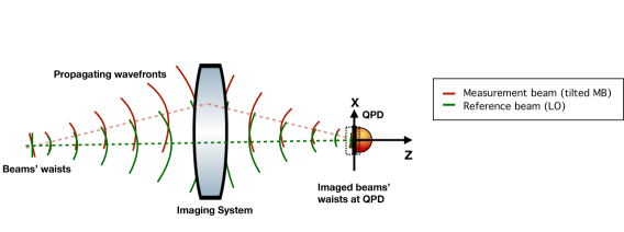
Figure 2: This simplified sketch of the imaging system depicts: a single lens; a measurement beam (the dashed optical axis in red); a local oscillator (the dashed optical axis in green); and a photodiode, which has a detector surface centered at the origin of the axes. The propagating wavefronts are imaged to ensure their phase offset, which otherwise introduces a spurious pathlength signal, is cancelled on combination at the detector.

2.2 Simplification of the simulation environment

Assuming perfect imaging without abberation, the imaging system can most easily be incorporated into simulation by considering its geometric effect on beam angles and sizes. Firstly, the imaging system (IS) alters the beam angle from $\alpha$ before the IS, to $(\alpha^{\prime})$ after the IS, and both angles relate by the magnification factor $m$:

$$\alpha^{\prime}=m\cdot\alpha\;,$$ (1)

and we define both angles relative to the QPD normal (cf.Fig. 3).

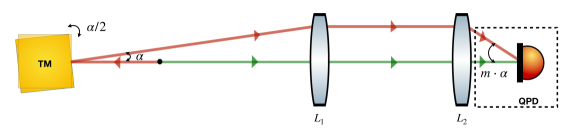
Figure 3: A sketch of the condensed test mass interferometer, where spacecraft-to-test mass relative jitter yields a beam tilt $\alpha$ in the MB (red) relative to the LO (green). After passing the imaging system, shown here with two lenses, the MB is redirected onto the QPD at an angle, but it is recentered at the QPD.

Meanwhile, the incident beam waist ($w_{0}$) is scaled to the emergent beam waist ($w_{0}^{\prime}$) by the magnification as

$$w_{0}^{\prime}=\frac{w_{0}}{m}\;.$$ (2)

Here, we assume that the waists are located in the pupil planes of the IS. Ideally, the IS then images a center of rotation which is located along the beam axis prior to the imaging system, onto the center of the QPD. The geometric effect observable on the QPD is given by a simple scaling of the incident beams and a rotation of the MB about the QPD center. Under these circumstances, the imaging optics suppress all geometric TTL coupling. Nevertheless, non-geometric effects can cause residual TTL noise to arise, e.g., from mismatches of the interfering wavefront curvatures. This can be mitigated by matching the beam properties, such that the two beam waists share an identical size and location on the QPD surface. In such a case, the non-geometric TTL also vanishes, as shown in [11] and illustrated in Fig. 2.

In our simulation, the goal was to consider the dominant TTL noise sources upstream along the TMI, before beam combination, and condense them into a simple model. The TMI is a complex system of optics and other components which are not necessary to implement in a full TTL simulation. Instead, pathlength signals are more simply derived from a combined parameter space of perturbations that we consider to be inherited by the MB and LO in their final relative geometries at the QPD. Therefore, a more simple simulation environment is one which includes only the dashed box portion of Fig. 3 - that is, the misaligned combining beams and the QPD. This is the testbed used in our simulation.

By this simplification, we must propagate all misalignments through the beam geometries such that angular jitter is translated into beam misalignments or offsets with respect to the nominal optical axes. However, if we consider the dominant sources of misalignment to be the test mass and IS, as in Fig. 3, we need only to incorporate their geometric effects into the parameter space to simulate practical interferometric signals.

2.3 Simulation setup

Due to the described simplification, we assume a condensed setup to describe the key features of the TMI. The setup features are nominally:

• The MB and LO have the same beam properties, i.e., equal waist sizes and Rayleigh ranges ($z_{\textrm{R}}$).

• The waists of the MB and LO are scaled down with the magnification of the imaging system ($m=2.5$).

• For the non-rotated case of the MB, the MB and LO have identical beam axes, which impinge at normal incidence onto the center of the QPD. The waist locations and the MB’s center of rotation nominally lie at the center of the QPD representing the case of ideal imaging.

• The simulated jitter of the MB is twice the expected jitter of the test mass relative to the spacecraft (see Fig. 3). Additionally, this doubled angle is further magnified by the imaging system, such that the total beam jitter on the QPD is five times that of the spacecraft-to-test mass angular jitter.

• The waist size of each beam is set to a conservative value ($\sim 400\,\upmu$m) such that it fits sufficiently on the $1\,$mm-width QPD active area.

Based on the assumptions outlined above, we consider an ideal scenario characterized by the absence of both geometric and non-geometric TTL coupling (see Figs. 3 and 2). In the context of this study, we analyze the impact of coupling on two signal formulations. We specifically focus on deviations from this ideal case, which we generically term misalignments.

2.4 Beam, photodiode, and misalignment parameters

The previous section described the nominal settings. We now describe the imperfections and variations to these nominal settings that we consider as outlined by Table 1. The nominal values here represent the zero TTL case of ideal alignment of the MB and LO along the optical axis. These are listed in the second column. The third column shows the ranges for which we tested the TTL coupling caused by variations of the listed parameters, and the fourth column shows the subsection in which the corresponding test is described.

Table 1: Nominal and test values for parameters used in simulation.

Parameter	Nominal Value	Test Values	Subsections
Wavelength $\lambda$ (both beams)	1064 nm	-	-
Circular Photodiode Diameter	1 mm	-	2.4.1
Square Photodiode Width	{$\sqrt{2}$/2, 1} mm	-	2.4.1
Photodiode Gap	20 $\upmu$m	-	2.4.1
Beam Tilts ($\alpha$)	0 $\upmu$rad	[-900, 900] $\upmu$rad	2.4.2
Waist radius ($w_{0}$)	402 $\upmu$m	{362,382,402,422,442} $\upmu$m	2.4.3, 4.1
Beam Lateral Offset ($x_{\textrm{off}}$)	$0\,$mm	$\pm\{0,0.1,0.2\}\,$mm	2.4.4, 4.2
Beam Lateral CoR ($x_{\textrm{cor}}$)	0 mm	$\pm\{0,0.5,1\}$ mm	2.4.5, 4.3
Beam Waist Longitudinal Offset ($z_{\textrm{off}}$)	0 mm	$\pm\{0,23.8,47.6\}$ mm	2.4.6, 4.4
Beam Longitudinal CoR ($z_{\textrm{cor}}$)	0 mm	$\pm\{0,2.5,5\}$ mm	2.4.7, 4.5

Note that small changes in both the longitudinal and lateral positions of the beams and CoR could significantly increase the noise [8]. For example, in reality, the CoR of the spacecraft (or the MB) is some arbitrary point that yields a longitudinal and lateral offset at the entrance pupil of the lens system. Similarly, some errors are expected in the position of the beams. The following subsections illustrate the simulation parameters and further describe their selection criteria under this consideration.

2.4.1 Photodiode dimensions

In LISA, we expect circular quadrant photodiodes to be used and assume for the dimensions of these a diameter of $1\,$ mm and a gap width of $20\,\upmu$m [2, 12, 13]. However, circular geometry can be implemented in only one of the three simulation methods used in this paper. For this reason, we also tested square QPDs, which can be used with all three methods. To test the effect of the square shape, we implemented two different sizes for these square QPDs: “small” $\sqrt{2}/2\,$mm-width squares, which are inscribed within the circular QPD, and “large” 1 mm-width square which are circumscribed around the circular QPDs. These settings are sketched in Fig. 4a.

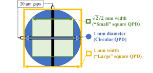
(a)

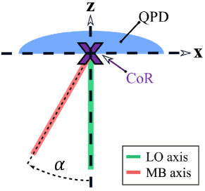
(b)

Figure 4: (a) shows overlays of the 1 mm-diameter circular (blue), $\sqrt{2}/2\,$mm “small” square (green), and 1 mm “large” square (yellow) QPDs used in simulation. In all test cases, inactive gaps between quadrants were 20 $\upmu$m (not to scale here). (b) shows the simplest misalignment case - MB (red) rotation by angle $\alpha$ about the QPD center (purple “X”), with an on-axis LO (green) and no other parameter variations.

2.4.2 Beam tilt

The “default” geometry of beam tilt ($\alpha$) with no other misalignment is shown in Fig. 4b. Note that the LO (shown in green) is optimally aligned along the interferometric $z$-axis, and the only variation to the MB (shown in red) is a rotation around the $y$-axis and about the QPD’s center. For this setup, we tested how much the beam could be tilted before the interferometric contrast vanishes. Additionally, we tested the linearity of the DWS signal over the same range.

The range of angles for this rotation is shown in Fig. 5 in units of the beam divergence angle, $\theta$ (i.e., we plot $\alpha/\theta$), where

$$\theta=\arctan\left(\frac{\lambda}{\pi w_{0}}\right)=842\,\upmu\textrm{rad}.$$ (3)

From Fig. 5 we found for all tested QPD shapes and sizes that the differential wavefront sensing signal (DWS) signal, which is a photodetector phase readout scheme used to track angular alignment, is approximately linear within a beam tilt range of at least $\alpha=\pm 1\cdot\theta$. Within this range, the interferometer has more than 60% contrast, which is high enough to ensure quality of all readout signals. We rounded the tilt range up to $\pm 900\,\upmu$rad and used this for all of our test cases.

[] []

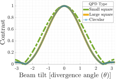
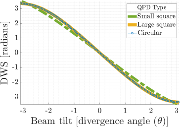
Figure 5: (a) Contrast and (b) DWS signals calculations for the three QPD sizes simulated: $\sqrt{2}/2\,$mm “small” square (dashed green), 1 mm “large” square (yellow), and 1 mm-diameter circular (blue) QPDs. Values on the $x$-axis are in units of divergence angle ($\theta=840$ $\upmu$rad) for tilt of one of the two beams.

2.4.3 Beam size

The laser itself and the waist sizes of the MB and LO are part of the ongoing LISA design [14]. The nominal value of $w_{0}=402\,\upmu$m for waist radii was chosen not only as a rough match to the expected mission parameters, but also because it represents the optimal fitting and good overlap of a Gaussian beam with a $900\,\upmu$m tophat beam diameter (a value we have used for ongoing simulation of tophat-Gaussian interference at the ISI). Table 1 shows that we have varied this waist radius for either of the beams at a time by up to $\pm 10\%$, and tested its effect on the TTL coupling. Physically, change to a single waist size term manifests as imperfect mode matching at the QPD. The $\pm 10\%$ variation was chosen from an order of magnitude estimate of how well the spot sizes can be matched on the optical bench. Our results of the waist size variations performed are shown in Section 4.1.

2.4.4 Lateral offset of the MB

In this first scenario of misalignment coupled with beam tilt, the MB is laterally offset ($x_{\textrm{off}}$) along the $x$-axis before the rotation about the $y$-axis described in Section 2.4.2. The value was set to be $0.2\,$mm, which represents one-half of the Gaussian beam radius. This magnitude of lateral beam shift is significantly higher than what we expect for LISA. However, this range allowed comfortable modeling of the TTL coupling, while maintaining functional contrast (here $c>0.5$). This type of lateral misalignment of the MB could originate from tolerances during the assembling of the optics prior to the imaging system. The simulation results are discussed in Section 4.2.

2.4.5 Lateral shift of the MB’s CoR

The beam tilts investigated within this paper can originate from either spacecraft or test mass angular jitter. Ideally, the pivot of both these jitters would laterally coincide with the center of the test mass. The imaging system then projects this pivot onto the QPD center.

We now consider cases where the MB does not pivot around the QPD center, but around a point laterally shifted by up to $x=1\,$mm. This could originate from a laterally shifted pivot of the test mass or spacecraft jitter. Alternatively, this could be caused by non-ideal imaging, or by both (a non-ideal pivot location and imperfect imaging) at the same time. An offset of $1\,$mm at the QPD translates to a displacement of the jitter pivot point by $2.5\,$mm, which we estimate to be a reasonable to optimistic value for spacecraft jitter but an exaggerated case for the test mass.

Please note that in the case of a lateral displacement of the center of rotation of the spacecraft or test mass, additional geometric TTL effects would occur, which we do not consider in this study. However, here we focus solely on the TTL due to the described lateral displacement at the QPD level. Our simulation results for this test are shown in Section 4.3.

2.4.6 Longitudinal offset of the waist

Longitudinal offset ($z_{\textrm{off}}$) repesents a defocus caused by mode mismatch. This value was varied within a range of $\pm 47.6\,$mm, which is approximately $\pm 10\%$ of the interfering beams’ Rayleigh ranges, given by

$$z_{\textrm{R}}=\frac{\pi w_{0}^{2}}{\lambda}\;.$$ (4)

This allows us to investigate the effects of relatively large offsets without great influence from divergence effects. This also accounts for the experimental challenge of aligning the beam parameters perfectly with each other. Within a Rayleigh range, the spot radius increases only by $\sqrt{2}$, so we assume that about $10\%$ is a sensible measure of what can be achieved. The simulation results for this parameter are given in Section 4.4.

2.4.7 Longitudinal shift of the CoR

A shift of the CoR along the primary optical axis ($z_{\textrm{cor}}$) displaces the intersection point of the beam with the QPD plane (cf. Fig. 4b). Again, the ranges of misalignment were chosen to maintain contrast. These values were maximally a $\pm 5\,$mm offset in rotational center, representing a shift of the CoR to before ($-$) or after ($+$) the QPD. This represents an instance where the CoR does not align longitudinally with the pupil plane of the imaging system, causing its effective projection to be displaced from the surface of the QPD. This case represents imperfect imaging as the MB CoR rotates about a particular pivot point along the longitudinal axis. For this case, the $\pm 5\,$mm range was chosen such that the TTL signal varied enough to allow for a higher order polynomial fit while the interferometer maintains functional contrast. The simulation results are discussed in Section 4.5

In the next section, we will describe the three simulation methods and how they allow us to quantify the noise resulting from these TTL couplings.

3 Methods and scope

We conducted simulations using three distinct techniques to model TTL coupling localized to the TMI. This allowed us to cross-check all results obtained within this paper. Within this section, we introduce the three methods and describe a useful coordinate transformation to represent the beam fields. Finally, we demonstrate how beat note phases at each QPD quadrant are used to formulate longitudinal pathlength signal (LPS) and DWS signals.

3.1 Simulation techniques

The three simulation methods that we applied to every simulation can be described as:

1. Analytical Method - a generalized analytical solution for modal overlaps.

2. Expansion Method - a Taylor expansion of the generalized analytical solution in our simulation’s perturbation parameters.

3. IfoCAD Method - simulations using the IfoCAD software library [15].

Because it is based on numerically calculating beam overlap integrals, only the IfoCAD method could be applied to a circular QPD geometry - the other two methods evaluated analytical overlap integrals for square QPDs of two sizes (small and large), as shown in Section 2.4.1 because these are more tenable analytically. The overlap $O_{j}$ of the beam fields, $A_{\textrm{(LO/MB)}}$, on each quadrant active surface, $S_{j}$, of these QPDs is defined as

$$O_{j}\equiv\iint_{S_{j}}A_{\textrm{LO}}(A_{\textrm{MB}})^{*}\;d^{2}S\;\;\;\;\;\;\;\;\forall j\in\{1,2,3,4\}\;.$$ (5)

See [16] for the explicit form of this overlap integral. This explicit form is evaluated in the “Analytical” and “Expansion” methods.

3.1.1 Analytical method

In this method, the superposition of two fundamental Gaussian modes is computed and the corresponding overlap is analytically evaluated. The tilts and offsets of the beams are represented via a coordinate transformation. The generalized coordinate transformation, $(x,y,z)\rightarrow(x^{\prime},y^{\prime},z^{\prime})$, for beam yaw with any of our four misalignment terms of Section 2.4 results in the following primed coordinate system:

$$\left[\matrix{x^{\prime}\cr y^{\prime}\cr z^{\prime}}\right]=\left[\matrix{(1-\cos\alpha)x_{\textrm{cor}}+(x\cos\alpha-x_{\textrm{off}})+(z-z_{\textrm{cor}})\sin\alpha\cr y\cr(x_{\textrm{cor}}-x)\sin\alpha+(1-\cos\alpha)z_{\textrm{cor}}+(z\cos\alpha-z_{\textrm{off}})}\right].$$ (6)

For analytically computing the overlap integral, we followed the method described in [17], but expanded it for square QPDs. Correspondingly, expansions in the longitudinal coordinate $z$ for the Gouy phase, beam waist, and radius of curvature terms are neglected. These terms are dominated by relatively large $k^{2}$ factors (c.f. Eqs. 9, 10 and 11), so only each $x$ coordinate and the $z$ coordinate in the Hermite-Gaussian (HG) plane wave term ($e^{-\mathrm{i}kz}$) of Eq. (8) are transformed. Misaligned Gaussian beams can then be represented as

$$\textrm{HG}_{0,0}(x^{\prime},y^{\prime},z^{\prime})\equiv \sqrt{\frac{2}{\pi w(z)}}\exp\left(\frac{-\mathrm{i}k(x^{\prime 2}+y^{2})}{2R(z)}-\frac{x^{\prime 2}+y^{2}}{w^{2}(z)}\right)$$ (7)

$$\times\exp\left(\mathrm{i}\psi(z)-\mathrm{i}kz^{\prime}\right)\;.$$

In our simulations, the overlap integral (cf. Eq. 5) was calculated between this misaligned Gaussian and an on-axis Gaussian, representing the MB and LO respectively. For the mathematical formulae behind the Analytical Method, see Appendix C.18 of [16].

3.1.2 Expansion method

This method is an approximation of the analytic method. Here, rather than working with exact coordinate transformations, we derive a corresponding model consisting of a superposition of higher-order HG modes. This follows the well-known principle that any sufficiently paraxial beam can be written as a linear combination of HG modes (for a review, see [18]). It has the alternative properties that an “off-axis” Gaussian measurement beam can be approximated as a sum of “on-axis” HG modes. This results in overlap integrals that are easier to evaluate. The modal coefficients were derived using identities of the Hermite polynomials (similar to the work in [19]) and Taylor expansions to seventh order in the misalignment parameters.

However, the order cut-off highlights limitations in this method while also providing good accuracy for cross-checking with other simulation methods.

In the following, we show two exemplary models derived with the expansion method. For these, we use Hermite polynomials $\mathrm{H}$ with indices $m$ and $n$, and the HG modes expressed as

$$\textrm{HG}_{m,n}(x,y,z)= \frac{\textrm{H}_{m}\Big{(}\frac{\sqrt{2}x}{w(z)}\Big{)}\textrm{H}_{n}\Big{(}\frac{\sqrt{2}y}{w(z)}\Big{)}}{\left({2^{m+n-1}\pi m!n!w(z)}\right)^{1/2}}$$ (8)

$$\times\exp\left(\frac{-\mathrm{i}k(x^{2}+y^{2})}{2R(z)}-\frac{x^{2}+y^{2}}{w^{2}(z)}\right)$$

$$\times\exp\left(\mathrm{i}(m+n+1)\psi(z)-\mathrm{i}kz\right)\;,$$

where, for wavenumber ${k}=\frac{2\mathrm{\pi}}{\lambda}$ (and wavelength $\lambda=1064\;$nm), the Gouy phase is

$$\psi(z)=\arctan\left(\frac{2(z-z_{0})}{kw_{0}^{2}}\right)\;,$$ (9)

radius of curvature is

$$R(z)=z-z_{0}+\frac{k^{2}w_{0}^{4}}{4(z-z_{0})}\;,$$ (10)

beam radius is

$$w(z)=w_{0}\left[{1+\left(\frac{2(z-z_{0})}{kw_{0}^{2}}\right)^{2}}\right]^{1/2}\;,$$ (11)

and $w_{0}$ is the waist located at $z=0$.

The first and well-known example considers a simple case of no propagation, where $z=0$. A Gaussian beam with small lateral offset $x_{\textrm{off}}$ is approximated to first order as a sum of $\textrm{HG}_{0,0}$ and $\textrm{HG}_{1,0}$ modes along with a scaling coefficient,

$$\textrm{HG}_{0,0}(x-x_{\textrm{off}},y,0) \approx\textrm{HG}_{0,0}(x,y,0)+x\left(\frac{2x_{\textrm{off}}}{w_{0}^{2}}\right)\textrm{HG}_{0,0}(x,y,0)$$ (12)

$$\approx\textrm{HG}_{0,0}(x,y,0)+\frac{x_{\textrm{off}}}{w_{0}}\textrm{HG}_{1,0}(x,y,0)\;.$$

In the second line, the coefficient for $\textrm{HG}_{0,0}$ is unity, and the $\textrm{HG}_{1,0}$ coefficient was derived such that it has no coordinate dependence (this dependence was incorporated into the mode).

The second example demonstrates instead the more complex case of a lateral offset of the beam axis ($x_{\textrm{off}}$) coupled to beam tilt ($\alpha$). Applying the Expansion Method to first order in both terms (offset and tilt), the multivariate expansion of the misaligned Gaussian is overall a second order solution:

$$\textrm{HG}_{\textrm{0,0}}(x^{\prime},y^{\prime},z^{\prime})\approx \left\{\textrm{HG}_{\textrm{0,0}}(x,y,z)\times\left[1-\textrm{i}kx_{\textrm{off}}\alpha+\textrm{i}k\frac{x_{\textrm{off}}\alpha z}{R(z)}+2\frac{x_{\textrm{off}}\alpha z}{w^{2}(z)}\right]\right\}$$ (13)

$$+\left\{\textrm{HG}_{\textrm{1,0}}(x,y,z)\times\left[\frac{w_{0}}{2}\left(1-i\frac{z}{z_{\textrm{R}}}\right)\right]\right.$$

$$\left.\times\left[2\frac{x_{\textrm{off}}}{w^{2}(z)}-\textrm{i}k\frac{\alpha z}{R(z)}-\frac{2\alpha z}{w^{2}(z)}+\textrm{i}k\alpha+\textrm{i}k\frac{x_{\textrm{off}}}{R(z)}\right]\right\}$$

$$+\frac{w_{0}^{2}}{4}\left\{\left[\textrm{HG}_{\textrm{0,0}}(x,y,z)\times\left(1+\left(\frac{z}{z_{\textrm{R}}}\right)^{2}\right)\right.\right.$$

$$\left.\left.+\textrm{HG}_{\textrm{2,0}}(x,y,z)\times\sqrt{2}\left(1-i\frac{z}{z_{\textrm{R}}}\right)^{2}\right]\right.$$

$$\times\left.\left[2\textrm{i}k\frac{x_{\textrm{off}}\alpha}{w^{2}(z)}-k^{2}\frac{x_{\textrm{off}}\alpha}{R(z)}+k^{2}\frac{x_{\textrm{off}}\alpha z}{R^{2}(z)}\right.\right.$$

$$\left.\left.-4\frac{x_{\textrm{off}}\alpha z}{w^{4}(z)}-4\textrm{i}k\frac{x_{\textrm{off}}\alpha z}{R(z)w^{2}(z)}\right]\right\}\,.$$

We show here only the second order result, rather than the seventh order result used in our simulations, due to the length of the expansion.

3.1.3 IfoCAD method

The third method uses IfoCAD, a C++ software library developed at the Albert Einstein Institute (AEI) for modelling and parameterizing three-dimensional interferometric setups [15]. In IfoCAD, we built the simplified interferometric setup as described in Section 2.2 with the two interfering beams and the diode (QPD). IfoCAD traces the beams to the diode using dedicated routines, computes the overlap integral of the two beams and further evaluates signals using the methods described in [20]. The IfoCAD framework allows for calculating various signals on a QPD, including DWS and different LPS types (such as LPSA and LPSC).

For our simulations of the TMI, two circular Gaussian beams were defined. We then simulated the different test cases (variations of beam properties, the center of rotation, or the QPD location) by tuning the corresponding parameters in IfoCAD. Afterwards, the MB was tilted and both beams were propagated to the photodiode. The overlap of this rotated beam with the nominally aligned beam (LO) was numerically calculated using Eq. 5, and LPSA and LPSC signals were computed.

3.2 Quadrant phases & geometric and non-geometric TTL

All three simulation methods calculate the overlap integral (Eq. 5) for each quadrant. From this, the corresponding phase is computed using the well-known in-phase ($I$) and quadrature ($Q$) demodulation, described for instance in [9]. It follows from demodulation that the phase over each quadrant, $\phi_{j}$, results from the imaginary and real parts of the overlap integral $O_{j}$, of Eq. 5,

$$\phi_{j}=\arg\left[O_{j}\right]=\arctan\left(\frac{\mathrm{Im}[O_{j}]}{\mathrm{Re}[O_{j}]}\right)\;.$$ (14)

To reduce numerical errors, we perform operations described in [9] and separate the plane wave phase dependence of each beam’s central ray from the more slowly varying residual wavefront profile $A_{\mathrm{(LO/MB)}}^{\prime}$, using the wavenumber for each beam $k_{\mathrm{(LO/MB)}}$, and the total propagation distance of each beam $D_{\mathrm{(LO/MB)}}$:

$$A_{\mathrm{(LO/MB)}}\rightarrow A_{\mathrm{(LO/MB)}}^{\prime}e^{-\mathrm{i}k_{\mathrm{(LO/MB)}}D_{\mathrm{(LO/MB)}}}\;.$$ (15)

As shown in [8], the phase at each $j$-th QPD quadrant can then be written as

$$\phi_{j}=\overbrace{\left[k_{\textrm{MB}}D_{\textrm{MB}}-k_{\textrm{LO}}D_{\textrm{LO}}\right]}^{\textrm{Geometric\,TTL\,Phase\,}\Phi_{\textrm{GEO/OPD}}}+\underbrace{\arg\left[\iint_{S_{j}}\left[A_{\textrm{LO}}^{\prime}(A_{\textrm{MB}}^{\prime})^{*}\right]d^{2}S\right]}_{\textrm{Non-Geometric\,TTL}}\;.$$ (16)

Note that in Eq. 16 we have split the phase into a sum of two TTL components: “geometric” and “non-geometric.” Geometric TTL is the phase change caused by a change in the optical pathlength difference (OPD). This component can be described purely by geometry or simple trigonometric relations [7]. The non-geometric TTL term refers to additional coupling mechanisms which originate from wavefront and detector properties [8, 21, 22]. The non-geometric terms also depend on the precise definition chosen for the LPS.

3.3 Interferometric signal calculation

In this study, we focus on three specific signals. The first is the DWS scheme used to track angular alignment. Throughout this paper, we investigate only rotations about the $y$-axis. This causes a horizontal beam tilt that is measured by the phase difference of the right and left halves of the QPD. The corresponding DWS signal is defined by

$$\mathrm{DWS}\equiv\left[\phi_{\textrm{R}}-\phi_{\textrm{L}}\right]\;.$$ (17)

The QPD diagram in Fig. 6 may be used as a reference for the quadrant indices.

Furthermore, we consider the longitudinal pathlength signals used to track displacements. For these, we focus on the LPSA and the LPSC formulations. LPSA represents the “averaged phase,” i.e., the arithmetic mean of quadrant phases,

$$\mathrm{LPSA}\equiv\frac{1}{4k}\sum_{j=1}^{4}\arg\left[O_{j}\right]=\frac{1}{4k}\sum_{j=1}^{4}\phi_{j}.$$ (18)

Finally, LPSC is the formulation which was employed in LISA Pathfinder (LPF). It is defined as the argument of the sum of all complex amplitudes, converted to lengths by $1/k$,

$$\mathrm{LPSC}\equiv\frac{1}{k}\arg\left[\sum_{j=1}^{4}O_{j}\right].$$ (19)

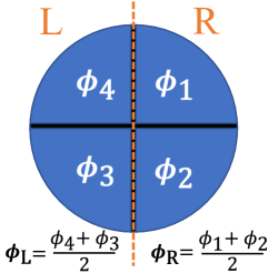
Figure 6: The phase terms at each photodiode quadrant of a circular QPD are labeled in the diagram, bisected for left “L” and right “R” as in the DWS description.

Now, consider that in Eq. 16 the geometric TTL phase clearly has no quadrant dependence, so this geometric TTL phase is canceled in the DWS formulation. More importantly, however, geometric TTL contributes equally to both LPS formulations. This motivates us to work with a nominal setup that has zero TTL coupling and simulate then cases of primarily non-geometric TTL introduced by our misalignment parameters. Thereby, we focus on scenarios where the non-geometric TTL is predominant, leading to differences between LPSA and LPSC. This is true except for one case, where we show that geometric TTL dominates and LPSA and LPSC perform equally, as expected.

The definitions we have provided for the LPS and DWS signal in this section represent those of the conventional signal extraction architecture [9, 10], where each of the four quadrants of the QPD are tracked separately. The architecture currently proposed for LISA, described in [23], would instead employ a different set of four tracking loops operating directly on the length and angles. Each loop can be individually optimized for the dynamic range and noise characteristics of that particular observable. This allows for an improvement in signal-to-noise ratio and robustness to cycle slips, and it is especially useful at the ISI where low received beam powers are expected. It was likewise shown in [23] that for sufficiently high loop gains, the new architecture is equivalent to the LPSA. Therefore we consider here that the conventional definition remains appropriate for simulation of the TMI, and we thus also compare the performance of the phase signal of the new architecture under the assumption of a high-loop gain (LPSA) with the performance of one alternative signal definition (LPSC). In the next section, we report the results of our study in terms of these signals.

4 Simulation results

In this section, we present simulation results for the two LPS candidates: LPSC and LPSA.

4.1 Results for variations in the waist sizes of the beams

[] []

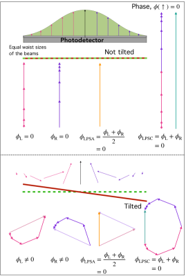
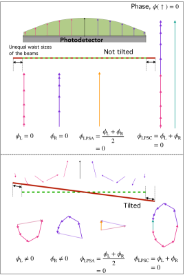
Figure 7: Graphical illustration of vanishing non-geometric TTL coupling in two cases with beam rotation around the centre of a QPD. Image (a) shows the case of matched waist sizes, image (b) a case where the MB (red flat wavefront), has a larger waist than the LO (green-dashed flat wavefront). The total LPSA ($1/k$ times the angle of the orange vector) and LPSC ($1/k$ times the angle of the green vector) signals are estimated via vector sums of the individual phasors. See text and [8] for more information.

We conducted simulations which varied waist sizes of the MB and LO separately. Here, we varied the waist radii by $\pm 10\,\%$ in steps of $5\,\%$ around the nominal value of $0.402\text{\,}\mathrm{m}\mathrm{m}$. This resulted in a negligible TTL coupling, due only to numerical error ($\mathcal{O}$ $\sim${10}^{-17}\text{\,}\mathrm{m}$$ to ${10}^{-23}\text{\,}\mathrm{m}$) for all simulation methods and geometries. In this scenario, geometric TTL coupling plays no role due to the absence of differences in the optical pathlengths of the beams. Since the total TTL coupling is negligible, we can deduce that the non-geometric TTL is likewise negligible in this specific case. We explain this graphically in Fig. 7.

In the two scenarios of Fig. 7, the LO and MB are Gaussian beams of equal waist sizes, while in Fig. 7 the waist sizes are unequal. In the top of each figure, we sketch a rough estimate of the amplitude resulting from the superposition of the two beams at the photodetector. This amplitude shows slight variation as the MB waist size varies and serves for defining the lengths of the vectors (phasors) in the lower parts of the images. Below these amplitude diagrams in each subfigure, we trace the wavefronts of the two beams in red (MB) and green (LO) and allow for clipping when the MB size is varied in Fig. 7. Each of these wavefronts is flat, due to the waists being located on the photodiode (cf. Sections 2.3 and 2). The amount by which the red wavefront is above or below the green wavefront defines the angle of the corresponding phasors. The bottom half of each subfigure depicts these same wavefronts respectively for the cases in which the MB is tilted with respect to the LO.

For all four scenarios, we explicitly show the sum of the phasors reduces to zero, signifying that the non-geometric TTL is negligible for the case of waist size variation due to this phase antisymmetry. Please note that the $\phi_{\text{LPSA}}$ was illustrated via a vector sum. This is not the usual procedure, but possible in this specific case due to the equal lengths of the phasors illustrating the complex amplitudes on the left (light red phasor) and right (light purple phasor) halves of the photodiode. This implies that for such cases with equal amplitude on the left and right halves, the LPSA and LPSC are identical. Please see [8] for a detailed explanation of this type of illustration.

4.2 Results for lateral offset of beam axes

In this simulation, we tested the TTL coupling due to a lateral offset ($x_{\textrm{off}}$) of the MB with respect to the QPD center. This is shown in Fig. 8 and includes an optical pathlength difference $L_{\mathrm{OPD}}$ (as a blue segment of the MB), which for this scenario is

$$L_{\mathrm{OPD}}(\alpha,x_{\textrm{off,MB}})=-x_{\textrm{off,MB}}\tan(\alpha)\approx-x_{\textrm{off,MB}}\alpha\,.$$ (20)

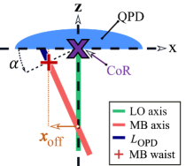
Figure 8: Test geometry where the measurement beam’s (MB) center of rotation remains the QPD center (shown by a purple “X”), but the beam axis is laterally offset by a distance $x_{\textrm{off}}$ before rotating in $\alpha$. These rotations yield an additional pathlength $L_{\textrm{OPD}}$ extending from the red “+” which marks the new MB waist to the intersection point of the beam axis with the photodiode. The depiction is not to scale, as even the largest offset of 0.2 mm still allows beam overlap.

The optical pathlength difference $L_{\mathrm{OPD}}$ defined in Eq. 20 was derived from the difference between the propagation distance of the tilted MB and the propagated distance of the nominal MB. However, this equals the definition given in LABEL:{eq:TTL_breakdown}. To see this, one can set $k_{\textrm{MB}}=k_{\textrm{LO}}$ and neglect the non-geometric elements in this equation, to find

$$L_{\textrm{OPD}}(\alpha)\Rightarrow\left[D_{\mathrm{MB}}(\alpha)-D_{\mathrm{LO}}(\alpha)\right]-\left[D_{\mathrm{MB}}(0)-D_{\mathrm{LO}}(0)\right]\;.$$ (21)

The propagation distances for the LO cancel from this equation, because the LO does not rotate. This results in the described comparison of the MB propagation distances.

We also quantify non-geometric contributions in each test via a functional fitting of the LPS to its misalignment. Calling each misalignment parameter $\chi$, the $L_{\mathrm{OPD}}$ and non-geometric contributions combine to induce a change to the LPS, $\Delta\mathrm{LPS}$, for which we provide a functional fitting of the form

$$\Delta\textrm{LPS}(\alpha,\chi)\approx L_{\mathrm{OPD}}+\sum_{i,j=1}^{4}\left(c_{i,j}\alpha^{i}\chi^{j}\right)\;.$$ (22)

Here, $c_{i,j}$ is the scaling coefficient for a tilt, $\alpha$, of order $i$ coupled to a particular misalignment, $\chi$, of order $j$. These we accurately truncate to fourth order (i.e., a cutoff of $i,j=4$). The $c_{i,j}$ non-zero values therefore represent the strongest coupling coefficients in a polynomial expansion of non-geometric TTL obtained via least squares-fit in terms of beam tilt, $\alpha$. Square QPD coefficients in this fitting were derived from data of the Analytical Method, while those for the circular QPD were from IfoCAD data. These two methods are sufficient to generate third-order coefficients. For instance, the functional form for this MB tilt-misalignment coupling (where $\chi=x_{\textrm{off,MB}}$) is

$$\Delta\textrm{LPS}(\alpha,x_{\textrm{off,MB}})\approx L_{\mathrm{OPD}}+\alpha(c_{1,1}x_{\textrm{off,MB}}+c_{1,3}x_{\textrm{off,MB}}^{3})\;.$$ (23)

Values calculated from fitting to this coupling are shown in Table 2.

Table 2: Fit coefficients for lateral offsets of the MB’s beam axis ($x_{\textrm{off,MB}}$).

Coefficient	Small Square QPD Range	Circular QPD Range	Large Square QPD Range
LPSC $c_{1,1}$ $\left(\frac{\mathrm{pm}}{(\mathrm{mm})(\upmu\mathrm{rad})}\right)$	$(6.450\pm 0.017)\times 10^{2}$	$(5.544\pm 0.013)\times 10^{2}$	$(5.247\pm 0.016)\times 10^{2}$
LPSA $c_{1,1}$ $\left(\frac{\mathrm{pm}}{(\mathrm{mm})(\upmu\mathrm{rad})}\right)$	$(8.996\pm 0.002)\times 10^{2}$	$(8.604\pm 0.001)\times 10^{2}$	$(8.488)\times 10^{2}$
LPSC $c_{1,3}$ $\left(\frac{\mathrm{pm}}{(\mathrm{mm}^{3})(\upmu\mathrm{rad})}\right)$	$(2.150\pm 0.046)\times 10^{2}$	$(2.108\pm 0.034)\times 10^{2}$	$(2.211\pm 0.036)\times 10^{2}$
LPSA $c_{1,3}$ $\left(\frac{\mathrm{pm}}{(\mathrm{mm}^{3})(\upmu\mathrm{rad})}\right)$	$(1.637\pm 0.008)\times 10^{1}$	$(6.651\pm 0.284)$	$(5.850\pm 0.500)$

Plots of LPSC and LPSA calculated by the three simulation methods are shown in Fig. 9 for the “small” $\sqrt{2}/2$ mm-width and “large” 1 mm-width square QPDs, respectively, against the IfoCAD Method 1 mm-diameter circular QPD. These show that the LPSA is less susceptible to TTL coupling due to lateral offsets of the MB’s axis, as the LPSC magnitude is nearly three times greater. These results also demonstrate the influence of QPD geometry on pathlength noise, particularly, the discrepancy between the circular and square QPD geometries. While the plots emphasize differences for interferometric simulation with the two square QPD sizes, they also display reasonable agreement ($\pm 100\,\upmu$rad) for the 1 mm circular and large square QPDs (which more closely mimic the circular QPD). The square QPD implementation in IfoCAD was verified to agree well with the other two methods (cf. A).

[]

[]

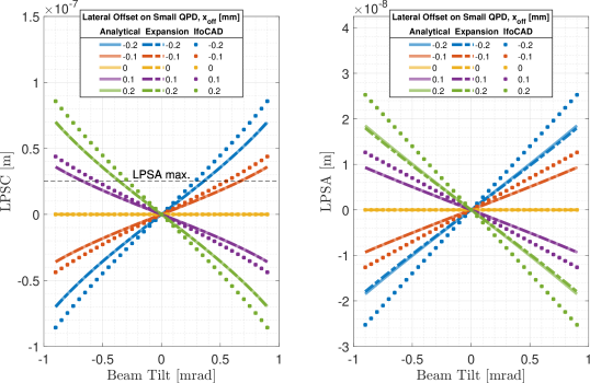
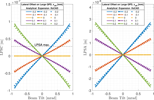
Figure 9: TTL coupling in the case of lateral shifts of the measurement beam. Shown are the LPSC (left figures) and LPSA (right figures) computed with the analytic and expansion method for “small” square QPDs (upper figures, diameter $1/\sqrt{2}\,$mm) and “large” square QPDs (lower figures, $1\,$mm diameter) in comparison to the results for $1\,$mm circular QPDs implemented in IfoCAD. The dashed line, “LPSA max.”, denotes the maximal LPSA value in each row of plots for comparison of magnitudes in the two formulations.

Now, consider the effect of offsets to the LO, rather than the MB, while still applying a rotation to the MB axis. When we laterally offset the LO instead of the MB by $x_{\textrm{off}}$, the new scenario is as depicted in Fig. 10.

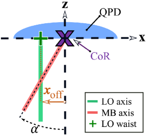
Figure 10: Test geometry where measurement beam center of rotation remains the QPD center (shown by a purple “X”), but the LO waist is laterally offset a distance $x_{\textrm{off}}$. The green “+” marks the new LO waist location at the photodiode.

For this lateral offset of the LO instead of the MB, the pathlength signals look nearly identical to the plots of Fig. 9. We have verified this equality to four significant digits beyond the LPS ranges shown in Fig. 9. Although the total couplings agree at this precision, the first-order coefficients in Table 3 for non-geometric TTL fittings differ from the MB lateral offset case in Table 2. In changing from an MB offset to an LO offset, the geometric TTL goes to zero so that the functional form for the total TTL coupling in this case is

$$\Delta\textrm{LPS}(\alpha,x_{\textrm{off,LO}})\approx\alpha(c_{1,1}x_{\textrm{off,LO}}+c_{1,3}x_{\textrm{off,LO}}^{3})\;.$$ (24)

However, since this total TTL coupling is the same as for the shifted MB-axis, the missing geometric TTL-term here must be nearly compensated by an additional non-geometric TTL contribution. Small differences between the two setups of Figs. 8 and 10 are expected due to asymmetrical clipping across the QPD inactive regions.

Table 3: Fit coefficients for lateral offset of the LO ($x_{\textrm{off,LO}}$).

Coefficient	Small Square QPD Range	Circular QPD Range	Large Square QPD Range
LPSC $c_{1,1}$ $\left(\frac{\mathrm{pm}}{(\mathrm{mm})(\upmu\mathrm{rad})}\right)$	$(-3.550\pm 0.017)\times 10^{2}$	$(-4.457\pm 0.013)\times 10^{2}$	$(-4.754\pm 0.017)\times 10^{2}$
LPSA $c_{1,1}$ $\left(\frac{\mathrm{pm}}{(\mathrm{mm})(\upmu\mathrm{rad})}\right)$	$(-1.004\pm 0.002)\times 10^{2}$	$(-1.397\pm 0.001)\times 10^{2}$	$(-1.512\pm 0.001)\times 10^{2}$
LPSC $c_{1,3}$ $\left(\frac{\mathrm{pm}}{(\mathrm{mm}^{3})(\upmu\mathrm{rad})}\right)$	$(2.150\pm 0.046)\times 10^{2}$	$(2.108\pm 0.034)\times 10^{2}$	$(2.211\pm 0.036)\times 10^{2}$
LPSA $c_{1,3}$ $\left(\frac{\mathrm{pm}}{(\mathrm{mm}^{3})(\upmu\mathrm{rad})}\right)$	$(1.637\pm 0.008)\times 10^{1}$	$(6.651\pm 0.284)$	$(5.850\pm 0.500)$

Please note that it might appear from the coupling coefficients that the TTL effect in the LPSC formulation is below that of the LPSA formulation. However, the cancellation between geometric and non-geometric TTL results here in lower TTL noise for LPSA than LPSC.

4.3 Results for lateral offset of measurement beam center of rotation

In this test, we laterally shifted the MB’s center of rotation ($x_{\textrm{cor}}$), as illustrated in Fig. 11. The optical pathlength difference between the MB in the tilted and non-tilted case is

$$L_{\mathrm{OPD}}(\alpha,x_{\textrm{cor}})=x_{\textrm{cor}}\tan(\alpha)\approx x_{\textrm{cor}}\alpha\,.$$ (25)

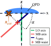
Figure 11: Test geometry where the measurement beam center of rotation is laterally offset along the $x$-axis to $x_{\textrm{cor}}$, which is represented as an orange “$\times$”. The longitudinal center of rotation is still ${z=0}$. These rotations yield additional pathlength $L_{\textrm{OPD}}$ extending from the new MB waist location (the red “+”). Here, the rotation and offset are negative values.

Notably, this case yields identical results for LPSA and LPSC, as shown in Fig. 12.

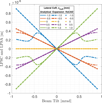
Figure 12: The plots equivalently show LPSC and LPSA for a variation to the measurement beam lateral center of rotation ($x_{\textrm{cor}}$) for values of $\pm\{0,\,0.5,\,1\}\,$mm. Only LPSC values were plotted because differences between the two datasets for all methods were due to numerical error (on the order of $10^{-10}\,$m). The Expansion method shows divergence from the other two methods for large tilt, as expected, due to limitations of the approximation for large static misalignments.

The similarity in the two signals is because the TTL coupling is dominated by the geometric contribution of the relatively large $x_{\textrm{cor}}$ variation itself. Geometrically equivalent to a lateral offset of the MB, this generates the same type of lever arm as in $x_{\textrm{off}}$ case, thus producing an equivalent (up to sign) geometric TTL. The functional fitting here was performed again using the Analytical method for the square quadrant photodiodes (QPDs) and IfoCAD for the circular, and takes the form:

$$\Delta\textrm{LPS}(\alpha,x_{\textrm{cor}})\approx L_{\mathrm{OPD}}+x_{\textrm{cor}}(c_{1,1}\alpha+c_{3,1}\alpha^{3})\,.$$ (26)

The fit coefficients we obtained are listed in Table 4.

Table 4: Fit coefficients for lateral offset in the MB center of rotation ($x_{\textrm{cor,MB}}$).

Coefficient	Small Square QPD Range	Circular QPD Range	Large Square QPD Range
LPSC $c_{1,1}$ $\left(\frac{\mathrm{pm}}{(\mathrm{mm})(\upmu\mathrm{rad})}\right)$	$(2.317\pm 0.021)\times 10^{-4}$	$(1.991\pm 0.012)\times 10^{-4}$	$(1.880\pm 0.011)\times 10^{-4}$
LPSA $c_{1,1}$ $\left(\frac{\mathrm{pm}}{(\mathrm{mm})(\upmu\mathrm{rad})}\right)$	$(2.299\pm 0.003)\times 10^{-4}$	$(1.977\pm 0.001)\times 10^{-4}$	$(1.869\pm 0.003)\times 10^{-4}$
LPSC $c_{3,1}$ $\left(\frac{\mathrm{pm}}{(\mathrm{mm})(\upmu\mathrm{rad}^{3})}\right)$	$(3.492\pm 0.098)\times 10^{-10}$	$(3.374\pm 0.065)\times 10^{-10}$	$(3.430\pm 0.050)\times 10^{-10}$
LPSA $c_{3,1}$ $\left(\frac{\mathrm{pm}}{(\mathrm{mm})(\upmu\mathrm{rad}^{3})}\right)$	$(4.560\pm 0.006)\times 10^{-10}$	$(4.481\pm 0.005)\times 10^{-10}$	$(4.488\pm 0.009)\times 10^{-10}$

The relatively large offsets used in this scenario are of particular detriment to the Expansion method - the offset to the CoR of $1\,$mm, for instance, is roughly twice the beam size and induces a pathlength difference $L_{\mathrm{OPD}}\simeq 0.3\,\upmu$m at $300\,\upmu$rad. Regardless, it is clear that the geometric TTL dominates in this case. This is prominently visible when comparing the linear geometric contribution, defined in Eq. 25, with the linear non-geometric contribution, $x_{\textrm{cor}}(c_{1,1}\alpha)$ from Eq. 26. Here, the non-geometric coefficient $c_{1,1}$, with values of approximately $2\times 10^{-4}$ pm/mm/$\upmu$rad = $2\times 10^{-7}$ $\mathrm{rad}^{-1}$ as listed in Table 4, needs to be compared with a factor $c_{1,1}^{\text{geom}}$ (which we did not explicitly define in Eq. 25) of value $c_{1,1}^{\text{geom}}=$1 rad^-1. Thereby, the geometric TTL is dominating in this case by nearly 7 orders of magnitude.

4.4 Results for longitudinal offset of beam waists

In this test, we longitudinally shifted the position of the MB waist by $z_{\textrm{off}}$ along its beam axis, as illustrated in Fig. 13. Here, the additional pathlength from misalignment is a tilt-independent offset which produces a constant phase shift, hence

$$L_{\mathrm{OPD}}(\alpha,z_{\textrm{off}})=0\,.$$ (27)

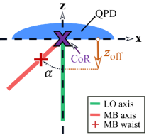
Figure 13: Test geometry where the measurement beam’s center of rotation remains the QPD center (purple “$\times$”), but the waist (red “+”) is longitudinally offset by a distance $z_{\textrm{off}}$ before rotation in $\alpha$. Note that $L_{OPD}$ is independent of angle and thus zero for this coupling. In this depiction, the rotation and offset are negative values.

Results for the LPSC and LPSA signals are shown in Fig. 14. Clearly, LPSA is subject to roughly four times less TTL noise than LPSC for the case of longitudinal waist position offsets. Disparity between IfoCAD and the two other methods is again due only to difference in QPD geometry, which we verified with square QPD implementation in IfoCAD (cf. A).

Figure 14: The plots show LPSC (left) and LPSA (right) for large $1\,$mm square QPD (“Analytical”, “Expansion”) or a circular QPD (“IfoCAD”) following longitudinal offset of the MB waist and tilt of its beam axis about the QPD center. In this case, LPSA again shows significantly smaller noise coupling than LPSC. This is made more evident by the dashed “LPSA max” line which denotes the maximal value from the LPSA plots.

Because $L_{\mathrm{OPD}}$ goes to zero here, the total TTL contributions from this misalignment coupling can be written as

$$\Delta\textrm{LPS}(\alpha,z_{\textrm{off}})\approx\alpha^{2}\left(c_{2,1}z_{\mathrm{off}}+c_{2,3}z_{\mathrm{off}}^{3}\right).$$ (28)

We present coupling coefficients for this case in Table 5.

Table 5: Coefficients for TTL effects from MB longitudinal offsets ($z_{\textrm{off,MB}}$).

Coefficient	Small Square QPD Range	Circular QPD Range	Large Square QPD Range
LPSC $c_{2,1}$ $\left(\frac{\mathrm{pm}}{(\mathrm{mm})(\upmu\mathrm{rad}^{2})}\right)$	$(-3.575\pm 0.018)\times 10^{-5}$	$-6.608\times 10^{-5}$	$(-8.503\pm 0.011)\times 10^{-5}$
LPSA $c_{2,1}$ $\left(\frac{\mathrm{pm}}{(\mathrm{mm})(\upmu\mathrm{rad})^{2}}\right)$	$(-6.750\pm 0.038)\times 10^{-6}$	$(-1.745\pm 0.004)\times 10^{-5}$	$(-2.348\pm 0.018)\times 10^{-5}$
LPSC $c_{2,3}$ $\left(\frac{\mathrm{pm}}{(\mathrm{mm}^{3})(\upmu\mathrm{rad}^{2})}\right)$	$(1.198\pm 0.005)\times 10^{-10}$	$1.872\times 10^{-10}$	$(1.888\pm 0.005)\times 10^{-10}$
LPSA $c_{2,3}$ $\left(\frac{\mathrm{pm}}{(\mathrm{mm}^{3})(\upmu\mathrm{rad}^{2})}\right)$	$(2.995\pm 0.020)\times 10^{-11}$	$(6.190\pm 0.001)\times 10^{-11}$	$(6.779\pm 0.025)\times 10^{-11}$

Conversely, if we instead offset the LO beam (while still rotating the MB) the resulting coefficients are those in Table 6.

Table 6: Coefficients for TTL effects from LO longitudinal offsets ($z_{\textrm{off,LO}}$).

Coefficient	Small Square QPD Range	Circular QPD Range	Large Square QPD Range
LPSC $c_{2,1}$ $\left(\frac{\mathrm{pm}}{(\mathrm{mm})(\upmu\mathrm{rad}^{2})}\right)$	$(3.575\pm 0.018)\times 10^{-5}$	$6.608\times 10^{-5}$	$(8.503\pm 0.011)\times 10^{-5}$
LPSA $c_{2,1}$ $\left(\frac{\mathrm{pm}}{(\mathrm{mm})(\upmu\mathrm{rad})^{2}}\right)$	$(6.750\pm 0.038)\times 10^{-6}$	$(1.745\pm 0.004)\times 10^{-5}$	$(2.348\pm 0.018)\times 10^{-5}$
LPSC $c_{2,3}$ $\left(\frac{\mathrm{pm}}{(\mathrm{mm}^{3})(\upmu\mathrm{rad}^{2})}\right)$	$(-1.198\pm 0.005)\times 10^{-10}$	$-1.872\times 10^{-10}$	$(-1.888\pm 0.005)\times 10^{-10}$
LPSA $c_{2,3}$ $\left(\frac{\mathrm{pm}}{(\mathrm{mm}^{3})(\upmu\mathrm{rad}^{2})}\right)$	$(-2.995\pm 0.020)\times 10^{-11}$	$(-6.190\pm 0.001)\times 10^{-11}$	$(-6.779\pm 0.025)\times 10^{-11}$

It is obvious the coefficients differ between Table 5 and Table 6 only in sign. The plots for the case of shifting the LO instead are identical to those of Fig. 14 except for a sign inversion, but they are not shown here for the sake of brevity. This indicates that TTL noise contributions here depend only on the initial relative longitudinal offset between beam waists. Therefore, a more succinct form of Eq. 28 for LPS contribution in the case of longitudinal offsets is

$$\Delta\textrm{LPS}(\alpha,z_{\textrm{off}})\approx\alpha^{2}\left(c_{2,1}\Delta z+c_{2,3}\Delta z^{3}\right)\,$$ (29)

where $\Delta z=z_{\textrm{off,MB}}-z_{\textrm{off,LO}}$ is the distance between beam waists.

4.5 Results for longitudinal offset of measurement beam center of rotation

In this final test, we varied the MB’s longitudinal center of rotation ($z_{\textrm{cor}}$) point along the optical axis, as illustrated by Fig. 15. The geometric TTL contribution here is

$$L_{\mathrm{OPD}}=z_{\textrm{cor}}\left(1-\frac{1}{\cos\alpha}\right)\,.$$ (30)

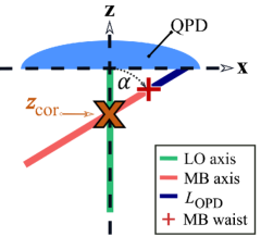
Figure 15: Test geometry where the measurement beam center of rotation is shifted longitudinally along the $z$-axis by $z_{\textrm{cor}}$. The orange “$\times$” represents the new rotation point. These rotations yield additional pathlength $L_{\textrm{OPD}}$ extending from the new MB waist location (the red “+”). Here, the rotation and offset are both negative values.

The LPS results for this test are shown in Fig. 16. Here, we observe a significant difference between the LPSC calculated with IfoCAD’s circular QPD when compared against the other two methods’ large square QPD results. This disparity is especially apparent beyond $\pm 100\,$$\upmu$rad in the LPSC. We verified via square QPD implementation in IfoCAD that this disparity is solely due to QPD geometry (cf. A).

Figure 16: This figure shows plots of LPSC and LPSA for variation to the MB longitudinal center of rotation ($z_{\textrm{cor}}$) of $\pm\{0,\,2.5,\,5\}$ mm for the large square photodiode (“Analytical”,“Expansion”) and circular photodiode (“IfoCAD”). This is the single case where LPSC shows smaller noise coupling than LPSA, which is emphasized by the dashed “LPSC max” line denoting the maximal value from the LPSC plots.

The total TTL effects can be described accurately via

$$\Delta\textrm{LPS}(\alpha,z_{\textrm{cor}})\approx L_{\mathrm{OPD}}+z_{\mathrm{cor}}\left(c_{2,1}\alpha^{2}+c_{4,1}\alpha^{4}\right)\;.$$ (31)

These coefficients are shown in Table 7. The second-order OPD effect couples to interferometric phase readout and approaches $2\,$nm at $1\,$mrad of beam tilt for $z_{\textrm{cor}}=5\,$mm. Ideally, imaging systems in the beam path would mitigate geometric coupling so that the pivot of the beam is re-oriented onto the QPD center.

Displacing the CoR along the beam axis is a case of vanishing TTL when computed on a large single-element photodiode (SEPD) (cf. [11]). Using the complex-sum formalism to compute the coupling for the signal on a finite-sized QPD is almost equivalent to calculating the total phase across the PD surface as a single element, except for some signal power loss at the QPD’s slit and edges. The LPSA formalism does not mimic the signal generation on a large SEPD in the same quality as the LPSC formalism does. Hence, in this specific case, we expect the coupling in the LPSC to be less than in the LPSA, and this is what can be seen in Fig. 16. Therefore, this case is the first and only one of our 5 cases where the LPSC is less susceptible to TTL coupling than the LPSA formalism.

Table 7: Coefficients for longitudinal offset in MB center of rotation ($z_{\textrm{cor,MB}}$).

Coefficient	Small Square QPD Range	Circular QPD Range	Large Square QPD Range
LPSC $c_{2,1}$ $\left(\frac{\mathrm{pm}}{(\mathrm{mm})(\upmu\mathrm{rad})^{2}}\right)$	$(-6.484\pm 0.020)\times 10^{-4}$	$(-5.576\pm 0.016)\times 10^{-4}$	$(-5.278\pm 0.015)\times 10^{-4}$
LPSA $c_{2,1}$ $\left(\frac{\mathrm{pm}}{(\mathrm{mm})(\upmu\mathrm{rad}^{2})}\right)$	$(-8.997\pm 0.001)\times 10^{-4}$	$(-8.603\pm 0.001)\times 10^{-4}$	$(-8.487\pm 0.003)\times 10^{-4}$
LPSC $c_{4,1}$ $\left(\frac{\mathrm{pm}}{(\mathrm{mm})(\upmu\mathrm{rad}^{4})}\right)$	$(5.754\pm 0.746)\times 10^{-11}$	$(5.492\pm 0.613)\times 10^{-11}$	$(5.712\pm 0.595)\times 10^{-11}$
LPSA $c_{4,1}$ $\left(\frac{\mathrm{pm}}{(\mathrm{mm})(\upmu\mathrm{rad}^{4})}\right)$	$(3.781\pm 0.052)\times 10^{-12}$	$(7.490\pm 6.710)\times 10^{-13}$	$(4.930\pm 7.620)\times 10^{-13}$

4.6 Removing linear tilt-to-length coupling by applying a model fit

In Sections 4.2, 4.3, 4.5 and 4.4, we have shown four instances of TTL coupling caused by misalignment in the initially defined setup. Some of our resulting plots of the longitudinal pathlength signals show notably non-linear TTL coupling across the examined beam angle range (i.e., $\pm$900\text{\,}\upmu\mathrm{r}\mathrm{a}\mathrm{d}$$). In practice, the SC’s angular jitter will be at the $\text{\,}\mathrm{n}\mathrm{r}\mathrm{a}\mathrm{d}\mathrm{/}\sqrt{Hz}$ level, accompanied by a µrad-level angular offset (referred to as a DC offset). Thereby, the jitter will probe the nonlinear curve in a very small range around some point. Consequently, the TTL coupling expected in LISA will resemble a dominantly first order Taylor expansion of the presented curves, and it will be centered around the DC offset angle. Hence, one possible mitigation scheme involves fitting the TTL coupling with a linear model and removing this component from the data in the post-processing, as discussed in the works of [24, 25].

In this subsection, we investigate the non-linear TTL residuals of our simulated pathlength signals after this linear subtraction scheme. In [25], for instance, an approximately white jitter of $5\,$$\text{\,}\mathrm{n}\mathrm{r}\mathrm{a}\mathrm{d}\mathrm{/}\sqrt{Hz}$ is projected for LISA in roughly the $3\text{\,}\mathrm{m}\mathrm{H}\mathrm{z}100\text{\,}\mathrm{m}\mathrm{H}\mathrm{z}$ band. We use this $5\,$nrad jitter value for testing the relevance of the non-linear TTL coupling of the TMI. Here, the beam tilt seen at the QPD level is scaled by a factor of five (2 for the TM round-trip, and 2.5 for the magnification factor (cf. Section 2.3)). Thus, we expect the MB tilt of our test cases to probe around a $\pm 25\,$nrad region, centered at some DC offset. We assume such offsets on the order of 10s of $\text{\,}\upmu\mathrm{r}\mathrm{a}\mathrm{d}$ to be realistic for the LISA test mass interferometers (TMIs).

Under these considerations, our implementation of a linear TTL subtraction follows these steps:

• We first apply a fourth order polynomial fit to our results of both LPSA and LPSC for each misalignment test case.

• We then linearize these fits in $\pm 25\,$nrad beam jitter regions, which are each centered at $50\,\upmu$rad steps of our $\pm 900\,$$\text{\,}\upmu\mathrm{r}\mathrm{a}\mathrm{d}$ beam tilt range. This allows us to probe the signals around various DC offset angles in approximately linear regimes.

• Finally, we compute length residuals when the linear fit is subtracted off the fourth-order fit function.

The plots in Fig. 17 and Fig. 18 show the corresponding residuals in both signals (LPSC and LPSA, respectively) for the largest test value in each type of misalignment. These data are computed from the IfoCAD circular QPD results. In the figures, each row shows plots for one particular misalignment. The first column shows the fourth order fit and its good overlap with the original data. The second column shows the residuals at each of the $\pm 25\,$nrad linear fit regions. Due to the very small x-range we used for each colored line, the residuals appear as vertical lines, but they are polynomial functions (except for numerical noise). This is made apparent in the third column, which shows “zoomed-in” plots of each fit, at the $\sim$nrad scale.

Figure 17: Plots of LPSC fits and residuals for each misalignment case (from IfoCAD circular QPD data) as explained in the text.

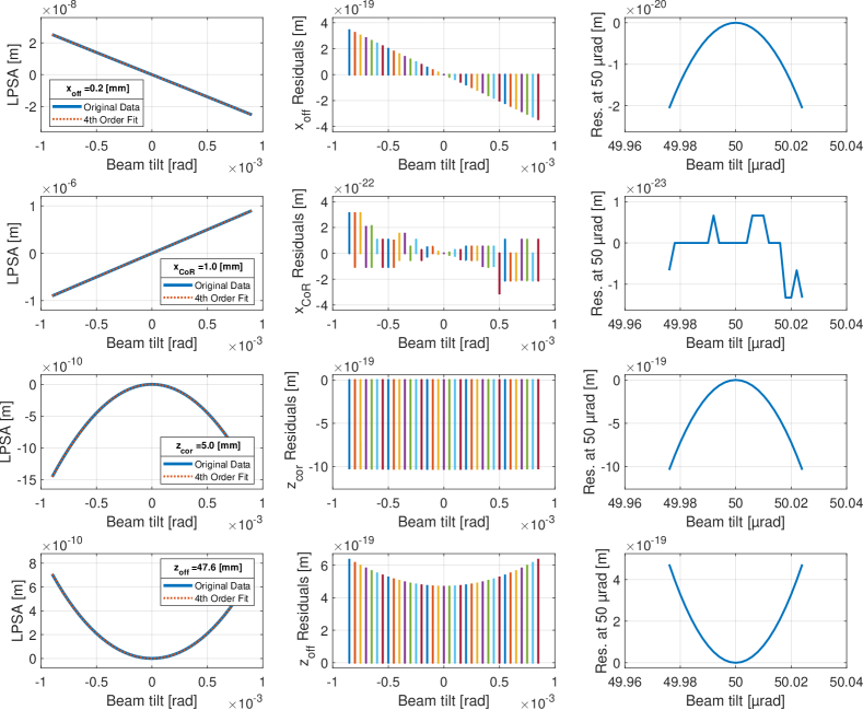
Figure 18: Plots of LPSA fits and residuals for each misalignment case (from IfoCAD circular QPD data) as explained in the text.

These plots show very optimistically that the residuals following this subtraction scheme are $\mathcal{O}$($10^{-22}$ to $10^{-17}\,$m), far below the picometer-level criteria required for LISA. Hence, the non-linear contributions to TTL noise for all of the cases we have tested in this work are negligible under the assumptions of our subtraction scheme.

5 Summary and conclusion

We have shown case-by-case simulations of the tilt-to-length coupling for the LISA TMI in two types of signal formulations: the averaged phase (LPSA) and the complex sum (LPSC). For all cases, we have tested three different methods, and have found good agreement of the results, particularly if identical photodiode geometries were used.

In total, we have tested five different cases of static misalignments. In the first case, we tested waist size mismatches (Section 4.1), which led to vanishing TTL in both signal types. We also tested two cases of misalignment in which LPSA showed less TTL coupling than LPSC. These were the case of lateral offset of the MB (or LO) beam axis (Section 4.2) and the case of longitudinal offset of the MB waist location (Section 4.4). A fourth case, lateral offset of the MB center of rotation (Section 4.3), proved to be dominated by geometric TTL coupling so that the two formulations performed equally.

In the fifth case, we investigated variation to the MB longitudinal center of rotation (Section 4.5). This is an exceptional case, where a large SEPD would not sense any TTL coupling. The LPSC method is the best approximation of the longitudinal pathlength signal of an SEPD obtainable from a QPD. Therefore, the LPSC shows the best approximation of the SEPD’s zero-coupling, and, therefore, less TTL coupling than the LPSA signal.

For LISA it is currently expected that the TTL coupling will be reduced by subtracting a linear fit model from the measured LPS data. The magnitude of the TTL coupling coefficients prior to subtraction influences the residual noise level obtained after this subtraction is performed. Therefore, the choice of the LPS formalism might indeed have an impact on the final noise performance. From the results we have presented here, it appears that the LPSA formulation is the favorable choice for the TMI. However, the TMI is known to be subject to significantly less TTL noise than the ISI. Therefore, an extension of this study to the ISI is needed to finally judge which signal formalism is a better choice there for TTL suppression.

Finally, we investigated the non-linear TTL contributions in the TMI. For this, we subtracted a linear fit model from our LPS-data and tested the magnitude of the coupling for jitter levels currently expected for LISA. We found the non-linear TTL contributions to be negligible in all of our test cases of misalignments in the TMI relative to LISA requirements.

6 Acknowledgments

We thank Josep Sanjuan for providing his valuable insight and the LISA Consortium’s TTL Expert Group as well as Gerhard Heinzel for inspiring discussions.
This work was supported by NASA grant 80NSSC19K0324 for contributions of the team in Florida, US. The Albert Einstein Institute acknowledges support of the German Space Agency, DLR and by the Federal Ministry for Economic Affairs and Climate Action based on a resolution of the German Bundestag (FKZ 50OQ0501, FKZ 50OQ1601 and FKZ 50OQ1801). Additionally, Gudrun Wanner acknowledges funding by Deutsche Forschungsgemeinschaft (DFG) via its Cluster of Excellence QuantumFrontiers (EXC 2123, Project ID 390837967). Furthermore, Gudrun Wanner and Megha Dave acknowledge support by the DFG Cluster of Excellence PhoenixD (EXC 2122, Project ID 390833453) and thank both clusters for the opportunities and excellent scientific exchange via the Topical Group “Optical Simulations” and the Research Area “S” on Simulations.
This work has also been supported by the Max Planck Society and the Chinese Academy of Sciences (CAS) in the framework of the LEGACY cooperation on low-frequency gravitational wave astronomy (M.IF.A.QOP18098, CAS’s Strategic Pioneer Program on Space Science XDA1502110201). The National Key R&D Program of China (2020YFC2200100) provided the funding that supported the contributions made by Mengyuan Zhao in this work.

Appendix A Verification of the IfoCAD square photodiode geometry

Plots of longitudinal pathlength signals of Section 4 only showed the IfoCAD method results for the circular QPD geometry. However, disparities existed between these results and the two other methods which were particularly significant for certain misalignments. These were the $x_{\textrm{off}}$ (Section 4.2), $z_{\textrm{off}}$ (Section 4.4), and $z_{\textrm{cor}}$ (Section 4.5) cases, which we now present here as verification that all three methods very closely agree when the same geometry is applied. All of these plots show LPSC and LPSA results for only the $1\,$mm width square QPD.

Figure 19: Variation to the measurement beam lateral center of rotation ($x_{\textrm{off}}$), where all three methods use a $1\,$mm width square QPD (cf. Fig. 9).

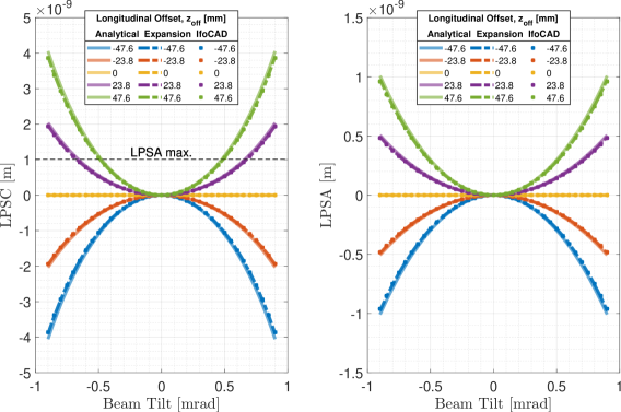
Figure 20: Variation to the measurement beam waist offset ($z_{\textrm{off}}$), where all three methods use a $1\,$mm width square QPD (cf. Fig. 14).

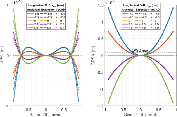
Figure 21: Variation to the measurement beam longitudinal center of rotation ($z_{\textrm{cor}}$), where all three methods use a $1\,$mm width square QPD (cf. Fig. 16).

References

References

- [1] European Space Agency 2024 Capturing the ripples of spacetime: LISA gets go-ahead accessed: 1st February 2024 URL https://www.esa.int/Science_Exploration/Space_Science/Capturing_the_ripples_of_spacetime_LISA_gets_go-ahead
- [2] Amaro-Seoane P et al. 2017 Laser interferometer space antenna URL https://arxiv.org/abs/1702.00786
- [3] Armano M et al. 2018 Phys. Rev. Lett. 120(6) 061101 URL https://link.aps.org/doi/10.1103/PhysRevLett.120.061101
- [4] Armano M, Audley H, Baird J, Binetruy P, Born M, Bortoluzzi D, Castelli E, Cavalleri A, Cesarini A, Cruise A M, Danzmann K, de Deus Silva M, Diepholz I, Dixon G, Dolesi R, Ferraioli L, Ferroni V, Fitzsimons E D, Freschi M, Gesa L, Giardini D, Gibert F, Giusteri R, Grimani C, Grzymisch J, Harrison I, Hartig M S, Heinzel G, Hewitson M, Hollington D, Hoyland D, Hueller M, Inchauspé H, Jennrich O, Jetzer P, Johann U, Johlander B, Karnesis N, Kaune B, Killow C J, Korsakova N, Lobo J A, López-Zaragoza J P, Maarschalkerweerd R, Mance D, Martín V, Martin-Polo L, Martin-Porqueras F, Martino J, McNamara P W, Mendes J, Mendes L, Meshksar N, Nofrarias M, Paczkowski S, Perreur-Lloyd M, Petiteau A, Plagnol E, Ramos-Castro J, Reiche J, Rivas F, Robertson D I, Russano G, Sanjuan J, Slutsky J, Sopuerta C F, Sumner T, Tevlin L, Texier D, Thorpe J I, Vetrugno D, Vitale S, Wanner G, Ward H, Wass P J, Weber W J, Wissel L, Wittchen A and Zweifel P 2023 Phys. Rev. D 108(10) 102003 URL https://link.aps.org/doi/10.1103/PhysRevD.108.102003
- [5] Wanner G, Shah S, Staab M, Wegener H and Paczkowski S 2024 Phys. Rev. D 110(2) 022003 URL https://link.aps.org/doi/10.1103/PhysRevD.110.022003
- [6] Shen J, Wang S, Qi K, Zhao M, Liu H, Yang R, Li P, Tao W, Luo Z and Gao R 2024 Photonics 11 ISSN 2304-6732 URL https://www.mdpi.com/2304-6732/11/7/638
- [7] Hartig M S, Schuster S and Wanner G 2022 Journal of Optics 24 065601 URL https://dx.doi.org/10.1088/2040-8986/ac675e
- [8] Hartig M S, Schuster S, Heinzel G and Wanner G 2023 Journal of Optics 25 055601 URL https://dx.doi.org/10.1088/2040-8986/acc3ac
- [9] Wanner G, Heinzel G, Kochkina E, Mahrdt C, Sheard B S, Schuster S and Danzmann K 2012 Optics Communications 285 4831–4839 ISSN 0030-4018 URL https://www.sciencedirect.com/science/article/pii/S0030401812008528
- [10] Wanner G, Schuster S, Tröbs M and Heinzel G 2015 Journal of Physics: Conference Series 610 012043 URL https://doi.org/10.1088/1742-6596/610/1/012043
- [11] Schuster S, Wanner G, Tröbs M and Heinzel G 2015 Appl. Opt. 54 1010–1014 URL https://opg.optica.org/ao/abstract.cfm?URI=ao-54-5-1010
- [12] Cervantes F G, Livas J, Silverberg R, Buchanan E and Stebbins R 2011 Classical and Quantum Gravity 28 094010 URL https://doi.org/10.1088%2F0264-9381%2F28%2F9%2F094010
- [13] Colcombet P, Dinu-Jaeger N, Inguimbert C, Nuns T, Bruhier S, Christensen N, Hofverberg P, Van Bakel N, Van Beuzekom M, Mistry T, Visser G, Pascucci D, Izumi K, Komori K, Heinzel G, Barranco G F, In t Zand J, Laubert P and Frericks M 2024 IEEE Transactions on Nuclear Science 1–1
- [14] Yu A W and Numata K 2022 Progress of the us laser development for the laser interferometer space antenna (lisa) program IGARSS 2022 - 2022 IEEE International Geoscience and Remote Sensing Symposium pp 4276–4279
- [15] Max-Planck-Gesellschaft 2022 Ifocad URL https://www.aei.mpg.de/ifocad
- [16] Weaver A J 2021 Investigating Limits on Gravitational Wave Detection by Laser Interferometry Using Hermite-Gauss Mode Representations of Paraxial Light Propagation Ph.D. thesis U. of Florida
- [17] Wanner G and Heinzel G 2014 Appl. Opt. 53 3043–3048 URL https://opg.optica.org/ao/abstract.cfm?URI=ao-53-14-3043
- [18] Siegman A E 1986 Lasers (University Science Books)
- [19] Bayer-Helms F 1984 Appl. Opt. 23 1369–1380 URL http://ao.osa.org/abstract.cfm?URI=ao-23-9-1369
- [20] Wanner G, Heinzel G, Kochkina E, Mahrdt C, Sheard B S, Schuster S and Danzmann K 2012 Optics communications 285 4831–4839 URL https://doi.org/10.1016/j.optcom.2012.07.123
- [21] Sasso C P, Mana G and Mottini S 2018 Classical and Quantum Gravity 35 185013 URL https://dx.doi.org/10.1088/1361-6382/aad7f5
- [22] Weaver A, Fulda P and Mueller G 2020 OSA Continuum 3 1891–1916 URL https://opg.optica.org/osac/abstract.cfm?URI=osac-3-7-1891
- [23] Heinzel G, Álvarez M D, Pizzella A, Brause N and Delgado J J E 2020 Phys. Rev. Appl. 14(5) 054013 URL https://link.aps.org/doi/10.1103/PhysRevApplied.14.054013
- [24] George D, Sanjuan J, Fulda P and Mueller G 2023 Phys. Rev. D 107(2) 022005 URL https://link.aps.org/doi/10.1103/PhysRevD.107.022005
- [25] Paczkowski S, Giusteri R, Hewitson M, Karnesis N, Fitzsimons E D, Wanner G and Heinzel G 2022 Phys. Rev. D 106(4) 042005 URL https://link.aps.org/doi/10.1103/PhysRevD.106.042005