Zero Modes on the Light Front

Abstract

Modes with zero longitudinal light-front momentum (zero modes) do have roles to play in the analysis of light-front field theories. These range from improvements in convergence for numerical calculations to implications for the light-front vacuum and beyond to fundamental issues in the connection with equal-time quantization. In particular, the discrepancy in values of the critical coupling for $\phi^{4}_{1+1}$ theory, between equal-time and light-front quantizations, would appear to be resolvable with the proper treatment of zero modes and near-zero modes. We provide a survey of these issues and point to open questions.

1 Introduction

Almost all light-front (LF) calculations begin with the assumption of a trivial vacuum, identified with the Fock vacuum. This is because the LF longitudinal momentum of a massive particle $p^{-}=\sqrt{m^{2}+p_{z}^{2}+p_{\perp}^{2}}+p_{z}$ is always greater than zero and seemingly incapable of contributing to a vacuum with zero momentum. In other words, modes of zero longitudinal momentum, zero modes, need to be present if the vacuum is to be nontrivial. So, one frequently sees a calculation begin with the assumption that zero modes will be neglected. Depending on the purpose of the particular calculation, this assumption may or may not create difficulties.

Certainly there must be the concern that something is missed in the neglect of zero modes and the assumed triviality of the vacuum. Many phenomena, such as condensates [8], spontaneous symmetry breaking [9, 10, 11, 12, 13, 14], and zero-mode contributions to twist-3 GPDs [15] are nominally associated with vacuum structure. A trivial LF vacuum makes these difficult to explain and understand.

One example where zero modes clearly play a role is in the calculation of the critical coupling for two-dimensional $\phi^{4}$ theory [16, 17, 18, 19, 20, 21, 22, 23]. Calculations done with equal-time (ET) and LF quantizations disagree, with values separated by several $\sigma$ in the estimates of numerical errors. As evidence, we include Table 1 with recent values obtained. The LF results are significantly smaller in value. However, extrapolations from ET quantization to the LF [25, 26, 27] show that the LF result for the critical coupling should instead be consistent with the ET value.

Table 1: Tabulation of critical coupling values for $\phi^{4}$ theory with the coupling $\lambda$ defined by the interaction Lagrangian ${\cal L}_{\rm int}=-\lambda\phi^{4}/4!$. The first two values were computed in light-front quantization and the remainder in equal-time quantization; the results are inconsistent unless the different mass renormalizations are taken into account.

Method	$g_{c}\equiv\lambda_{c}/(24\mu^{2})$	Reported by
Light-front symmetric polynomials	$1.1\pm 0.03$	Burkardt et al. [22]
DLCQ	$0.94\pm 0.01$	Vary et al. [23]
Quasi-sparse eigenvector	2.5	Lee & Salwen [16]
Density matrix renormalization group	2.4954(4)	Sugihara [17]
Lattice Monte Carlo	2.70$\left\{\begin{array}[]{l}+0.025\\ -0.013\end{array}\right.$	Schaich & Loinaz [18]
	$2.79\pm 0.02$	Bosetti et al. [19]
Uniform matrix product	2.766(5)	Milsted et al. [20]
Renormalized Hamiltonian truncation	2.97(14)	Rychkov & Vitale [21]

As emphasized by Burkardt [28], and checked explicitly in [22], the difference is due to the absence of tadpole contributions in the LF calculations. Tadpole contributions involve a coupling of vacuum-to-vacuum transitions to a propagating constituent that alters the mass renormalization. With no zero modes and only a trivial vacuum, LF calculations have no vacuum-to-vacuum transitions; intermediate states have nonzero momentum and cannot couple to the vacuum. However, the necessary tadpole correction is computable by taking expectation values of powers of the field [28]. Under these circumstances, the bare masses in LF and ET quantizations are related by

$$\mu^{2}_{\rm LF}=\mu^{2}_{\rm ET}+\lambda\left[\langle 0|\frac{\phi^{2}}{2}|0\rangle-\langle 0|\frac{\phi^{2}}{2}|0\rangle_{\rm free}\right].$$ (1)

The matrix element labeled ‘free’ is computed with zero coupling. With different mass scales present, the dimensionless coupling $g\sim\lambda/\mu^{2}$ also differs. Within this framework, the difference in ET and LF couplings implies that values of the dimensionless critical coupling will also be different. Calculations done with this approach [22] confirm that the difference between ET and LF results can be explained in this way.

This shows that the piece missing from LF calculations is the possibility of vacuum-to-vacuum transitions [24]. Although the positivity of longitudinal momentum is what is used to argue for their absence, it is the neglect of terms with only annihilation or only creation operators in the LF Hamiltonian that truly eliminates the possibility. That such terms should be excluded contradicts the fact that matrix elements between Fock states can be nonzero, depending on the endpoint behavior of the wave functions. The endpoints themselves are zero modes and only a set of measure zero. It is in the limit to the zero mode that the momentum integrals find traction. This is consistent with Yamawaki’s view [13] of zero modes as accumulation points.

The vacuum-to-vacuum transitions that admit tadpole contributions also allow vacuum bubbles. In a perturbative calculation, bubbles can be eliminated by hand; one simply neglects such graphs. However, in a nonperturbative calculation, explicit subtraction is usually not possible. One must solve for the vacuum state in addition to the states with nonzero longitudinal momentum and then subtract.

The vacuum-bubble contributions are proportional to $\delta(0)$ and require regularization, with the regulator removed after the vacuum subtraction. One such regulator is to give the delta function a nonzero width measured by a particular parameter to be taken to zero [24].

In any case, the resurrection of vacuum bubbles within nonperturbative LF calculations is what makes contact with the early work of Chang and Ma [30] and of Yan [31], where zero-mode contributions restore the equivalence between LF and covariant perturbation theory. The importance of this equivalence and its implications were recently emphasized by Collins [34], as illustrated in a calculation of the Greens function associated with a one-loop self-energy correction in a two-dimensional $\phi^{3}$ theory.

Zero modes also play a role in the design of numerical methods for the solution of field-theoretic bound-state problems. Even if one excludes vacuum-to-vacuum transitions, these modes still enter as accumulation points for mildly singular integrals [13]. The use of discretization, as in the discretized light-cone quantization (DLCQ) method of Pauli and Brodsky [36], places a measurable burden on these endpoint contributions. The trapezoidal approximation used implicitly in DLCQ can then have a numerical error that has a worse-than-canonical dependence on the resolution. This can be corrected by including in the DLCQ Hamiltonian effective interactions that represent the effects of zero modes [37] or overcome by computing at very high resolution [23].

Another approach is to use basis functions that provide a representation of the expected endpoint behavior. One such attempt [22] used a representation that was not sufficiently singular at the endpoints but had the advantage of the matrix elements being computable analytically. As seen in Table 1 the result differs from what is obtained by a high-resolution DLCQ calculation [23]. As discussed below in the context of tadpoles and vacuum bubbles, an improved endpoint behavior requires numerical evaluation of the matrix elements. Because they are multidimensional, beyond the lowest Fock sector, and singular (though integrable), this is best done with an adaptive Monte Carlo algorithm such as is at the heart of the VEGAS implementation [38].

The extension to include effective interactions in the DLCQ Hamiltonian is based on a solution to a zero-mode constraint equation that is perturbative in powers of the DLCQ resolution. One can instead consider nonperturbative solutions, as proposed by Werner and Heinzl [9] and by Bender and Pinsky [11]. The zero-mode creation and annihilation operators are determined from nonlinear equations that are dependent on matrix elements of operators for ordinary modes. For two-dimensional $\phi^{4}$ theory nontrivial solutions exist for a range of coupling strengths and can be associated with spontaneous symmetry breaking, with a different vacuum for each solution. The behavior as a function of the coupling can be used to identify a critical value and a critical exponent. However, the critical exponent is found to be the mean-field value rather than the known value for the theory’s universality class [39], and there are subtle renormalization issues that need to be fully addressed to obtain a finite critical coupling [9].

The solution of the constraint then allows the construction of the full Hamiltonian with effective interactions representing the effects of zero modes. The construction is done for each solution of the constraint, which is the mechanism for symmetry breaking in this approach. Each solution corresponds to a different choice of vacuum on which the eigenstates of the Hamiltonian are built.

The remainder of this review focuses on two key considerations. Section 2 looks at the role of constrained zero modes in DLCQ. Section 3 considers the inclusion of vacuum to vacuum transitions in LF calculations. A brief summary, including suggestions for additional work, is given in Sec. 4.

2 Zero modes in DLCQ

In the context of DLCQ, zero-mode contributions arise from a constraint and are not independently dynamical. The constraint is the spatial average of the Euler-Lagrange equation for the field [40, 41, 12], which is exactly solvable only in very simple cases. Usually the constraint and zero modes are neglected as contributing effects that disappear in the large-volume limit. However, methods exist to solve the constraint approximately, both perturbatively [37] and nonperturbatively [9, 12], studied with the expectation that symmetry-breaking effects will survive the large-volume limit.

The perturbative approach [37] is structured to solve the constraint as a power series in the reciprocal of the DLCQ resolution $K$. The reciprocal determines the grid spacing for the discretization of momentum fractions $x_{i}\equiv p^{+}_{i}/P^{+}$ for constituents with momenta $p^{+}_{i}$ in a system with total momentum $P^{+}$. Integrals over $x_{i}$ are then approximated by

$$\int_{0}^{1}dx_{i}f(x_{i})=\frac{1}{2K}f(0)+\frac{1}{K}\sum_{n=1}^{K-1}f(n/K)+\frac{1}{2K}f(1).$$ (2)

The first and last terms are the zero-mode contributions that are usually neglected. They can be restored, however, through effective interactions in the Hamiltonian. In particular, this can be used to show [37] that cubic scalar theories do indeed have their expected unbounded negative spectra [42, 43] in LF quantization, due to zero-mode contributions. The expansion in $1/K$ is truncated at the level consistent with the numerical approximation made for the DLCQ Hamiltonian. Keeping higher orders in the constraint equation would be considered inconsistent, from this point of view.

As an example, consider an LF Hamiltonian ${\cal H}=\frac{1}{2}\mu^{2}\tilde{\phi}^{2}+V(\tilde{\phi})$. The DLCQ approach imposes periodic boundary conditions on $\tilde{\phi}$ in a box $-L/2<x^{-}<L/2$ such that $\tilde{\phi}$ has the plane-wave expansion

$$\tilde{\phi}=\sum_{n>0}\frac{1}{\sqrt{4\pi n}}\left[e^{ik_{n}^{+}x^{-}}a_{n}+e^{-ik_{n}^{+}x^{-}}a^{\dagger}_{n}\right]+\phi_{0}$$ (3)

with $k_{n}^{+}=2\pi/L$ and $\phi_{0}$ the constant part of $\tilde{\phi}$. The operators $a_{n}$ and $a^{\dagger}_{n}$ obey the commutation relation $[a_{n},a^{\dagger}_{m}]=\delta_{nm}$. The Euler-Lagrange equation

$$(2\partial_{+}\partial_{-}+\mu^{2})\tilde{\phi}=-V^{\prime}(\tilde{\phi})$$ (4)

constrains $\phi_{0}$ because integration over the box yields

$$-\mu^{2}\phi_{0}=\frac{1}{L}\int_{-L/2}^{L/2}V^{\prime}(\phi+\phi_{0})dx^{-},$$ (5)

where $\phi\equiv\tilde{\phi}-\phi_{0}$. This implicitly determines the DLCQ zero mode in terms of the dynamical modes.

For a shifted free scalar $\tilde{\phi}\rightarrow\tilde{\phi}+v$, with $V(\tilde{\phi})=v\mu^{2}\tilde{\phi}+\frac{1}{2}\mu^{2}v^{2}$, the constraint is trivial. It reduces to

$$-\mu^{2}\phi_{0}=\frac{1}{L}\int_{-L/2}^{L/2}v\mu^{2}dx^{-}=v\mu^{2},$$ (6)

or $\phi_{0}=-v$. Thus DLCQ does recover the correct result.

A more complicated situation is that of $\phi^{4}$ theory, even in two dimensions. We work with a rescaled Hamiltonian [44]

$$\widetilde{\cal P}^{-} \equiv \frac{2\pi}{\mu^{2}L}{\cal P}^{-}$$ (7)

$$= \frac{1}{4}a_{0}^{2}+\frac{g}{24}a_{0}^{4}+\frac{1}{2}\Sigma_{2}+g\Sigma_{4}-C$$

$$+\frac{g}{24}\sum_{n\neq 0}\frac{1}{|n|}(a_{0}^{2}a_{n}a_{-n}+a_{n}a_{-n}a_{0}^{2}+a_{n}a_{0}^{2}a_{-n}+a_{n}a_{0}a_{-n}a_{0}$$

$$\rule{36.135pt}{0.0pt}+a_{0}a_{n}a_{0}a_{{}_{n}}+a_{0}a_{n}a_{-n}a_{a}-3a_{0}^{2})$$

$$+\frac{g}{24}\sum_{k,l,m\neq 0}\frac{\delta_{k+l+m,0}}{\sqrt{|klm|}}(a_{0}a_{k}a_{l}a_{m}+a_{k}a_{0}a_{l}a_{m}+a_{k}a_{l}a_{0}a_{m}+a_{k}a_{l}a_{m}a_{0}),$$

where $a_{0}=\sqrt{4\pi}\phi_{0}$, $a_{-n}=a^{\dagger}_{n}$, $g=\lambda/8\pi\mu^{2}$, and

$$\Sigma_{n}=\frac{1}{n!}\sum_{i_{1}\cdots i_{n}\neq 0}\frac{\delta_{i_{1}+\cdots+i_{n},0}}{\sqrt{|i_{1}\cdots i_{n}|}}:a_{i_{1}}\cdots a_{i_{n}}:.$$ (9)

A symmetric ordering has been chosen, with $a_{0}$ treated on an equal footing with the other $a_{n}$. Constants are removed by the normal ordering in $\Sigma_{2}$ and $\Sigma_{4}$ and by explicit subtraction of a constant $C$, chosen to keep the vacuum expectation value of ${\cal P}^{-}$ at zero.

The constraint equation can be written as

$$-a_{0}=\frac{g}{3}a_{0}^{3}+2g\Sigma_{3}+\frac{2g}{3}\left(a_{0}\Sigma_{2}+\Sigma_{2}a_{0}\right)+\frac{g}{3}\sum_{n\neq 0}\frac{1}{|n|}a_{n}a_{0}a_{-n}$$ (10)

and invoking it can simplify the Hamiltonian to

$$\widetilde{\cal P}^{-} = \frac{1}{2K}\bar{\Sigma}_{2}+\frac{g}{K^{2}}\bar{\Sigma}_{4}-\frac{g}{24}a_{0}^{4}+\frac{g}{24K^{3/2}}\sum_{klm\neq 0}\frac{\delta_{k+l+m,0}}{\sqrt{x_{|k|}x_{|l|}x_{|m|}}}(a_{k}a_{l}a_{0}a_{m}+a_{k}a_{0}a_{l}a_{m})$$ (11)

$$+\frac{g}{24K}\sum_{n\neq 0}\frac{1}{x_{|n|}}(a_{n}a_{0}^{2}a_{-n}-a_{0}a_{n}a_{-n}a_{0}),$$

with

$$\widetilde{\Sigma}_{n}=\frac{1}{n!}\sum_{i_{1}\cdots i_{n}\neq 0}\frac{\delta_{i_{1}+\cdots+i_{n},0}}{\sqrt{|x_{1}\cdots x_{n}|}}:a_{i_{1}}\cdots a_{i_{n}}:.$$ (12)

The resolution dependence of the momentum fractions $x_{i}=i/K$ is such that $\Sigma_{n}=\widetilde{\Sigma}_{n}/K^{n/2}$.

The nonzero-mode parts of the Hamiltonian are of order $1/K^{2}$. Zero-mode corrections need to be kept to one higher order, at $1/K^{3}$, consistent with order of endpoint contributions to the trapezoidal rule. This requires expansion of $a_{0}$ to order $1/K^{3/2}$. The solution of the constraint equation to this order is [37]

$$a_{0}=-\frac{2g}{K^{3/2}}\widetilde{\Sigma}_{3}=-2g\Sigma_{3}.$$ (13)

The Hamiltonian to this order is

$$\widetilde{\cal P}^{-}=\frac{1}{2K}\widetilde{\Sigma}_{2}+\frac{g}{K^{2}}\widetilde{\Sigma}_{4}-\frac{g^{2}}{12K^{3}}\sum_{klm\neq 0}\frac{\delta_{k+l+m,0}}{\sqrt{x_{|k|}x_{|l|}x_{|m|}}}(a_{k}a_{l}\widetilde{\Sigma}_{3}a_{m}+a_{k}\widetilde{\Sigma}_{3}a_{l}a_{m})+\mathcal{O}(1/K^{4}).$$ (14)

One could then proceed with a diagonalization program for this Hamiltonian in terms of a Fock basis that does not include zero modes.

However, there are in addition zero-mode loop effects [37, 45, 46] not captured by the DLCQ analysis. To see how the loop can arise, consider the coupled equations for Fock-state wave functions $\psi_{n}$ in $\phi^{4}$ theory as formulated in the continuum rather than DLCQ:

$$\sum_{i=1}^{n}\frac{1}{x_{i}}\psi_{n}+\frac{g/3}{\sqrt{n(n-1)}}\sum_{i\neq j\neq k}\frac{\psi_{n-2}(x_{1},\ldots,x_{i}+x_{j}+x_{k},\ldots,x_{n})}{\sqrt{x_{i}x_{j}x_{k}(x_{i}+x_{j}+x_{k})}}$$

$$+\frac{g}{3}\sqrt{(n+1)(n+2)}\sum_{i}\int\frac{dx^{\prime}_{1}dx^{\prime}_{2}\psi_{n+2}(x_{1},\ldots,x^{\prime}_{1},\ldots,x^{\prime}_{2},\ldots,x_{i}-x^{\prime}_{1}-x^{\prime}_{2},\ldots,x_{n})}{\sqrt{x^{\prime}_{1}x^{\prime}_{2}x_{i}(x_{i}-x^{\prime}_{1}-x^{\prime}_{2})}}$$

$$+\frac{g}{2}\sum_{i\neq j}\int\frac{dx^{\prime}\psi_{n}(x_{1},\ldots,x^{\prime},\ldots,x_{i}+x_{j}-x^{\prime},\ldots,x_{n})}{\sqrt{x_{i}x_{j}x^{\prime}(x_{i}+x_{j}-x^{\prime})}}=(M^{2}/\mu^{2})\psi_{n}.$$

From the same equation with $n$ replaced by $n+2$, we can obtain contributions to $\psi_{n+2}$ from $\psi_{n}$. When introduced in place of $\psi_{n+2}$ in Eq. (2), there is a term that couples $\psi_{n}$ to itself of the form [37]

$$\left(\frac{g}{3}\right)^{2}\sum_{i}\int\frac{dx^{\prime}_{1}dx^{\prime}_{2}}{\sqrt{x^{\prime}_{1}x^{\prime}_{2}x_{i}(x_{i}-x^{\prime}_{1}-x^{\prime}_{2})}}$$

$$\times\frac{1}{M^{2}/\mu^{2}-\sum_{j\neq i}\frac{1}{x_{j}}-\frac{1}{x^{\prime}_{1}}-\frac{1}{x^{\prime}_{2}}-\frac{1}{x_{i}-x^{\prime}_{1}-x^{\prime}_{2}}}$$

$$\times\sum_{k\neq i}\frac{\psi_{n}(x_{1},\ldots,x_{i}-x^{\prime}_{1}-x^{\prime}_{2},\ldots,x_{k}+x^{\prime}_{1}+x^{\prime}_{2},\ldots,x_{n})}{\sqrt{x^{\prime}_{1}x^{\prime}_{2}x_{k}(x^{\prime}_{1}+x^{\prime}_{2}+x_{k})}}.$$

This term represents the emission of two particles by the $i$th constituent that are then absorbed by the $k$th. This is a loop contribution with intermediate momentum fractions $x^{\prime}_{1}$ and $x^{\prime}_{2}$. The integrals over these intermediate variables include endpoints where one or both can be zero. If one intermediate variable is zero, this corresponds to a contribution from the $1/K^{3}$ term in the Hamiltonian shown in Eq. (14), but if two are (near) zero the integrand has an integrable singularity that makes a contribution of order $1/K$ rather than the nominal $1/K^{2}$ behavior of a double endpoint in DLCQ. This additional correction is not captured by the above analysis of the constraint equation and an extra term is needed in the Hamiltonian [46].

In the nonperturbative approach, one first solves the constraint equation for the matrix elements of $a_{0}$ and then uses these matrix elements to construct a matrix representation of the Hamiltonian, which is then diagonalized. The matrix elements are computed relative to a Fock basis in the dynamical modes. In solving the constraint equation above the critical coupling, the vacuum expectation value $\langle 0|a_{0}|0\rangle=\sqrt{4\pi}\langle 0|\tilde{\phi}|0\rangle$ is found to be nonzero and can take either sign. The Hamiltonian then comes in two versions, one for each sign. This is, of course, to be interpreted as symmetry breaking in a theory that was originally symmetric with respect to $\tilde{\phi}\rightarrow-\tilde{\phi}$.

The matrix representation is made finite by a cutoff in the values of $K$. The matrix representations of the constraint equation and the Hamiltonian are computed by inserting decompositions of the identity between individual operators, which imbeds matrix elements of $a_{0}$ in the matrix representation of the constraint equation and creates a nonlinear algebraic problem which was solved by an iterative numerical procedure [12].

The approach encountered a serious difficulty with the interpretation of the results in that the value of the critical coupling diverges with the cutoff in $K$ values. Continuing the program requires some form of additional renormalization; the critical coupling is known to have a finite value [39]. A procedure for doing this is suggested in [9] and applied successfully at low orders in particle number. However, the critical exponent for the low-order calculation is the mean-field value of 1/2 rather than the known exact value of 1/8 [39]. Working to any finite order in particle number may not be able to reproduce the 1/8 value.

As an alternative to DLCQ, we next consider zero-mode contributions without discretization and without constraint equations. For other approaches, see [47, 48].

3 Vacuum Bubbles and Tadpoles

3.1 Free scalar

To begin, we consider a free scalar in two dimensions. This will set the stage for consideration of the vacuum in interacting theories, because the LF vacuum of even a free theory is trivial only in a nontrivial way.

The Lagrangian is simply

$${\cal L}_{\rm free}=\frac{1}{2}(\partial_{\mu}\phi)^{2}-\frac{1}{2}\mu^{2}\phi^{2},$$ (17)

where $\mu$ is the mass of the boson. The light-front Hamiltonian density is

$${\cal H}_{\rm free}=\frac{1}{2}\mu^{2}\phi^{2}.$$ (18)

We drop the $+$ superscript from the LF longitudinal momenta, to simplify the notation, and write the mode expansion for the field $\phi$ as

$$\phi(x^{+}=0,x^{-})=\int\frac{dp}{\sqrt{4\pi p}}\left\{a(p)e^{-ipx^{-}/2}+a^{\dagger}(p)e^{ipx^{-}/2}\right\}.$$ (19)

For the creation and annihilation operators, the nonzero commutation relation is

$$[a(p),a^{\dagger}(p^{\prime})]=\delta(p-p^{\prime}).$$ (20)

The free LF Hamiltonian is ${\cal P}^{-}_{0}={\cal P}^{-}_{11}+{\cal P}^{-}_{02}+{\cal P}^{-}_{20}$ with

$${\cal P}^{-}_{11} = \int dp\frac{\mu^{2}}{p}a^{\dagger}(p)a(p),$$ (21)

$${\cal P}^{-}_{02} = \frac{\mu^{2}}{2}\int\frac{dp_{1}dp_{2}}{\sqrt{p_{1}p_{2}}}\delta(p_{1}+p_{2})a(p_{1})a(p_{2}),$$ (22)

$${\cal P}^{-}_{20} = \frac{\mu^{2}}{2}\int\frac{dp_{1}dp_{2}}{\sqrt{p_{1}p_{2}}}\delta(p_{1}+p_{2})a^{\dagger}(p_{1})a^{\dagger}(p_{2}).$$ (23)

The subscripts indicate the number of creation and annihilation operators.

We can then specify the eigenvalue problem for the free vacuum as

$${\cal P}^{-}_{0}|{\rm vac}\rangle=P_{\rm vac}^{-}|{\rm vac}\rangle.$$ (24)

The first term in ${\cal P}^{-}_{0}$ is just the standard LF Hamiltonian for a free scalar, for which the vacuum eigenstate is the Fock vacuum $|0\rangle$. If we treat the other two terms as a perturbation, we can write

$$|{\rm vac}\rangle=\sum_{n\,{\rm even}}|n\rangle,$$ (25)

with

$$|n\rangle=\int\prod_{i}^{n}dp_{i}\,\psi^{(n)}(p_{i})\frac{1}{n!}\prod_{i}^{n}a^{\dagger}(p_{i})|0\rangle,$$ (26)

and

$$P_{\rm vac}^{-}=\sum_{n\,{\rm even}}P_{\rm vac}^{-(n)}.$$ (27)

Keeping to consistent order in the expansion, as indicated by the particle count $n$ and the superscripts $(n)$, we have

$${\cal P}^{-}_{11}|n\rangle+({\cal P}^{-}_{02}+{\cal P}^{-}_{20})|n-2\rangle=\sum_{m=0}^{n}P_{\rm vac}^{-(m)}|n-m\rangle.$$ (28)

The projection for $n=0$ yields $P_{\rm vac}^{-(0)}=0$. For $n=2$ we find

$$P_{\rm vac}^{-(2)}=\langle 0|{\cal P}^{-}_{02}+{\cal P}^{-}_{20}|0\rangle=0$$ (29)

and

$$\int dp_{1}dp_{2}\left(\frac{\mu^{2}}{p_{1}}+\frac{\mu^{2}}{p_{2}}\right)\psi^{(2)}(p_{1},p_{2})\frac{1}{\sqrt{2}}a^{\dagger}(p_{1})a^{\dagger}(p_{2})|0\rangle=-{\cal P}^{-}_{20}|0\rangle.$$ (30)

The second expression implies that

$$\psi^{(2)}(p_{1},p_{2})=-\frac{1}{\sqrt{2}}\frac{\delta(p_{1}+p_{2})}{\sqrt{p_{1}p_{2}}}\frac{1}{\frac{1}{p_{1}}+\frac{1}{p_{2}}}.$$ (31)

For $n=4$, we obtain

$$P_{\rm vac}^{-(4)}=\langle 0|({\cal P}^{-}_{02}+{\cal P}^{-}_{20})|2\rangle,$$ (32)

which, given the expressions for $|2\rangle$ and $\psi^{(2)}$, becomes

$$P_{\rm vac}^{-(4)}=-\frac{\mu^{2}}{2}\int\frac{dp_{1}dp_{2}}{p_{1}p_{2}}\frac{\delta(p_{1}+p_{2})^{2}}{\frac{1}{\frac{1}{p_{1}}+\frac{1}{p_{2}}}}.$$ (33)

With $Q\equiv p_{1}+p_{2}$, $x\equiv p_{1}/Q$ and $dp_{1}dp_{2}=QdQdx$, this reduces to

$$P_{\rm vac}^{-(4)}=-\frac{\mu^{2}}{2}\int_{0}^{\infty}dQ\delta(Q)^{2}\int_{0}^{1}dx=-\frac{\mu^{2}}{2}\delta(0)\int_{0}^{\infty}dQ\delta(Q)=-\frac{\mu^{2}}{4}\delta(0).$$ (34)

This result is the contribution of the one-loop vacuum bubble, consistent with the bubble computed by Collins [34], with a graphical representation given in Fig. 1. The remaining delta function is simply the statement of momentum conservation in the bubble; this divergence is not a serious problem in perturbation theory, because such contributions are subtracted by hand. For nonperturbative calculations, where bubbles are implicit, this divergence needs to be regulated, which we do by replacing the delta functions in ${\cal P}^{-}_{02}$ and ${\cal P}^{-}_{20}$ with a model function $\delta_{\epsilon}$ that has a width parameter $\epsilon$. This admits near-zero modes to the calculation, which we call ephemeral modes [24], given that they are removed in a final limit of $\epsilon\rightarrow 0$, once the vacuum is subtracted from physical states.

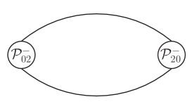
Figure 1: Leading-order vacuum bubble for a free scalar in light-front quantization that includes interactions ${\cal P}^{-}_{02}$ and ${\cal P}^{-}_{20}$ defined in Eqs. (22) and (23) of the text.

Various models can be considered for $\delta_{\epsilon}$, such as the following:

$$\delta_{\epsilon}(p)=\frac{1}{2\epsilon}e^{-p/\epsilon},\;\;\delta_{\epsilon}(p)=\frac{1}{\epsilon\sqrt{\pi}}e^{-p^{2}/\epsilon^{2}},\;\;\mbox{and}\;\;\delta_{\epsilon}(p)=\frac{1}{2\epsilon}\theta(\epsilon-p).$$ (35)

Each is normalized such that $\int_{0}^{\infty}dp\,\delta_{\epsilon}(p)=\frac{1}{2}$, consistent with a limit to $\delta(p)$. Many intermediate quantities will be model dependent but results for physical states will not.

The contribution of the one-loop vacuum bubble is proportional to $\int_{0}^{\infty}dQ\delta_{\epsilon}(Q)^{2}$, as in Eq. (34). Given that $\delta(0)=L/4\pi$ in a finite one-dimensional LF volume $L$ in the $x^{-}$ direction, setting $\int_{0}^{\infty}dQ\delta_{\epsilon}(Q)^{2}\rightarrow\frac{1}{2}\delta(0)\rightarrow L/8\pi$ provides a direct link between the width parameter $\epsilon$ and the volume scale $L$. For the exponential, Gaussian, and step models listed above, we have $\pi/L$, $\sqrt{8\pi}/L$, and $2\pi/L$, respectively, for $\epsilon$ from direct computation of $\int_{0}^{\infty}dQ\delta_{\epsilon}(Q)^{2}$.

A nonperturbative solution for the vacuum can be found in the form of a Fock-state expansion in these ephemeral modes

$$|{\rm vac}\rangle=\sum_{n\,{\rm even}}\int\prod_{i}^{n}dp_{i}\delta_{\epsilon}(\sum^{n}p_{i})\frac{c_{n}}{\sqrt{\prod_{i}^{n}p_{i}}\sum_{i}^{n}\frac{1}{p_{i}}}\frac{1}{\sqrt{n!}}\prod_{i}^{n}a^{\dagger}(p_{i})|0\rangle.$$ (36)

The width of the delta-function replacement $\delta_{\epsilon}$ limits significant contributions to be near zero. The specific momentum dependence included in place of $\psi^{(n)}$ is extrapolated from the perturbative solution for $\psi^{(2)}$ in Eq. (31) and provides for finite contributions to the normalization. The triviality of the free vacuum is recovered in the limit that $\epsilon\rightarrow 0$ and the ephemeral modes are removed.

The vacuum is normalized to 1:

$$1=\langle{\rm vac}|{\rm vac}\rangle=\sum_{n}\int\prod_{i}^{n}dp_{i}\delta_{\epsilon}(\sum_{i}^{n}p_{i})^{2}\frac{|c_{n}|^{2}}{\prod_{i}^{n}p_{i}\left(\sum_{i}^{n}\frac{1}{p_{i}}\right)^{2}}.$$ (37)

This can be simplified by changing the integration variables from $p_{i}$ to $Q\equiv\sum_{i}^{n}p_{i}$ and $x_{i}\equiv p_{i}/Q$, with the constraint that $\sum_{i}^{n}x_{i}=1$. The Jacobian of the transformation is just $Q^{n-1}$, and the vacuum normalization reduces to

$$1=\int Q\delta_{\epsilon}(Q)^{2}dQ\sum_{n}\int\prod_{i}^{n}dx_{i}\delta(1-\sum_{i}^{n}x_{i})\frac{|c_{n}|^{2}}{\prod_{i}^{n}x_{i}\left(\sum_{i}^{n}\frac{1}{x_{i}}\right)^{2}}.$$ (38)

The leading integral over $Q$, which has been factored out, is model dependent but finite. The integrals over $x_{i}$ have mildly singular integrands but are integrable, though not to a closed form; they are best estimated by adaptive multidimensional Monte Carlo methods [38].

To obtain equations for the coefficients $c_{n}$, we project ${\cal P}^{-}_{0}|{\rm vac}\rangle=P_{\rm vac}^{-}|{\rm vac}\rangle$ onto $\int\prod_{i}^{m}\frac{dq_{i}\,\delta_{\epsilon}(\sum_{i}^{m}q_{i})}{\sqrt{\prod_{i}^{m}q_{i}}\sum_{i}^{m}\frac{1}{q_{i}}}\frac{1}{m!}\prod_{i}^{m}a^{\dagger}(q_{i})|0\rangle$, which yields

$$\mu^{2}\int\frac{\prod_{i}^{m}dq_{i}\delta_{\epsilon}(\sum_{i}^{m}q_{i})^{2}}{\left(\prod_{i}^{m}q_{i}\right)\left(\sum_{i}^{m}\frac{1}{q_{i}}\right)}c_{m}$$

$$+\frac{\mu^{2}}{2}\sqrt{m(m-1)}\int\frac{\prod_{i}^{m}dq_{i}\delta_{\epsilon}(\sum_{i}^{m}q_{i})\delta_{\epsilon}(\sum_{i}^{m-2}q_{i})\delta_{\epsilon}(q_{m-1}+q_{m})}{\left(\prod_{i}^{m}q_{i}\right)\left(\sum_{i}^{m}\frac{1}{q_{i}}\right)\left(\sum_{i}^{m-2}\frac{1}{q_{i}}\right)}c_{m-2}$$

$$+\frac{\mu^{2}}{2}\sqrt{(m+2)(m+1)}\int\frac{\prod_{i}^{m}dq_{i}\delta_{\epsilon}(\sum_{i}^{m}q_{i})}{\left(\prod_{i}^{m}q_{i}\right)\sum_{i}^{m}\frac{1}{q_{i}}}$$

$$\rule{36.135pt}{0.0pt}\times\int\frac{dp^{\prime}_{1}dp^{\prime}_{2}\delta_{\epsilon}(p^{\prime}_{1}+p^{\prime}_{2})\delta_{\epsilon}(\sum_{i}^{m}q_{i}+p^{\prime}_{1}+p^{\prime}_{2})}{p^{\prime}_{1}p^{\prime}_{2}\left(\sum_{i}^{m}\frac{1}{q_{i}}+\frac{1}{p^{\prime}_{1}}+\frac{1}{p^{\prime}_{2}}\right)}c_{m+2}$$

$$=P_{\rm vac}^{-}\int\frac{\prod_{i}^{m}dq_{i}\delta_{\epsilon}(\sum_{i}^{m}q_{i})^{2}}{\left(\prod_{i}^{m}q_{i}\right)\left(\sum_{i}^{m}\frac{1}{q_{i}}\right)^{2}}c_{m}.$$

In each term we define $Q$ to be the most extensive sum over momenta; this is $Q=\sum_{i}^{m}q_{i}$ in the first and second terms, as well as the right-hand side, and $Q=\sum_{i}^{m}q_{i}+p^{\prime}_{1}+p^{\prime}_{2}$ in the third term. The individual momenta are then written in terms of fractions $x_{i}=q_{i}/Q$ and $x_{m+j}=p^{\prime}_{j}/Q$. With these new variables, the system of equations becomes

$$\mu^{2}\int\delta_{\epsilon}(Q)^{2}dQ\int\frac{\prod_{i}^{m}dq_{i}\delta(1-\sum_{i}^{m}x_{i})}{\left(\prod_{i}^{m}x_{i}\right)\left(\sum_{i}^{m}\frac{1}{x_{i}}\right)}c_{m}$$

$$+\frac{\mu^{2}}{2}\sqrt{m(m-1)}\int Q\delta_{\epsilon}(Q)dQ$$

$$\rule{36.135pt}{0.0pt}\times\int\frac{\prod_{i}^{m}dx_{i}\delta(1-\sum_{i}^{m}x_{i})\delta_{\epsilon}(Q\sum_{i}^{m-2}x_{i})\delta_{\epsilon}(Q(x_{m-1}+x_{m}))}{\left(\prod_{i}^{m}x_{i}\right)\left(\sum_{i}^{m}\frac{1}{x_{i}}\right)\left(\sum_{i}^{m-2}\frac{1}{x_{i}}\right)}c_{m-2}$$

$$+\frac{\mu^{2}}{2}\sqrt{(m+2)(m+1)}\int Q\delta_{\epsilon}(Q)dQ$$

$$\rule{36.135pt}{0.0pt}\times\int\frac{\prod_{i}^{m+2}dx_{i}\delta(1-\sum_{i}^{m+2}x_{i})\delta_{\epsilon}(Q\sum_{i}^{m}x_{i})\delta_{\epsilon}(Q(x_{m+1}+x_{m}))}{\left(\prod_{i}^{m+2}x_{i}\right)\left(\sum_{i}^{m}\frac{1}{x_{i}}\right)\left(\sum_{i}^{m+2}\frac{1}{x_{i}}\right)}c_{m+2}$$

$$=P_{\rm vac}^{-}\int Q\delta_{\epsilon}(Q)^{2}dQ\int\frac{\prod_{i}^{m}dx_{i}\delta(1-\sum_{i}^{m}x_{i})}{\left(\prod_{i}^{m}x_{i}\right)\left(\sum_{i}^{m}\frac{1}{x_{i}}\right)^{2}}c_{m}.$$

The integrals over $Q$ are model dependent, but, if a model has $\epsilon$ as the only momentum scale, as is the case for the models quoted above, the $\epsilon$ dependence can be factored. For any such model we can define the following three $\epsilon$-independent quantities:

$$\alpha \equiv \epsilon\int\delta_{\epsilon}(Q)^{2}dQ,\;\;\beta\equiv\int Q\delta_{\epsilon}(Q)^{2}dQ,$$ (41)

$$\mbox{and}\;\;\gamma(y) \equiv \frac{\epsilon}{\alpha}\int Q\delta_{\epsilon}(Q)\delta_{\epsilon}(yQ)\delta_{\epsilon}((1-y)Q)dQ.$$

For the exponential, Gaussian, and step models listed above, $\gamma(y)$ is 1/4, $1/[\pi\sqrt{2}(1-y+y^{2})]$, and 1/4, respectively, with $0<y<1$.

The scaling with $\epsilon$ is then clearly such that $P_{\rm vac}^{-}\propto 1/\epsilon$ because each term on the left in Eq. (3.1) is proportional to $\alpha/\epsilon$. We can thus introduce a dimensionless eigenvalue $\eta$ via

$$\eta\equiv\frac{\epsilon}{\mu^{2}}\frac{\beta}{\alpha}P_{\rm vac}^{-}$$ (42)

The system of equations then becomes

$$\int\frac{\prod_{i}^{m}dx_{i}\delta(1-\sum_{i}^{m}x_{i})}{\left(\prod_{i}^{m}x_{i}\right)\left(\sum_{i}^{m}\frac{1}{x_{i}}\right)}c_{m}$$

$$+\frac{1}{2}\sqrt{m(m-1)}\int\frac{\prod_{i}^{m}dx_{i}\delta(1-\sum_{i}^{m}x_{i})\gamma(\sum_{i}^{m-2}x_{i})}{\left(\prod_{i}^{m}x_{i}\right)\left(\sum_{i}^{m}\frac{1}{x_{i}}\right)\left(\sum_{i}^{m-2}\frac{1}{x_{i}}\right)}c_{m-2}$$

$$+\frac{1}{2}\sqrt{(m+2)(m+1)}\int\frac{\prod_{i}^{m+2}dx_{i}\delta(1-\sum_{i}^{m+2}x_{i})\gamma(\sum_{i}^{m}x_{i})}{\left(\prod_{i}^{m+2}x_{i}\right)\left(\sum_{i}^{m}\frac{1}{x_{i}}\right)\left(\sum_{i}^{m+2}\frac{1}{x_{i}}\right)}c_{m+2}$$

$$=\eta\int\frac{\prod_{i}^{m}dx_{i}\delta(1-\sum_{i}^{m}x_{i})}{\left(\prod_{i}^{m}x_{i}\right)\left(\sum_{i}^{m}\frac{1}{x_{i}}\right)^{2}}c_{m},$$

with the dependence on $\gamma$, defined in Eq. (41), the only remaining model dependence. This of course implies that $\eta$ is model dependent; however, model dependence in the vacuum energy is not a concern because it is always subtracted.

As shown earlier, the momentum scale $\epsilon$ for the ephemeral modes is inversely proportional to the one-dimensional volume $L$. For the integral that defines $\alpha$ in Eq. (41), we find $\alpha=\epsilon L/8\pi$ or

$$\epsilon=8\pi\alpha/L$$ (44)

as a model-dependent definition of $\epsilon$ relative to a common length scale. This also shows that $P_{\rm vac}^{-}$ is proportional to the one-dimensional volume and admits a finite vacuum energy density $P_{\rm vac}^{-}/L$.

A state with nonzero momentum can be created from the vacuum with a single creation operator

$$|P\rangle=a^{\dagger}(P)|{\rm vac}\rangle.$$ (45)

It is an eigenstate of ${\cal P}^{-}_{0}$ with eigenvalue $\mu^{2}/P+P_{\rm vac}^{-}$, provided that $P\gg\epsilon$, because we can write

$${\cal P}^{-}_{0}a^{\dagger}(P)|{\rm vac}\rangle = [{\cal P}^{-}_{0},a^{\dagger}(P)]|{\rm vac}\rangle+a^{\dagger}(P){\cal P}^{-}_{0}|{\rm vac}\rangle$$

$$= \left[\frac{\mu^{2}}{P}a^{\dagger}(P)+\frac{\mu^{2}}{2}\int\frac{dp}{\sqrt{pP}}\delta_{\epsilon}(p+P)a(p)\right]|{\rm vac}\rangle+P_{\rm vac}^{-}a^{\dagger}(P)|{\rm vac}\rangle.$$

The second term in the square bracket does not contribute, given the difference in scales between the physical and ephemeral modes, leaving the expected eigenvalue.

3.2 Shifted scalar

If we introduce a shift in the field $\phi$ by an amount $v$, the Lagrangian becomes

$${\cal L}={\cal L}_{v=0}-\mu^{2}v\phi-\frac{1}{2}\mu^{2}v^{2},$$ (47)

and the Hamiltonian is ${\cal P}^{-}={\cal P}^{-}_{0}+{\cal P}^{-}_{\rm int}$, with

$${\cal P}^{-}_{\rm int}=\int dx^{-}[\mu^{2}v\phi+\frac{1}{2}\mu^{2}v^{2}]=\sqrt{4\pi}\mu^{2}v\int\frac{dp}{\sqrt{p}}\delta_{\epsilon}(p)[a(p)+a^{\dagger}(p)]+\frac{1}{2}\mu^{2}v^{2}L.$$ (48)

The standard LF neglect of terms with only creation or annihilation operators would mean that the impact of the shift is lost except for the constant term. We have instead introduced the regulated delta function $\delta_{\epsilon}$ to retain all terms.

The lowest eigenstate of ${\cal P}^{-}$ is the shifted vacuum state $|{\rm vac}\rangle_{v}$:

$$\left({\cal P}^{-}_{0}+{\cal P}^{-}_{\rm int}\right)|{\rm vac}\rangle_{v}=P_{\rm vac}^{-}|{\rm vac}\rangle_{v}.$$ (49)

To incorporate this shift, we define [24] an exponentiated operator

$$B\equiv v\int dp\sqrt{4\pi p}\,\delta_{\epsilon}(p)[a^{\dagger}(p)-a(p)].$$ (50)

which shifts the field $\phi$

$$e^{B}\phi(x^{-})e^{-B}=\phi(x^{-})+v.$$ (51)

When applied to the free Hamiltonian it generates the interaction:

$$e^{B}{\cal P}^{-}_{0}e^{-B}=\int dx^{-}e^{B}\frac{1}{2}\mu^{2}\phi^{2}e^{-B}={\cal P}^{-}_{0}+{\cal P}^{-}_{\rm int}.$$ (52)

It also alters the free vacuum to the shifted vacuum with

$$|{\rm vac}\rangle_{v}=e^{B}|{\rm vac}\rangle$$ (53)

and normalization

$${}_{v}\langle{\rm vac}|{\rm vac}\rangle_{v}=\langle{\rm vac}|e^{B^{\dagger}}e^{B}|{\rm vac}\rangle=\langle{\rm vac}|e^{-B}e^{B}|{\rm vac}\rangle=\langle{\rm vac}|{\rm vac}\rangle=1.$$ (54)

The shifted vacuum $|{\rm vac}\rangle_{v}$ is the eigenstate because

$$\left({\cal P}^{-}_{0}+{\cal P}^{-}_{\rm int}\right)|{\rm vac}\rangle_{v}=e^{B}{\cal P}^{-}_{0}e^{-B}e^{B}|{\rm vac}\rangle=e^{B}{\cal P}^{-}_{0}|{\rm vac}\rangle=P_{\rm vac}^{-}e^{B}|{\rm vac}\rangle=P_{\rm vac}^{-}|{\rm vac}\rangle_{v}.$$ (55)

The vacuum expectation value of the field is

$${}_{v}\langle{\rm vac}|\phi(x^{-})|{\rm vac}\rangle_{v} = \langle{\rm vac}|e^{B^{\dagger}}\phi(x^{-})e^{B}|{\rm vac}\rangle=\langle{\rm vac}|e^{-B}\phi(x^{-})e^{B}|{\rm vac}\rangle$$ (56)

$$= \langle{\rm vac}|(\phi(x^{-})-v)|{\rm vac}\rangle=-v,$$

which restores the shift.

This shows that incorporation of ephemeral modes allows LF quantization to replicate the known results for a shifted scalar field. In the limit that the regulator $\epsilon$ goes to zero, the ephemeral modes are removed but only at the end of the calculation.

3.3 $\phi^{4}$ theory

The Lagrangian for two-dimensional $\phi^{4}$ theory is

$${\cal L}=\frac{1}{2}(\partial_{\mu}\phi)^{2}-\frac{1}{2}\mu^{2}\phi^{2}-\frac{\lambda}{4!}\phi^{4},$$ (57)

where $\lambda$ is the coupling constant. The LF Hamiltonian density is

$${\cal H}=\frac{1}{2}\mu^{2}\phi^{2}+\frac{\lambda}{4!}\phi^{4}.$$ (58)

The LF Hamiltonian ${\cal P}^{-}={\cal P}^{-}_{0}+{\cal P}^{-}_{\rm int}$ then has several terms arising from the interaction ${\cal P}^{-}_{\rm int}={\cal P}^{-}_{04}+{\cal P}^{-}_{40}+{\cal P}^{-}_{22}+{\cal P}^{-}_{13}+{\cal P}^{-}_{31}$ given by

$${\cal P}^{-}_{04} = \frac{\lambda}{24}\int\frac{dp_{1}dp_{2}dp_{3}dp_{4}}{4\pi\sqrt{p_{1}p_{2}p_{3}p_{4}}}\delta_{\epsilon}(\sum_{i}^{4}p_{i})a(p_{1})a(p_{2})a(p_{3})a(p_{4}),$$ (59)

$${\cal P}^{-}_{40} = \frac{\lambda}{24}\int\frac{dp_{1}dp_{2}dp_{3}dp_{4}}{4\pi\sqrt{p_{1}p_{2}p_{3}p_{4}}}\delta_{\epsilon}(\sum_{i}^{4}p_{i})a^{\dagger}(p_{1})a^{\dagger}(p_{2})a^{\dagger}(p_{3})a^{\dagger}(p_{4}),$$ (60)

$${\cal P}^{-}_{22} = \frac{\lambda}{4}\int\frac{dp_{1}dp_{2}}{4\pi\sqrt{p_{1}p_{2}}}\int\frac{dp^{\prime}_{1}dp^{\prime}_{2}}{\sqrt{p^{\prime}_{1}p^{\prime}_{2}}}\delta(p_{1}+p_{2}-p^{\prime}_{1}-p^{\prime}_{2})$$

$$\rule{144.54pt}{0.0pt}\times a^{\dagger}(p_{1})a^{\dagger}(p_{2})a(p^{\prime}_{1})a(p^{\prime}_{2}),$$

$${\cal P}^{-}_{13} = \frac{\lambda}{6}\int\frac{dp_{1}dp_{2}dp_{3}}{4\pi\sqrt{p_{1}p_{2}p_{3}(p_{1}+p_{2}+p_{3})}}a^{\dagger}(p_{1}+p_{2}+p_{3})a(p_{1})a(p_{2})a(p_{3}),$$ (62)

$${\cal P}^{-}_{31} = \frac{\lambda}{6}\int\frac{dp_{1}dp_{2}dp_{3}}{4\pi\sqrt{p_{1}p_{2}p_{3}(p_{1}+p_{2}+p_{3})}}a^{\dagger}(p_{1})a^{\dagger}(p_{2})a^{\dagger}(p_{3})a(p_{1}+p_{2}+p_{3}).$$ (63)

As in the free case, the subscripts represent the number of creation and annihilation operators in each term. Those interaction terms with only creation or only annihilation operators, written as ${\cal P}^{-}_{04}$ and ${\cal P}^{-}_{40}$, are those dropped in standard LF calculations and here have been regulated with $\delta_{\epsilon}$.

The vacuum $|{\rm vac}\rangle_{\lambda}$ is the lowest eigenstate of ${\cal P}^{-}$ with zero LF momentum: ${\cal P}^{-}|{\rm vac}\rangle_{\lambda}=P_{\rm vac}^{-}(\lambda)|{\rm vac}\rangle_{\lambda}$. The expansion in ephemeral modes takes the same form as in Eq. (36), and the system of equations for the coefficients, derived in the same manner as in the free case, becomes

$$\int\frac{\prod_{i}^{m}dx_{i}\delta(1-\sum_{i}^{m}x_{i})}{\left(\prod_{i}^{m}x_{i}\right)\left(\sum_{i}^{m}\frac{1}{x_{i}}\right)}c_{m}$$

$$+\frac{1}{2}\sqrt{m(m-1)}\int\frac{\prod_{i}^{m}dx_{i}\delta(1-\sum_{i}^{m}x_{i})\gamma(\sum_{i}^{m-2}x_{i})}{\left(\prod_{i}^{m}x_{i}\right)\left(\sum_{i}^{m}\frac{1}{x_{i}}\right)\left(\sum_{i}^{m-2}\frac{1}{x_{i}}\right)}c_{m-2}$$

$$+\frac{1}{2}\sqrt{(m+2)(m+1)}\int\frac{\prod_{i}^{m+2}dx_{i}\delta(1-\sum_{i}^{m+2}x_{i})\gamma(\sum_{i}^{m}x_{i})}{\left(\prod_{i}^{m+2}x_{i}\right)\left(\sum_{i}^{m}\frac{1}{x_{i}}\right)\left(\sum_{i}^{m+2}\frac{1}{x_{i}}\right)}c_{m+2}$$

$$+\frac{g}{24}\sqrt{m(m-1)(m-2)(m-3)}\int\frac{\prod_{i}^{m}dx_{i}\delta(1-\sum_{i}^{m}x_{i})\gamma(\sum_{i}^{m-4}x_{i})}{\left(\prod_{i}^{m}x_{i}\right)\left(\sum_{i}^{m}\frac{1}{x_{i}}\right)\left(\sum_{i}^{m-4}\frac{1}{x_{i}}\right)}c_{m-4}$$

$$+\frac{g}{24}\sqrt{(m+4)(m+3)(m+2)(m+1)}\int\frac{\prod_{i}^{m+4}dx_{i}\delta(1-\sum_{i}^{m+4}x_{i})\gamma(\sum_{i}^{m}x_{i})}{\left(\prod_{i}^{m+4}x_{i}\right)\left(\sum_{i}^{m}\frac{1}{x_{i}}\right)\left(\sum_{i}^{m+4}\frac{1}{x_{i}}\right)}c_{m+4}$$

$$+\frac{g}{4}m\sqrt{m-1}\int\frac{\prod_{i}^{m}dx_{i}\delta(1-\sum_{i}^{m}x_{i})dx^{\prime}_{1}dx^{\prime}_{2}\delta(x^{\prime}_{1}+x^{\prime}_{2}-x_{m-1}-x_{m})}{\left(\prod_{i}^{m}x_{i}\right)x^{\prime}_{1}x^{\prime}_{2}\left(\sum_{i}^{m}\frac{1}{x_{i}}\right)\left(\sum_{i}^{m-2}\frac{1}{x_{i}}+\frac{1}{x^{\prime}_{1}}+\frac{1}{x^{\prime}_{2}}\right)}c_{m}$$

$$+\frac{g}{6}(m-2)\sqrt{m(m-1)}\int\frac{\prod_{i}^{m}dx_{i}\delta(1-\sum_{i}^{m}x_{i})}{\left(\prod_{i}^{m}x_{i}\right)\left(\sum_{m-2}^{m}x_{i}\right)\left(\sum_{i}^{m}\frac{1}{x_{i}}\right)\left(\sum_{i}^{m-3}\frac{1}{x_{i}}+\frac{1}{\sum_{m-2}^{m}x_{i}}\right)}c_{m-2}$$

$$+\frac{g}{6}m\sqrt{(m+2)(m+1)}\int\frac{\prod_{i}^{m}dx_{i}\delta(1-\sum_{i}^{m}x_{i})\prod_{i}^{3}dx^{\prime}_{i}\delta(\sum_{i}^{3}x^{\prime}_{i}-x_{m})}{\left(\prod_{i}^{m}x_{i}\right)\left(\prod_{i}^{3}x^{\prime}_{i}\right)\left(\sum_{i}^{m}\frac{1}{x_{i}}\right)\left(\sum_{i}^{m-1}\frac{1}{x_{i}}+\sum_{i}^{3}\frac{1}{x^{\prime}_{i}}\right)}c_{m+2}$$

$$=\eta(\lambda)\int\frac{\prod_{i}^{m}dx_{i}\delta(1-\sum_{i}^{m}x_{i})}{\left(\prod_{i}^{m}x_{i}\right)\left(\sum_{i}^{m}\frac{1}{x_{i}}\right)^{2}}c_{m},$$

with $g=\lambda/4\pi\mu^{2}$ as a dimensionless coupling constant. The dimensionful eigenenergy is $P_{\rm vac}^{-}(\lambda)=\frac{\mu^{2}}{\epsilon}\frac{\alpha}{\beta}\eta(\lambda)$. The quantities $\alpha$ and $\beta$ and the function $\gamma$ are defined as before in Eq. (41).

States with nonzero momentum are again built on this vacuum; however, with the interaction present they are of course not as simple as the free case and instead have their own Fock state expansion

$$|P\rangle=\sum_{n}\Psi_{n}^{\dagger}(P)|{\rm vac}\rangle_{\lambda},$$ (65)

with

$$\Psi_{n}^{\dagger}(P)\equiv\int\prod_{i}^{n}dp_{i}\delta(\sum_{i}^{n}p_{i}-P)\psi_{n}(p_{i})\frac{1}{\sqrt{n!}}\prod_{i}^{n}a^{\dagger}(p_{i}).$$ (66)

Such a state is to satisfy the eigenvalue problem

$${\cal P}^{-}|P\rangle=\left[\frac{M^{2}}{P}+P_{\rm vac}^{-}(\lambda)\right]|P\rangle.$$ (67)

This will cause some mixing between physical and ephemeral modes as the wave functions $\psi_{n}$ extend to zero momentum with a nominal behavior of

$$\psi_{n}(p_{i})\sim\frac{1}{\left(\sqrt{\prod_{i}^{n}p_{i}}\right)\left(\sum_{i}^{n}\frac{1}{p_{i}}\right)}.$$ (68)

The mixing will introduce tadpole contributions that are absent from a standard LF calculation. There are also vacuum bubble contributions when the physical and ephemeral modes do not mix, but these bubbles contribute only to $P_{\rm vac}^{-}(\lambda)$ and are subtracted. For a graphical representation of the lowest order contributions, see Fig. 2.

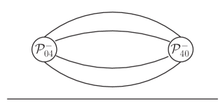
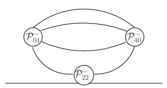
(a)	(b)
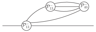
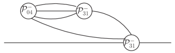
(c)	(d)

Figure 2: Lowest-order vacuum bubble (a) and tadpole graphs (b), (c), and (d) in $\phi^{4}$ theory. The vertices are labeled with the associated Hamiltonian term.

These contributions can be seen explicitly in perturbation theory [24]. If only perturbations due to ${\cal P}^{-}_{04}$, ${\cal P}^{-}_{40}$, and ${\cal P}^{-}_{22}$ are kept, the equations for the lowest order Fock-state wave functions become

$$\frac{\mu^{2}}{P}\psi_{1} + \frac{\lambda}{\sqrt{24}}\int\frac{\prod_{i}^{4}dp_{i}}{4\pi\sqrt{\prod_{i}^{4}p_{i}}}\delta_{\epsilon}(\sum_{i}^{4}p_{i})\psi_{5}(p_{1},\ldots,p_{5})$$

$$=\left(\frac{M^{2}}{P}+P_{\rm vac}^{-}\right)\psi_{1},$$

$$\left(\sum_{i}^{5}\frac{\mu^{2}}{p_{i}}\right)\psi_{5} + \frac{\lambda}{24}\frac{1}{5}\left[\frac{\delta_{\epsilon}(\sum_{i}^{4}p_{i})}{4\pi\sqrt{\prod_{i}^{4}p_{i}}}+(p_{5}\leftrightarrow p_{1},p_{2},p_{3},p_{4})\right]\psi_{1}$$

$$+ 20\frac{\lambda}{4}\int\frac{dp^{\prime}_{1}dp^{\prime}_{2}}{4\pi\sqrt{p_{1}p_{2}p^{\prime}_{1}p^{\prime}_{2}}}\delta(p_{1}+p_{2}-p^{\prime}_{1}-p^{\prime}_{2})\psi_{5}(p^{\prime}_{1},p^{\prime}_{2},p_{3},p_{4},p_{5})=\frac{M^{2}}{P}\psi_{5}.$$

The second equation can be solved approximately by iteration of the self interaction to first order in $\lambda$. Substitution of the $\psi_{5}$ obtained by this approximation into the first equation yields two contributions. One corresponds to the bubble in Fig. 2(a) and contributes the following to $P_{\rm vac}^{-}$ [24]:

$$-\frac{\lambda^{2}}{\mu^{2}}\int\delta_{\epsilon}(Q)^{2}dQ\int\frac{\prod_{i}^{4}dx_{i}}{\prod_{i}^{4}x_{i}}\delta(1-\sum_{i}^{4}x_{i}),$$ (71)

which diverges as $1/\epsilon\sim L$. The other corresponds to Fig. 2(b) and contributes the following to $M^{2}/P$ [24]:

$$\frac{\lambda^{3}}{P}\int\delta_{\epsilon}(Q)dQ\int\frac{\prod_{i}^{4}dx_{i}}{(\prod_{i}^{4}x_{i})x_{4}\left(\sum_{i}^{4}\frac{\mu^{2}}{x_{i}}\right)^{2}}.$$ (72)

This is finite and has the correct dependence on the total LF momentum for a self-energy correction. Figures 2(c) and (d) also contribute when ${\cal P}^{-}_{13}$ and ${\cal P}^{-}_{31}$ are also kept.

The solutions of the vacuum problem stated in Eq. (3.3) and the physical-state problem in Eq. (67) will provide for a finite mass value after the vacuum subtraction and for physical Fock-state wave functions that can be used to compute expectation values. This will allow investigation of the critical coupling, where states with odd and even numbers of constituents become degenerate and mix, which allows the field $\phi$ to have a nonzero expectation value.

Another, related approach is that of the light-front coupled-cluster (LFCC) method [49]. Ephemeral modes can be included [50] by building the vacuum as a generalized coherent state [51, 52].

4 Summary

Zero modes have important roles to play in the structure of light-front field theories and their solutions. In particular, the LF vacuum is not completely trivial. Zero modes and the near-zero ephemeral modes act to induce effects that are otherwise missing from LF calculations. Although for many LF calculations these effects are not important, complete consistency with equal-time calculations cannot be achieved without zero modes.

With regard to the specifics of zero-mode effects, there are various calculations still to be done, to fully understand the mechanisms of zero modes and ephemeral modes. For zero modes within DLCQ, the perturbative approach to the constraint equation and the subsequent construction of the effective Hamiltonian, to include zero-mode loops, should be carried out and used to study the impact of the added effective interactions on the spectrum of two-dimensional $\phi^{4}$ theory and on its symmetry breaking. Similarly, the renormalization of the nonperturbative approach should be systematized, so that many-body calculations can be attempted.

A better understanding of vacuum to vacuum transitions is also needed. Tadpoles clearly make an important contribution to equivalence with equal-time calculations, as do vacuum bubbles. Light-front calculations that include them will be central to understanding symmetry breaking. Two-dimensional $\phi^{4}$ theory is again an ideal model to consider.

Inclusion of tadpoles has already been shown to resolve a disagreement with equal-time calculations [22], but this was not done from within a calculation that was exclusively light-front. Instead, we have proposed [24] a fundamental reinterpretation of light-front Hamiltonians to include vacuum to vacuum transitions in a way that calculations can be done strictly within the light-front framework.

Acknowledgements

This work was supported in part by the Minnesota Supercomputing Institute and the Research Computing and Data Services at the University of Idaho through grants of computing time.

Declarations

• Funding: The work on zero modes in DLCQ by perturbation in the resolution [37] was funded by the US Department of Energy, under Contract No. DE-FG02-98ER41087.

• Conflict of interest: Not applicable.

• Ethics approval and consent to participate: Not applicable.

• Consent for publication: Institutional consent not required.

• Data availability: Not applicable.

• Materials availability: Not applicable.

• Code availability: Not applicable.

• Author contribution: Both authors contributed equally to the work, and read and agreed to the manuscript submitted for publication.

References

- [1] Dirac, P.A.M.: Forms of relativistic dynamics, Rev. Mod. Phys. 21, 392-399 (1949)
- [2] Brodsky, S.J., Pauli, H.-C., Pinsky, S.S.: Quantum chromodynamics and other field theories on the light cone. Phys. Rep. 301, 299-486 (1998)
- [3] Carbonell, J., Desplanques, B., Karmanov, V.A., Mathiot, J.F.: Explicitly covariant light front dynamics and relativistic few body systems. Phys. Rep. 300, 215-347 (1998)
- [4] Miller, G.A.: Light front quantization: A technique for relativistic and realistic nuclear physics. Prog. Part. Nucl. Phys. 45, 83-155 (2000).
- [5] Heinzl, T.: Light cone quantization: Foundations and applications. Lect. Notes Phys. 572, 55-142 (2001)
- [6] Burkardt, M.: Light front quantization, Adv. Nucl. Phys. 23, 1-74 (2002)
- [7] Hiller, J.R.: Nonperturbative light-front Hamiltonian methods. Prog. Part. Nucl. Phys. 90, 75-124 (2016)
-
[8]
Burkardt, M., Lenz, F., Thies, M.:
Chiral condensate and short time evolution of QCD(1+1) on the light cone.
Phys. Rev. D 65, 125002 (2002)
Lenz, F., Ohta, K., Thies, M., Yazaki, K.: Chiral symmetry in light cone field theory. Phys. Rev. D 70, 025015 (2004)
Beane, S.R.: Broken chiral symmetry on a null plane. Ann. Phys. 337, 111-142 (2013) -
[9]
Heinzl, T., Krusche, S., Werner, E.:
Spontaneous symmetry breaking in light cone quantum field theory.
Phys. Lett. B 272, 54-60 (1991)
Heinzl, T., Stern, C., Werner, E., Zellermann, B.: The vacuum structure of light front in -dimensions theory. Z. Phys. C 72, 353-364 (1996) -
[10]
Robertson, D.G.:
On spontaneous symmetry breaking in discretized light cone field theory.
Phys. Rev. D 47, 2549-2553 (1993)
McCartor, G., Robertson, D.G.: Bosonic zero modes in discretized light cone field theory. Z. Phys. C 53, 679-686 (1992). -
[11]
Bender, C.M., Pinsky, S., van de Sande, B.:
Spontaneous symmetry breaking of in dimensions in light front field theory.
Phys. Rev. D 48, 816-821 (1993)
Pinsky, S.S., van de Sande, B.: Spontaneous symmetry breaking of -dimensional theory in light front field theory. 2. Phys. Rev. D 49, 2001-2013 (1994) - [12] Pinsky, S.S., van de Sande, B., Hiller, J.R.: Spontaneous symmetry breaking of -dimensional theory in light front field theory. 3. Phys. Rev. D 51, 726-733 (1995)
- [13] Tsujimaru, S., Yamawaki, K.: Zero mode and symmetry breaking on the light front. Phys. Rev. D 57, 4942-4964 (1998)
-
[14]
Martinovic, L., Vary, J.P.:
Fermionic zero modes and spontaneous symmetry breaking on the light front.
Phys. Rev. D 64, 105016 (2001)
Martinovic, L.: Spontaneous symmetry breaking in light front field theory. Phys. Rev. D 78, 105009 (2008) -
[15]
Aslan, F.P., Burkardt, M.:
Singularities in twist-3 quark distributions.
Phys. Rev. D 101, 016010 (2020)
Ji, X.: Fundamental Properties of the Proton in Light-Front Zero Modes. Nucl. Phys. B 960, 115181 (2020) - [16] Lee, D., Salwen, N.: The diagonalization of quantum field hamiltonians. Phys. Lett. B 503, 223-235 (2001)
- [17] Sugihara, T.: Density matrix renormalization group in a two-dimensional lambda Hamiltonian lattice model. JHEP 05(2004), 007 (2004)
- [18] Schaich, D., Loinaz, W.: An improved lattice measurement of the critical coupling in theory. Phys. Rev. D 79, 056008 (2009)
- [19] Bosetti, P., De Palma, B., Guagnelli, M.: Monte Carlo determination of the critical coupling in theory. Phys. Rev. D 92, 034509 (2015)
- [20] Milsted,A., Haegeman, J., Osborne, T.J.: Matrix product states and variational methods applied to critical quantum field theory. Phys. Rev. D 88, 085030 (2013).
-
[21]
Rychkov, S., Vitale, L.G.:
Hamiltonian truncation study of the theory in two dimensions.
Phys. Rev. D 91, 085011 (2015)
Hamiltonian truncation study of the theory in two dimensions. II: The -broken phase and the Chang duality. Phys. Rev. D 93, 065014 (2016) -
[22]
Burkardt, M., Chabysheva, S.S., Hiller, J.R.:
Two-dimensional light-front theory in a symmetric polynomial basis.
Phys. Rev. D 94, 065006 (2016)
Chabysheva, S.S., Hiller, J.R.: Light-front theory with sector-dependent mass. Phys. Rev. D 95, 096016 (2017) - [23] Vary, J.P., Huang, M., Jawadekar, S., Sharaf, M., Harindranath, A., and Chakrabarti, D.: Critical coupling for two-dimensional theory in discretized light-cone quantization. Phys. Rev. D 105, 016020 (2022)
- [24] Chabysheva, S.S., Hiller, J.R.: Tadpoles and vacuum bubbles in light-front quantization. Phys. Rev. D 105, 116006 (2022)
- [25] Hornbostel, K.: Nontrivial vacua from equal time to the light cone. Phys. Rev. D 45, 3781-3801 (1992)
-
[26]
Ji C.-R., Mitchell, C.:
Poincare invariant algebra from instant to light front quantization.
Phys. Rev. D 64, 085013 (2001)
Ji, C.-R., Suzuki, A.T.: Interpolating scattering amplitudes between the instant form and the front form of relativistic dynamics. Phys. Rev. D 87, 065015 (2013) - [27] Chabysheva, S.S., Hiller, J.R.: Transitioning from equal-time to light-front quantization in theory. Phys. Rev. D 102, 116010 (2020)
-
[28]
Burkardt, M.:
Phys. Rev. D 47, 4628 (1993)
Much ado about nothing: Vacuum and renormalization in the light-front framework. Nucl. Phys. A 670, 72-75 (2000)
Light-front quantization of the sine-Gordon model. Phys. Rev. D 47, 4628-4633 (1993) - [29] Mannheim, P.D., Lowdon, P., Brodsky, S.J.: Structure of light front vacuum sector diagrams. Phys. Lett. B 797, 134916 (2019)
- [30] Chang, S.-J., Ma, S.-K.: Feynman rules and quantum electrodynamics at infinite momentum. Phys. Rev. 180, 1506-1513 (1969)
- [31] Yan, T.M.: Quantum field theories in the infinite momentum frame. 4. Scattering matrix of vector and Dirac fields and perturbation theory. Phys. Rev. D 7, 1780-1800 (1973)
-
[32]
Mannheim, P.D.:
Equivalence of light-front quantization and instant-time quantization.
Phys. Rev. D 102, 025020 (2020)
Mannheim, P.D., Lowdon, P., Brodsky, S.J.: Comparing light-front quantization with instant-time quantization. Phys. Rept. 891, 1-65 (2021) - [33] Polyzou, W.N.: Relation between instant and light-front formulations of quantum field theory. Phys. Rev. D 103, 105017 (2021)
- [34] Collins, J.: The non-triviality of the vacuum in light-front quantization: An elementary treatment. arXiv:1801.03960 [hep-ph]
- [35] Martinovic, L., Dorokhov, A.: Vacuum loops in light-front field theory. Phys. Lett. B 811, 135925 (2020)
-
[36]
Pauli, H.-C., Brodsky, S.J.:
Solving field theory in one space one time dimension.
Phys. Rev. D 32, 1993-2000 (1985)
Discretized light cone quantization: Solution to a field theory in one space one time dimension. Phys. Rev. D 32, 2001-2013 (1985) - [37] Chabysheva, S.S., Hiller, J.R.: Zero momentum modes in discrete light-cone quantization. Phys. Rev. D 79, 096012 (2009)
-
[38]
Lepage, G.P.:
Adaptive multidimensional integration: VEGAS enhanced.
J. Comput. Phys. 439, 110386 (2021)
A New Algorithm for Adaptive Multidimensional Integration. J. Comput. Phys. 27, 192-203 (1978) - [39] Simon, B., and Griffiths, R.B.: The field theory as a classical ising model. Commun. Math. Phys. 33, 145-164 (1973)
- [40] Maskawa, T., Yamawaki, K.: The problem of mMode in the null plane field theory and Dirac’s method of quantization. Progr. Theor. Phys. 56, 270-283 (1976)
- [41] Wittman, R.S.: Symmetry breaking in the theory and the light-front vacuum. In: Johnson, M.B., Kisslinger, L.S. (eds.) Nuclear and Particle Physics on the Light Cone, pp. 331-335. World Scientific, Singapore (1989)
- [42] Baym, G.: Inconsistency of cubic boson-boson interactions. Phys. Rev. 117, 886-888 (1960)
- [43] Gross, F., Savkli, C., Tjon, J.: The stability of the scalar interaction. Phys. Rev. D 64, 076008 (2001)
- [44] Rozowsky J.S., Thorn, C.B.: Spontaneous symmetry breaking at infinite momentum without zero modes. Phys. Rev. Lett. 85, 1614-1617 (2000)
- [45] Hellerman, S., Polchinski, J.: Compactification in the lightlike limit. Phys. Rev. D 59, 125002 (1999)
-
[46]
Taniguchi, M., Uehara, S., Yamada, S., Yamawaki, K.:
Does DLCQ S matrix have a covariant continuum limit?.
Mod. Phys. Lett. A 16, 2177-2185 (2001)
Recovering Lorentz invariance of DLCQ. arXiv:hep-th/0309240
Heinzl, T.: Light-cone zero modes revisited. arXiv:hep-th/0310165 -
[47]
McCartor, G.:
Light cone quantization for massless fields.
Z. Phys. C 41, 271-275 (1988)
Heinzl,T., Ilderton, A., Seipt, D.: Mode truncations and scattering in strong fields. Phys. Rev. D 98, 016002 (2018) - [48] Herrmann, M., Polyzou, W.N.: Light-front vacuum. Phys. Rev. D 91, 085043 (2015)
- [49] Chabysheva S.S., Hiller, J.R.: A light-front coupled-cluster method for the nonperturbative solution of quantum field theories. Phys. Lett. B 711, 417-422 (2012)
- [50] Chabysheva S.S., Hiller, J.R.: Zero modes in the light-front coupled-cluster method. Ann. Phys. 340, 188-204 (2014)
- [51] Harindranath, A., and Vary, J.P.: Variational calculation of the spectrum of two-dimensional theory in light-front field theory. Phys. Rev. D 37, 3010–3013 (1988)
-
[52]
Martinovic, L.:
Non-trivial Fock vacuum of the light-front Schwinger model.
Phys. Lett. B 400, 335-340 (1997)
Martinovic, L., Vary, J.P.: Theta-vacuum of the bosonized massive light-front Schwinger model. Phys. Lett. B 459, 186-192 (1999)
Bhamre, D., Gogia, S., Misra, A.: Cancellation of infrared divergences in in the light front coherent state formalism. Phys. Rev. D 111, 016001 (2025)