Choose Your Model Size: Any Compression by a Single Gradient Descent

Abstract

The adoption of Foundation Models in resource-constrained environments remains challenging due to their large size and inference costs. A promising way to overcome these limitations is post-training compression, which aims to balance reduced model size against performance degradation. This work presents Any Compression via Iterative Pruning (ACIP), a novel algorithmic approach to determine a compression-performance trade-off from a single stochastic gradient descent run. To ensure parameter efficiency, we use an SVD-reparametrization of linear layers and iteratively prune their singular values with a sparsity-inducing penalty. The resulting pruning order gives rise to a global parameter ranking that allows us to materialize models of any target size. Importantly, the compressed models exhibit strong predictive downstream performance without the need for costly fine-tuning. We evaluate ACIP on a large selection of open-weight LLMs and tasks, and demonstrate state-of-the-art results compared to existing factorisation-based compression methods. We also show that ACIP seamlessly complements common quantization-based compression techniques.

1 Introduction

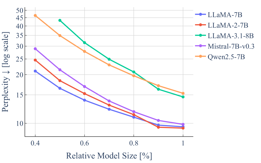
Figure 1: Compression-performance trade-off curves generated by ACIP on C4 for a variety of LLMs. Each curve is obtained by a single gradient descent run and all compressed models can be materialized without recomputation.

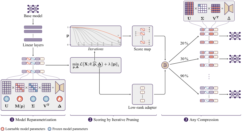
Figure 2: A visual overview of ACIP. The linear layers of the base model are reparametrized in terms of their singular value decomposition $\mathbf{U}\mathbf{M}\boldsymbol{\Sigma}\mathbf{V}^{\top}$​, with a (binary) singular value mask $\mathbf{M}$, and a low-rank adapter $\boldsymbol{\Delta}$. The objective function is optimized over the mask parameters $\mathbf{p}$ and adapters $\boldsymbol{\Delta}$, where sparsity is induced on $\mathbf{p}$ by an $\ell_{1}$-penality leading to pruned entries in the mask $\mathbf{M}$. The optimization path of $\mathbf{p}$ gives rise to a score map that determines the global importance of the singular values across the full model. Potential compression errors are compensated by $\boldsymbol{\Delta}$. Based on the parameter scores, the base model can be flexibly compressed to any target size by masking the entries of $\boldsymbol{\Sigma}$. The learned adapters $\boldsymbol{\Delta}$ are used as correction for any compression level.

Post-training compression of Foundation Models, especially large language models (LLMs), promises access to powerful tools where resources are limited, e.g., in e-commerce, mobile deployments, or on the shop floor. Typical reasons for scarcity include constrained access to hardware, monetary limitations, high inference speed requirements, and environmental concerns (Hohman et al., 2024). However, model compression is not for free — it typically comes with a trade-off between model size and desired downstream performance. In order to support decision-making, it is of fundamental importance to find the right balance between these two objectives. In fact, when deploying large-scale models, questions like the following ones arise:

• I am willing to give up on $X\%$ of model performance, how much can I compress model $Y$?
  My infrastructure allows me to run an $N$ parameter model, what is the best model within this budget?
  What are the minimal hardware requirements for an LLM with a benchmark performance of at least $Z$?

To make model compression more accessible, the algorithmic characterization of the underlying trade-off should be a high priority in the development of new algorithms (Boggust et al., 2025). In the scientific literature, however, this aspect is often secondary, and instead, performance is compared at preset compression levels (Zhu et al., 2024).

Apart from resource-intensive model distillation (Hinton et al., 2015), there are currently two dominating approaches to efficient post-training model compression: (i) model quantization, which limits weight fidelity by reducing numerical precision, and (ii) (un-)structured weight pruning which aims to delete unnecessary or redundant weights from a model (Zhu et al., 2024). While many of these approaches lead to good compression results, they typically allow only for constant compression factors in case of quantization or require specialized hardware, e.g., to implement $n{:}m$-sparsity in unstructured pruning or low-bit representations in quantization. Due to these structural constraints, such methods do not enable a full characterization of the compression-performance trade-off for a given base model.

Inspired by the effectiveness of low-rank adapters in LLMs (Hu et al., 2022), factorization-based compression can be applied without any integral changes to a network’s architecture, by simply reparametrizing linear layers. This particular form of structured pruning allows, in principle, for compression factors on a fine-grained scale without additional hardware constraints. However, the performance of existing algorithms falls behind the above-described compression techniques, so that competitive performance for stronger size-reduction is only achieved with additional fine-tuning (Wang et al., 2024; Yuan et al., 2024; Jaiswal et al., 2024).

In this work, we follow the promising idea of factorization-based compression and find a positive answer to our initial quest:

• Design an efficient compression procedure that algorithmically determines the compression-performance trade-off for a given pre-trained model.

The basic idea of our proposed method, Any Compression via Iterative Pruning (ACIP),​ is to induce sparsity in the singular values of the weight matrices, which leads to low-rank and therefore compressed parametrizations. Instead of layer-wise updates, we rely on a simple end-to-end objective function that is optimized through stochastic gradient descent. Crucially, the optimization trajectory of the pruned singular values gives rise to a score map representing a global importance ranking across all linear network layers. This allows us to materialize compressed models of any target size without additional computation and produce trade-off curves like in Figure 1. See also Figure 2 for a visualization of ACIP and Section 2 for a more detailed description.

We will demonstrate that ACIP satisfies the following practical requirements, which at the same time, also form the key contributions of our work:

Easy-to-Use & Fast

ACIP allows practitioners to compress pre-trained models to any size from a single optimization run. It is parameter-efficient, requires no hyperparameter tuning and no feature engineering due to its end-to-end nature.

Flexible & Complementary

ACIP can be applied to any model that has linear layers as central building blocks without further structural assumptions. It can be used with arbitrary task loss functions and seamlessly complements quantization-based compression approaches.

Effective & Robust

ACIP exhibits state-of-the-art results among factorization-based pruning approaches. It provides consistent and robust compression-performance trade-offs for a variety of popular LLMs and zero-shot evaluation tasks.

Our main results supporting these claims are presented in Section 4. The interested reader is also referred to the supplementary material, where we address some design decisions and conceptual aspects (Appendix A), provide implementation and runtime details (Appendix B), as well as additional experiments (Appendix C and Appendix D).

2 Method

ACIP is an easy-to-use method to build models at any compression rate based on an SVD-weight factorization (Section 2.1.2). We leverage ideas from sparse recovery (Section 2.1.3) to iteratively prune model parameters and then use the resulting pruning order to derive a global importance ranking (Section 2.1.1). With these preliminaries at hand, the algorithmic details of ACIP are formulated in Section 2.2.

2.1 Preliminaries

2.1.1 Score-based Parameter Pruning

As motivated in the introduction, the goal of this work is to determine the compression-performance trade-off of a pre-trained model. To do this, we use score-based parameter pruning, a framework that has been successfully applied to model compression since the 1980s (LeCun et al., 1989; Hassibi et al., 1993). In score-based pruning, a score map $\boldsymbol{\rho}$ is created that assigns an importance score $\rho_{i}$ to all target parameters $\theta_{i}$. Naturally, this approach gives rise to a (global) ranking of parameters that allows for model compression at any desired rate.

There are many ways to design useful score maps. For example, they can be derived based on curvature at a local optimum (LeCun et al., 1989; Hassibi et al., 1993) or by using hand-designed local features (Sun et al., 2024; Frantar & Alistarh, 2023). In Section 2.2.2, we present a novel, data-driven approach to score maps that does not require any handcrafting or feature engineering.

2.1.2 Compressing Linear Layers

This work builds on the compression of the weight matrices in linear layers of a model. These weights typically account for the largest portion of parameters in deep learning models. We consider linear layers of the form

$$\mathbf{y}=\mathbf{W}\mathbf{x}+\mathbf{b},$$ (1)

where $\mathbf{W}$ is a $m\times n$ matrix and $\mathbf{b}$ is a bias term. We aim for a low-rank compression based on a matrix factorization such that

$$\mathbf{y}=\mathbf{P}\mathbf{Q}\mathbf{x}+\mathbf{b},$$ (2)

with $\mathbf{P}$ and $\mathbf{Q}$ being matrices of sizes $m\times k$ and $k\times n$, respectively, where $k\ll\min(m,n)$. The layer parametrization in (2) may be interpreted as a (lossy) compression of the parametrization in (1), leading to a smaller memory footprint whenever $k(m+n)<mn$. Note that matrix factorization can be used to compress the parameters of any linear layer, including dense layers as well as efficiently parametrized layers such as convolutional layers (Idelbayev & Carreira-Perpiñán, 2020). In this work, we focus on the compression of dense layers in transformers (Vaswani et al., 2017).

Singular Value Decomposition

For low-rank factorizations in ACIP, we choose the singular value decomposition (SVD) which has been used extensively in model compression (Idelbayev & Carreira-Perpiñán, 2020; Yuan et al., 2024; Wang et al., 2024). SVD factorizes any $m\times n$ weight matrix $\mathbf{W}_{l}$ of rank $r\leq\min(m,n)$ at layer $l$ as

$$\mathbf{W}_{l}=\mathbf{U}_{l}\boldsymbol{\Sigma}_{l}\mathbf{V}_{l}^{\top},$$ (3)

where $\mathbf{U}_{l}$ and $\mathbf{V}_{l}$ are $m\times r$ and $n\times r$ matrices of (orthonormal) singular vectors, and $\boldsymbol{\Sigma}_{l}$ is a $r\times r$ diagonal matrix containing the singular values $\mathbf{s}_{l}^{(i)}>0$. Note that we have used the compact SVD which ignores the null-space vectors of the full SVD. We may reduce the inner dimension $r$ of the SVD to $k<r$ with

$$\mathbf{W}_{l}\approx\tilde{\mathbf{U}}_{l}\tilde{\boldsymbol{\Sigma}}_{l}\tilde{\mathbf{V}}_{l}^{\top}$$ (4)

by defining $\tilde{\mathbf{U}}_{l}$ and $\tilde{\mathbf{V}}_{l}^{\top}$ to only contain $k$ singular vectors associated with a selected subset of singular values. To preserve the matrix norm of $\mathbf{W}_{l}$, selecting the $k$ largest singular values leads to an optimal approximation of $\mathbf{W}_{l}$ under rank constraints (Mirsky, 1960). It has been previously argued, however, that this approach does not yield satisfactory results in deep learning as is does not take into account the (training) data (Hsu et al., 2022). Different approaches have been presented to address this problem (Hsu et al., 2022; Yuan et al., 2024; Wang et al., 2024; Chen et al., 2021).

2.1.3 $\ell_{1}$-regularization

Consider a generic loss functional $\mathcal{L}(\mathbf{X};\boldsymbol{\theta})$ evaluated on some model that is specified through a parameter vector $\boldsymbol{\theta}$ and data $\mathbf{X}$. During model training, sparsity in $\boldsymbol{\theta}$ is typically encouraged by solving the penalized optimization problem

$$\min_{\boldsymbol{\theta}}\mathcal{L}\bigl{(}\mathbf{X};\boldsymbol{\theta}\bigr{)}+\lambda\left\lVert\boldsymbol{\theta}\right\rVert_{1},\ \quad\lambda>0,$$ (5)

which is known as $\ell_{1}$-regularization, or least absolute shrinkage and selection operator (LASSO) in case of (generalized) linear models (Tibshirani, 1996; Hastie et al., 2015). Feature selection plays a key role in this optimization problem. Consider the solution to (5) as a function of regularization parameter $\lambda$: Increasing $\lambda$ leads to a sparser solution in $\boldsymbol{\theta}$. This effectively gives a ranking of feature importances for the solution of (5) through the so-called regularization path (Tibshirani, 1996; Efron et al., 2004; Mairal & Yu, 2012) — an idea that inspired our approach. Furthermore, previous results indicate that optimization paths of iterative schemes can be related to regularization paths (Suggala et al., 2018). Intuitively, this suggests that general optimization paths of iterative schemes for $\ell_{1}$-objectives reveal information about feature importance in the context of sparse models as well.

In this work, we will successively increase $\lambda$ to introduce a higher degree of model compression in terms of parameter sparsity in a controlled manner (see also Remark 2.1 below).

2.2 Any Compression via Iterative Pruning (ACIP)

We now present Any Compression via Iterative Pruning (ACIP), which consists of the following three key steps:

Step 1. (Model Reparametrization)

Apply SVD to the weights $\mathbf{W}_{l}$ of all (dense) linear layers according to (6), and introduce low-rank adapters and singular value masks as tunable parameters.

Step 2. (Scoring via Iterative Pruning)

Choose a surrogate loss $\mathcal{L}$ and a calibration data set $\mathbf{X}$. Perform iterative pruning of singular values and simultaneous training of low-rank adapters by applying gradient-based optimization as in (8). Obtain a parameter score map $\boldsymbol{\rho}$ by using Algorithm 1.

Step 3. (Any Compression)

Choose any desired compression rate. Use score map $\boldsymbol{\rho}$ and low-rank adapters $\boldsymbol{\Delta}$ to materialize the compressed model.

We provide a more detailed description of these steps in the following. For a visual presentation of ACIP, we refer back to Figure 2.

2.2.1 Step 1. Model Reparametrization

We start by reparametrizing all linear layers of a network using SVD as described in (3) and assign

$$\mathbf{W}_{l}\leftarrow\mathbf{U}_{l}\mathbf{M}_{l}\boldsymbol{\Sigma}_{l}\mathbf{V}_{l}^{\top}+\boldsymbol{\Delta}_{l},$$ (6)

where $\mathbf{M}_{l}$ is a binary diagonal matrix with entries $\mathbf{m}^{(i)}_{l}\in\{0,1\}$ masking the singular values $\mathbf{s}_{l}^{(i)}$ in $\boldsymbol{\Sigma}$, and $\boldsymbol{\Delta}_{l}$ is a low-rank adapter (LoRA) (Hu et al., 2022). We find that the addition of a low-rank adapter helps to compensate for potential errors that are introduced through pruning. We initialize $\mathbf{M}_{l}$ to be the identity matrix and $\boldsymbol{\Delta}_{l}$ to zero weights. In this way, the reparametrized model is initialized to be identical to the original model up to numerical precision.

We assign the binary masks $\mathbf{m}_{l}^{(i)}$ such that $\tilde{\mathbf{s}}^{(i)}_{l}=\mathbf{m}^{(i)}_{l}\cdot\mathbf{s}^{(i)}_{l}$ represents the pruned or retained singular values, respectively. Thus, $\mathbf{m}^{(i)}_{l}$ decouples the magnitude of a singular value and the pruning decisions based on its importance.

The above parametrization leads to a parameter-efficient compression. Indeed, given an $m\times n$ matrix $\mathbf{W}$, the number of non-zero singular values is bounded by $\min(m,n)$, which means the number of tunable mask parameters scales linearly in the feature dimensions.

Mask parametrization

We parametrize binary masks through a thresholding operation of the form

$$\mathbf{m}_{l}^{(i)}=\begin{cases}0,&\text{for }\mathbf{p}_{l}^{(i)}\leq 0\\ 1,&\text{for }\mathbf{p}_{l}^{(i)}>0\end{cases},$$ (7)

where $\mathbf{p}_{l}^{(i)}$ are scalar learnable parameters. As this operation is not differentiable, we use the straight-through estimator for backpropagation (Bengio et al., 2013; Yin et al., 2018).

2.2.2 Step 2. Scoring via Iterative Pruning

Our goal is to find a global score map over all singular values in reparametrized layers that will guide model compression in Step 3. Leveraging the sparsity-inducing property of $\ell_{1}$-regularization (see Section 2.1.3), we progressively shrink the mask parameters $\mathbf{p}_{l}^{(i)}$ to zero and build a score map based on the pruning order. As such, iterative scoring has two key components: (i) $\ell_{1}$-regularized iterative pruning, and (ii) the generation of the score map. We next describe each component in more detail.

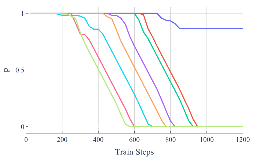
Figure 3: Progressive shrinkage of exemplary mask parameters $\mathbf{p}$ in Attn-V layer $l=30$ of LLaMA-7B based on Equation 8. The starting points of shrinkage are predictive of the pruning order, a typical phenomenon in $\ell_{1}$-regularization. In ACIP, this pruning order determines the score of associated singular values $\mathbf{s}$ (compare Algorithm 1).

Iterative Pruning

The optimization problem solved by ACIP takes the form

$$\min_{\mathbf{p},\boldsymbol{\Delta}}\mathcal{L}\bigl{(}\mathbf{X};\boldsymbol{\theta},\mathbf{p},\boldsymbol{\Delta}\bigr{)}+\lambda\left\lVert\mathbf{p}\right\rVert_{1},$$ (8)

where $\mathcal{L}$ denotes a suitable calibration loss for the model, $\mathbf{p}=\{\mathbf{p}_{0},\dots,\mathbf{p}_{L}\}$ the set of all mask parameters, $\boldsymbol{\Delta}=\{\boldsymbol{\Delta}_{0},\dots,\boldsymbol{\Delta}_{L}\}$ the set of all low-rank adapters, and $\boldsymbol{\theta}$ the set of all remaining model parameters that are frozen during optimization. We perform optimization until a preset stopping compression rate $r_{\text{stop}}$ is reached (see Section D.2 for further discussion). Optionally, we perform post-tuning for a fixed number of steps by freezing the masks and continue optimizing the low-rank adapters.

Remark 2.1 (Scaling of $\lambda$).

If $\lambda$ is chosen too small, the stopping rate $r_{\text{stop}}$ might never be reached. If $\lambda$ is too large, training might become unstable and the score map ambiguous. Therefore, we use a simple linear scheduler that scales $\lambda$ by a fixed factor $>$1 every $j$ optimization steps, so that pruning becomes increasingly aggressive over time.

From Iterative Pruning to Score Map

We use the optimization process of (8) to inform our score map. Based on the discussion of Section 2.1.3, we hypothesize that there is a close relationship between the order in which the parameters $\mathbf{p}_{l}^{(i)}$ are pruned and their importance for the model — the least important parameters are pruned first and so on. During experimentation, we observed a shrinkage behavior that supports this hypothesis (see Figure 3).

Algorithm 1 describes how the score map is updated after each optimization step. In plain words, the score map is built based on the pruning order. A negative number in the map indicates how many steps ago a parameter was pruned. For all parameters that have not been pruned, the score is set to the value of the corresponding parameter. We refer to Section D.7 for visual examples of ACIP score maps.

Algorithm 1 ensures that (i) the score map stores the pruning history, and (ii) it estimates future pruning based on the parameter magnitudes. Note that absolute values of the score are irrelevant for parameter ranking.

Algorithm 1 Score map generation

⬇

# params: parameters p, vectorized;

# scores: pruning scores, vectorized;

# initialized to NaN

def update_scores(scores, params):

# previously pruned parameters

score_mask = scores <= 0.

scores[not score_mask] = params[not score_mask]

scores[score_mask] -= 1.

return scores

2.2.3 Step 3. Any Compression

From the optimization of (8), we obtain two components: (i) the score map that informs model compression and (ii) the tuned low-rank adapters $\boldsymbol{\Delta}$. The pruned masks $\mathbf{m}$ are discarded, as they are irrelevant for compression at this stage (cf. Figure 2). As motivated above, the score map allows us to globally rank all singular vectors based on their score. We can flexibly create a model for any compression rate $r$ by pruning the singular values $\mathbf{s}$ (and corresponding singular vectors) according to their score $\rho_{l}^{(i)}$. Note that there is a monotonic, but non-linear relationship between the number of total pruned singular values $k$ and compression rate $r$ (cf. Section 2.1.2). Given a target rate $r$, we can easily find $k$ via a binary search.

Finally, for layers with determined rank $k\geq\frac{mn}{m+n}$, we avoid excess storage required by the reparametrization by simply recovering $\mathbf{W}$ from its SVD components.

3 Related work

Post-training compression methods for Foundation Models largely fall into three categories: knowledge distillation, quantization and (un-)structured pruning. For a comprehensive survey covering all of these, we refer to (Zhu et al., 2024) and the references therein.

ACIP represents a specific form of structured pruning: factorization-based compression. Conventional structured pruning (Frantar & Alistarh, 2023; Xia et al., 2024; Ashkboos et al., 2024) jointly removes groups of parameters (e.g., network layers or matrix columns/rows). At high compression rates, however, such coarse approaches often remove important weights, causing a significant performance drop that is only recoverable through additional fine-tuning.

Low-Rank Decomposition

Approximation of weight matrices through appropriate factorization aims to preserve critical information while being simple to implement. After initial exploration for smaller language models (Edalati et al., 2022; Tahaei et al., 2022), methods for LLMs primarily built on (weighted) SVD of linear layers (Ben Noach & Goldberg, 2020; Hsu et al., 2022). Large approximation errors, however, made additional fine-tuning on down-stream tasks necessary.

Follow-up work recognized that the poor approximations are caused by LLM weights being high-rank and instead turned to decompose network features which are sparse (Kaushal et al., 2023; Yu & Wu, 2023). Notably, ASVD (Yuan et al., 2024) explicitly accounts for the data distribution eliciting these activations and SVD-LLM (Wang et al., 2024) derives an analytical layer-wise correction.

Recent studies (Sharma et al., 2023; Yuan et al., 2024; Jaiswal et al., 2024) have shown rank reduction to differently affect layers in a network and proposed different heuristics for non-uniform pruning of singular values.

A common feature of these works is that they first truncate singular values to a desired size before computing an error correction. A change in compression ratio therefore prompts another round of computation. At the same time, the correction quality varies across different ratios, so that milder compression may not automatically preserve more predictive quality. In contrast, our approach creates consistent compression trade-offs from a single round of computation (optimization) and performs corrections on-the-fly.

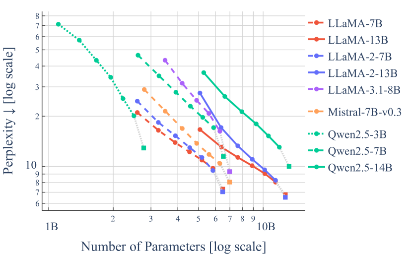
Figure 4: Compression-performance trade-off curves generated by ACIP on C4. Compared to Figure 1, we plot over the actual model parameter sizes to enable cross-model comparison. Square marks denote the base model performance.

Rate-distortion theory

Rate-distortion theory investigates the analytical trade-off between achievable data compression rates and the error (distortion) introduced by general lossy compression algorithms (Cover & Thomas, 2006). While some recent work (Gao et al., 2019; Isik et al., 2022) investigates rate-distortion theory of machine learning models for simple architectures under rather specific assumptions, the information-theoretic limits of neural network compression are generally unknown in practically relevant settings. In this context, the family of compressed models generated by ACIP conveniently provides an empirical (upper) bound on the distortion-rate function of a large-scale model from a single optimization run.

4 Experiments

Experimental Setup

Table 1: Zero-shot evaluation of LLaMA-7B, comparing with existing SVD-based compression methods ASVD (Yuan et al., 2024) and SVD-LLM (Wang et al., 2024). $\uparrow$: larger is better; $\downarrow$: smaller is better; best results for each task and size ratio are marked in bold. The scores for ASVD and SVD-LLM are taken from Wang et al. (2024).

		C4 ↓	WikiText-2 ↓	Openb. ↑	ARC_e ↑	WinoG. ↑	HellaS. ↑	ARC_c ↑	PIQA ↑	MathQA ↑	LM Eval Avg. ↑
Size	Method
100%	Original	7.34	5.68	0.28	0.67	0.67	0.56	0.38	0.78	0.27	0.52
80%	ASVD	15.93	11.14	0.25	0.53	0.64	0.41	0.27	0.68	0.24	0.43
	SVD-LLM	15.84	7.94	0.22	0.58	0.63	0.43	0.29	0.69	0.24	0.44
	ACIP (ours)	10.92	8.83	0.28	0.66	0.63	0.49	0.32	0.74	0.23	0.48
70%	ASVD	41.00	51.00	0.18	0.43	0.53	0.37	0.25	0.65	0.21	0.38
	SVD-LLM	25.11	9.56	0.20	0.48	0.59	0.37	0.26	0.65	0.22	0.40
	ACIP (ours)	12.22	10.35	0.28	0.64	0.62	0.47	0.31	0.73	0.23	0.47
60%	ASVD	1109.00	1407.00	0.13	0.28	0.48	0.26	0.22	0.55	0.19	0.30
	SVD-LLM	49.83	13.11	0.19	0.42	0.58	0.33	0.25	0.60	0.21	0.37
	ACIP (ours)	13.91	12.46	0.25	0.61	0.59	0.44	0.30	0.71	0.24	0.45
50%	ASVD	27925.00	15358.00	0.12	0.26	0.51	0.26	0.22	0.52	0.19	0.30
	SVD-LLM	118.57	23.97	0.16	0.33	0.54	0.29	0.23	0.56	0.21	0.33
	ACIP (ours)	16.47	16.16	0.21	0.57	0.57	0.40	0.27	0.68	0.22	0.42
40%	ASVD	43036.00	57057.00	0.12	0.26	0.49	0.26	0.21	0.51	0.18	0.29
	SVD-LLM	246.89	42.30	0.14	0.28	0.50	0.27	0.22	0.55	0.21	0.31
	ACIP (ours)	21.05	23.99	0.19	0.49	0.55	0.35	0.24	0.64	0.21	0.38

To demonstrate effectiveness across architectural differences in LLMs, we evaluate ACIP on a range of popular open-weight models: LLaMA-7B/13B (Touvron et al., 2023a), LLaMA-2-7B/13B (Touvron et al., 2023b), LLaMA-3.1-8B (Grattafiori et al., 2024), Qwen2.5-7B/14B (Qwen et al., 2024), and Mistral-7B-v0.3 (Jiang et al., 2023). More detailed analyses and ablations are carried out with LLaMA-7B as it was most extensively studied in previous research on structured weight pruning. Regarding evaluation tasks, we follow (Wang et al., 2024) and report perplexity on validation held-outs of C4 (Raffel et al., 2019) and WikiText-2 (Merity et al., 2017), and consider seven zero-shot tasks from EleutherAI LM Evaluation Harness (LM-Eval) (Gao et al., 2023). Implementation details about ACIP and choices of hyperparameters can be found in Appendix B.

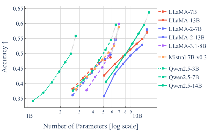
Figure 5: Compression-performance trade-off curves generated by ACIP, using average accuracy on all LM-Eval tasks as metric.

4.1 Analyzing Compression-Performance Trade-Offs

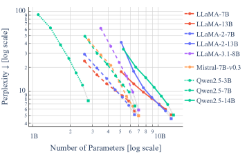
(a) WikiText-2

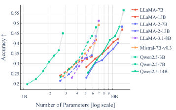
(b) ARC Challenge

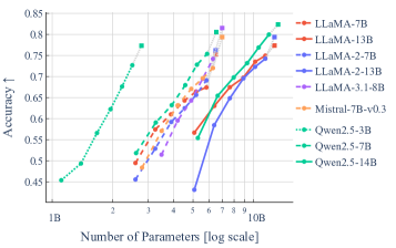
(c) ARC Easy

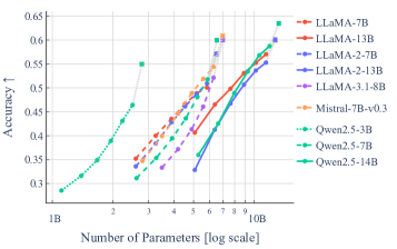
(d) HellaSwag

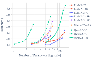
(e) MathQA

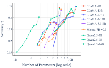
(f) OpenBookQA

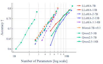
(g) PIQA

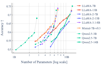
(h) Winogrande

Figure A8: Compression-performance trade-off curves generated by ACIP on WikiText-2 and individual LM-Eval tasks, complementing the results of Figure 4 and Figure 5.

Picking up the introductory discussion of Figure 1, we now study compression-performance trade-offs of ACIP in more detail. Figure 4 and Figure 5 confirm smooth and consistent curve shapes for all considered models; analogous results for Wikitext-2 and individual zero-shot LM-Eval tasks can be found in Figure A8. A remarkable observation is that the oldest models, LLaMA-7B/13B, perform best perplexity-wise, while newer, more capable models like Qwen2.5-7B/14B dominate on LM-Eval as expected, especially on the lower compression levels. This apparent contradiction is likely caused by a deviation of the LLM pre-training data distributions from C4. In fact, more recent models use much larger and more diverse training corpora.

A second noteworthy outcome of Figure 4 and Figure 5 are the gaps between LLMs of different base model sizes in the same family. Indeed, ACIP cannot match the performance of base models of smaller size, e.g., compare the compressed Qwen2.5-7B with the original Qwen2.5-3B. This is not surprising because the corresponding smaller-size base models were obtained by pre-training or knowledge distillation, which are orders of magnitudes more expensive than ACIP.

Comparison to Existing Works

We now compare ACIP to two recent works focusing on SVD-based structured pruning, namely ASVD (Yuan et al., 2024) and SVD-LLM (Wang et al., 2024). Both approaches are backpropagation-free and perform (activation-aware) layer-wise updates instead. Table 1 shows that ACIP consistently outperforms both methods with a growing gap for higher compression levels. Note that SVD-LLM was calibrated on Wikitext-2 instead of C4, which might explain slightly better results on the former dataset for 70% and 80% size. We think that these results underpin the benefits of an end-to-end scheme: (i) a simultaneous correction, e.g., by LoRA, can drastically improve performance, and (ii) robust pruning patterns can be found without leveraging any specific features of the SVD factorization. Moreover, note that recomputations are required to generate each row of Table 1 for ASVD and SVD-LLM, whereas ACIP only needs a single run. Analogous results for ACIP applied to all other models can be found in Table A2.

4.2 Improving Performance Through Fine-Tuning

While the main goal of this work is to produce a full family of accurate, compressed models from a few optimization steps, their performance can be certainly improved through continued fine-tuning. Figure 6 highlights the gains of fine-tuning LLaMA-7B; see Table A2 for more detailed numerical results on all other models. We observe that fine-tuning leads to a performance offset that is almost constant across all compression levels, which underlines the predictive capacity of ACIP. Note that we even observe a jump at zero compression because inserting the low-rank adapter learned by ACIP leads to a slight initial performance drop.

We argue that post-compression fine-tuning should be still seen as an independent (and much more costly) algorithmic step for two reasons. (i) Its outcome strongly depends on the specific training protocol and data, making a fair comparison challenging (cf. Q3 in Appendix A); (ii) it requires us to fix a compression level, which breaks the crucial any-compression-feature of ACIP.

4.3 Combining ACIP with Quantization

In the field of low-cost compression for LLMs, quantization is still considered as the gold standard (Hohman et al., 2024; Zhu et al., 2024), so that a practitioner might not be willing to exchange its gains for the benefits of ACIP. Fortunately, ACIP only tunes a tiny fraction of weights with high precision, so that all remaining modules are suitable for quantization. In our experiments, we quantize all parameterized and unparametrized linear layers to $4$-bit in fp4-format (Dettmers et al., 2023) using the bitsandbytes-Package (W4A16), except for the embedding layer and final classification head. We study the gains of quantization for ACIP in the following two ways.

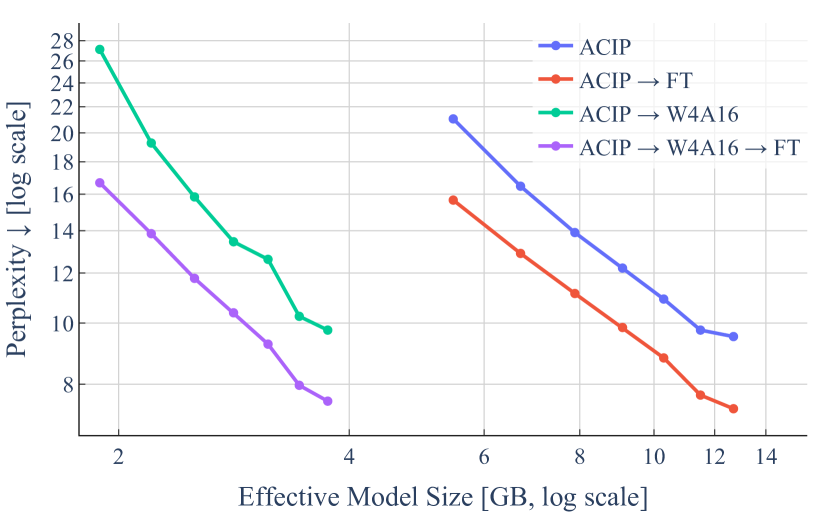
Figure 6: Compression-performance trade-off curves for LLaMA-7B on C4 showing the impact of fine-tuning and quantization after compression with ACIP. The horizontal axis measures size in terms of required (weight) memory to visualize the gains of quantization more clearly.

Compress first, then quantize.

We first apply ACIP as usual, compress the model to a given target size, and then quantize all remaining linear layers. Figure 6 confirms that this approach works fairly well, only producing a slight performance drop compared to non-quantized versions; see Table A3 for a full evaluation on all other metrics. We also observe that an optional fine-tuning step as in Section 4.2 can almost fully compensate for the errors introduced by quantization after compression. This finding is well in line with the effectiveness of the popular QLoRA approach (Dettmers et al., 2023). Moreover, Figure 6 reveals a drastic improvement through quantization in terms of required memory. Here, the ACIP-trade-off allows practitioners to study and apply a more fine-grained compression on top of quantization.

Quantize first, then compress and transfer.

Compared to layer-wise methods like ASVD and SVD-LLM, ACIP has a higher demand in GPU memory due to backpropagation. A quantization of all frozen weight matrices can be an effective remedy in this respect. For the experiment shown in Figure 7, we have applied quantization before ACIP, which leads to very similar compression-performance trade-offs as in the non-quantized case. Going one step further, we transfer the score maps and low-rank adapters from this quantized version of ACIP back to full precision: We load the base model in bf16, apply layer-wise SVD-parametrization, insert the low-rank adapters learned by quantized ACIP, and use the corresponding score map to obtain a compressed model (W16A16). The resulting trade-off curve in Figure 7 confirms that this simple strategy works fairly well, especially for lower compression levels.

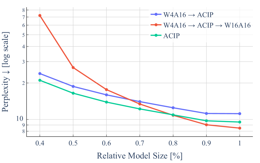
Figure 7: Compression-performance trade-off curves for LLaMA-7B on C4, showing that quantization before ACIP leads to similar results as without.

Further Experiments and Ablations

Several additional experiments are presented in Appendix D, analyzing the impact of several key components and design aspects of ACIP.

5 Conclusion

In this work, we have introduced Any Compression via Iterative Pruning (ACIP), a simple end-to-end algorithm to determine the compression-performance trade-off of large pre-trained models. The underlying score map ranking allows us to materialize models of any compression rate from a single optimization run. We have demonstrated empirically that the downstream performance of the resulting models is superior to existing, layer-wise factorization approaches. The flexibility and efficiency of ACIP make it a practical tool for deploying large-scale models in resource-constrained settings, especially in combination with other compression techniques such as quantization.

Limitations and Outlook

Our main results in Figure 4 and Figure 5 resemble the well-known phenomenon of scaling laws (Kaplan et al., 2020; Hoffmann et al., 2022). We believe that this association is not a coincidence. But revealing a more rigorous connection goes beyond the scope of this work. In a similar vein, we observe that more recent models tend to be less compressible (e.g., compare the slopes of LLaMA-13B and Qwen2.5-14B in Figure 5). We hypothesize that this relates to the fact that newer models carry more dense information per weight, since they were trained on much larger datasets (Allen-Zhu & Li, 2024). Also, the distribution of the calibration dataset (C4 in our case) might play an important role in this context.

A notable limitation of our work is that we have only focused on models that are tunable on a single (NVIDIA H100) GPU in bf16-precision. Hence, the scaling behavior of ACIP for larger LLMs (30B+) remains to be explored. Finally, we emphasize that ACIP could be transferred to other modalities, architectures, and tasks without any notable modifications.

Software and Data

Code will be made available on Github soon.

Appendix A Question & Answers

In this section, we discuss a few common questions about our method and experimental design that were not (fully) addressed in the main part due to length restrictions.

• Why did you not directly compare your results to quantization and full-weight (unstructured) pruning?

• We argue that these are fundamentally different compression approaches. Full weight manipulations, in principle, have the potential to lead to more powerful compressions because they have more degrees of freedom (analogously to full-weight fine-tuning vs. PEFT). Therefore, they should not be seen as competing methods but complementary ones. We admit that practitioners probably would not favor ACIP over well-established and widely supported quantization techniques. However, the adapter-style nature of ACIP makes it suitable for a combination which can lead to extra gains, as demonstrated in Section 4.3.

• Why did you not compare with model distillation or combined ACIP with it?

• While model distillation can lead to outstanding compression results, e.g., see (Raschka, 2024), this approach requires significantly more resources than ACIP, typically orders of magnitudes more. A direct comparison is therefore not meaningful from our point of view, as it should at least be based on approximately the same computational budget.

• Why did you not compare your fine-tuning results with other factorization-based methods?

• Some previous works on SVD-based pruning (Wang et al., 2024; Jaiswal et al., 2024) report results on post-compression fine-tuning as well. While our own results in Table A2 are highly competitive in this respect, we decided to omit a direct comparison because: (i) the downstream performance strongly depends on the exact fine-tuning protocol (datasets, compute budget, hyperparameters, etc.) which we were not able to fully recover from published code; and (ii) as pointed out in Section 4.2, promoting a costly fine-tuning step after compression is not the primary concern of our work.

• Why do you propose a backpropagation-based algorithm instead of layer-wise weight updates?

• Let us first summarize several benefits of our end-to-end optimization approach from the main paper: (i) it is conceptually simple and requires no feature engineering, (ii) an error correction can be injected with almost no extra costs, (iii) it allows us to perform efficient and accurate any-size compression.

  Apart from that, and to the best of our knowledge, existing compression algorithms that use layer-wise updates like ASVD (Yuan et al., 2024), SVD-LLM (Wang et al., 2024), or WeLore (Jaiswal et al., 2024) require a separate fine-tuning step to achieve competitive downstream performance. Therefore, the lower costs of layer-wise compression are actually dominated by a more expensive backpropagation-based step. It remains open if similar results can be obtained by a fully tuning-free algorithm.

• Why do you use matrix factorization, and SVD in particular?

• Committing to a backpropagation-based algorithm (see Q4) means that we have to deal with increased memory requirements. As such, matrix factorization is not helpful in that respect because the number of parameters might even increase initially (for instance, an SVD-parametrization basically doubles the size of a quadratic weight matrix). On the other hand, tuning and pruning only the bottleneck layer (i.e., the singular value mask in case of ACIP) has the potential for drastic size reductions and is highly parameter-efficient. For example, the number of tunable mask parameters for LLaMA-7B with ACIP is $<$1M.

  With this in mind, SVD as a specific matrix factorization is an obvious candidate due to its nice mathematical and numerical properties, in particular, optimal low-rank matrix approximation and stable matrix operations due to orthogonality.

Appendix B Implementation Details

In this section, we report more technical details and hyperparameters used for our experiments.

Dataset and Models

Following previous work on LLM compression, we use C4 for training as it is a good proxy of a general-purpose dataset. In the context of ACIP, it should be primarily seen as a calibration dataset that allows us to propagate meaningful activations through a pre-trained model while performing structured pruning. Overfitting to the distribution of C4 is implicitly mitigated, since we only tune very few parameters (masks and LoRA-adapters) compared to the total model size.

All considered (evaluation) datasets and pre-trained models are imported with the HuggingFace transformers-library in bfloat16-precision. Our experiments were implemented with PyTorch (Paszke et al., 2019) and the Lightning package.

ACIP-Specifics

As mentioned in Remark 2.1, we apply a linear scheduler that increases the regularization parameter $\lambda$ dynamically over the pruning process. This ensures that the pruning becomes more and more aggressive over time and the stopping criterion will be reached at some point. Across all experiments, we use $\lambda=1e{-}3$ as initial value and increase it by a factor of $1.01$ every $4$ steps (this amounts to a doubling $\lambda$ at about every $280$ steps).

As pointed out in Section 2.2.2, we choose a (maximum) target compression rate as a stopping criterion for ACIP. In most experiments, a rate of $r_{\text{stop}}=0.4$ is reasonable (i.e., only 40% or the original parameters remain), and we refer to Section D.2 for further discussion and analysis. After the stopping criterion is reached with tune the low-rank adapter for 1K more steps while the masks are frozen (see Section 2.2.2).

The mask parameters in (7) are rescaled by a fixed factor of $0.02$ to ensure a better alignment with the numerical range of the remaining network weights. The low-rank adapters are created with $r=32$, $\alpha=16$, and dropout $0.05$. For LLaMA-7B, the number of tunable parameters amounts to $<$1M mask parameters and approximately 80M low-rank adapter parameters.

For sample data from C4, we use $1024$ tokens per sample and a batch size of $4$. We use Adam (Kingma & Ba, 2015) as optimizer without weight decay and a learning rate of $5e{-}5$.

Runtime Analysis

ACIP requires significantly fewer steps than fine-tuning. Depending on when the stopping criterion is reached, it typically takes 1.5K - 2.5K steps, including 1K post-tuning steps of the low-rank adapters. For LLaMA-7B, for example, this amounts to a wall clock runtime of $<30$ minutes, including the initial SVD computations for the base model parametrization. All runs were performed on single NVIDIA H100 GPUs.

Fine-Tuning

In all post-compression fine-tunings (see Section 4.2), we simply continue training ACIP’s low-rank adapters (the optimizer states are reset). We train for $20$K-$25$K steps on C4 with a batch size of $4$ and a learning rate of $2e{-}4$.

Appendix C Supplementary Results for Section 4.1 – Section 4.3

Figure A8 complements the trade-off curves in Figure 4 and Figure 5 by all other considered evaluation metrics (see Section 4.1). Table A2 reports these results in terms of numbers, including all fine-tuning results for all models (see Section 4.2). Table A3 provides more detailed evaluation results on fine-tuning a quantized and compressed LLaMA-7B model (see Section 4.3).

Table A2: Evaluation results for ACIP on all considered LLMs. Scores on C4 and WikiText-2 are measured in perplexity (smaller is better), and the LM-Eval zero-shot tasks are measured in accuracy (higher is better). ^∗The results of LLaMA2-13B were achieved by ignoring all up-projection layers in ACIP (see Section D.6 for more details).

		C4 ↓		WikiText-2 ↓		ARC_c ↑		ARC_e ↑		HellaS. ↑		MathQA ↑		Openb. ↑		PIQA ↑		WinoG. ↑		LM Eval Avg. ↑
	Type	ACIP	FT	ACIP	FT	ACIP	FT	ACIP	FT	ACIP	FT	ACIP	FT	ACIP	FT	ACIP	FT	ACIP	FT	ACIP	FT
Model	Size
LLaMA-7B	40%	21.05	15.66	23.99	17.33	0.24	0.24	0.49	0.53	0.35	0.38	0.21	0.21	0.19	0.20	0.64	0.67	0.55	0.57	0.38	0.40
	50%	16.47	12.89	16.16	11.88	0.27	0.27	0.57	0.59	0.40	0.43	0.22	0.23	0.21	0.23	0.68	0.71	0.57	0.60	0.42	0.44
	60%	13.91	11.14	12.46	9.63	0.30	0.32	0.61	0.64	0.44	0.47	0.24	0.23	0.25	0.26	0.71	0.73	0.59	0.63	0.45	0.47
	70%	12.22	9.84	10.35	8.27	0.31	0.34	0.64	0.69	0.47	0.50	0.23	0.24	0.28	0.28	0.73	0.75	0.62	0.66	0.47	0.49
	80%	10.92	8.81	8.83	7.19	0.32	0.38	0.66	0.71	0.49	0.53	0.23	0.24	0.28	0.31	0.74	0.77	0.63	0.68	0.48	0.52
	90%	9.75	7.69	7.56	6.12	0.33	0.39	0.67	0.73	0.50	0.56	0.25	0.25	0.27	0.33	0.76	0.78	0.63	0.69	0.49	0.53
	100%	9.52	7.32	7.20	5.75	0.33	0.40	0.69	0.75	0.51	0.57	0.25	0.26	0.26	0.34	0.76	0.79	0.63	0.70	0.49	0.54
	Original	7.31		5.68		0.42		0.75		0.57		0.27		0.34		0.79		0.70		0.55
LLaMA-13B	40%	16.64	13.38	17.66	13.42	0.28	0.28	0.57	0.59	0.41	0.43	0.22	0.23	0.23	0.24	0.69	0.70	0.60	0.62	0.43	0.44
	50%	13.06	11.12	12.42	10.49	0.32	0.34	0.63	0.63	0.47	0.48	0.23	0.23	0.26	0.28	0.72	0.73	0.62	0.64	0.47	0.47
	60%	11.33	9.76	9.79	8.30	0.35	0.33	0.67	0.68	0.50	0.51	0.24	0.24	0.28	0.30	0.74	0.76	0.65	0.67	0.49	0.50
	70%	10.10	8.72	8.17	7.06	0.38	0.38	0.70	0.69	0.53	0.54	0.24	0.26	0.31	0.31	0.76	0.77	0.67	0.70	0.51	0.52
	80%	9.06	7.91	6.91	6.21	0.41	0.41	0.74	0.74	0.55	0.57	0.26	0.27	0.32	0.34	0.77	0.78	0.68	0.69	0.53	0.54
	90%	8.04	7.06	5.98	5.40	0.42	0.44	0.75	0.76	0.57	0.59	0.29	0.29	0.32	0.33	0.79	0.79	0.70	0.72	0.55	0.56
	100%	7.86	6.79	5.83	5.15	0.42	0.46	0.75	0.77	0.57	0.60	0.29	0.30	0.31	0.32	0.79	0.79	0.70	0.73	0.55	0.57
	Original	6.77		5.09		0.47		0.77		0.60		0.30		0.33		0.79		0.73		0.57
LLaMA-2-7B	40%	24.62	16.74	29.20	18.00	0.21	0.22	0.46	0.50	0.34	0.37	0.20	0.21	0.18	0.19	0.62	0.66	0.51	0.55	0.36	0.39
	50%	18.36	13.32	19.64	12.25	0.25	0.27	0.53	0.57	0.38	0.42	0.22	0.22	0.24	0.23	0.67	0.69	0.53	0.56	0.40	0.42
	60%	15.27	11.15	14.47	9.54	0.28	0.31	0.59	0.63	0.43	0.46	0.23	0.24	0.25	0.23	0.69	0.72	0.57	0.62	0.44	0.46
	70%	12.96	9.73	10.47	7.74	0.33	0.35	0.62	0.68	0.46	0.50	0.25	0.24	0.27	0.26	0.73	0.74	0.60	0.64	0.47	0.49
	80%	11.31	8.63	8.46	6.54	0.33	0.37	0.66	0.70	0.49	0.53	0.25	0.26	0.28	0.31	0.74	0.77	0.63	0.66	0.48	0.51
	90%	9.46	7.43	6.69	5.45	0.34	0.43	0.69	0.75	0.51	0.56	0.26	0.28	0.28	0.33	0.76	0.78	0.63	0.69	0.50	0.54
	100%	9.34	7.06	6.54	5.13	0.34	0.43	0.70	0.76	0.51	0.57	0.26	0.28	0.27	0.32	0.76	0.78	0.64	0.69	0.50	0.55
	Original	7.04		5.11		0.44		0.76		0.57		0.28		0.31		0.78		0.69		0.55
LLaMA-2-13B	40%	27.55	84.28	41.22	145.79	0.23	0.23	0.43	0.46	0.33	0.30	0.21	0.21	0.18	0.18	0.62	0.63	0.52	0.52	0.36	0.36
	50%	17.10	12.76	17.89	13.12	0.30	0.32	0.58	0.61	0.41	0.44	0.21	0.23	0.27	0.27	0.69	0.70	0.56	0.58	0.43	0.45
	60%	13.29	10.05	11.11	8.43	0.32	0.36	0.65	0.68	0.47	0.50	0.22	0.23	0.29	0.31	0.72	0.74	0.60	0.63	0.47	0.49
	70%	11.04	8.64	8.40	6.71	0.35	0.41	0.70	0.74	0.51	0.54	0.23	0.25	0.30	0.33	0.74	0.77	0.62	0.66	0.49	0.53
	80%	9.54	7.68	6.80	5.66	0.37	0.44	0.72	0.76	0.54	0.57	0.25	0.28	0.30	0.34	0.77	0.78	0.64	0.71	0.51	0.55
	90%	8.26	6.86	5.70	4.87	0.40	0.47	0.74	0.78	0.55	0.60	0.26	0.31	0.31	0.34	0.78	0.79	0.66	0.72	0.53	0.57
	100%	7.87	6.56	5.42	4.61	0.41	0.47	0.75	0.79	0.56	0.60	0.28	0.32	0.31	0.35	0.78	0.79	0.69	0.71	0.54	0.58
	Original	6.52		4.57		0.48		0.79		0.60		0.32		0.35		0.79		0.72		0.58
LLaMA-3.1-8B	50%	43.32	26.52	61.77	29.52	0.23	0.27	0.51	0.58	0.33	0.37	0.22	0.23	0.17	0.19	0.64	0.68	0.53	0.54	0.38	0.41
	60%	31.55	21.00	36.69	19.26	0.29	0.29	0.60	0.61	0.37	0.42	0.24	0.24	0.22	0.23	0.69	0.72	0.55	0.56	0.42	0.44
	70%	24.90	17.08	23.06	13.55	0.33	0.32	0.64	0.66	0.41	0.47	0.26	0.27	0.23	0.27	0.71	0.73	0.59	0.62	0.45	0.48
	80%	20.78	14.21	15.60	10.12	0.38	0.40	0.69	0.72	0.46	0.51	0.28	0.30	0.28	0.29	0.74	0.77	0.61	0.66	0.49	0.52
	90%	16.25	11.28	9.80	7.24	0.41	0.48	0.74	0.80	0.52	0.57	0.33	0.35	0.27	0.31	0.77	0.79	0.67	0.71	0.53	0.57
	100%	14.57	9.42	8.04	5.95	0.40	0.51	0.75	0.82	0.53	0.60	0.36	0.40	0.27	0.34	0.78	0.80	0.66	0.74	0.54	0.60
	Original	9.31		5.86		0.51		0.82		0.60		0.39		0.33		0.80		0.74		0.60
Mistral-7B-v0.3	40%	28.92	19.21	44.29	23.24	0.24	0.26	0.48	0.53	0.35	0.38	0.21	0.21	0.18	0.19	0.66	0.67	0.55	0.57	0.38	0.40
	50%	21.44	14.86	28.60	16.53	0.28	0.28	0.57	0.59	0.40	0.43	0.21	0.23	0.22	0.21	0.69	0.70	0.58	0.60	0.42	0.43
	60%	16.89	12.49	21.19	12.29	0.32	0.32	0.63	0.66	0.45	0.48	0.24	0.24	0.20	0.23	0.72	0.73	0.60	0.62	0.45	0.47
	70%	13.75	10.95	13.28	9.69	0.35	0.34	0.67	0.68	0.49	0.52	0.27	0.28	0.21	0.26	0.74	0.76	0.63	0.63	0.48	0.49
	80%	11.80	9.84	8.70	7.49	0.38	0.39	0.70	0.73	0.52	0.55	0.29	0.29	0.23	0.26	0.76	0.77	0.65	0.69	0.50	0.53
	90%	10.42	8.84	6.51	5.85	0.40	0.43	0.72	0.75	0.54	0.59	0.31	0.33	0.25	0.31	0.78	0.79	0.68	0.70	0.53	0.56
	100%	9.85	8.31	6.04	5.31	0.40	0.45	0.73	0.77	0.55	0.60	0.33	0.34	0.26	0.33	0.78	0.79	0.68	0.72	0.53	0.57
	Original	8.05		4.96		0.49		0.79		0.61		0.36		0.34		0.80		0.73		0.59
Qwen2.5-3B	40%	71.23	36.85	91.51	39.44	0.20	0.22	0.45	0.51	0.29	0.31	0.21	0.22	0.15	0.16	0.60	0.64	0.50	0.52	0.34	0.37
	50%	57.17	29.43	62.42	26.92	0.22	0.25	0.49	0.57	0.32	0.34	0.22	0.21	0.18	0.19	0.63	0.67	0.52	0.53	0.37	0.39
	60%	43.30	23.30	38.26	18.38	0.26	0.29	0.57	0.63	0.35	0.39	0.23	0.23	0.21	0.24	0.67	0.69	0.54	0.56	0.40	0.43
	70%	34.24	19.04	25.81	13.50	0.31	0.34	0.62	0.68	0.39	0.43	0.25	0.26	0.24	0.26	0.70	0.72	0.57	0.58	0.44	0.47
	80%	25.50	16.16	17.02	10.68	0.34	0.36	0.68	0.73	0.43	0.47	0.28	0.31	0.26	0.24	0.72	0.74	0.58	0.57	0.47	0.49
	90%	20.10	13.82	11.99	8.57	0.37	0.42	0.73	0.77	0.46	0.52	0.33	0.36	0.27	0.33	0.74	0.78	0.60	0.67	0.50	0.55
	100%	18.73	12.81	10.63	7.70	0.36	0.47	0.72	0.78	0.46	0.54	0.33	0.41	0.24	0.31	0.74	0.78	0.60	0.69	0.49	0.57
	Original	12.90		7.64		0.45		0.77		0.55		0.37		0.30		0.78		0.68		0.56
Qwen2.5-7B	40%	46.43	29.26	49.04	27.24	0.23	0.24	0.52	0.58	0.31	0.34	0.22	0.21	0.19	0.20	0.64	0.67	0.53	0.53	0.38	0.40
	50%	34.90	23.26	29.96	19.72	0.27	0.30	0.59	0.64	0.35	0.39	0.22	0.23	0.23	0.25	0.67	0.70	0.54	0.57	0.41	0.44
	60%	27.84	18.73	21.98	13.73	0.31	0.33	0.63	0.68	0.39	0.45	0.25	0.26	0.25	0.28	0.70	0.73	0.55	0.60	0.44	0.48
	70%	22.97	15.96	15.72	10.71	0.35	0.42	0.68	0.74	0.44	0.49	0.28	0.30	0.29	0.30	0.73	0.76	0.57	0.63	0.48	0.52
	80%	19.68	14.02	12.07	8.89	0.40	0.46	0.73	0.78	0.48	0.53	0.33	0.36	0.30	0.33	0.75	0.78	0.59	0.67	0.51	0.56
	90%	17.09	12.59	9.82	7.63	0.44	0.48	0.75	0.80	0.52	0.56	0.39	0.41	0.31	0.32	0.77	0.79	0.64	0.70	0.54	0.58
	100%	15.34	11.43	8.38	6.60	0.43	0.50	0.75	0.82	0.53	0.59	0.43	0.46	0.28	0.34	0.77	0.79	0.66	0.72	0.55	0.60
	Original	11.47		6.55		0.48		0.81		0.60		0.43		0.34		0.79		0.73		0.60
Qwen2.5-14B	40%	36.51	25.58	33.78	22.22	0.26	0.29	0.55	0.61	0.36	0.38	0.22	0.23	0.24	0.26	0.67	0.68	0.54	0.57	0.41	0.43
	50%	26.27	19.53	20.15	14.57	0.32	0.33	0.65	0.68	0.43	0.44	0.25	0.25	0.26	0.27	0.70	0.71	0.57	0.59	0.45	0.47
	60%	21.29	15.63	14.87	10.48	0.36	0.40	0.70	0.73	0.49	0.51	0.28	0.32	0.28	0.31	0.74	0.76	0.62	0.66	0.50	0.53
	70%	17.99	13.99	11.25	8.89	0.42	0.43	0.73	0.76	0.53	0.54	0.33	0.36	0.31	0.32	0.77	0.78	0.64	0.68	0.53	0.55
	80%	15.23	11.97	8.73	7.11	0.44	0.48	0.77	0.78	0.57	0.58	0.39	0.44	0.34	0.36	0.78	0.79	0.68	0.73	0.57	0.60
	90%	13.05	10.77	6.86	6.04	0.48	0.52	0.80	0.82	0.59	0.60	0.49	0.49	0.32	0.35	0.79	0.81	0.70	0.74	0.60	0.62
	100%	12.37	9.98	6.23	5.11	0.47	0.53	0.79	0.82	0.58	0.62	0.51	0.53	0.32	0.35	0.79	0.81	0.73	0.77	0.60	0.63
	Original	9.99		5.05		0.56		0.82		0.63		0.53		0.35		0.81		0.75		0.64

Table A3: More detailed evaluation results for our quantization experiments from Section 4.3, reported in terms of numbers.

		Eff. model size [GB]	C4 ↓	WikiText-2 ↓	ARC_c ↑	ARC_e ↑	HellaS. ↑	MathQA ↑	Openb. ↑	PIQA ↑	WinoG. ↑	LM Eval Avg. ↑
Size	Ablation
40%	ACIP	5.47	21.05	24.00	0.24	0.49	0.35	0.21	0.19	0.65	0.55	0.38
	ACIP → FT	5.47	15.66	17.33	0.24	0.53	0.38	0.21	0.20	0.67	0.57	0.40
	ACIP → W4A16	1.89	27.12	35.40	0.22	0.46	0.33	0.20	0.18	0.62	0.53	0.36
	ACIP → W4A16 → FT	1.89	16.67	18.90	0.23	0.52	0.37	0.22	0.20	0.67	0.57	0.40
50%	ACIP	6.70	16.47	16.17	0.28	0.58	0.40	0.22	0.21	0.68	0.57	0.42
	ACIP → FT	6.70	12.89	11.88	0.27	0.59	0.43	0.23	0.23	0.71	0.60	0.44
	ACIP → W4A16	2.21	19.28	19.96	0.26	0.54	0.37	0.21	0.20	0.67	0.55	0.40
	ACIP → W4A16 → FT	2.21	13.85	13.33	0.25	0.58	0.41	0.23	0.23	0.70	0.59	0.43
60%	ACIP	7.88	13.91	12.46	0.30	0.61	0.43	0.23	0.25	0.71	0.60	0.45
	ACIP → FT	7.88	11.14	9.63	0.32	0.64	0.47	0.23	0.26	0.73	0.63	0.47
	ACIP → W4A16	2.51	15.84	14.64	0.29	0.58	0.42	0.22	0.22	0.69	0.57	0.43
	ACIP → W4A16 → FT	2.51	11.77	10.31	0.29	0.64	0.45	0.22	0.26	0.72	0.61	0.46
70%	ACIP	9.10	12.22	10.34	0.31	0.64	0.47	0.23	0.27	0.73	0.62	0.47
	ACIP → FT	9.10	9.84	8.27	0.34	0.69	0.50	0.24	0.28	0.75	0.66	0.49
	ACIP → W4A16	2.83	13.45	11.80	0.29	0.63	0.45	0.23	0.24	0.72	0.60	0.45
	ACIP → W4A16 → FT	2.83	10.38	8.74	0.32	0.67	0.48	0.23	0.28	0.75	0.64	0.48
80%	ACIP	10.30	10.91	8.83	0.33	0.67	0.49	0.23	0.28	0.74	0.63	0.48
	ACIP → FT	10.30	8.81	7.19	0.38	0.71	0.53	0.24	0.31	0.77	0.68	0.52
	ACIP → W4A16	3.13	12.61	9.87	0.32	0.65	0.47	0.23	0.28	0.74	0.61	0.47
	ACIP → W4A16 → FT	3.13	9.26	7.60	0.36	0.69	0.52	0.24	0.30	0.76	0.66	0.50
90%	ACIP	11.50	9.75	7.56	0.34	0.68	0.50	0.25	0.27	0.75	0.63	0.49
	ACIP → FT	11.50	7.69	6.12	0.39	0.73	0.56	0.25	0.33	0.78	0.69	0.53
	ACIP → W4A16	3.44	10.25	7.90	0.32	0.66	0.50	0.24	0.27	0.75	0.63	0.48
	ACIP → W4A16 → FT	3.44	7.97	6.39	0.38	0.73	0.56	0.25	0.35	0.78	0.69	0.53
100%	ACIP	12.70	9.52	7.20	0.33	0.69	0.51	0.25	0.26	0.76	0.63	0.49
	ACIP → FT	12.70	7.32	5.75	0.40	0.75	0.57	0.26	0.34	0.79	0.70	0.54
	ACIP → W4A16	3.75	9.75	7.37	0.34	0.69	0.51	0.25	0.27	0.76	0.63	0.49
	ACIP → W4A16 → FT	3.75	7.52	5.94	0.40	0.75	0.56	0.27	0.34	0.78	0.69	0.54

Appendix D Further Experiments and Ablations

In this section, we present several supplementary experiments analyzing the impact of some key algorithmic components and design choices of ACIP in more detail.

D.1 Impact of Low-Rank Adapters

The primary purpose of the low-rank adapters used in ACIP is to correct compression errors on-the-fly during the optimization. A surprising finding of our work is that the final adapters are “universal” in the sense that they can be used across all seen compression levels. While we expect that other PEFT-style approaches would lead to similar findings, it is natural to ask how ACIP would perform without any correction, i.e., just the mask parameters are tuned according to (8). This ablation study is shown in Figure A9. While performing significantly worse than with LoRA, we observe that the perplexity does not blow up and the results are even slightly better than SVD-LLM (see Table 1). This stable behavior of ACIP is closely related to our parameterization of the mask in (7) which ensures that the forward pass corresponds to the actual outputs of the pruned model with binary masks. On the other hand, the straight-through estimator still enables backpropagation.

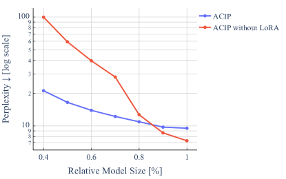
Figure A9: Compression-performance trade-off curves for LLaMA-7B on C4 with and without using a LoRA-adapter for correction in ACIP.

D.2 Impact of the Stopping Criterion

In most experiments, we have used a compression ratio $r_{\text{stop}}$ of $0.4$ as stopping criterion, i.e., the pruning of masks is stopped if the size of the model is only 40% of the original one (measured in number of parameters of all target weight matrices). We have observed that at this point, the model performance has typically dropped so much that even a fine-tuned model would be of limited practical use.

Nevertheless, it is interesting to explore the sensitivity of compression-performance curves against different stopping ratios. The comparison shown in Figure A10 provides several insights in this respect: (i) “Forecasting” compressed models beyond the stopping ratio does not work very well, especially when stopping very early ($>0.8$). (ii) The predictive capacity of ACIP remains valid for even stronger stopping compression ratios than $0.4$. However, finding the largest reasonable stopping ratio is highly model-dependent. For less compressible models like LLaMA-3.1-8B, it could make sense to stop even earlier than $0.4$ (cf. Figure 1). In general, we hypothesize that older models are more compressible than new ones, as the latter “carry” more information per weight due to significantly more training data (Allen-Zhu & Li, 2024).

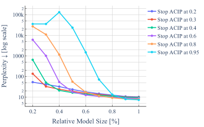
Figure A10: Compression-performance trade-off curves for LLaMA-7B on C4, using different stopping compression ratios  $r_{\text{stop}}$ for ACIP.

D.3 Impact of the Score Map – Forecasting Pruning Patterns

Here, we pick up the observation from Section D.2 that forecasting the performance of compressed models beyond the stop ratio leads to inaccurate predictions, i.e., the model is compressed more strongly than it has been done by ACIP itself. However, it turns out that the score map itself exhibits a certain forecasting capability. To this end, we run ACIP as usual until a stop ratio is reached, say $r_{\text{stop}}=0.4$, but we stop updating the score map earlier in the optimization process. A few compression-performance curves with this modification are reported in Figure A11. We observe very similar curve shapes even if the score map is frozen after only a tiny fraction of mask parameters was pruned. This underpins our intuition from Section 2.2.2 that the pruning path of each parameter is fully determined at very early stage of ACIP.

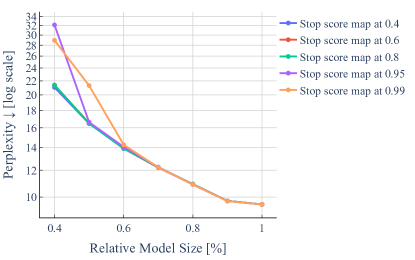
Figure A11: Compression-performance trade-off curves for LLaMA-7B on C4, stopping updates of the score map before the actual stopping criterion of ACIP.

D.4 Impact of the Score Map – A Trivial One Does Not Work

There are certainly alternative ways to design useful score maps. For example, simply accumulating the gradients of all mask parameters entrywise over an ACIP-run works equally well as the strategy proposed in Section 2. It is therefore valid to ask whether one could even design score maps without any optimization. We demonstrate that perhaps the most obvious approach, namely setting the score map equal to the singular values of the weight matrices, does not work very well. Figure A12 shows that this training-free approach does not produce any reasonable compressed models and decent performance cannot be easily recovered with LoRA-finetuning. This simple experiment confirms that designing useful score maps is not a trivial endeavour and requires a carefully crafted algorithmic approach.

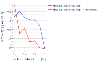
Figure A12: Compression-performance trade-off curves for LLaMA-7B on C4, using a trivial score map based on the initial singular values of the base model.

D.5 Impact of Post-Tuning

Our main experiments are performed with 1K post-tuning steps in ACIP (see the description in Section 2.2.2). Figure A13 shows analogous compression-performance trade-off curves for fewer or no post-tuning steps. We observe that post-tuning can indeed notably increase performance for higher compression ratios.

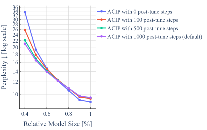
Figure A13: Compression-performance trade-off curves for LLaMA-7B on C4 with different numbers of post-tuning steps in ACIP.

D.6 Impact of Individual Layers – Example of LLaMA2-13B

As pointed out in the caption of Table A2, the linear layers targeted by ACIP were slightly modified for LLaMA2-13, namely all up projection layers were ignored. Figure A14 shows what would happen if they are compressed as well. While the performance predictions for $\geq 0.6$ look decent, the perplexity explodes for stronger compression; note that even additional fine-tuning does not recover a reasonable performance in this situation. We hypothesize that ACIP has pruned one or more singular values of the up projection layers that are crucial for model’s integrity. This finding might be related to the recent work by Yu et al. (2024) on pruning so-called super weights. In any case, ACIP is capable of revealing this undesirable behavior as demonstrated in Figure A14.

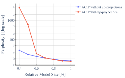
Figure A14: Compression-performance trade-off curves for LLaMA2-13B on C4, (not) ignoring the up projection layers in ACIP.

D.7 Examples of Score Maps Generated by ACIP

Figure A15 and Figure A16 show two typical score maps generated by ACIP for LLaMA-7B and Qwen2.5-7B, respectively. A characteristic feature is that attention layers can be pruned more aggressively than the MLP layers. Similarly, we observe non-uniform pruning patterns for layers of the same type across all transformer layers. This confirms the findings of (Yuan et al., 2024; Jaiswal et al., 2024) and demonstrates that non-uniform structured compression can be achieved without any feature engineering.

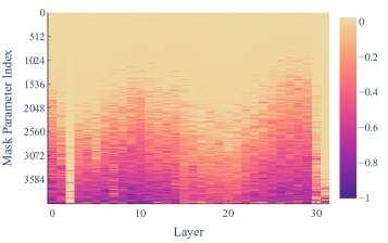
(a) Down Projections

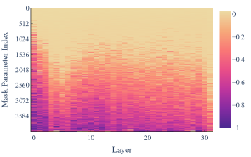
(b) Up Projections

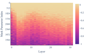
(c) Gate Projections

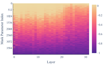
(d) Attention-O

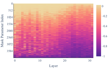
(e) Attention-V

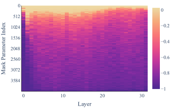
(f) Attention-Q

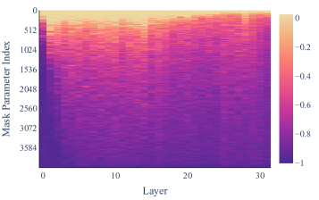
(g) Attention-K

Figure A15: Example score maps generated by ACIP for LLaMA-7B. The negative values (cf. Algorithm 1) are normalized to $-1$ for the purpose of visualization.

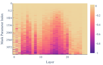
(a) Down Projections

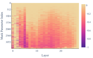
(b) Up Projections

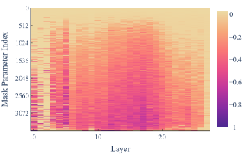
(c) Gate Projections

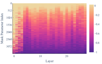
(d) Attention-O

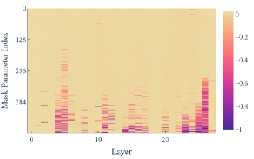
(e) Attention-V

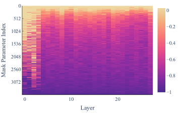
(f) Attention-Q

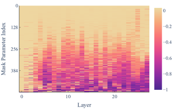
(g) Attention-K

Figure A16: Example score maps generated by ACIP for Qwen2.5-7B. The negative values (cf. Algorithm 1) are normalized to $-1$ for the purpose of visualization.

D.8 Examples of Generated Text by Compressed Models

Table A4 shows examples of generated text by compressed versions of LLaMA-7B.

Table A4: Example texts for two prompts generated for LLaMA-7B under different compressions produced by ACIP.

Size	“How to compress Large Language Models?”	“What is the concept of time?”
Original	I am trying to run a large Language model generation, but I have a few files on disk of around 3gb each. I was wondering if there is a way to compress these files? I have searched the internet but have found nothing. Re: How to compress Large Language Models? I suggest compressing it to HDF5, you can find instructions on how to do this using TensorPacker and PNet on the TensorFlow Github repository …	Have you ever tried to ask a baby what it sees? Time, is it real? What is the concept of time? Have you ever tried to ask a baby what it sees? Let’s see what they can understand. The concept of time. What it is about, who discovered the idea of time, and how was it discovered? How is time measured? We can’t define it. We can’t point at what we are defining, we can’t even show a picture of it …
90%	Jeffrey Hunt, a linguist and applied deep learning researcher at the University of Technology, Sydney, talks with Caleigh Blackstock”s to discuss how to compress a large language model to speed up training and model execution. What does the language model compression actually do to the overall model? …	Please let me know what is the concept of time. The concept of time is all about the measurement of time. This measurement was first done using the hourglass. When this hour Glass was invented, it was the only thing that could represent the passage of time. …
80%	Jeffrey Shafman, Zsolt Nemeth, Jeffrey Shafman, Zsolt Nemeth, Jeffrey Shafman, Zsolt Nemeth. (2013). How to compress Large Language Models? In: ICML proceedings, Vol. 22, pp. 462-463. Magnus Skallman. (2013). How to compress Large Language Models? In: ICML13 Proceedings, pp. 462-463. …	You can’t even imagine that in that time, The life of a tree in nature is as brief As a flash of a lightning bolt, But in this human world, it may endure Through many millennia, if the will of man. So tell me, what is the concept of time? Hey, I’ve got one, and it’s this: …
70%	Apr 04, 2018 at 12:05 pm In the last 5-6 years, Natural Language Systems have been an important direction for my work and the research I do in the course of my PhD. I have been using them to teach myself Swedish and improve my Swedish by machine time in this post. Let’s see if I’ve got it! …	Please tell me where is the concept of time in this poem. What is the significance of the poem ”I Am Wine” by H.W.C. Carson”? What does he mean by the poem title? What does the stairs, the wine, & the man have in common? What does he mean by ”I am wine”? What do you mean by ”I am wine”? …
60%	This is a 14 day free trial. Please use the following link to sign in. Select the country you need here to view pricing and purchase. Whenever you use our web site, we will track your website traffic, the page where you first connected to our site, and the search keywords you use to find us. We’ll use this information to help us continually improve our website. …	You may be wondering what is the concept of time. The concept of time is all about the phenomenon of time. It says that there is never no time. It states that there is always a moment in time. At the moments of time is when we refer the time of life. So, as a matter of the moment, time is just a point in space. …
50%	Jeffrey Huan, Shu-Hua Ji, Xiao-Hong Li, Xiao-Xiao Li, Layin Ma”s. 2019:5, Springer.0000.0001/13/8/19/12/720-22-F43. Miller A. ”The Structure of the Language in Unsupervised Deep-Processing” in Journal of the Acoustical Actors (v. 11(6). 2006:, pp. 278-295). Dong Ming, Sun Jin, He Mei-Chen,’ …	Getting to this answer isn’t that hard. The concept of time is all about the study of time. The study of time isn’t so hard to get a hold on. When you’re younger, you can begin thinking of how much you could have had if you had known how much time you had…if only we had it back then …
40%	Apr 14, 2018 Resumes at The University of Florida will be released on Friday, May 29, 2018 2.05:53pm. Cover your next job announcement with the help of our new Resume Template Builder. To create your own Resume Template in minutes. Improving the quality of your Resume. To improve your Resume …	You may think that it is just a fancy word, or just the idea it had in the earlier world. But there exists a way to understand it. To understand the idea of time by using the example of a clock, you can learn the very importance of time with a simple strategy. The clock ticks with a watch. The clock has it time to operate. …

References

- Allen-Zhu & Li (2024) Allen-Zhu, Z. and Li, Y. Physics of Language Models: Part 3.3, Knowledge Capacity Scaling Laws, 2024. arXiv:2404.05405 [cs].
- Ashkboos et al. (2024) Ashkboos, S., Croci, M. L., Nascimento, M. G. d., Hoefler, T., and Hensman, J. SliceGPT: Compress Large Language Models by Deleting Rows and Columns, 2024. arXiv:2401.15024 [cs].
- Ben Noach & Goldberg (2020) Ben Noach, M. and Goldberg, Y. Compressing Pre-trained Language Models by Matrix Decomposition. In Wong, K.-F., Knight, K., and Wu, H. (eds.), Proceedings of the 1st Conference of the Asia-Pacific Chapter of the Association for Computational Linguistics and the 10th International Joint Conference on Natural Language Processing, pp. 884–889. Association for Computational Linguistics, 2020.
- Bengio et al. (2013) Bengio, Y., Léonard, N., and Courville, A. Estimating or Propagating Gradients Through Stochastic Neurons for Conditional Computation, 2013. arXiv:1308.3432 [cs].
- Boggust et al. (2025) Boggust, A., Sivaraman, V., Assogba, Y., Ren, D., Moritz, D., and Hohman, F. Compress and Compare: Interactively Evaluating Efficiency and Behavior Across ML Model Compression Experiments. IEEE Transactions on Visualization and Computer Graphics, 31(1):809–819, 2025.
- Chen et al. (2021) Chen, P., Yu, H.-F., Dhillon, I., and Hsieh, C.-J. DRONE: Data-aware Low-rank Compression for Large NLP Models. In Advances in Neural Information Processing Systems, volume 34, pp. 29321–29334. Curran Associates, Inc., 2021.
- Cover & Thomas (2006) Cover, T. M. and Thomas, J. A. Elements of Information Theory. Wiley-Interscience, Hoboken, N.J, 2nd edition, 2006.
- Dettmers et al. (2023) Dettmers, T., Pagnoni, A., Holtzman, A., and Zettlemoyer, L. QLoRA: Efficient Finetuning of Quantized LLMs. In Oh, A., Naumann, T., Globerson, A., Saenko, K., Hardt, M., and Levine, S. (eds.), Advances in Neural Information Processing Systems, volume 36, pp. 10088–10115. Curran Associates, Inc., 2023.
- Edalati et al. (2022) Edalati, A., Tahaei, M., Rashid, A., Nia, V., Clark, J., and Rezagholizadeh, M. Kronecker Decomposition for GPT Compression. In Proceedings of the 60th Annual Meeting of the Association for Computational Linguistics (Volume 2: Short Papers), pp. 219–226. Association for Computational Linguistics, 2022.
- Efron et al. (2004) Efron, B., Hastie, T., Johnstone, I., and Tibshirani, R. Least angle regression. The Annals of Statistics, 32(2), 2004.
- Frantar & Alistarh (2023) Frantar, E. and Alistarh, D. SparseGPT: Massive Language Models Can Be Accurately Pruned in One-Shot, 2023. arXiv:2301.00774 [cs].
- Gao et al. (2023) Gao, L., Tow, J., Abbasi, B., Biderman, S., Black, S., DiPofi, A., Foster, C., Golding, L., Hsu, J., Le Noac’h, A., Li, H., McDonell, K., Muennighoff, N., Ociepa, C., Phang, J., Reynolds, L., Schoelkopf, H., Skowron, A., Sutawika, L., Tang, E., Thite, A., Wang, B., Wang, K., and Zou, A. A framework for few-shot language model evaluation, 2023. tex.version: v0.4.0.
- Gao et al. (2019) Gao, W., Liu, Y.-H., Wang, C., and Oh, S. Rate Distortion For Model Compression: From Theory To Practice. In Proceedings of the 36th International Conference on Machine Learning, pp. 2102–2111. PMLR, 2019.
- Grattafiori et al. (2024) Grattafiori, A., Dubey, A., Jauhri, A., Pandey, A., Kadian, A., Al-Dahle, A., Letman, A., Mathur, A., Schelten, A., Vaughan, A., Yang, A., Fan, A., Goyal, A., Hartshorn, A., Yang, A., Mitra, A., Sravankumar, A., Korenev, A., Hinsvark, A., Rao, A., Zhang, A., Rodriguez, A., Gregerson, A., Spataru, A., Roziere, B., Biron, B., Tang, B., Chern, B., Caucheteux, C., Nayak, C., Bi, C., Marra, C., McConnell, C., Keller, C., Touret, C., Wu, C., Wong, C., Ferrer, C. C., Nikolaidis, C., Allonsius, D., Song, D., Pintz, D., Livshits, D., Wyatt, D., Esiobu, D., Choudhary, D., Mahajan, D., Garcia-Olano, D., Perino, D., Hupkes, D., Lakomkin, E., AlBadawy, E., Lobanova, E., Dinan, E., Smith, E. M., Radenovic, F., Guzmán, F., Zhang, F., Synnaeve, G., Lee, G., Anderson, G. L., Thattai, G., Nail, G., Mialon, G., Pang, G., Cucurell, G., Nguyen, H., Korevaar, H., Xu, H., Touvron, H., Zarov, I., Ibarra, I. A., Kloumann, I., Misra, I., Evtimov, I., Zhang, J., Copet, J., Lee, J., Geffert, J., Vranes, J., Park, J., Mahadeokar, J., Shah, J., van der Linde, J., Billock, J., Hong, J., Lee, J., Fu, J., Chi, J., Huang, J., Liu, J., Wang, J., Yu, J., Bitton, J., Spisak, J., Park, J., Rocca, J., Johnstun, J., Saxe, J., Jia, J., Alwala, K. V., Prasad, K., Upasani, K., Plawiak, K., Li, K., Heafield, K., Stone, K., El-Arini, K., Iyer, K., Malik, K., Chiu, K., Bhalla, K., Lakhotia, K., Rantala-Yeary, L., van der Maaten, L., Chen, L., Tan, L., Jenkins, L., Martin, L., Madaan, L., Malo, L., Blecher, L., Landzaat, L., de Oliveira, L., Muzzi, M., Pasupuleti, M., Singh, M., Paluri, M., Kardas, M., Tsimpoukelli, M., Oldham, M., Rita, M., Pavlova, M., Kambadur, M., Lewis, M., Si, M., Singh, M. K., Hassan, M., Goyal, N., Torabi, N., Bashlykov, N., Bogoychev, N., Chatterji, N., Zhang, N., Duchenne, O., Çelebi, O., Alrassy, P., Zhang, P., Li, P., Vasic, P., Weng, P., Bhargava, P., Dubal, P., Krishnan, P., Koura, P. S., Xu, P., He, Q., Dong, Q., Srinivasan, R., Ganapathy, R., Calderer, R., Cabral, R. S., Stojnic, R., Raileanu, R., Maheswari, R., Girdhar, R., Patel, R., Sauvestre, R., Polidoro, R., Sumbaly, R., Taylor, R., Silva, R., Hou, R., Wang, R., Hosseini, S., Chennabasappa, S., Singh, S., Bell, S., Kim, S. S., Edunov, S., Nie, S., Narang, S., Raparthy, S., Shen, S., Wan, S., Bhosale, S., Zhang, S., Vandenhende, S., Batra, S., Whitman, S., Sootla, S., Collot, S., Gururangan, S., Borodinsky, S., Herman, T., Fowler, T., Sheasha, T., Georgiou, T., Scialom, T., Speckbacher, T., Mihaylov, T., Xiao, T., Karn, U., Goswami, V., Gupta, V., Ramanathan, V., Kerkez, V., Gonguet, V., Do, V., Vogeti, V., Albiero, V., Petrovic, V., Chu, W., Xiong, W., Fu, W., Meers, W., Martinet, X., Wang, X., Wang, X., Tan, X. E., Xia, X., Xie, X., Jia, X., Wang, X., Goldschlag, Y., Gaur, Y., Babaei, Y., Wen, Y., Song, Y., Zhang, Y., Li, Y., Mao, Y., Coudert, Z. D., Yan, Z., Chen, Z., Papakipos, Z., Singh, A., Srivastava, A., Jain, A., Kelsey, A., Shajnfeld, A., Gangidi, A., Victoria, A., Goldstand, A., Menon, A., Sharma, A., Boesenberg, A., Baevski, A., Feinstein, A., Kallet, A., Sangani, A., Teo, A., Yunus, A., Lupu, A., Alvarado, A., Caples, A., Gu, A., Ho, A., Poulton, A., Ryan, A., Ramchandani, A., Dong, A., Franco, A., Goyal, A., Saraf, A., Chowdhury, A., Gabriel, A., Bharambe, A., Eisenman, A., Yazdan, A., James, B., Maurer, B., Leonhardi, B., Huang, B., Loyd, B., De Paola, B., Paranjape, B., Liu, B., Wu, B., Ni, B., Hancock, B., Wasti, B., Spence, B., Stojkovic, B., Gamido, B., Montalvo, B., Parker, C., Burton, C., Mejia, C., Liu, C., Wang, C., Kim, C., Zhou, C., Hu, C., Chu, C.-H., Cai, C., Tindal, C., Feichtenhofer, C., Gao, C., Civin, D., Beaty, D., Kreymer, D., Li, D., Adkins, D., Xu, D., Testuggine, D., David, D., Parikh, D., Liskovich, D., Foss, D., Wang, D., Le, D., Holland, D., Dowling, E., Jamil, E., Montgomery, E., Presani, E., Hahn, E., Wood, E., Le, E.-T., Brinkman, E., Arcaute, E., Dunbar, E., Smothers, E., Sun, F., Kreuk, F., Tian, F., Kokkinos, F., Ozgenel, F., Caggioni, F., Kanayet, F., Seide, F., Florez, G. M., Schwarz, G., Badeer, G., Swee, G., Halpern, G., Herman, G., Sizov, G., Guangyi, Zhang, Lakshminarayanan, G., Inan, H., Shojanazeri, H., Zou, H., Wang, H., Zha, H., Habeeb, H., Rudolph, H., Suk, H., Aspegren, H., Goldman, H., Zhan, H., Damlaj, I., Molybog, I., Tufanov, I., Leontiadis, I., Veliche, I.-E., Gat, I., Weissman, J., Geboski, J., Kohli, J., Lam, J., Asher, J., Gaya, J.-B., Marcus, J., Tang, J., Chan, J., Zhen, J., Reizenstein, J., Teboul, J., Zhong, J., Jin, J., Yang, J., Cummings, J., Carvill, J., Shepard, J., McPhie, J., Torres, J., Ginsburg, J., Wang, J., Wu, K., U, K. H., Saxena, K., Khandelwal, K., Zand, K., Matosich, K., Veeraraghavan, K., Michelena, K., Li, K., Jagadeesh, K., Huang, K., Chawla, K., Huang, K., Chen, L., Garg, L., A, L., Silva, L., Bell, L., Zhang, L., Guo, L., Yu, L., Moshkovich, L., Wehrstedt, L., Khabsa, M., Avalani, M., Bhatt, M., Mankus, M., Hasson, M., Lennie, M., Reso, M., Groshev, M., Naumov, M., Lathi, M., Keneally, M., Liu, M., Seltzer, M. L., Valko, M., Restrepo, M., Patel, M., Vyatskov, M., Samvelyan, M., Clark, M., Macey, M., Wang, M., Hermoso, M. J., Metanat, M., Rastegari, M., Bansal, M., Santhanam, N., Parks, N., White, N., Bawa, N., Singhal, N., Egebo, N., Usunier, N., Mehta, N., Laptev, N. P., Dong, N., Cheng, N., Chernoguz, O., Hart, O., Salpekar, O., Kalinli, O., Kent, P., Parekh, P., Saab, P., Balaji, P., Rittner, P., Bontrager, P., Roux, P., Dollar, P., Zvyagina, P., Ratanchandani, P., Yuvraj, P., Liang, Q., Alao, R., Rodriguez, R., Ayub, R., Murthy, R., Nayani, R., Mitra, R., Parthasarathy, R., Li, R., Hogan, R., Battey, R., Wang, R., Howes, R., Rinott, R., Mehta, S., Siby, S., Bondu, S. J., Datta, S., Chugh, S., Hunt, S., Dhillon, S., Sidorov, S., Pan, S., Mahajan, S., Verma, S., Yamamoto, S., Ramaswamy, S., Lindsay, S., Feng, S., Lin, S., Zha, S. C., Patil, S., Shankar, S., Zhang, S., Wang, S., Agarwal, S., Sajuyigbe, S., Chintala, S., Max, S., Chen, S., Kehoe, S., Satterfield, S., Govindaprasad, S., Gupta, S., Deng, S., Cho, S., Virk, S., Subramanian, S., Choudhury, S., Goldman, S., Remez, T., Glaser, T., Best, T., Koehler, T., Robinson, T., Li, T., Zhang, T., Matthews, T., Chou, T., Shaked, T., Vontimitta, V., Ajayi, V., Montanez, V., Mohan, V., Kumar, V. S., Mangla, V., Ionescu, V., Poenaru, V., Mihailescu, V. T., Ivanov, V., Li, W., Wang, W., Jiang, W., Bouaziz, W., Constable, W., Tang, X., Wu, X., Wang, X., Wu, X., Gao, X., Kleinman, Y., Chen, Y., Hu, Y., Jia, Y., Qi, Y., Li, Y., Zhang, Y., Zhang, Y., Adi, Y., Nam, Y., Yu, Wang, Zhao, Y., Hao, Y., Qian, Y., Li, Y., He, Y., Rait, Z., DeVito, Z., Rosnbrick, Z., Wen, Z., Yang, Z., Zhao, Z., and Ma, Z. The Llama 3 Herd of Models, 2024. arXiv:2407.21783 [cs].
- Hassibi et al. (1993) Hassibi, B., Stork, D., and Wolff, G. Optimal Brain Surgeon and general network pruning. In IEEE International Conference on Neural Networks, pp. 293–299, 1993.
- Hastie et al. (2015) Hastie, T., Tibshirani, R., and Wainwright, M. Statistical Learning with Sparsity: The Lasso and Generalizations. Chapman and Hall, 2015.
- Hinton et al. (2015) Hinton, G., Vinyals, O., and Dean, J. Distilling the Knowledge in a Neural Network, 2015. arXiv:1503.02531 [stat].
- Hoffmann et al. (2022) Hoffmann, J., Borgeaud, S., Mensch, A., Buchatskaya, E., Cai, T., Rutherford, E., Casas, D. d. L., Hendricks, L. A., Welbl, J., Clark, A., Hennigan, T., Noland, E., Millican, K., Driessche, G. v. d., Damoc, B., Guy, A., Osindero, S., Simonyan, K., Elsen, E., Rae, J. W., Vinyals, O., and Sifre, L. Training Compute-Optimal Large Language Models, 2022. arXiv:2203.15556 [cs].
- Hohman et al. (2024) Hohman, F., Kery, M. B., Ren, D., and Moritz, D. Model Compression in Practice: Lessons Learned from Practitioners Creating On-device Machine Learning Experiences. In Proceedings of the 2024 CHI Conference on Human Factors in Computing Systems, pp. 1–18. Association for Computing Machinery, 2024.
- Hsu et al. (2022) Hsu, Y.-C., Hua, T., Chang, S., Lou, Q., Shen, Y., and Jin, H. Language model compression with weighted low-rank factorization, 2022. arxiv:2207.00112 [cs].
- Hu et al. (2022) Hu, E. J., Shen, Y., Wallis, P., Allen-Zhu, Z., Li, Y., Wang, S., Wang, L., and Chen, W. LoRA: Low-Rank Adaptation of Large Language Models. In ICLR, 2022.
- Idelbayev & Carreira-Perpiñán (2020) Idelbayev, Y. and Carreira-Perpiñán, M. A. Low-Rank Compression of Neural Nets: Learning the Rank of Each Layer. In 2020 IEEE/CVF Conference on Computer Vision and Pattern Recognition (CVPR), pp. 8046–8056, 2020.
- Isik et al. (2022) Isik, B., Weissman, T., and No, A. An Information-Theoretic Justification for Model Pruning. In Proceedings of The 25th International Conference on Artificial Intelligence and Statistics, pp. 3821–3846. PMLR, 2022.
- Jaiswal et al. (2024) Jaiswal, A., Yin, L., Zhang, Z., Liu, S., Zhao, J., Tian, Y., and Wang, Z. From GaLore to WeLore: How Low-Rank Weights Non-uniformly Emerge from Low-Rank Gradients, 2024. arXiv:2407.11239 [cs].
- Jiang et al. (2023) Jiang, A. Q., Sablayrolles, A., Mensch, A., Bamford, C., Chaplot, D. S., Casas, D. d. l., Bressand, F., Lengyel, G., Lample, G., Saulnier, L., Lavaud, L. R., Lachaux, M.-A., Stock, P., Scao, T. L., Lavril, T., Wang, T., Lacroix, T., and Sayed, W. E. Mistral 7B, 2023. arXiv:2310.06825 [cs].
- Kaplan et al. (2020) Kaplan, J., McCandlish, S., Henighan, T., Brown, T. B., Chess, B., Child, R., Gray, S., Radford, A., Wu, J., and Amodei, D. Scaling Laws for Neural Language Models, 2020. arXiv:2001.08361 [cs].
- Kaushal et al. (2023) Kaushal, A., Vaidhya, T., and Rish, I. LORD: Low Rank Decomposition Of Monolingual Code LLMs For One-Shot Compression, 2023. arXiv:2309.14021 [cs].
- Kingma & Ba (2015) Kingma, D. P. and Ba, J. Adam: A method for stochastic optimization. In Bengio, Y. and LeCun, Y. (eds.), ICLR, 2015.
- LeCun et al. (1989) LeCun, Y., Denker, J., and Solla, S. Optimal Brain Damage. In Advances in Neural Information Processing Systems, volume 2. Morgan-Kaufmann, 1989.
- Mairal & Yu (2012) Mairal, J. and Yu, B. Complexity analysis of the lasso regularization path. In Proceedings of the 29th International Coference on International Conference on Machine Learning, pp. 1835–1842. Omnipress, 2012.
- Merity et al. (2017) Merity, S., Xiong, C., Bradbury, J., and Socher, R. Pointer sentinel mixture models. In 5th International Conference on Learning Representations, ICLR 2017, Toulon, France, April 24-26, 2017, Conference Track Proceedings, 2017.
- Mirsky (1960) Mirsky, L. Symmetric Gauge Functions and Unitarily Invariant Norms. The Quarterly Journal of Mathematics, 11(1):50–59, 1960.
- Paszke et al. (2019) Paszke, A., Gross, S., Massa, F., Lerer, A., Bradbury, J., Chanan, G., Killeen, T., Lin, Z., Gimelshein, N., Antiga, L., Desmaison, A., Köpf, A., Yang, E., DeVito, Z., Raison, M., Tejani, A., Chilamkurthy, S., Steiner, B., Fang, L., Bai, J., and Chintala, S. PyTorch: an imperative style, high-performance deep learning library. In Proceedings of the 33rd International Conference on Neural Information Processing Systems, number 721, pp. 8026–8037. Curran Associates Inc., 2019.
- Qwen et al. (2024) Qwen, Yang, A., Yang, B., Zhang, B., Hui, B., Zheng, B., Yu, B., Li, C., Liu, D., Huang, F., Wei, H., Lin, H., Yang, J., Tu, J., Zhang, J., Yang, J., Yang, J., Zhou, J., Lin, J., Dang, K., Lu, K., Bao, K., Yang, K., Yu, L., Li, M., Xue, M., Zhang, P., Zhu, Q., Men, R., Lin, R., Li, T., Tang, T., Xia, T., Ren, X., Ren, X., Fan, Y., Su, Y., Zhang, Y., Wan, Y., Liu, Y., Cui, Z., Zhang, Z., and Qiu, Z. Qwen2.5 Technical Report, 2024. arxiv:2412.15115 [cs].
- Raffel et al. (2019) Raffel, C., Shazeer, N. M., Roberts, A., Lee, K., Narang, S., Matena, M., Zhou, Y., Li, W., and Liu, P. J. Exploring the Limits of Transfer Learning with a Unified Text-to-Text Transformer. Journal of Machine Learning Research, 2019.
- Raschka (2024) Raschka, S. New LLM pre-training and post-training paradigms, 2024. Blog post. Accessed 1/31/2025.
- Sharma et al. (2023) Sharma, P., Ash, J. T., and Misra, D. The Truth is in There: Improving Reasoning in Language Models with Layer-Selective Rank Reduction. In ICLR, 2023.
- Suggala et al. (2018) Suggala, A., Prasad, A., and Ravikumar, P. K. Connecting Optimization and Regularization Paths. In Advances in Neural Information Processing Systems, volume 31. Curran Associates, Inc., 2018.
- Sun et al. (2024) Sun, M., Liu, Z., Bair, A., and Kolter, J. Z. A Simple and Effective Pruning Approach for Large Language Models, 2024. arXiv:2306.11695.
- Tahaei et al. (2022) Tahaei, M., Charlaix, E., Nia, V., Ghodsi, A., and Rezagholizadeh, M. KroneckerBERT: Significant Compression of Pre-trained Language Models Through Kronecker Decomposition and Knowledge Distillation. In Proceedings of the 2022 Conference of the North American Chapter of the Association for Computational Linguistics: Human Language Technologies, pp. 2116–2127, Seattle, United States, 2022. Association for Computational Linguistics.
- Tibshirani (1996) Tibshirani, R. Regression Shrinkage and Selection Via the Lasso. Journal of the Royal Statistical Society Series B: Statistical Methodology, 58(1):267–288, 1996.
- Touvron et al. (2023a) Touvron, H., Lavril, T., Izacard, G., Martinet, X., Lachaux, M., Lacroix, T., Rozière, B., Goyal, N., Hambro, E., Azhar, F., Rodriguez, A., Joulin, A., Grave, E., and Lample, G. LLaMA: Open and Efficient Foundation Language Models, 2023a. arXiv:2302.13971 [cs].
- Touvron et al. (2023b) Touvron, H., Martin, L., Stone, K. R., Albert, P., Almahairi, A., Babaei, Y., Bashlykov, N., Batra, S., Bhargava, P., Bhosale, S., Bikel, D., Blecher, L., Ferrer, C. C., Chen, M., Cucurull, G., Esiobu, D., Fernandes, J., Fu, J., Fu, W., Fuller, B., Gao, C., Goswami, V., Goyal, N., Hartshorn, A., Hosseini, S., Hou, R., Inan, H., Kardas, M., Kerkez, V., Khabsa, M., Kloumann, I. M., Korenev, A., Koura, P. S., Lachaux, M., Lavril, T., Lee, J., Liskovich, D., Lu, Y., Mao, Y., Martinet, X., Mihaylov, T., Mishra, P., Molybog, I., Nie, Y., Poulton, A., Reizenstein, J., Rungta, R., Saladi, K., Schelten, A., Silva, R., Smith, E. M., Subramanian, R., Tan, X., Tang, B., Taylor, R., Williams, A., Kuan, J. X., Xu, P., Yan, Z., Zarov, I., Zhang, Y., Fan, A., Kambadur, M., Narang, S., Rodriguez, A., Stojnic, R., Edunov, S., and Scialom, T. Llama 2: Open Foundation and Fine-Tuned Chat Models, 2023b. arXiv:2307.09288 [cs].
- Vaswani et al. (2017) Vaswani, A., Shazeer, N., Parmar, N., Uszkoreit, J., Jones, L., Gomez, A. N., Kaiser, L., and Polosukhin, I. Attention is All you Need. In Advances in Neural Information Processing Systems, volume 30. Curran Associates, Inc., 2017.
- Wang et al. (2024) Wang, X., Zheng, Y., Wan, Z., and Zhang, M. SVD-LLM: Truncation-aware Singular Value Decomposition for Large Language Model Compression, 2024. arXiv:2403.07378 [cs].
- Xia et al. (2024) Xia, M., Gao, T., Zeng, Z., and Chen, D. Sheared LLaMA: Accelerating Language Model Pre-training via Structured Pruning, 2024. arXiv:2310.06694 [cs].
- Yin et al. (2018) Yin, P., Lyu, J., Zhang, S., Osher, S., Qi, Y., and Xin, J. Understanding Straight-Through Estimator in Training Activation Quantized Neural Nets. In International Conference on Learning Representations, 2018.
- Yu & Wu (2023) Yu, H. and Wu, J. Compressing Transformers: Features Are Low-Rank, but Weights Are Not! Proceedings of the AAAI Conference on Artificial Intelligence, 37(9):11007–11015, 2023. Number: 9.
- Yu et al. (2024) Yu, M., Wang, D., Shan, Q., Reed, C., and Wan, A. The Super Weight in Large Language Models, 2024. arXiv:2411.07191 [cs].
- Yuan et al. (2024) Yuan, Z., Shang, Y., Song, Y., Wu, Q., Yan, Y., and Sun, G. ASVD: Activation-aware Singular Value Decomposition for Compressing Large Language Models, 2024. arXiv:2312.05821 [cs].
- Zhu et al. (2024) Zhu, X., Li, J., Liu, Y., Ma, C., and Wang, W. A Survey on Model Compression for Large Language Models. Transactions of the Association for Computational Linguistics, 12:1556–1577, 2024.