Progressive Binarization with Semi-Structured Pruning for LLMs

Abstract

Large language models (LLMs) have achieved remarkable success in natural language processing tasks, but their high computational and memory demands pose challenges for deployment on resource-constrained devices. Binarization, as an efficient compression method that reduces model weights to just 1 bit, significantly lowers both computational and memory requirements. Despite this, the binarized LLM still contains redundancy, which can be further compressed. Semi-structured pruning provides a promising approach to achieve this, which offers a better trade-off between model performance and hardware efficiency. However, simply combining binarization with semi-structured pruning can lead to a significant performance drop. To address this issue, we propose a Progressive Binarization with Semi-Structured Pruning (PBS²P) method for LLM compression. We first propose a Stepwise semi-structured Pruning with Binarization Optimization (SPBO). Our optimization strategy significantly reduces the total error caused by pruning and binarization, even below that of the no-pruning scenario. Furthermore, we design a Coarse-to-Fine Search (CFS) method to select pruning elements more effectively. Extensive experiments demonstrate that PBS²P achieves superior accuracy across various LLM families and evaluation metrics, noticeably outperforming state-of-the-art (SOTA) binary PTQ methods. The code and models will be available at https://github.com/XIANGLONGYAN/PBS2P.

1 Introduction

Transformer-based large language model (LLM) (Vaswani, 2017) have achieved outstanding results across various natural language processing (NLP) tasks. However, their exceptional performance is largely attributed to the massive scale, often consisting of billions of parameters. For example, the OPT (open pre-trained Transformer) series (Zhang et al., 2022) include models with up to 66 billion parameters in its largest configuration. Likewise, the LLaMA family (Touvron et al., 2023a) features even larger models, such as the LLaMA3-70B (Dubey et al., 2024). These models push the boundaries of NLP capabilities. However, their substantial memory demands create significant hurdles for deployment on mobile devices and other systems with limited resources.

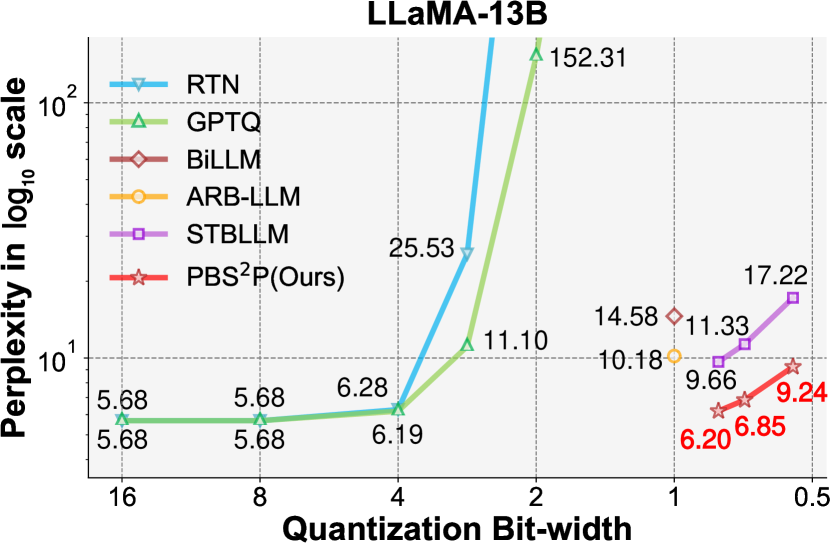
Figure 1: Perplexity of LLaMA-13B on WikiText2 under different bit-widths. Round-to-nearest (RTN) and GPTQ experience a sharp increase in perplexity at ultra-low bit-widths. While promising binarization methods, like BiLLM, ARB-LLM, and STBLLM, still exhibit a significant performance gap compared to full-precision models, our PBS²P substantially narrows this gap.

The compression of LLMs can be broadly classified into several approaches, including weight quantization (Lin et al., 2024; Frantar et al., 2023), low-rank factorization (Zhang et al., 2024; Yuan et al., 2023), network pruning (Sun et al., 2024; Frantar & Alistarh, 2023), and knowledge distillation (Zhong et al., 2024; Gu et al., 2024). Binarization, as an extreme form of quantization, can compress a model to 1 bit, significantly reducing its memory footprint. Currently, many binarization methods adopt Post-Training Quantization (Huang et al., 2024; Li et al., 2025; Dong et al., 2025), which simplifies computation by eliminating backpropagation, accelerating binarization and improving practicality. Specifically, BiLLM (Huang et al., 2024) proposes a residual approximation strategy to improve 1-bit LLMs, while ARB-LLM (Li et al., 2025) uses an alternating refined method to align the distribution between binarized and full-precision weights. STBLLM (Dong et al., 2025) pushes the limits by compressing LLMs to less than 1-bit precision. However, binarized LLMs still exhibit redundancy, which can be further reduced for even greater compression.

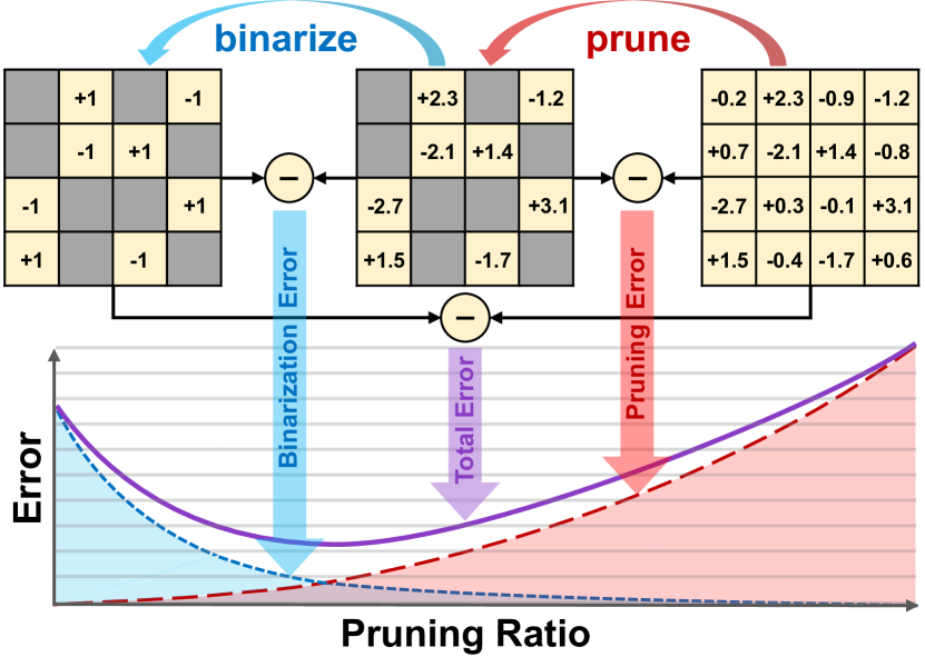
Figure 2: Total error curves with varying pruning ratios. The total error reaches its minimum at an optimal pruning ratio.

Pruning (LeCun et al., 1989) is a promising approach to further reduce redundancy in binarized models. However, conventional structured pruning (Ma et al., 2023; Ashkboos et al., 2024; Xia et al., 2024; An et al., 2024) often causes significant performance degradation in LLMs. Unstructured pruning (Dong et al., 2024) struggles with hardware acceleration and storage efficiency. Semi-structured pruning (Frantar & Alistarh, 2023; Sun et al., 2024; Dong et al., 2025), effectively reduces model redundancy, offering a balanced trade-off between performance and hardware efficiency. Yet, directly combining binarization and semi-structured pruning results in a substantial performance drop. Moreover, a significant challenge is how to effectively select pruning elements in LLMs to enhance the pruning efficiency and effectiveness, while preserving model performance.

To address those challenges, we propose a Progressive Binarization with Semi-Structured Pruning (PBS²P) for LLMs, which achieves significant model compression while maintaining strong performance (see Figure 1). We first propose Stepwise semi-structured Pruning with Binarization Optimization (SPBO) method. SPBO prunes a subset of elements at each step and optimizes the binarized parameters simultaneously. This approach effectively minimizes the total error introduced by both pruning and binarization. Next, we design a Coarse-to-Fine Search (CFS) method to select pruning elements more effectively. In the coarse-stage, the pruning ratio for each layer is determined based on layer redundancy. In the fine-stage, we use a Hessian-based metric to identify the specific elements to prune, with the pruning ratio guiding the selection process. Surprisingly, we find that with our SPBO method, the total error at an appropriate pruning ratio can be even lower than that of binarization alone. Figure 2 shows the relationship between total error and pruning ratio, demonstrating the effectiveness of our method in reducing the total error.

Extensive experiments show that PBS²P achieves SOTA performance across multiple LLM families, outperforming existing binary PTQ methods on various evaluation metrics. As illustrated in Figure 1, on the WikiText-2 (Merity et al., 2017) evaluation metric, PBS²P achieves a perplexity of 6.20 on LLaMA-13B (Touvron et al., 2023a) with an average bit-width of only 0.8 bits, compared to 5.47 for the full-precision model. PBS²P significantly narrows the gap between binarized and full-precision models.

Our key contributions can be summarized as follows:

• We propose a novel framework, PBS²P, which integrates binarization and semi-structured pruning seamlessly for effective LLM compression.

• We propose a Stepwise semi-structured Pruning with Binarization Optimization (SPBO) method, significantly reducing the total error from pruning and binarization, even below that of the no-pruning scenario.

• We design a Coarse-to-Fine Search (CFS) method to select pruning elements, which effectively reduces redundancy while maintaining performance.

• Extensive experiments demonstrate that PBS²P outperforms SOTA binary PTQ methods, significantly narrowing the performance gap between binarized models and their full-precision counterparts.

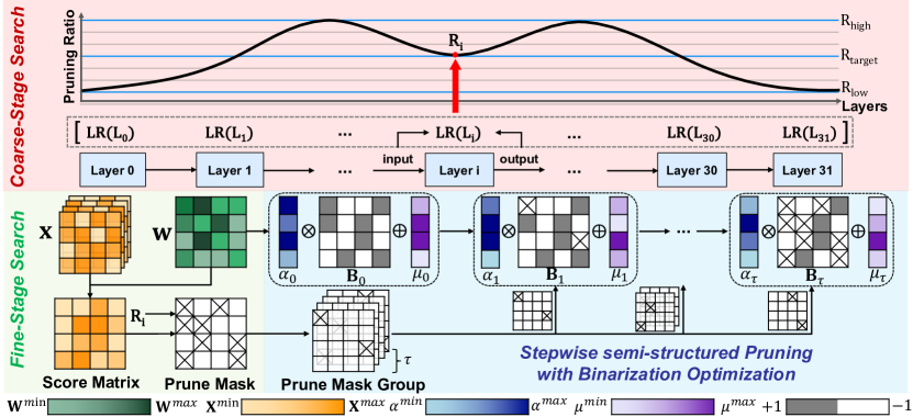
Figure 3: Overview of our PBS²P framework. Coarse-Stage Search: using the LR score to assign pruning ratios to each layer. Fine-Stage Search: searching the elements to be pruned based on the Hessian-based score matrics. Stepwise semi-structured Pruning with Binarization Optimization : stepwise pruning with alternating optimization of binarized parameters.

2 Related Works

2.1 Weight Quantization

Quantization compresses full-precision parameters into lower-bit representations, reducing both computation and storage demands. Current quantization methods for LLMs are mainly divided into Quantization-Aware Training (QAT) and Post-Training Quantization (PTQ). QAT (Liu et al., 2024; Chen et al., 2024; Du et al., 2024) integrates quantization during the training phase to enhance low-bit weight representations. However, due to the enormous parameter number, retraining becomes excessively expensive and inefficient for LLMs. PTQ, as it directly applies quantization to the model weights without retraining, making it faster and less resource-demanding. Recent methods, like ZeroQuant (Yao et al., 2022) and BRECQ (Li et al., 2021), improve quantization accuracy by incorporating custom quantization blocks and group labels. While GPTQ (Frantar et al., 2023) and QuIP (Chee et al., 2024) use second-order error compensation to reduce quantization errors.

Binarization, as the most extreme form of quantization, reduces model parameters to a single bit (±1). Prominent methods, like Binary Weight Network (BWN) (Rastegari et al., 2016) and XNOR-Net (Rastegari et al., 2016), focus on binarizing the weights, with XNOR-Net (Rastegari et al., 2016) also binarizing activations. In the context of LLM binarization, BitNet (Wang et al., 2023), OneBit (Xu et al., 2024), and BinaryMoS (Jo et al., 2024) adopt the QAT framework, while BiLLM (Huang et al., 2024), ARB-LLM (Li et al., 2025), and STBLLM(Dong et al., 2025) use PTQ combined with residual approximation. Our work focuses on the binary PTQ method, achieving substantial improvements over existing SOTA binary PTQ methods.

2.2 LLM Pruning

Pruning is a widely used technique for compressing neural networks by removing less significant parameters, reducing the number of active weights. This results in sparse networks that are more efficient in memory, computation, and size. In LLMs, pruning methods are generally divided into structured, unstructured, and semi-structured approaches. Structured pruning (Ma et al., 2023; Ashkboos et al., 2024; Xia et al., 2024; An et al., 2024) eliminates entire structured model components to improve efficiency. However, this approach can lead to substantial performance degradation, often requiring retraining to restore lost functionality. Unstructured pruning (Dong et al., 2024), removes weight elements individually based on their importance, maintaining high performance even at higher sparsity levels, but the resulting sparsity patterns are not hardware-efficient. Semi-structured pruning strikes an optimal balance by keeping regular sparsity patterns, such as $N$:$M$ sparsity, which is optimized for hardware, as seen in methods like SparseGPT (Frantar & Alistarh, 2023), Wanda (Sun et al., 2024), and STBLLM (Dong et al., 2025). Our approach leverages semi-structured pruning with $N$:$M$ sparsity, aiming to minimize performance degradation while maintaining hardware efficiency.

2.3 Integration of Pruning and Quantization

The combination of pruning and quantization has been extensively explored for neural network compression. Pruning reduces parameter counts, while quantization minimizes parameter precision. For example, Deep Compression (Han et al., 2016) integrates pruning, quantization, and Huffman coding to reduce storage requirements for deep neural networks. Later studies (Tung & Mori, 2018; Yang et al., 2020; Hu et al., 2021) have developed methods to combine pruning and quantization in parallel to optimize compression strategies. In extreme cases like binarization, methods such as STQ-Nets (Munagala et al., 2020), BNN Pruning  (Li & Ren, 2020), and BAP (Wang et al., 2021) combine these techniques to achieve high compression ratios and speedups. STBLLM (Dong et al., 2025) uses the structural binary method to compress LLMs to less than 1-bit precision, further advancing model compression and efficiency. However, simply combining pruning with binarization still leads to significant model degradation in LLMs. Therefore, we propose a new framework, PBS²P, which aims to reduce the combined errors of pruning and binarization, improving the performance of the compressed model.

3 Method

In this section, We first introduce the fundamentals of binarization and semi-structured pruning in Section 3.1. We then propose two novel methods: Stepwise semi-structured Pruning with Binarization Optimization (SPBO) and Coarse-to-Fine Search (CFS), which are elaborated in Sections 3.2 and 3.3, respectively. In Section 3.4, we provide the pipeline of PBS²P (Fig. 3) and its implementation details.

3.1 Preliminary

Binarization.  First, let’s briefly review the process of standard binarization (Rastegari et al., 2016). Binarization begins by performing a row-wise redistribution on the full-precision matrix $\mathbf{W}\in\mathbb{R}^{n\times m}$ , resulting in a matrix $\widetilde{\mathbf{W}}\in\mathbb{R}^{n\times m}$ with a mean of 0:

$$\widetilde{\mathbf{W}}=\mathbf{W}-\mu,\quad\text{where}\,\mu=\frac{1}{m}\sum_{j=1}^{m}\mathbf{W}_{.j}\,.$$ (1)

Then, the objective of binarization is defined as follows:

$$\mathop{\arg\min}\limits_{\alpha,\mathbf{B}}||\widetilde{\mathbf{W}}-\alpha\mathbf{B}||^{2}_{F},$$ (2)

where $\alpha\in\mathbb{R}^{n}$ represents the scaling factor applied to each row, and $\mathbf{B}\in\{+1,-1\}^{n\times m}$ is the binary matrix. Under the binarization objective (Equation 2), the optimal solutions for $\alpha$ and $\mathbf{B}$ are given by $\alpha=\frac{1}{m}\sum_{j=1}^{m}|\widetilde{\mathbf{W}}_{.j}|$ and $\mathbf{B}=\operatorname{sign}(\widetilde{\mathbf{W}})$, respectively (Huang et al., 2024).

N:M Sparsity.  $N$:$M$ sparsity is a form of semi-structured pruning that strikes a balance between model compression and hardware efficiency. Unlike unstructured pruning, which removes arbitrary weights and leads to irregular sparsity patterns that are difficult to accelerate on modern hardware, $N$:$M$ sparsity enforces a structured constraint by retaining exactly $N$ nonzero elements out of every $M$ consecutive weights (Frantar & Alistarh, 2023; Sun et al., 2024; Dong et al., 2025). A common setting, such as 2:4 sparsity, ensures that only two out of every four weights are retained in a layer, effectively reducing the number of parameters while maintaining computational efficiency. Due to this structured constraint, $N$:$M$ sparsity enables efficient deployment on NVIDIA Ampere architecture (Nvidia, 2020), leveraging hardware acceleration capabilities.

3.2 Stepwise Semi-Structured Pruning with Binarization Optimization

We first define the total error $\mathcal{L}_{2}$ for binarization and semi-structured pruning as follows:

$$\mathcal{L}_{2}=||\mathbf{W}\mathbf{X}-(\mathbf{M}_{\text{p}}\odot\mathbf{\widehat{W}})\mathbf{X}||_{F}^{2},$$ (3)

where $\mathbf{X}$ denotes the calibration data, $\mathbf{M}_{\text{p}}$ denotes the pruning mask. Optimizing both of the pruning mask $\mathbf{M}_{\text{p}}$ and binarized parameters $\mathbf{\widehat{W}}$ simultaneously is an NP-hard problem. Therefore, we focus on the optimization of binarized parameters with a fixed mask. The selection of the pruning mask will be elaborated in Section 3.3.

N:M Sparsity Pruning Mask Group.  We apply $N$:$M$ sparsity, a semi-structured pruning method to prune the model. We segment the overall pruning mask into $M-N$ sub-pruning masks, as illustrated in Figure 4. In the $N$:$M$ sparsity scheme, every $M$ consecutive elements will have $M-N$ elements pruned, retaining $N$ elements. The $M-N$ pruned elements are distributed across $M-N$ pruning masks. This process is given by the following formula:

$$\mathbf{M}_{\text{p}}=\bigcup_{i=1}^{M-N}\mathbf{M}_{\text{p}}^{i}.\vskip-2.84526pt$$ (4)

This way, we can distribute the optimization of the binarized parameters across each pruning step. This ensures that not too many elements are pruned at once, thus preventing the binarization difficulty from increasing. A detailed analysis of binarization difficulty and the impact of pruning on binarization can be found in the supplementary material.

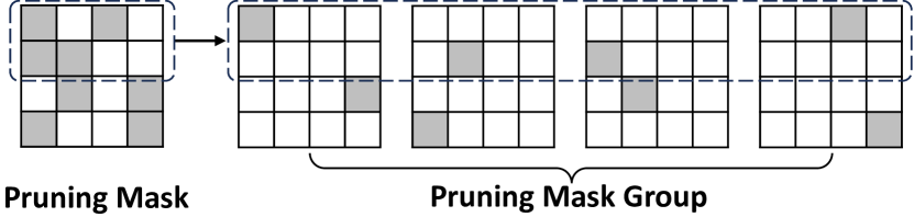
Figure 4: Illustration of the $N$:$M$ sparsity pruning mask segmentation, where the pruning mask is divided into $M-N$ sub-pruning masks, each representing a subset of the pruned elements.

Stepwise Pruning with Binarization Optimization.  Our SPBO method optimizes the binarized parameters after each pruning step, which significantly reduces $\mathcal{L}_{2}$. Inspired by ARB-LLM (Li et al., 2025), we decouple $\mathbf{X}$ and $\mathbf{W}$ to reduce computational complexity. We perform a total of $M-N$ pruning steps to achieve $N$:$M$ sparsity. Suppose we are currently performing the $k$-th pruning step, we first calculate the $k$-th pruning mask $(\mathbf{M}_{\text{p}})_{k}$:

$$(\mathbf{M}_{\text{p}})_{k}=\bigcup_{i=1}^{k}\mathbf{M}_{\text{p}}^{i}.$$ (5)

Then, we obtain the binarized matrix $\mathbf{B}_{k}$ and full-precision weight matrix $\mathbf{W}_{k}$ after the $k$-th pruning round:

$$\mathbf{B}_{k}=\mathbf{B}\odot(\mathbf{M}_{\text{p}})_{k},\,\,\,\mathbf{W}_{k}=\mathbf{W}\odot(\mathbf{M}_{\text{p}})_{k}.$$ (6)

We begin optimizing the binarized parameters $\mu$ and $\alpha$. First, we set $\partial\mathcal{L}_{2}/\partial\mu=0$ to adjust $\mu$ during the $k$-th pruning:

$$\mu_{k}=\frac{\mathbf{1}^{\top}\mathbf{S}(\mathbf{W}_{k}-\alpha_{k-1}\mathbf{B}_{k})^{\top}}{\mathbf{1}^{\top}\mathbf{S}\mathbf{1}},$$ (7)

where $\mathbf{S}=\sum\nolimits_{b}\mathbf{X}_{b}^{T}\mathbf{X}_{b}$ represents the decoupled calibration data $\mathbf{X}$. Then, we adjust $\alpha$ by setting $\partial\mathcal{L}_{2}/\partial\alpha=0$:

$$\alpha_{k}=\frac{\operatorname{diag}(\mathbf{B}_{k}\mathbf{S}(\mathbf{W}_{k}-\mu_{k})^{\top})}{\operatorname{diag}(\mathbf{B}_{k}\mathbf{S}\mathbf{B}_{k}^{\top})}.$$ (8)

During the $k$-th pruning round, we can alternately update $\mu_{k}$ and $\alpha_{k}$ to further reduce $\mathcal{L}_{2}$. We perform total $M-N$ steps of pruning until all pruning elements are removed. For the detailed procedure of the SPBO method, refer to Algorithm 1. The detailed derivation of optimizing $\mu$ and $\alpha$ can be found in the supplementary material.

Algorithm 1 SBPO algorithm: More details of each function are shown in supplementary material

func $\operatorname{SPBO}$($\mathbf{W}$, $\mathbf{M}_{\text{p}}$, $\mathbf{X}$ ,$T$)
Input: $\mathbf{W}\in\mathbb{R}^{n\times m}$ - full-precision weight
    $\mathbf{M}_{\text{p}}\in\mathbb{R}^{n\times m}$ - pruning mask
    $\mathbf{X}\in\mathbb{R}^{B\times L\times m}$ - calibration data
    $T$ - binarized parameter optimization steps
Output: $\mathbf{\widehat{W}}\in\mathbb{R}^{n\times m}$

1: $\mathbf{S}\coloneqq\operatorname{X2S}(\mathbf{X})$ $\triangleright$ decouple $\mathbf{W}$ and $\mathbf{X}$

2: $\widehat{\mathbf{W}},\alpha,\mathbf{B},\mu\coloneqq\operatorname{binary}(\mathbf{W})$

3: $\textbf{M}_{\text{group}}\coloneqq\operatorname{split\_mask}(\mathbf{M}_{\text{p}})$

4: $\mathbf{M}_{\text{k}}\coloneqq\mathbf{M}_{\text{group}}[0]$

5: for $\textbf{M}\text{ in }\mathbf{M}_{\text{group}}$ do

6:  $\mathbf{B}\leftarrow\mathbf{B}\odot\mathbf{M}$$\triangleright$ prune binarized matrix

7:  $\mathbf{W}\leftarrow\mathbf{W}\odot\mathbf{M}$

8:  $\mathbf{M}_{k}\leftarrow\mathbf{M}_{k}\cup\mathbf{M}$ $\triangleright$ current pruning mask

9:  for $iter=1,2,\ldots,T$ do

10:   $\mu\leftarrow\operatorname{update\_\mu}(\mathbf{S},\mathbf{W},\mathbf{B},\alpha)$$\triangleright$ update $\mu$

11:   $\alpha\leftarrow\operatorname{update\_\alpha}(\mathbf{S},\mathbf{W},\mu,\mathbf{B})$$\triangleright$ update $\alpha$

12:   $\widehat{\mathbf{W}}\leftarrow(\alpha\cdot\mathbf{B}+\mu)\odot\mathbf{M}_{k}$

13:  end for

14: end for

15: return $\mathbf{\widehat{W}}$

func $\operatorname{update\_\alpha}$ $(\mathbf{S},\mathbf{W},\mathbf{\mu},\mathbf{B})$

1: $\widetilde{\mathbf{W}}\coloneqq\mathbf{W}-\mu$

2: for $i=1,2,\ldots,n$ do

3:  for $k=1,2,\ldots,m;l=1,2,\ldots,m$ do

4:   $\mathbf{U}_{kl}\coloneqq\mathbf{B}_{ik}\widetilde{\mathbf{W}}_{il}$

5:   $\mathbf{V}_{kl}\coloneqq\mathbf{B}_{ik}\mathbf{B}_{il}$

6:  end for

7:  $num\coloneqq\sum_{k}\sum_{l}(\mathbf{S}\odot\mathbf{U})_{kl}$

8:  $den\coloneqq\sum_{k}\sum_{l}(\mathbf{S}\odot\mathbf{V})_{kl}+\epsilon$

9:  $\alpha_{i}\coloneqq\frac{num}{den}$$\triangleright$ refined $\alpha$

10: end for

11: return $\alpha$

func $\operatorname{update\_\mu}$ $(\mathbf{S},\mathbf{W},\mathbf{B},\alpha)$

1: for $i=1,2,\ldots,n$ do

2:  for $k=1,2,\ldots,m;l=1,2,\ldots,m$ do

3:   $\mathbf{P}_{kl}\coloneqq\mathbf{W}_{ik}-\alpha_{i}\mathbf{B}_{il}$

4:  end for

5:  $num\coloneqq\sum_{k}\sum_{l}(\mathbf{S}\odot\mathbf{P})_{kl}$

6:  $den\coloneqq\sum_{k}\sum_{l}\mathbf{S}_{kl}+\epsilon$

7:  $\mu_{i}\coloneqq\frac{num}{den}$$\triangleright$ refined $\mu$

8: end for

9: return $\mu$

func $\operatorname{binary}$ $(\mathbf{W})$

1: $\mu\coloneqq\frac{1}{m}\sum_{j=1}^{m}\mathbf{W}_{.j}$

2: $\widetilde{\mathbf{W}}\coloneqq\mathbf{W}-\mu$$\triangleright$ row-wise redistribution

3: $\alpha\coloneqq\frac{1}{m}\sum_{j=1}^{m}|\widetilde{\mathbf{W}}_{.j}|$$\triangleright$ row-wise scaling factor

4: $\mathbf{B}\coloneqq\operatorname{sign}(\widetilde{\mathbf{W}})$

5: $\mathbf{\widehat{W}}\coloneqq\alpha\cdot\mathbf{B}+\mu$$\triangleright$ binarized output

6: return $\mathbf{\widehat{W}},\alpha,\mathbf{B},\mu$

func $\operatorname{X2S}$ $(\mathbf{X})$

1: for $b=1,2,\ldots B$ do

2:  for $k=1,2,\ldots,m;l=1,2,\ldots,m$ do

3:   $\mathbf{S}_{kl}=\sum_{b}\sum_{i}(\mathbf{X}_{b})_{ik}(\mathbf{X}_{b})_{il}$

4:  end for

5: end for

6: return $\mathbf{S}$

3.3 Coarse-to-Fine Search

Coarse-Stage: Pruning Ratio Allocation.  Inspired by Dumitru et al. (2024), we use the Layer Redundancy (LR) score to measure the importance of different layers:

$$\text{LR}(\textbf{L}_{i})=\frac{\mathbf{I}_{i}\cdot\mathbf{O}_{i}}{\|\mathbf{I}_{i}\|_{2}\|\mathbf{O}_{i}\|_{2}},$$ (9)

where $\mathbf{I_{i}}$ denotes the input of the $i$-th layer $\mathbf{L}_{i}$, and $\mathbf{O_{i}}$ denotes the output of the same layer. A higher LR score indicates greater redundancy within the layer, meaning that the importance of this layer is lower. We take the different importance of layers into account when selecting pruning elements. We first rank the layers of the model from low to high based on the LR score, with $k_{i}$ denoting the rank of the i-th layer. The corresponding pruning parameter $N_{i}$ for the i-th layer is then assigned using the following formula:

$$N_{i}=\left\lfloor N_{\text{high}}-\left(N_{\text{high}}-N_{\text{low}}\right)\cdot\frac{k_{i}-1}{L-1}+\frac{1}{2}\right\rfloor,$$ (10)

where $L$ represents the total number of layers in the model. $N_{\text{high}}$ is the maximum pruning parameter, and $N_{\text{low}}$ is the minimum pruning parameter. We define the target pruning parameter $N_{\text{target}}$ as the average pruning parameter across the entire model. In our experiments, $N_{\text{high}}$ is set to $N_{\text{target}}+1$, while $N_{\text{low}}$ is set to $N_{\text{target}}-1$.

Table 1: Perplexity comparison of RTN, GPTQ, BiLLM, ARB-LLM, STBLLM, and PBS²P on the LLaMA and OPT families. The evaluation results demonstrate the perplexity performance on the Wikitext2 dataset across various model sizes.

Settings			LLaMA-1				LLaMA-2		LLaMA-3	OPT
Method	#Block	W-Bits	7B	13B	30B	65B	7B	13B	8B	1.3B	2.7B	30B
FP16	-	16	5.68	5.09	4.1	3.53	5.47	4.88	6.14	14.62	12.47	9.56
1-13 RTN	-	3	25.54	11.40	14.89	10.59	5.4e2	10.68	2.2e3	1.3e4	1.6e4	1.6e3
GPTQ	128	3	8.63	5.67	4.87	4.17	6.44	5.46	18.68	16.45	13.61	9.71
RTN	-	2	1.1e5	5.7e4	2.7e4	2.0e4	1.8e4	5.1e4	1.3e6	1.1e4	9.5e3	1.7e5
GPTQ	128	2	1.3e2	20.46	15.29	8.66	52.22	23.63	1.4e3	1.2e2	59.53	13.04
1-13 RTN	-	1	1.7e5	1.4e6	1.5e4	6.5e4	1.6e5	4.8e4	1.4e6	1.7e4	3.7e4	6.5e3
GPTQ	128	1	1.6e5	1.3e5	1.0e4	2.0e4	6.0e4	2.3e4	1.1e6	8.7e3	1.2e4	1.4e4
BiLLM	128	1.11	49.79	14.58	9.90	8.37	32.31	21.35	55.80	69.05	48.61	13.86
ARB-LLM	128	1.11	14.03	10.18	7.75	6.56	16.44	11.85	27.42	26.63	19.84	11.12
1-13 STBLLM	128	0.80	15.03	9.66	7.56	6.43	13.06	11.67	33.44	29.84	17.02	12.80
STBLLM	128	0.70	19.48	11.33	9.19	7.91	18.74	13.26	49.12	33.01	20.82	14.38
STBLLM	128	0.55	31.72	17.22	13.43	11.07	27.93	20.57	253.76	45.11	30.34	18.80
1-13 PBS2P	128	0.80	7.36	6.20	5.21	4.60	7.17	6.27	10.75	23.72	18.32	10.50
PBS2P	128	0.70	8.09	6.85	5.78	5.09	8.00	6.89	12.29	27.10	20.17	10.82
PBS2P	128	0.55	10.78	9.24	7.19	6.39	10.64	8.68	17.45	44.53	27.42	11.87

Fine-Stage: Selecting Pruning Elements.  Once the pruning parameter $N$ is assigned in the coarse-stage, we proceed to search for the specific pruning elements within each layer. Inspired by BiLLM (Huang et al., 2024), we utilize the Hessian matrix to evaluate the importance of elements in the weight matrix. The Hessian-based score matrix is defined as $s_{i}=\frac{w_{i}^{2}}{\left[\mathbf{H}^{-1}\right]_{ii}^{2}}$, where $\mathbf{H}$ denotes the Hessian matrix of the layer, and $w_{i}$ represents the original value of each element. Based on the given $N$:$M$ ratio and the corresponding $s_{i}$ values, we select the top $N$ elements with the largest $s_{i}$ values from every $M$ consecutive elements to retain. The other $M-N$ elements are selected for pruning.

3.4 PBS²P Pipeline

PBS²P Workflow.  PBS²P quantizes all the linear layers in each transformer block of the LLM. We first perform the coarse-stage search to determine the pruning ratio for different transformer blocks. Then we proceed with the fine-stage search for pruning elements layer by layer and perform stepwise semi-structured pruning with binarization optimization. Following BiLLM (Huang et al., 2024), ARB-LLM (Li et al., 2025), and STBLLM (Dong et al., 2025), we divide the weights into salient and non-salient parts. For the salient part, we employ residual binarization. For the non-salient part, similar to STBLLM, we use two split points $p$ to divide the non-salient weights into three segments, each binarized separately. It ensuring that the total parameter count remains the same for a fair comparison. We adopt the block-wise compensation strategies from GPTQ (Frantar et al., 2023) and OBC (Frantar & Alistarh, 2022) to further mitigate quantization error.

Average Bits.  Following BiLLM (Huang et al., 2024) and STBLLM (Dong et al., 2025), we add extra bits while pruning the redundant or less important weights. The weight parameters and additional hardware overhead are as follows:

$$\left\{\begin{array}[]{lr}N_{\text{param}}=\left[2\times r_{\text{salient}}+(1-r_{\text{salient}})\right]\times\frac{N}{M},\\ N_{\text{storing}}=2+\dfrac{1}{b_{\text{size}}},\\ \end{array}\right.$$ (11)

where $r_{\text{salient}}$ represents the proportion of salient weights, $N$:$M$ denotes the predefined pruning parameters for the entire model, and $b_{\text{size}}$ indicates the block size used in OBC compensation, with 2 bits reserved to mark the division between salient and non-salient weights. Our parameter settings and $N$:$M$ configuration are identical to our main comparison method STBLLM. We have the same bit-width with STBLLM, ensuring a fair comparison.

4 Experiments

4.1 Settings

All experiments are performed using PyTorch (Paszke et al., 2019b) and Huggingface (Paszke et al., 2019a) on a single NVIDIA A800-80GB GPU. Following the work of Frantar et al. (2023), Huang et al. (2024), and Li et al. (2025), we use 128 samples from the C4 (Raffel et al., 2020) dataset for calibration. Since PBS²P is an efficient PTQ framework, it eliminates fine-tuning, enabling completion through a single process combining binarization and pruning.

Models and Datasets.  We conduct extensive experiments on the LLaMA (Touvron et al., 2023a), LLaMA-2 (Touvron et al., 2023b), and LLaMA-3 (Dubey et al., 2024) families and the OPT family (Zhang et al., 2022). To evaluate the effectiveness of PBS²P, we measure the perplexity of LLM’s outputs on WikiText2 (Merity et al., 2017), PTB (Marcus et al., 1994), and C4 (Raffel et al., 2020). Moreover, we also evaluate the accuracy for 7 zero-shot QA datasets: ARC-c (Clark et al., 2018), ARC-e (Clark et al., 2018), BoolQ (Clark et al., 2019), Hellaswag (Zellers et al., 2019), OBQA (Mihaylov et al., 2018), RTE (Chakrabarty et al., 2021), and Winogrande (Sakaguchi et al., 2020).

Table 2: Accuracies (%) for 7 zero-shot tasks from semi-structured binarized LLaMA-1-13B, LLaMA-2-13B, and LLaMA-1-30B with STBLLM and PBS²P. We compare the accuracies under the same $N$:$M$ settings.

Models	Method	W-Bits	Winogrande	OBQA	Hellaswag	Boolq	ARC-e	ARC-c	RTE	Average
	FP16	16	72.69	33.20	59.91	77.89	77.40	46.42	70.40	63.80
2-11	STBLLM	0.80	65.98	36.20	63.67	65.38	68.86	34.04	56.68	55.83
LLaMA-1-13B	STBLLM	0.55	63.06	34.80	52.65	62.48	56.90	28.33	52.71	50.13
2-11	PBS2P	0.80	72.77	31.00	54.80	74.71	74.37	42.32	68.23	59.74
	PBS2P	0.55	69.30	26.80	46.83	71.56	65.70	32.68	55.96	52.69
	full-precision	16	72.22	35.20	60.03	80.55	79.42	48.38	65.34	65.00
2-11	STBLLM	0.80	63.93	37.00	57.76	71.53	60.56	31.99	54.15	53.85
LLaMA-2-13B	STBLLM	0.55	55.88	29.40	44.03	64.31	48.86	26.54	52.71	45.96
2-11	PBS2P	0.80	72.45	31.00	54.43	80.61	74.28	42.75	59.21	59.24
	PBS2P	0.55	69.85	27.00	47.75	75.50	69.19	35.58	62.82	55.38
	full-precision	16	75.77	36.00	63.37	82.69	80.30	52.90	67.15	67.40
2-11	STBLLM	0.80	71.59	41.00	69.85	77.37	71.55	41.3	48.01	60.10
LLaMA-1-30B	STBLLM	0.55	64.01	34.60	56.46	63.06	60.86	31.48	51.99	51.78
2-11	PBS2P	0.80	75.93	35.00	59.45	82.14	79.29	47.95	63.18	63.28
	PBS2P	0.55	72.14	31.20	53.00	79.76	73.99	41.13	69.31	60.08

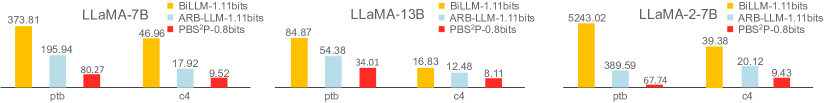
Figure 5: BiLLM, ARB-LLM, and PBS²P performed on the PTB and c4 datasets, mainly on LLaMA-7B, LLaMA-13B, and LLaMA-2-7B, and we found that PBS²P at 0.8 bits outperforms other methods at 1.11 bits.

Baselines.  We mainly compare our PBS²P with STBLLM (Dong et al., 2025), a structural binary PTQ framework designed for compressing LLMs to precisions lower than 1-bit. We implement PBS²P with a block size set to 128. We compare the results of PBS²P with STBLLM under the same $N$:$M$ settings (e.g., 4:8, 5:8, 6:8). Previous low-bit methods like ARB-LLM (Li et al., 2025), BiLLM (Huang et al., 2024), GTPQ (Frantar et al., 2023) and vanilla RTN are also selected for comparison.

4.2 Main Results

We perform a comprehensive comparison of different LLM families (like LLaMA and OPT) with various model sizes. To keep fairness, We follow STBLLM (Dong et al., 2025) to report the average bit-width of all methods, where our methods have the same bit-width as STBLLM.

Results on LLaMA Family. As shown in Table 1, the models using RTN and GPTQ methods find it hard to maintain model performance at 1-bit precision. BiLLM achieves a satisfactory perplexity of 1.11 bits but performs worse than ARB-LLM at the same bit-width. At sub-1-bit precision, PBS²P surpasses STBLLM and significantly reduces perplexity at the same bit-width across model sizes from 7B to 65B. For instance, PBS²P achieves a substantial improvement over STB-LLM on LLaMA-1-7B, with perplexity dropping from 31.72 to 10.78, a reduction of approximately 66.0%, in the extreme case of 4:8 structured binarization, where half of the parameters are pruned.

Furthermore, PBS²P, with a precision of 0.8 bits, outperforms both RTN at 3 bits, GPTQ at 2 bits, BiLLM and ARB-LLM at 1.11 bits, and STBLLM at 0.8 bits in terms of perplexity across all model sizes. Those comparisons show that our PBS²P achieves a better trade-off between bit precision and performance. It is worth noting that PBS²P outperforms GPTQ at 3 bits on LLaMA 1-7B and LLaMA 3-8B. We extend perplexity evaluation to the PTB and C4 datasets. Figure 5 shows the performance of the LLaMA-7B, LLaMA-13B, and LLaMA-2-7B models. PBS²P continues to achieve a leading edge in performance while operating at a relatively lower bit-width compared to other methods.

Results on OPT Family.  We extend our experiments to the OPT family (1.3B to 30B) under sub-1-bit PTQ settings, similar to the setup for LLaMA family. As shown in Table 1, PBS²P continues to outperform STBLLM across most of the models and $N$:$M$ structured binarization configurations. More results are provided in the supplementary material.

4.3 Zero-Shot Results

To provide a more thorough evaluation of binary LLMs, we extend our experiments to 7 zero-shot datasets and test on models from the LLaMA family: LLaMA-1-13B, LLaMA-2-13B, and LLaMA-1-30B. Each model is evaluated across various compression methods, including full-precision, STBLLM (6:8), STBLLM (4:8), PBS²P (6:8), and PBS²P (4:8). As shown in Table 2, models compressed with PBS²P significantly outperform those compressed with STBLLM in terms of average accuracy. Such comparisons demonstrate that PBS²P provides a more effective solution for compressing LLMs to less than 1-bit.

Table 3: Ablation study on LLaMA-7B, where all PBS²P is applied an $N$:$M$ sparsity of 4:8. Results are measured by perplexity on the Wikitext2 and C4 datasets. Our results are highlighted in bold.

SPBO Strategy	Wikitext2$\downarrow$	C4$\downarrow$
✗	14.43	16.76
✓	10.78	13.06

(a) Ablation for SPBO Strategy.

Group Size	64	128	256	512
Wikitext2$\downarrow$	10.24	10.78	11.20	11.91
C4$\downarrow$	12.50	13.06	13.68	14.51

(b) Ablation for Group Size

Coarse-Stage Search	Metric	Wikitext2$\downarrow$	C4$\downarrow$
✗	—	11.55	13.94
✓	RI	14.43	16.76
✓	LR	10.78	13.06

(c) Ablation for Metric in Coarse-Stage Search (CSS)

Prune Type	Hardware-friendly	Wikitext2$\downarrow$	C4$\downarrow$
Structured	✓	621.16	400.50
Unstructured	✗	8.54	10.95
Semi-Structured	✓	10.78	13.06

(d) Ablation for Pruning Type

Metric	Random	Magnitude	Wanda	SI	Ours
Wikitext2$\downarrow$	7,779.28	38.90	10.89	196.61	10.78
C4$\downarrow$	6,797.09	24.47	13.16	148.85	13.06

(e) Ablation for Metric in Fine-Stage Search

#Split Points	1	2	3
Wikitext2$\downarrow$	13.41	10.78	10.55
C4$\downarrow$	15.97	13.06	12.83

(f) Ablation for Number of Split Points

4.4 Ablation Study

Ablation for SPBO Strategy.  To validate the effectiveness of our SPBO strategy, we provide the performance of PBS²P with and without its application. As shown in Table 3a, the performance of SPBO surpasses that of the vanilla pruning followed by binarization approach. In the vanilla method, pruning is done in a single step, where all elements are pruned simultaneously, and binarization is applied to the remaining elements afterward. However, the vanilla approach makes it hard to effectively minimize the combined errors. These results demonstrate the performance improvement achieved through our SPBO strategy.

Ablation for Group Size.  Table 3b presents the results of our ablation study on the group size configuration. It indicates that a smaller group size, meaning finer-grained grouping, leads to better performance. However, this also comes with increased computational and storage costs. To strike a balance between performance and resource efficiency, we select a group size of 128.

Ablation for Metric in Coarse-Stage Search.  Table 3c shows the performance of the coarse-stage search under three conditions: without the coarse-stage search, using the relative importance (RI) metric from STBLLM, and applying our layer redundancy (LR) score. The results reveal that using the RI metric causes a performance drop compared to the baseline without coarse-stage search. In contrast, applying our LR score leads to a clear improvement, demonstrating not only the effectiveness of our coarse-stage search but also the superiority of the LR score metric.

Ablation for Pruning Type.  In Table 3d, we present the impact of different pruning types on the results, comparing structured pruning, unstructured pruning, and semi-structured pruning under the same pruning ratio (50%). For semi-structured pruning, we use an $N$:$M$ sparsity of 4:8, while for structured pruning, we apply column pruning. For unstructured pruning, we perform elementwise pruning based on weight importance. Semi-structured pruning outperforms structured pruning for LLM compression. It also maintains hardware-friendliness while achieving performance levels similar to unstructured pruning. This demonstrates that semi-structured pruning strikes a good trade-off between hardware efficiency and model performance.

Ablation for Metric in Fine-Stage Search.  The Table 3e presents the performance of different pruning metrics in the fine-stage search. We compare several metrics, including random selection, magnitude-based selection, Wanda, SI, and our Hessian-based metric. The experimental results demonstrate that our metric significantly outperforms both random selection and magnitude-based pruning, achieving superior performance compared to Wanda and SI, thereby highlighting the effectiveness of our approach.

Ablation for Number of Split Points.  We use a grouping strategy to quantize non-salient weights, where a split point $p$ is used to group the non-salient weights. Table 3f shows the impact of different numbers of split points on performance. From the table, we can see that as the number of split points increases, the model performance improves. However, an increase in the number of split points also leads to higher computational and storage demands. As a result, we choose the number of split points as 2, which strikes a balance between performance and resource requirements. This choice ensures a fair comparison across methods.

5 Conclusions

In this work, we propose a progressive binarization with semi-structured pruning (PBS²P) method for LLM compression. We propose SPBO, a stepwise semi-structured pruning with binarization optimization, which prunes a subset of elements at each step while simultaneously optimizing the binarized parameters. SPBO effectively reduces total errors from pruning and binarization. Additionally, we propose the coarse-to-fine search (CFS) method to improve pruning element selection, further enhancing compression efficiency. Extensive experiments show that PBS²P outperforms SOTA binary PTQ methods, achieving superior accuracy across various LLM families and metrics. Our work offers an effective solution for deploying LLMs on resource-constrained devices while maintaining strong performance and introduces a new perspective to combining compression techniques for extreme LLM compression.

References

- An et al. (2024) An, Y., Zhao, X., Yu, T., Tang, M., and Wang, J. Fluctuation-based adaptive structured pruning for large language models. In AAAI, 2024.
- Ashkboos et al. (2024) Ashkboos, S., Croci, M. L., Nascimento, M. G. d., Hoefler, T., and Hensman, J. Slicegpt: Compress large language models by deleting rows and columns. In ICLR, 2024.
- Chakrabarty et al. (2021) Chakrabarty, T., Ghosh, D., Poliak, A., and Muresan, S. Figurative language in recognizing textual entailment. arXiv preprint arXiv:2106.01195, 2021.
- Chee et al. (2024) Chee, J., Cai, Y., Kuleshov, V., and De Sa, C. M. Quip: 2-bit quantization of large language models with guarantees. In NeurIPS, 2024.
- Chen et al. (2024) Chen, H., Lv, C., Ding, L., Qin, H., Zhou, X., Ding, Y., Liu, X., Zhang, M., Guo, J., Liu, X., et al. Db-llm: Accurate dual-binarization for efficient llms. arXiv preprint arXiv:2402.11960, 2024.
- Clark et al. (2019) Clark, C., Lee, K., Chang, M.-W., Kwiatkowski, T., Collins, M., and Toutanova, K. Boolq: Exploring the surprising difficulty of natural yes/no questions. In NAACL, 2019.
- Clark et al. (2018) Clark, P., Cowhey, I., Etzioni, O., Khot, T., Sabharwal, A., Schoenick, C., and Tafjord, O. Think you have solved question answering? try arc, the ai2 reasoning challenge. arXiv preprint arXiv:1803.05457, 2018.
- Dong et al. (2024) Dong, P., Li, L., Tang, Z., Liu, X., Pan, X., Wang, Q., and Chu, X. Pruner-zero: Evolving symbolic pruning metric from scratch for large language models. In ICML, 2024.
- Dong et al. (2025) Dong, P., Li, L., Zhong, Y., Du, D., Fan, R., Chen, Y., Tang, Z., Wang, Q., Xue, W., Guo, Y., et al. Stbllm: Breaking the 1-bit barrier with structured binary llms. In ICLR, 2025.
- Du et al. (2024) Du, D., Zhang, Y., Cao, S., Guo, J., Cao, T., Chu, X., and Xu, N. Bitdistiller: Unleashing the potential of sub-4-bit llms via self-distillation. In ACL, 2024.
- Dubey et al. (2024) Dubey, A., Jauhri, A., Pandey, A., Kadian, A., Al-Dahle, A., Letman, A., Mathur, A., Schelten, A., Yang, A., Fan, A., et al. The llama 3 herd of models. arXiv preprint arXiv:2407.21783, 2024.
- Dumitru et al. (2024) Dumitru, R.-G., Clotan, P.-I., Yadav, V., Peteleaza, D., and Surdeanu, M. Change is the only constant: Dynamic llm slicing based on layer redundancy. arXiv preprint arXiv:2411.03513, 2024.
- Frantar & Alistarh (2022) Frantar, E. and Alistarh, D. Optimal brain compression: A framework for accurate post-training quantization and pruning. In NeurIPS, 2022.
- Frantar & Alistarh (2023) Frantar, E. and Alistarh, D. Sparsegpt: Massive language models can be accurately pruned in one-shot. In ICML, 2023.
- Frantar et al. (2023) Frantar, E., Ashkboos, S., Hoefler, T., and Alistarh, D. Gptq: Accurate post-training quantization for generative pre-trained transformers. In ICLR, 2023.
- Gu et al. (2024) Gu, Y., Dong, L., Wei, F., and Huang, M. Knowledge distillation of large language models. In ICLR, 2024.
- Han et al. (2016) Han, S., Mao, H., and Dally, W. J. Deep compression: Compressing deep neural networks with pruning, trained quantization and huffman coding. In ICLR, 2016.
- Hu et al. (2021) Hu, P., Peng, X., Zhu, H., Aly, M. M. S., and Lin, J. Opq: Compressing deep neural networks with one-shot pruning-quantization. In AAAI, 2021.
- Huang et al. (2024) Huang, W., Liu, Y., Qin, H., Li, Y., Zhang, S., Liu, X., Magno, M., and Qi, X. Billm: Pushing the limit of post-training quantization for llms. In ICML, 2024.
- Jo et al. (2024) Jo, D., Kim, T., Kim, Y., and Kim, J.-J. Mixture of scales: Memory-efficient token-adaptive binarization for large language models. In NeurIPS, 2024.
- LeCun et al. (1989) LeCun, Y., Denker, J., and Solla, S. Optimal brain damage. In NeurIPS, 1989.
- Li & Ren (2020) Li, Y. and Ren, F. Bnn pruning: Pruning binary neural network guided by weight flipping frequency. In ISQED, 2020.
- Li et al. (2021) Li, Y., Gong, R., Tan, X., Yang, Y., Hu, P., Zhang, Q., Yu, F., Wang, W., and Gu, S. Brecq: Pushing the limit of post-training quantization by block reconstruction. In ICLR, 2021.
- Li et al. (2025) Li, Z., Yan, X., Zhang, T., Qin, H., Xie, D., Tian, J., Kong, L., Zhang, Y., Yang, X., et al. Arb-llm: Alternating refined binarizations for large language models. In ICLR, 2025.
- Lin et al. (2024) Lin, J., Tang, J., Tang, H., Yang, S., Chen, W.-M., Wang, W.-C., Xiao, G., Dang, X., Gan, C., and Han, S. Awq: Activation-aware weight quantization for on-device llm compression and acceleration. In MLSys, 2024.
- Liu et al. (2024) Liu, Z., Oguz, B., Zhao, C., Chang, E., Stock, P., Mehdad, Y., Shi, Y., Krishnamoorthi, R., and Chandra, V. Llm-qat: Data-free quantization aware training for large language models. In ACL, 2024.
- Ma et al. (2023) Ma, X., Fang, G., and Wang, X. Llm-pruner: On the structural pruning of large language models. In NeurIPS, 2023.
- Marcus et al. (1994) Marcus, M., Kim, G., Marcinkiewicz, M. A., MacIntyre, R., Bies, A., Ferguson, M., Katz, K., and Schasberger, B. The penn treebank: Annotating predicate argument structure. In HLT, 1994.
- Merity et al. (2017) Merity, S., Xiong, C., Bradbury, J., and Socher, R. Pointer sentinel mixture models. In ICLR, 2017.
- Mihaylov et al. (2018) Mihaylov, T., Clark, P., Khot, T., and Sabharwal, A. Can a suit of armor conduct electricity? a new dataset for open book question answering. In EMNLP, 2018.
- Munagala et al. (2020) Munagala, S. A., Prabhu, A., and Namboodiri, A. M. Stq-nets: Unifying network binarization and structured pruning. In BMVC, 2020.
- Nvidia (2020) Nvidia. Nvidia a100 tensor core gpu architecture, 2020.
- Paszke et al. (2019a) Paszke, A., Gross, S., Massa, F., Lerer, A., Bradbury, J., Chanan, G., Killeen, T., Lin, Z., Gimelshein, N., Antiga, L., et al. An imperative style, high-performance deep learning library. In NeurIPS, 2019a.
- Paszke et al. (2019b) Paszke, A., Gross, S., Massa, F., Lerer, A., Bradbury, J., Chanan, G., Killeen, T., Lin, Z., Gimelshein, N., Antiga, L., et al. Pytorch: An imperative style, high-performance deep learning library. In NeurIPS, 2019b.
- Raffel et al. (2020) Raffel, C., Shazeer, N., Roberts, A., Lee, K., Narang, S., Matena, M., Zhou, Y., Li, W., and Liu, P. J. Exploring the limits of transfer learning with a unified text-to-text transformer. JMLR, 2020.
- Rastegari et al. (2016) Rastegari, M., Ordonez, V., Redmon, J., and Farhadi, A. Xnor-net: Imagenet classification using binary convolutional neural networks. In ECCV, 2016.
- Sakaguchi et al. (2020) Sakaguchi, K., Le Bras, R., Bhagavatula, C., and Choi, Y. Winogrande: An adversarial winograd schema challenge at scale. In AAAI, 2020.
- Sun et al. (2024) Sun, M., Liu, Z., Bair, A., and Kolter, J. Z. A simple and effective pruning approach for large language models. In ICLR, 2024.
- Touvron et al. (2023a) Touvron, H., Lavril, T., Izacard, G., Martinet, X., Lachaux, M.-A., Lacroix, T., Rozière, B., Goyal, N., Hambro, E., Azhar, F., et al. Llama: Open and efficient foundation language models. arXiv preprint arXiv:2302.13971, 2023a.
- Touvron et al. (2023b) Touvron, H., Martin, L., Stone, K., Albert, P., Almahairi, A., Babaei, Y., Bashlykov, N., Batra, S., Bhargava, P., Bhosale, S., et al. Llama 2: Open foundation and fine-tuned chat models. arXiv preprint arXiv:2307.09288, 2023b.
- Tung & Mori (2018) Tung, F. and Mori, G. Clip-q: Deep network compression learning by in-parallel pruning-quantization. In CVPR, 2018.
- Vaswani (2017) Vaswani, A. Attention is all you need. In NeurIPS, 2017.
- Wang et al. (2023) Wang, H., Ma, S., Dong, L., Huang, S., Wang, H., Ma, L., Yang, F., Wang, R., Wu, Y., and Wei, F. Bitnet: Scaling 1-bit transformers for large language models. arXiv preprint arXiv:2310.11453, 2023.
- Wang et al. (2021) Wang, P., Li, F., Li, G., and Cheng, J. Extremely sparse networks via binary augmented pruning for fast image classification. TNNLS, 2021.
- Xia et al. (2024) Xia, M., Gao, T., Zeng, Z., and Chen, D. Sheared llama: Accelerating language model pre-training via structured pruning. In ICLR, 2024.
- Xu et al. (2024) Xu, Y., Han, X., Yang, Z., Wang, S., Zhu, Q., Liu, Z., Liu, W., and Che, W. Onebit: Towards extremely low-bit large language models. In NeurIPS, 2024.
- Yang et al. (2020) Yang, H., Gui, S., Zhu, Y., and Liu, J. Automatic neural network compression by sparsity-quantization joint learning: A constrained optimization-based approach. In CVPR, 2020.
- Yao et al. (2022) Yao, Z., Yazdani Aminabadi, R., Zhang, M., Wu, X., Li, C., and He, Y. Zeroquant: Efficient and affordable post-training quantization for large-scale transformers. In NeurIPS, 2022.
- Yuan et al. (2023) Yuan, Z., Shang, Y., Song, Y., Wu, Q., Yan, Y., and Sun, G. Asvd: Activation-aware singular value decomposition for compressing large language models. arXiv preprint arXiv:2312.05821, 2023.
- Zellers et al. (2019) Zellers, R., Holtzman, A., Bisk, Y., Farhadi, A., and Choi, Y. Hellaswag: Can a machine really finish your sentence? In ACL, 2019.
- Zhang et al. (2024) Zhang, M., Chen, H., Shen, C., Yang, Z., Ou, L., Yu, X., and Zhuang, B. Loraprune: Pruning meets low-rank parameter-efficient fine-tuning. In ACL, 2024.
- Zhang et al. (2022) Zhang, S., Roller, S., Goyal, N., Artetxe, M., Chen, M., Chen, S., Dewan, C., Diab, M., Li, X., Lin, X. V., et al. Opt: Open pre-trained transformer language models. arXiv preprint arXiv:2205.01068, 2022.
- Zhong et al. (2024) Zhong, Q., Ding, L., Shen, L., Liu, J., Du, B., and Tao, D. Revisiting knowledge distillation for autoregressive language models. In ACL, 2024.