Learning with Differentially Private (Sliced) Wasserstein Gradients

Abstract

In this work, we introduce a novel framework for privately optimizing objectives that rely on Wasserstein distances between data-dependent empirical measures. Our main theoretical contribution is, based on an explicit formulation of the Wasserstein gradient in a fully discrete setting, a control on the sensitivity of this gradient to individual data points, allowing strong privacy guarantees at minimal utility cost. Building on these insights, we develop a deep learning approach that incorporates gradient and activations clipping, originally designed for DP training of problems with a finite-sum structure. We further demonstrate that privacy accounting methods extend to Wasserstein-based objectives, facilitating large-scale private training. Empirical results confirm that our framework effectively balances accuracy and privacy, offering a theoretically sound solution for privacy-preserving machine learning tasks relying on optimal transport distances such as Wasserstein distance or sliced-Wasserstein distance.

1 Introduction

Optimal transport distances have been shown to be a powerful tool for measuring discrepancies between distributions in learning problems. Given two probabilities $P$ and $Q$ in $\mathbb{R}^{d}$, the Wasserstein distance $W_{p}(P,Q)$ is defined as the $p^{th}$ root of the cost associated to the optimal transport plan, i.e.,

$$W_{p}(P,Q)=\Bigl{(}\inf_{\pi\in\Pi(P,Q)}\ \int_{\mathbb{R}^{d}}\|x-y\|_{2}^{p}d\pi(x,y)\Bigr{)}^{1/p}$$

where $\Pi(P,Q)$ represents the set of probabilities in the product space with marginals $P$ and $Q$. Except mentioned otherwise, this article will look at the specific case of $W_{2}$. Its straightforward geometric interpretation makes it an effective tool for comparing distributions even when the supports do not align, offering a significant advantage over other widely used metrics and divergences. Thus, it has been successfully applied in a number of areas, including generative models (Arjovsky et al., 2017), representation learning (Tolstikhin et al., 2018), domain adaptation (Courty et al., 2017) and fairness (Gordaliza et al., 2019; Risser et al., 2022; De Lara et al., 2024; Jiang et al., 2020; Chzhen et al., 2020; Gaucher et al., 2023).

To tackle the curse of dimensionality in its computations, two main alternatives have been explored, namely, approximating the OT cost by an entropic regularization, as proposed in (Cuturi, 2013), or leveraging the use the Wasserstein distance between one-dimensional projections.

Indeed, denoting by, for any probability distribution $P$ on $\mathbb{R}$, $F_{P}$ its cumulative distribution function (CDF) and $F_{P}^{-1}$ its quantile function, which is defined as the generalized inverse of $F_{P}$, then the $W_{2}$ Wasserstein distance satisfies $W_{2}(P,Q)=\|F_{P}^{-1}-F_{Q}^{-1}\|_{L^{2}((0,1))}$ for any probability measures $P,Q$ on $\mathbb{R}$. This perspective has inspired a variety of distance surrogates that incorporate one-dimensional projections. In this work, we center our attention on the sliced Wasserstein distance (Rabin et al., 2011; Bonneel et al., 2015), defined as

$$SW_{2}(P,Q)=\Bigl{(}\int_{\mathbb{S}^{d-1}}W_{2}^{2}(\operatorname{Pr}_{\vartheta}\#P,\operatorname{Pr}_{\vartheta}\#Q)d\mu(\vartheta)\Bigr{)}^{1/2}\;,$$

where $\#$ is the push forward operation of a measure by a measurable mapping, $\operatorname{Pr}_{\vartheta}$ the projection along the direction of $\vartheta$, and $\mu$ denotes the uniform measure on the unit sphere $\mathbb{S}^{d-1}$. Note that the integral on the sphere may be approximated by Monte-Carlo methods. A substantial body of research has demonstrated the effectiveness of the sliced Wasserstein distance as a discrepancy measure for generative modeling (Deshpande et al., 2018; Wu et al., 2019), representation learning (Kolouri et al., 2018), domain adaptation (Lee et al., 2019) and fairness (Risser et al., 2022).

In parallel, analyzing statistics derived from real user data introduces new challenges, particularly regarding privacy. It is well-established that releasing statistics based on such data, without proper safeguards, can lead to severe consequences (Narayanan & Shmatikov, 2006; Backstrom et al., 2007; Fredrikson et al., 2015; Dinur & Nissim, 2003; Homer et al., 2008; Loukides et al., 2010; Narayanan & Shmatikov, 2008; Sweeney, 2000; Wagner & Eckhoff, 2018; Sweeney, 2002).

To address these issues, differential privacy (Dwork et al., 2006b) has emerged as the leading standard for privacy protection. Differential privacy incorporates randomness into the computation process, ensuring that the estimator relies not only on the dataset, but also on an additional source of randomness. This mechanism obscures the influence of individual data points, safeguarding user privacy. Prominent organizations like the US Census Bureau (Abowd, 2018), Google (Erlingsson et al., 2014), Apple (Thakurta et al., 2017), and Microsoft (Ding et al., 2017) have adopted this approach. Notably, an extended body of literature studies the interplay between privacy and learning / statistics (Wasserman & Zhou, 2010; Barber & Duchi, 2014; Diakonikolas et al., 2015; Karwa & Vadhan, 2018; Bun et al., 2019, 2021; Kamath et al., 2019; Biswas et al., 2020; Kamath et al., 2020; Acharya et al., 2021; Lalanne, 2023; Aden-Ali et al., 2021; Cai et al., 2019; Brown et al., 2021; Cai et al., 2019; Kamath et al., 2022a; Lalanne et al., 2023a, b; Lalanne & Gadat, 2024; Singhal, 2023; Kamath et al., 2023, 2022b).

1.1 Contributions

The main contribution of this work is to present a framework to privately optimize problems involving Wasserstein distances between data-dependent empirical measures. This general contribution can be split into as follows.

1) A tight sensitivity analysis leading to privacy at low cost. Despite $W_{2}$ not enjoying the typical finite sum structure (e.g. $\text{loss}=\frac{1}{n}\sum_{i=1}^{n}g_{\theta}(x_{i})$), we prove that its gradient has a decomposition that is favorable for privacy analysis and that is compatible with standard autodifferentiation frameworks (Abadi et al., 2015; Paszke et al., 2019; Bradbury et al., 2018). We prove in Section 4 that the sensitivity of this gradient (i.e. how much the gradients are allowed to change when changing on individual’s data) roughly vanishes as $\frac{1}{n}$ where $n$ is the sample size. The implications of this observation are that it is possible to leverage classical tools in differential privacy to obtain privacy at a vanishing cost in tasks utilizing those gradients.

2) A deep learning framework. As is often the case with differential privacy, the privacy analysis typically assumes that a prescribed set of data-dependent quantities are bounded. In practice, this is often not the case, and one has to resort to the use of clipping (Abadi et al., 2016), which leads to biases (Kamath et al., 2023) in the estimation procedure. Despite the problem not enjoying a finite-sum structure, we show in Section 5 that similar tricks are applicable to Wasserstein gradients. In addition to that, Section 5 also demonstrates that privacy accounting (Abadi et al., 2016; Dong et al., 2019) is still applicable to Wasserstein gradients, allowing for deep learning and scalable applications.

1.2 Related Work

Differential Privacy and Optimal Transport

Our analysis aligns with the work of (Rakotomamonjy & Ralaivola, 2021), which extends the ideas from (Harder et al., 2021)—originally applied to the Maximum Mean Discrepancy (MMD)—to the sliced Wasserstein loss. This work establishes privacy guarantees for the value of the sliced Wasserstein distance. However, the privacy guarantees are insufficient for training models privately, except in simple scenarios such as the generative model proposed in (Harder et al., 2021). In contrast, our work is significantly broader in scope, and adapts to a wider range of problems, as discussed in Remark 4.3. (Liu et al., 2025) follow the same line of (Rakotomamonjy & Ralaivola, 2021), extending their methodology to an alternative definition of the sliced Wasserstein distance. In a different vein, other existing works develop task-specific private methodologies leveraging optimal transport. The sliced Wasserstein distance has been applied in data generation by (Sebag et al., 2023) from a different approach based on gradient flows. (Tien et al., 2019) tackled differentially private domain adaptation with optimal transport by perturbing the optimal coupling between noisy data. Recently, (Xian et al., 2024) proposed a post-processing method based on the Wasserstein barycenter of private histogram estimators of conditional densities to obtain a fair and private regressor. Beyond these approaches, optimal transport has also been explored in novel privacy paradigms unrelated to our work (Pierquin et al., 2024; Kawamoto & Murakami, 2019; Yang et al., 2024).

Fairness in Machine Learning.

Fairness in machine learning has emerged as a critical area of research, driven by the growing recognition of its societal impact and the ethical implications of algorithmic decision-making. Additionally, regulatory frameworks such as the General Data Protection Regulation (GDPR) and the recent European AI Act mandate stringent measures to identify and mitigate bias in AI systems, emphasizing the need for fair and private methodologies in machine learning. Unfairness arises when certain variables, often referred to as sensible variable, systematically bias the behavior of an algorithm against specific groups of individuals, leading to disparate outcomes. This field of research has received a growing attention over the last few years as pointed out in the following papers and references therein (Chouldechova & Roth, 2020; Dwork et al., 2012; Oneto & Chiappa, 2020; Wang et al., 2022; Barocas et al., 2018; Besse et al., 2022).

The Wasserstein distance offers a compelling framework for addressing fairness, as it provides a principled way to quantify discrepancies between the distributions of different subgroups. Moreover, as stated first in (Feldman et al., 2015), then in (Gouic et al., 2020) or (Chzhen et al., 2020), Wasserstein distance between the conditional distributions of the algorithm for each group, is the natural measure to quantify the cost of ensuring fairness of the algorithm, defined as algorithms exhibiting the same behavior for each group. Hence optimal transport based methods are commonly used to assess and mitigate distributional biases, paving the way for more equitable algorithmic decision-making. We refer, for instance, to the previously mentioned references (Chiappa et al., 2020; Gordaliza et al., 2019) and references therein.

Differential Privacy and Fair Learning.

The interplay between fairness and differential privacy has received significant attention in recent years. A comprehensive review of this topic in decision and learning problems is provided in (Fioretto et al., 2022). Within the learning framework, research has progressed in various directions. From a theoretical standpoint, despite the early work of (Cummings et al., 2019) demonstrating inherent incompatibilities between exact fairness and differential privacy, (Mangold et al., 2023) recently presented promising theoretical results indicating that fairness is not severely compromised by privacy in classification tasks. Another research direction has focused on studying the disparate impacts on model accuracy introduced by private training of algorithms. This phenomenon was first observed in (Bagdasaryan et al., 2019) and has been extensively studied in subsequent works (Farrand et al., 2020; Tran et al., 2021; Xu et al., 2021; Esipova et al., 2023). A third line of research aims to develop models that are both private and fair. Private and fair classification models have been proposed using in-processing and post-processing techniques across various scenarios in (Xu et al., 2019; Jagielski et al., 2019; Ding et al., 2020; Lowy et al., 2022; Yaghini et al., 2023; Ghoukasian & Asoodeh, 2024). A recent comparison of these works can be found in (Ghoukasian & Asoodeh, 2024). In the topic of fair and private regression, the only available work is the aforementioned post-processing method of (Xian et al., 2024), which is limited to one-dimensional case.

2 Differential Privacy

Differential privacy (Dwork et al., 2006b) starts with fixing a dataset space $\mathcal{D}$, the space in which we expect the dataset to live, and a neighboring relation $\sim$ on $\mathcal{D}$. For $\mathbf{D},\mathbf{\tilde{D}}\in\mathcal{D}$, we write $\mathbf{D}\sim\mathbf{\tilde{D}}$ when $\mathbf{D}$ and $\mathbf{\tilde{D}}$ are neighbors (see below). Differential privacy then imposes that a randomized mechanism (i.e. a conditional kernel of probabilities) ${M}:\mathcal{D}\rightarrow\mathcal{O}$ makes ${M}(\mathbf{D})$ hard to discriminate (in a statistical sense) from ${M}(\mathbf{\tilde{D}})$ for any pair of neighbors $\mathbf{D}\sim\mathbf{\tilde{D}}$.

The neighboring relation $\sim$ is application specific and is usually either the addition / deletion relation ($\mathbf{D}$ and $\mathbf{\tilde{D}}$ are neighbors iff one can be obtained from the other by adding or removing the data of one individual from the dataset) or the replacement relation ($\mathbf{D}$ and $\mathbf{\tilde{D}}$ are neighbors iff one can be obtained from the other by changing the data of one individual from either dataset). In general, it is useful to the reader to understand $\mathbf{D}\sim\mathbf{\tilde{D}}$ as : “The difference between $\mathbf{D}$ and $\mathbf{\tilde{D}}$ only comes from one individual’s data”

In our paper, due to the splitting of the data into separate categories in the Wasserstein distance, and because of potential asymmetry that may arise in their treatments, we will occasionally employ modified definitions of neighboring relations, which can be encompassed within the following family, indexed by the number of classes $k\geq 1$. Note that the case $k=1$ coincides with the usual replacement relation.

Definition 2.1.

(k-end neighboring relation) Let $\mathcal{D}=\mathcal{D}_{1}^{n_{1}}\times\ldots\times\mathcal{D}_{k}^{n_{k}}$ be the set of partitioned datasets with sizes $n_{1},\ldots,n_{k}\geq 1$. Given two datasets $\mathbf{D}=(\mathbf{D^{1}},\ldots,\mathbf{D^{k}})$, $\mathbf{\tilde{D}}=(\mathbf{\tilde{D}^{1}},\ldots,\mathbf{\tilde{D}^{k}})\in\mathcal{D}$, we say that $\mathbf{D}\sim_{k}\mathbf{\tilde{D}}$ if there exist and index $j\in[k]$ such that $\mathbf{D^{i}}=(d^{i}_{1},\ldots,d_{n_{i}}^{i})$ and $\mathbf{\tilde{D}^{i}}=(\tilde{d}^{i}_{1},\ldots,\tilde{d}_{n_{i}}^{i})$ coincide up to a permutation of the elements if $i\neq j$, and up to a permutation and a replacement of one of the $d_{l}^{i}$’s by any element in $\mathcal{D}_{i}$ if $i=j$.

The historic definition of differential privacy (Dwork et al., 2006b; Dwork, 2006; Dwork et al., 2006a) with $(\epsilon,\delta)$ reads:

Definition 2.2 ($(\epsilon,\delta)$-DP (Dwork et al., 2006a)).

A randomized mechanism ${M}:\mathcal{D}\rightarrow\mathcal{O}$ is $(\epsilon,\delta)$-differentially private ($(\epsilon,\delta)$-DP) if $\forall\ \mathbf{D}\sim\mathbf{\tilde{D}}$, and $\forall$ measurable $S\subset\mathcal{O}$,

$$\mathbb{P}\left({M(\mathbf{D})\in S}\right)\leq e^{\epsilon}\mathbb{P}\left({M(\mathbf{\tilde{D}})\in S}\right)+\delta\;,$$

where the randomness is taken on $M$ only.

A ubiquitous building block for building private mechanisms is the so-called Gaussian mechanism which consists in adding independent Gaussian noise to the output of a deterministic mapping. Quantifying the privacy of this (now randomized) mechanism then boils down to controlling the variations of the deterministic mapping on neighboring datasets, as captured by the following lemma.

Lemma 2.3 (Privacy of the Gaussian mechanism (Corollary of Theorem 2.7, Corollary 3.3 and Corollary 2.13 in (Dong et al., 2019))).

Given a deterministic function $h$ mapping a dataset to a quantity in $\mathbb{R}^{d^{\prime}}$, one can define the $l_{2}$-sensitivity of $h$ as

$$\Delta_{2}h\vcentcolon=\sup_{\mathbf{D}\sim\mathbf{\tilde{D}}}\big{\|}h(\mathbf{D})-h(\mathbf{\tilde{D}})\big{\|}_{2}\;.$$

When this quantity is finite, for any $\sigma>0$, the Gaussian mechanism defined as

$$\mathbf{D}\mapsto h(\mathbf{D})+\sigma\mathcal{N}(0,I_{d^{\prime}})\;,$$

is $(\epsilon,\delta(\epsilon))$-DP for any $\epsilon\geq 0$ where, by noting $\mu=\frac{\Delta_{2}h}{\sigma}$,

$$\delta(\epsilon)=\Phi\Bigl{(}-\frac{\epsilon}{\mu}+\frac{\mu}{2}\Bigr{)}-e^{\epsilon}\Phi\Bigl{(}-\frac{\epsilon}{\mu}-\frac{\mu}{2}\Bigr{)}\;,$$

where $\Phi$ denotes the standard normal CDF.

A deterministic query $h$ is thus usually considered easy to privatize with the Gaussian mechanism when its sensitivity decreases with the sample size. In particular, Section 4 proves that the Wasserstein gradients enjoy such property, motivating the methods presented in this article.

In addition, private mechanisms are stable under composition (which means that is possible to quantify the privacy of sequential private accesses to a dataset) (Dwork & Roth, 2014; Dong et al., 2019), privacy is amplified by subsampling (Steinke, 2022), and private mechanisms are stable under post-processing (Dwork & Roth, 2014; Dong et al., 2019).

3 Wasserstein Gradients and Applications

The key to obtain appropriate privacy guarantees in this work involves deriving a concise and tractable closed-form expression for the squared Wasserstein distance between one-dimensional empirical distributions.

In the following, given sample of observations $x_{i}\in\mathbb{R}$ for $i\in[n]\vcentcolon=\{1,\ldots,n\}$, we denote its order statistics by $x_{(1)}\leq x_{(2)}\leq\cdots\leq x_{(n)}.$ Given two discrete probabilities on the real line $P_{\mathbf{U}}=\frac{1}{n}\sum_{i=1}^{n}\delta_{U_{i}}$ and $P_{\mathbf{V}}=\frac{1}{m}\sum_{j=1}^{m}\delta_{V_{j}}$, using the characterization of $W_{2}^{2}(P_{\mathbf{U}},P_{\mathbf{V}})$ in terms of quantile functions, it follows that if we define the weights

$$R_{i,j}=\lambda\Bigl{(}\Bigl{(}\frac{i-1}{n},\frac{i}{n}\Bigr{]}\cap\Bigl{(}\frac{j-1}{m},\frac{j}{m}\Bigr{]}\Bigr{)},\ i\in[n],j\in[m],$$

where $\lambda$ denotes the Lebesgue measure, and consider the rank permutations $\sigma,\tau$ such that $U_{i}=U_{(\sigma(i))}$ for each $i\in[n]$ and $V_{j}=V_{(\tau(j))}$ for each $j\in[m]$, then

Proposition 3.1.

With the above notation,

$$W_{2}^{2}(P_{\mathbf{U}},P_{\mathbf{V}})=\sum_{i=1}^{n}\sum_{j=1}^{m}R_{\sigma(i),\tau(j)}(U_{i}-V_{j})^{2}.$$

Proposition 3.1 allows us to express the Wasserstein distance as a sum of squared differences multiplied by some weights $R_{\sigma(i),\tau(j)}$, which depend only on the rank permutations. Thus, if we are interested in the partial derivative with respect to $U_{i}$, it is well defined, provided that its rank $\sigma(i)$ remains unchanged in a neighborhood of $U_{i}$.

Proposition 3.2.

With all the previous definitions, $W_{2}^{2}(P_{\mathbf{U}},P_{\mathbf{V}})$ is differentiable as a function of $\mathbf{U}=(U_{1},\ldots,U_{n})$ in the set of points verifying $U_{(1)}<\ldots<U_{(n)}$, and its gradient is given by

$$\nabla_{U}W_{2}^{2}(P_{\mathbf{U}},P_{\mathbf{V}})=\Bigl{(}2\sum_{j=1}^{m}R_{\sigma(i),\tau(j)}(U_{i}-V_{j})\Bigr{)}_{i\in[n]}$$ (1)

Similarly, as a function of $\mathbf{V}=(V_{1},\ldots,V_{m})$, $W_{2}^{2}(P_{\mathbf{U}},P_{\mathbf{V}})$ is differentiable in the set of points verifying $V_{(1)}<\ldots<V_{(m)}$, and

$$\nabla_{V}W_{2}^{2}(P_{\mathbf{U}},P_{\mathbf{V}})=\Bigl{(}2\sum_{i=1}^{n}R_{\sigma(i),\tau(j)}(V_{j}-U_{i})\Bigr{)}_{j\in[m]}$$ (2)

This result offers a straightforward alternative to the empirical approximation of the Wasserstein gradient between absolutely continuous measures presented in (Risser et al., 2022), and generalizes the gradient formula used in (Bonneel et al., 2015) and (Tanguy et al., 2023) to distributions with different sample sizes. From a practical perspective, the lack of differentiability when some of the points coincide is not a significant concern. In such rare cases, the rank permutation is not unique. Selecting one of these permutations, equations (1) and (2) allows to compute (incorrect) gradients, take a step, and continue. It should be noted that this approach has been implicitly assumed in previous papers (Deshpande et al., 2018; Kolouri et al., 2018) relying on automatic differentiation with satisfactory empirical results. With a slight abuse of notation, we will use the term gradient in the following sections to denote the values in Equations (1) and (2). Even outside the set of differentiability points, we will still be able to obtain privacy guarantees, as detailed in the next sections.

4 A Private Surrogate for Wasserstein Gradients

Assume that we have samples $\mathbf{X}=(x_{1},\ldots,x_{n})\in\mathcal{X}^{n}$, $\mathbf{Z}=(z_{1},\dots,z_{m})\in\mathcal{Z}^{m}$, and denote by $P_{\mathbf{X}}$ and $P_{\mathbf{Z}}$ the empirical distributions associated with $\mathbf{X}$ and $\mathbf{Z}$. This section explains how to apply previous result to the case where $U_{i}=g_{\theta}(x_{i})$ and $V_{j}=h_{\theta}(z_{j})$ are the outputs of machine learning models, to privatize the quantity $\nabla_{\theta}W_{2}^{2}\vcentcolon=\nabla_{\theta}W_{2}^{2}(g_{\theta}\#P_{\mathbf{X}},h_{\theta}\#P_{\mathbf{Z}})$. For clarity of presentation and due to its importance in various applications, we present the analysis for the one-dimensional Wasserstein distance, assuming $g_{\theta}(x),h_{\theta}(z)\in\mathbb{R}$. The extension to the sliced case is simple, as explained in Remark 4.2.

The gradient $\nabla_{\theta}W_{2}^{2}$ is commonly used for a large variety of applications in machine learning, including representation and fairness, when trying to optimize the parameters $\theta$ of two functions $g_{\theta}$ and $h_{\theta}$ to minimize the distance between their corresponding empirical distributions $\frac{1}{n}\sum_{i=1}^{n}\delta_{g_{\theta}(x_{i})}$ and $\frac{1}{m}\sum_{j=1}^{m}\delta_{h_{\theta}(z_{j})}$, using (stochastic) gradient descent optimization algorithms. Proposition 3.2 and the chain rule under suitable assumptions give the following feasible expression, which will be used throughout all the paper

$$\nabla_{\theta}W_{2}^{2} =2\sum_{i=1}^{n}\sum_{j=1}^{m}R_{\sigma(i),\tau(j)}(g_{\theta}(x_{i})-h_{\theta}(z_{j}))\nabla_{\theta}g_{\theta}(x_{i})$$

$$+2\sum_{i=1}^{n}\sum_{j=1}^{m}R_{\sigma(i),\tau(j)}(h_{\theta}(z_{j})-g_{\theta}(x_{i}))\nabla_{\theta}h_{\theta}(Z_{j})\;.$$

When estimating the previous gradient, and depending on the application, we may want either $\mathbf{X}$ or the $\mathbf{Z}$ to be private (e.g. when trying to match sensitive data to a reference known distribution), or both to be private (e.g. when working with sensitive data coming from two different groups). The first case being symmetric in the $\mathbf{X}$ and the $\mathbf{Z}$, we will always assume that either only $\mathbf{X}$ is private, or both $\mathbf{X}$ and $\mathbf{Z}$ are private. Definition 2.1 provides suitable neighboring relations to establish privacy guarantees in both cases. In the following, we will bound the sensitivity of $\nabla_{\theta}W_{2}^{2}$, both as a function of $\mathbf{X}$, with $\sim_{1}$ in $\mathcal{D}=\mathcal{X}^{n}$, and as a function of $(\mathbf{X},\mathbf{Z})$, with $\sim_{2}$ in $\mathcal{D}=\mathcal{X}^{n}\times\mathcal{Z}^{m}$. Our main result can be stated as follows.

Theorem 4.1.

With all the previous notation, assume that there exists constants $M,L_{1},L_{2}\geq 0$ such that for each $\theta\in\Theta$, $x\in\mathcal{X}$ and $z\in\mathcal{Z}$,

1. $|g_{\theta}(x)|\leq M$, $|h_{\theta}(z)|\leq M$ .

2. $\|\nabla_{\theta}g_{\theta}(x)\|_{2}\leq L_{1}$, $\|\nabla_{\theta}h_{\theta}(z)\|_{2}\leq L_{2}$.  Then

• Under the neighboring relation $\sim_{1}$ in $\mathcal{D}=\mathcal{X}^{n}$, if we define $\Phi_{\theta}(\mathbf{X})=\nabla_{\theta}W_{2}^{2}(g_{\theta}\#P_{\mathbf{X}},h_{\theta}\#P_{\mathbf{Z}})$, then

  $$\Delta\Phi_{\theta}\leq 4M\frac{3L_{1}+L_{2}}{n}\ .$$

• Under the neighboring relation $\sim_{2}$ in $\mathcal{D}=\mathcal{X}^{n}\times\mathcal{Z}^{m}$, if we define $\Psi_{\theta}(\mathbf{X},\mathbf{Z})=\nabla_{\theta}W_{2}^{2}(g_{\theta}\#P_{\mathbf{X}},h_{\theta}\#P_{\mathbf{Z}})$, then

  $$\Delta\Psi_{\theta}\leq 4M\max\Bigl{\{}\frac{3L_{1}+L_{2}}{n},\frac{L_{1}+3L_{2}}{m}\Bigr{\}}\ .$$

Assumption 1 is a uniform boundedness condition. Assumption 2 is verified as soon as $g_{\theta}$ and $h_{\theta}$ are Lipschitz with respect to the parameter $\theta$. The main advantage of this bound is that it adapts to many different situations. This theorem (and its sliced version, Remark 4.2) covers

$\bullet$ Data generation: $g_{\theta}(x)=x$, $\mathbf{Z}$ samples from a reference distribution. (Deshpande et al., 2018)
$\bullet$ Representation learning: $h_{\theta}(z)=z$, $\mathbf{Z}$ samples from a reference distribution. (Kolouri et al., 2018)
$\bullet$ Domain adaptation: $\mathbf{Z}$ available public data and $h_{\theta}(z)=z$ or $h_{\theta}=g_{\theta}$. (Lee et al., 2019)

In all previous applications, privacy guarantees are only required with respect to $\mathbf{X}$. In the data generation problem, $g_{\theta}(x)=x$ does not depend on $\theta$, and therefore $L_{1}=0$. Similarly, in the representation learning problem presented, $L_{2}=0$, and we can use (a) to obtain suitable privacy guarantees.

Remark 4.2.

Theorem A.1 in Appendix A.3 extends Theorem 4.1 to the multidimensional setting $g_{\theta}(x),h_{\theta}(z)\in\mathbb{R}^{d}$, using the sliced Wasserstein distance $SW_{2}^{2}$ or its Monte-Carlo approximation. In any case, Theorem A.1 follows directly from Theorem 4.1 and the fact that the sliced gradient is an average (in the form of an integral of a sum) of the gradients $\nabla_{\theta}W_{2}^{2}((\operatorname{Pr}_{\vartheta}\#g_{\theta})\#P_{\mathbf{X}},(\operatorname{Pr}_{\vartheta}\#h_{\theta})\#P_{\mathbf{Z}})$. The conclusions of Theorem A.1 remain identical to Theorem 4.1, but now require uniform control over $\vartheta$ of the bounds in Assumptions (1) and (2) for the projected functions $\operatorname{Pr}_{\vartheta}\#g_{\theta},\operatorname{Pr}_{\vartheta}\#h_{\theta}$. To achieve this, Assumption 1 is replaced by $\|g_{\theta}(x)\|_{2}\leq M$, $\|h_{\theta}(x)\|_{2}\leq M$ and Assumption 2 by $\|\mathcal{J}_{\theta}g_{\theta}(x)\|_{2}\leq L_{1}$, $\|\mathcal{J}_{\theta}h_{\theta}(z)\|_{2}\leq L_{2}$, where $\|\cdot\|_{2}$ denotes here the spectral norm of a matrix. Note that, for $d=1$, $\mathcal{J}_{\theta}g_{\theta}=\nabla_{\theta}g_{\theta}$ and the spectral norm coincides with the 2-norm.

Remark 4.3.

Our work significantly broadens the applicability of the method in (Rakotomamonjy & Ralaivola, 2021). Assuming $h_{\theta}=I_{d}$, by the chain rule, and with a slight abuse of notation,

$$\nabla_{\theta}SW_{2}^{2}(g_{\theta}(\mathbf{X}),\mathbf{Z})={\nabla_{g_{\theta}(\mathbf{X})}SW_{2}^{2}(g_{\theta}(\mathbf{X}),\mathbf{Z})}\mathcal{J}_{\theta}g_{\theta}(\mathbf{X})$$

The approach in (Rakotomamonjy & Ralaivola, 2021) provides privacy guarantees only for the first term in the decomposition. Therefore, privacy guarantees can only be derived in cases where the trained function $g_{\theta}$ is not directly applied to private data, allowing the second term to be ignored. In other words, privacy guarantees can only be given with respect to $\mathbf{Z}$, see Appendix C. As a result, their training procedure is valid only for the simple data generation model outlined above.

5 A Framework for Deep Learning

This section explains how to adapt the methods presented above into a deep-learning framework where it is typically not possible to guarantee a priori that the gradients and the activations are bounded, and where one typically needs to run many iterations in a batched setting.

5.1 Inner-Clipping of the Gradients

Directly applying Theorem 4.1 to general deep learning models is typically infeasible, as the required boundedness conditions are not satisfied. As a solution, we propose to introduce three hyperparameters $M\geq 0$, $L_{1}\geq 0$, and $L_{2}\geq 0$, and to use as a proxy for ${\nabla}_{\theta}W_{2}^{2}$ the following quantity (named $\nabla^{M,L_{1},L_{2}}_{\theta}W_{2}^{2}$) :

$$2\sum_{i=1}^{n}\sum_{j=1}^{m}R_{\sigma(i),\tau(j)}(U_{i}-V_{j})\operatorname{Proj}_{L_{1}}\left({\nabla_{\theta}g_{\theta}(x_{i})}\right)$$ (3)

$$+2\sum_{i=1}^{n}\sum_{j=1}^{m}R_{\sigma(i),\tau(j)}(V_{j}-U_{i})\operatorname{Proj}_{L_{2}}\left({\nabla_{\theta}h_{\theta}(z_{j})}\right)$$

where for all i and j, we have $U_{i}=\operatorname{Proj}_{M}\left({g_{\theta}(x_{i})}\right)$ and $V_{j}=\operatorname{Proj}_{M}\left({h_{\theta}(z_{j})}\right).$ This technique is known as “clipping” and was historically introduced as a preprocessing of the gradients for problems with a finite-sum structure (Abadi et al., 2016). For Wasserstein gradients, note that we also need to clip the activations. Now, Theorem 4.1 applies and one may add noise to this quantity to make it private with the Gaussian mechanism.

5.2 Amplification by Subsampling

In deep-learning, sub-sampling is often a necessity because of the size of the datasets. With differential privacy, it allows to leverage a property called privacy amplification by subsampling. Since such property varies depending on the neighboring relation, we formalize it in the following lemma with the conventions of this article.

Lemma 5.1 (Privacy amplification by subsampling).

Let $n_{1}^{\prime}\leq n_{1},\dots,n_{k}^{\prime}\leq n_{k}$. If a mechanism $M_{\text{batch}}$ is $(\epsilon,\delta)$-DP on $\mathcal{D}_{1}^{n_{1}^{\prime}}\times\ldots\times\mathcal{D}_{k}^{n_{k}^{\prime}}$, the mechanism $M$ that (i) selects $n_{i}^{\prime}$ among the $n_{i}$ points in each category without replacement, and then (ii) applies $M_{\text{batch}}$ to the sampled dataset, is $(\epsilon^{\prime},\delta^{\prime})$-DP on $\mathcal{D}_{1}^{n_{1}}\times\ldots\times\mathcal{D}_{k}^{n_{k}}$ where $\epsilon^{\prime}=\ln\left({1+p\left({e^{\epsilon}-1}\right)}\right),\quad\delta^{\prime}=p\delta$ and $p=\max\left({\frac{n_{1}^{\prime}}{n_{1}},\dots,\frac{n_{k}^{\prime}}{n_{k}}}\right)$.

5.3 Privacy Accountanting

In the influential article (Abadi et al., 2016), the authors introduce the moment accountant method, a framework for quantifying the privacy of a composition of subsampled Gaussian mechanisms. We now detail why similar methods (Dong et al., 2019) are applicable to Wasserstein gradients.

Algorithm 1 Sequential Computation of Subsampled Wasserstein Noisy Gradients

 for $t=1$ to $T$ do

  - Selects $n_{i}^{\prime}$ among the $n_{i}$ points in each category without replacement.

  - Compute$\hat{\nabla}_{\theta}W_{2}^{2}\vcentcolon={\nabla}^{M,L_{1},L_{2}}_{\theta}W_{2}^{2}+\sigma\mathcal{N}(0,I_{d})$ on the subsampled dataset

  - Publish $\hat{\nabla}_{\theta}W_{2}^{2}$.

  - Wait for the optimizer to update $\theta$.

 end for

Since our neighboring relation is based on the replacement relation and since we use subsampling with fixed batch size and without replacement, the classical moment accountant method (Abadi et al., 2016) does not apply. We thus turn to the accounting techniques of (Dong et al., 2019) that build on the theory of $f$-differential privacy and that are more suited to this scenario. Using the notations of (Dong et al., 2019), and denoting by $\Delta$ the sensitivity of $\nabla^{M,L_{1},L_{2}}_{\theta}W_{2}^{2}$ (which is controlled by Theorem 4.1), $\hat{\nabla}_{\theta}W_{2}^{2}$ is $\frac{\Delta}{\sigma}$-GDP (for Gaussian Differential Privacy) ignoring the subsampling step. In order to account for subsampling, one would like to apply Theorem 4.2 in (Dong et al., 2019). This is not possible since this article uses a different neighboring relation and a different form of subsampling. However, we can notice that we can substitute Lemma 4.4 in the proof of Theorem 4.2 in (Dong et al., 2019) by our Lemma 5.1 and the rest of the proof follows. We thus get that the overall procedure described by Algorithm 1 is $C_{p}(G_{(\sigma/\Delta)^{-1}})^{\otimes T}$-DP where $p=\max(n_{1}^{\prime}/{n_{1}},\dots,{n_{k}^{\prime}}/{n_{k}})$ with the formalism of $f$-differential privacy (Dong et al., 2019).

Finally, this writing now fits the framework of privacy accounting in the limit regime of Section 5.2 of (Dong et al., 2019). We use this accountant in the experiments using the implementation of (Yousefpour et al., 2021).

Remark 5.2.

As in the one-dimensional case, clipped approximations of $\nabla_{\theta}SW_{2}^{2}$ (or its Monte-Carlo approximation) satisfying the assumptions of Remark 4.2 can be defined. In this case, we need to clip the spectral norm of the Jacobian matrix $\mathcal{J}_{\theta}g_{\theta}(x_{i})$, which requires a matrix decomposition. For simplicity, we adopted in our experiments a suboptimal naive approach, based on clipping each component by $L/\sqrt{d}$, which ensures $L$-bounded spectral norm, as detailed in Remark A.2. Naturally, Algorithm 1 also applies in the sliced setting.

6 Bias Mitigation with privacy guarantee

Previous result enables to obtain a suitable framework to perform private bias mitigation by a fairness penalization. Assume that we have a dataset $\mathbf{D}$ with $n$ samples $(x_{i},a_{i},y_{i})$ or $(x_{i},a_{i})$, where $x_{i}$ are the non-sensitive attributes, $a_{i}\in\{0,1\}$ is the sensitive attribute and $y_{i}$ the response variable, only available in supervised problem. Typical machine learning algorithms are trained minimizing the empirical risk for a given loss function $\ell$,

$$\min_{\theta}\mathscr{L}(g_{\theta})\vcentcolon=\min_{\theta}\frac{1}{n}\sum_{i=1}^{n}\ell(g_{\theta}(x_{i}))$$ (4)

where $\ell(g_{\theta}(x_{i}))$ is a shorthand for $\ell(g_{\theta}(x_{i}),y_{i})$ in supervised problems, and for $\ell(g_{\theta}(x_{i}),x_{i})$ in unsupervised problems. This particular finite-sum structure of the loss function is translated to the gradient, and as long as $\|\nabla_{\theta}\ell(g_{\theta}(x))\|_{2}\leq C$ for all $x\in\mathcal{X}$, the sensitivity of $\nabla_{\theta}\mathscr{L}(g_{\theta})$ is bounded by $2C/n$ for the substitution relation $\sim_{1}$, as well as for any k-end neighboring relation $\sim_{k}$. This bound allow us to benefit from large sample sizes to obtain private gradients with minimal amount of noise. With this great generality, we will discuss how different fairness notions can be favored during training by adding different penalization terms on the loss function $\mathscr{L}(g_{\theta})$, while preserving sensitivity bounds allowing for strong privacy guarantees. We present this section for the general case of the sliced Wasserstein distance, note that the case $d=1$ agrees with the one-dimensional Wasserstein distance.

$\bullet$ Statistical Parity (SP): Statistical parity corresponds to the situation where the algorithmic decision does not depend on the sensitive variable. Statistical parity is thus satisfied if $\mathcal{L}(g_{\theta}(X)|A=0)=\mathcal{L}(g_{\theta}(X)|A=1)$. Given our data, if we define $\mathbf{X}_{j}=(x_{i}:a_{i}=j)$, $n_{j}=\textnormal{length}(\mathbf{X}_{j})$ for $j=0,1$, statistical parity can be favored by minimizing

$$\begin{gathered}\mathscr{L}^{SP}_{\alpha}(g_{\theta})=(1-\alpha)\mathscr{L}(g_{\theta})+\alpha{SW}_{2}^{2}\Bigl{(}g_{\theta}\#P_{\mathbf{X}_{0}},g_{\theta}\#P_{\mathbf{X}_{1}}\Bigr{)}\end{gathered}$$ (5)

where $\alpha\in[0,1]$ measures the weight of each part in the optimization. In order to establish privacy guarantees, we need to assume that $n_{0}$ and $n_{1}$ are fixed.

$\bullet$ Equality of Odds (EO): Beyond guaranteeing the same decision for all, which is not suitable in some cases where the sensitive variable impacts the decision, bias mitigation may require that the model performs with the same accuracy for all groups, often referred to as equality of odds. We focus only in the supervised case, where $y_{i}$ is available and takes values in $\{0,\ldots,R-1\}$. In this case, equality of odds is verified if $\mathcal{L}(g_{\theta}(X)|A=0,Y=k)=\mathcal{L}(g_{\theta}(X)|A=1,Y=k)$ for all $k\in\{0,\ldots,R-1\}$. With the same ideas as before, if we define $\mathbf{X}_{j,k}=(x_{i}:a_{i}=j,y_{i}=k)$, $n_{j,k}=\textnormal{length}(\mathbf{X}_{j,k})$ for $j\in\{0,1\},k\in\{0,\ldots,R-1\}$, equality of odds bias mitigation can be enforced by training with loss $\mathscr{L}^{EO}_{\alpha}(g_{\theta})$

$$=(1-\alpha)\mathscr{L}(g_{\theta})+\frac{\alpha}{R}\sum_{k=1}^{K}{SW}_{2}^{2}\Bigl{(}g_{\theta}\#P_{\mathbf{X}_{0,k}},g_{\theta}\#P_{\mathbf{X}_{1,k}}\Bigr{)}$$ (6)

To obtain privacy guarantees, now we need to impose that the values $n_{j,k}$ are fixed.

Theorem 6.1.

In both cases, under the assumptions that $g_{\theta}$ verifies $\|g_{\theta}(x)\|_{2}\leq M$, $\|\mathcal{J}_{\theta}g_{\theta}(x)\|_{2}\leq L$ and $\|\nabla_{\theta}\ell(g_{\theta}(x))\|_{2}\leq C$, we obtain that

$\bullet$ For SP, under $\sim_{2}$, the sensitivity of $\nabla_{\theta}\mathscr{L}^{SP}_{\alpha}(g_{\theta})$ or its MC approximation is bounded by

$$(1-\alpha)\frac{2C}{n}+\alpha\frac{16ML}{\min\{n_{0},n_{1}\}}\ .$$ (7)

$\bullet$ For EO, under the relation $\sim_{2R}$, the sensitivity of $\nabla_{\theta}\mathscr{L}^{EO}_{\alpha}(g_{\theta})$ or its MC approximation is bounded by

$$(1-\alpha)\frac{2C}{n}+\frac{\alpha}{R}\frac{16ML}{\min_{j,k}\{n_{j,k}\}}\ .$$ (8)

Remark 6.2.

Our privacy guarantees in the fairness framework are built upon the knowledge of class sizes. The importance of controlling these sizes has been previously recognized. For example, (Lowy et al., 2022) imposes a restriction on the minimum proportion of elements in each class, while (Ghoukasian & Asoodeh, 2024) and (Xian et al., 2024) derive privacy guarantees that degrade with smaller class sizes. Conceptually, our framework for establishing privacy guarantees is very sound. Even though an attacker might learn some information about the number of individuals in each class used during training, they cannot distinguish between the outputs of two datasets $\mathbf{D}$ and $\mathbf{\tilde{D}}$ differing only in one individual from the same class.

7 Numerical Illustrations

To highlight the efficiency and versatility of our method, we simulate biased data as explained in Appendix B, and explore the properties of our bias in-processing mitigation in three different scenarios, starting with the simpler but illustrative well-known problem of fair and private classification, then presenting two completely novel problems, namely, multidimensional fair and private regression, and fair and private representation learning. In all the experiments, the model optimizes (5) or (6) (recall that $SW_{2}^{2}=W_{2}^{2}$ if $d=1$), following the DP-SGD methodology explained in Section 5, with clipping constant $C>0$ for the individual gradients in (4), and inner clipping constants $M,L>0$ for the Wasserstein gradient approximation (3). Theorem 6.1 enable us to compute the privacy budget obtained after $T$ iterations of DP-SGD. In particular, in all the experiments, we fix the number of iterations $T$ and the value of $\delta$, and compute the required noise to obtain $(\epsilon,\delta)$-DP after $T$ iterations, for different values of the privacy budget $\epsilon$ and the weight $\alpha\in[0,1]$. Batch sizes are $n^{\prime}_{j}\approx n_{j}/5$ minimizing (5), and $n^{\prime}_{j,k}\approx n_{j,k}/5$ minimizing (6). Additional details about each experiment are presented in Appendix B.

Classification. A decision rule is a function $g_{\theta}$ mapping each $x$ to the predicted probability $g_{\theta}(x)\in(0,1)$. The classification rule is given by $G_{\theta}(x)=I(g_{\theta}(x)>1/2)$. Many authors propose to mitigate not only the mean but the whole distribution of the predicted probabilities $g_{\theta}(x)\in(0,1)$ as in (Risser et al., 2022), (Gouic et al., 2020) or (Chzhen et al., 2020). In our example, $g_{\theta}$ is a neural network with one layer and a sigmoid activation function, and we define $\ell$ as the the binary cross-entropy loss function. Results are shown in Figures 1 and 2. Above each graph, we can see the noise required to achieve the privacy budget in the fixed number of iterations, the weighted training loss value and the value of each term, and the accuracy on test data, together with specific fairness measures for each case, detailed in Appendix B. Two main conclusions can be drawn. First, the Wasserstein penalization mitigates biases as $\alpha$ increases. Second, adding privacy does not significantly alter the results of the optimization. This can be seen from the loss curve, presented in Figure 4.

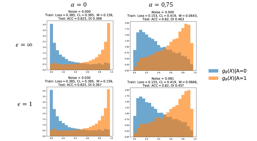
Figure 1: Histogram of $g_{\theta}(x)$ for the classification model minimizing (5), weight $\alpha\in\{0,0.75\}$ and privacy budget $\epsilon\in\{\infty,1\}$.

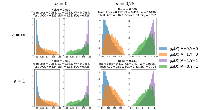
Figure 2: Histogram of $g_{\theta}(x)$ for the classification model minimizing (6), weight $\alpha\in\{0,0.75\}$ and privacy budget $\epsilon\in\{\infty,1\}$.

Fair representation learning. The aim is to privately learn fair encoder-decoder maps. To achieve this, we train an autoencoder privately, with $\theta=(\theta_{a},\theta_{b})$, encoder $\varphi_{\theta}=\varphi_{\theta_{a}}$, bi-dimensional latent space, and decoder $\psi_{\theta}=\psi_{\theta_{b}}$, minimizing a version of (5), where statistical parity penalization is imposed on the latent space, and $l(\psi_{\theta}(\varphi_{\theta}(x)))=\|\psi_{\theta}(\varphi_{\theta}(x))-x\|^{2}$. Figure 3 shows the results obtained, increasing values of $\alpha$ reduce the discrepancy between the conditional distributions in the latent space. In addition, Figures 3 and 4 show that privacy does not have a significative effect on the optimization.

Regression. In our generating mechanism, the label $Y\in\{0,1\}$ is defined as a set indicator function of a continuous response $Y^{C}\in[0,1]\times[0,1]$. We train a two-layer neural network privately with statistical parity penalization and $l(g_{\theta}(x),y)=\|g_{\theta}(x)-y\|^{2}$. See Appendix B.

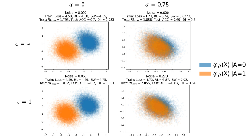
Figure 3: Encoded values $\varphi_{\theta}(x)$ for the autoencoder model minimizing (5), weight $\alpha\in\{0,0.75\}$, privacy budget $\epsilon\in\{\infty,1\}$.

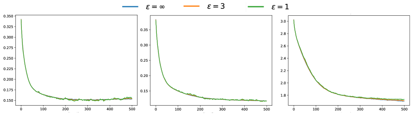
Figure 4: From left to right, training losses of Figures 1, 2 and 3 for $\alpha=0.75$ and different values of $\epsilon$.

8 Conclusion

In this work, we have provided a novel and practical method to ensure Differential Privacy for (sliced) Wasserstein gradients. By embedding DP guarantees into these gradients, we can preserve their statistical utility while ensuring that the training process does not inadvertently expose sensitive data. We tackle not only the constraint of statistical parity but also the Equality of Odds constraint to guarantee a fair accuracy for all. This synergy is crucial in fairness-sensitive high risk domains as denoted in the AI European Act (e.g., healthcare, criminal justice, access to public resources), where models must balance the dual imperatives of privacy preservation and equitable performance across subgroups. Our methodology is versatile and can is also useful to many other applications in Machine Learning such as representation learning or data generation, i.e., in all tasks where a Sliced Wasserstein metric is involved.

This work opens many research directions. Our results do not generalize to other Wasserstein losses, such as $W_{p}$. We prove in Appendix D that, in general, it is not possible to bound the sensitivity of the gradient of $W_{p}$, for general $p\geq 1$, by a factor that decreases approximately as $1/n$. Yet we believe that the generalization of our method to $W_{p}^{p}$ can be tackled and is worth of interest. A natural extension to the privacy of the computation of sliced Wasserstein barycenters is also left for future research.

Impact Statement

This paper presents work whose goal is to advance the field of Privacy-Preserving and Fair Machine Learning. This work is theoretical. There are many potential societal consequences of our work, none which we feel must be specifically highlighted here.

Appendix A Proofs

A.1 Proofs of Section 3

Proof of Proposition 3.1.

If we denote by $F$ and $G$ the distribution functions of $P_{\mathbf{U}}$ and $P_{\mathbf{V}}$, we know that

$$W_{2}^{2}(P_{\mathbf{U}},P_{\mathbf{V}}) =\int_{0}^{1}(F^{-1}(t)-G^{-1}(t))^{2}dt$$

$$=\int_{0}^{1}\Bigl{(}\sum_{i=1}^{n}U_{(i)}I\Bigl{(}\frac{i-1}{n}<t\leq\frac{i}{n}\Bigr{)}-\sum_{j=1}^{m}V_{(j)}I\Bigl{(}\frac{j-1}{m}<t\leq\frac{j}{n}\Bigr{)}\Bigr{)}^{2}dt$$

$$=\sum_{i=1}^{n}\sum_{j=1}^{m}(U_{(i)}-V_{(j)})^{2}\int_{0}^{1}I\Bigl{(}\frac{i-1}{n}<t\leq\frac{i}{n},\frac{j-1}{m}<t\leq\frac{j}{n}\Bigr{)}dt$$

$$=\sum_{i=1}^{n}\sum_{j=1}^{m}(U_{(i)}-V_{(j)})^{2}R_{i,j}$$

$$=\sum_{i=1}^{n}\sum_{j=1}^{m}(U_{(\sigma(i))}-V_{(\sigma(j))})^{2}R_{\sigma(i),\sigma(j)}$$

$$=\sum_{i=1}^{n}\sum_{j=1}^{m}(U_{i}-V_{j})^{2}R_{\sigma(i),\sigma(j)}\ ,$$

where the third equality follows from the fact that exactly one element in each sum is different from 0, and the fifth equality follows from reindexing the sum.∎

A.2 Proofs of Section 4

Proof of Theorem 4.1.

First of all, note that (b) follows immediately from (a) and the definition of the neighboring relation $\sim_{2}$ in $\mathcal{X}^{n}\times\mathcal{Z}^{m}$. Consider two neighboring datasets $\mathbf{X}\sim\mathbf{\tilde{X}}$ under the substitution relation. We can assume without loss of generality that the datasets differ on the first observation $\tilde{x}_{1}\neq x_{1}$. For ease of notation, denote $\mathbf{\tilde{X}}=\{\tilde{x}_{i}\}_{i=1}^{n}$, even though $\tilde{x}_{i}=x_{i}$ for $i\neq 1$. Along this proof, we will define $U_{i}:=g_{\theta}(x_{i})$ and $\tilde{U}_{i}:=g_{\theta}(\tilde{x}_{i})$ for each $i\in[n]$, and $V_{j}:=h_{\theta}(z_{j})$ for $j\in[m]$. Again, $U_{i}=\tilde{U}_{i}$ for every $i\neq 1$. Define now the rank permutations $\sigma,\tilde{\sigma}$ and $\tau$ such that

$$U_{i} =U_{(\sigma(i))}\ ,\quad\ i\in[n]\ ,$$

$$\tilde{U}_{i} =\tilde{U}_{(\tilde{\sigma}(i))}\ ,\quad\ i\in[n]\ ,$$

$$V_{j} =V_{(\tau(j))}\ ,\quad\ j\in[m]\ .$$

Denote $\mathbf{U}=(U_{1},\ldots,U_{n})$ and $\mathbf{V}=(V_{1},\ldots,V_{m})$. Corollary 3.2 ensures if we define $P_{\mathbf{U}}=g_{\theta}\#P_{\mathbf{X}}=\frac{1}{n}\sum_{i=1}^{n}\delta_{U_{i}}$ and $P_{\mathbf{V}}=h_{\theta}\#P_{\mathbf{Z}}=\frac{1}{m}\sum_{i=1}^{m}\delta_{V_{j}}$ , then

$$\nabla_{U,V}W_{2}^{2}(P_{\mathbf{U}},P_{\mathbf{V}})=\Biggl{(}\Bigl{(}2\sum_{j=1}^{m}R_{\sigma(i),\tau(j)}(U_{i}-V_{j})\Bigr{)}_{i\in[n]},\Bigl{(}2\sum_{i=1}^{n}R_{\sigma(i),\tau(j)}(V_{j}-U_{i})\Bigr{)}_{j\in[m]}\Biggr{)}\ \in\mathbb{R}^{n+m}\ .$$

Applying the chain rule, we obtain that

$$\nabla_{\theta}W_{2}^{2}(g_{\theta}\#P_{\mathbf{X}},h_{\theta}\#P_{\mathbf{Z}}) =2\sum_{i=1}^{n}\sum_{j=1}^{m}R_{\sigma(i),\tau(j)}(U_{i}-V_{j})\nabla_{\theta}g_{\theta}(x_{i})+2\sum_{j=1}^{m}\sum_{i=1}^{n}R_{\sigma(i),\tau(j)}(V_{j}-U_{i})\nabla_{\theta}h_{\theta}(z_{j})$$

Similarly, for the dataset $\mathbf{\tilde{X}}$ we get

$$\nabla_{\theta}W_{2}^{2}(g_{\theta}\#P_{\mathbf{\tilde{X}}},h_{\theta}\#P_{\mathbf{Z}}) =2\sum_{i=1}^{n}\sum_{j=1}^{m}R_{\tilde{\sigma}(i),\tau(j)}(\tilde{U}_{i}-V_{j})\nabla_{\theta}g_{\theta}(\tilde{x}_{i})+2\sum_{j=1}^{m}\sum_{i=1}^{n}R_{\tilde{\sigma}(i),\tau(j)}(V_{j}-\tilde{U}_{i})\nabla_{\theta}h_{\theta}(z_{j})$$

Therefore,

$$\|\nabla_{\theta}W_{2}^{2} (g_{\theta}\#P_{\mathbf{X}},h_{\theta}\#P_{\mathbf{Z}})-\nabla_{\theta}W_{2}^{2}(g_{\theta}\#P_{\mathbf{\tilde{X}}},h_{\theta}\#P_{\mathbf{Z}})\|_{2}\leq$$

$$\leq 2\ \Big{\|}\sum_{i=1}^{n}\sum_{j=1}^{m}R_{\sigma(i),\tau(j)}(U_{i}-V_{j})\nabla_{\theta}g_{\theta}(x_{i})-\sum_{i=1}^{n}\sum_{j=1}^{m}R_{\tilde{\sigma}(i),\tau(j)}(\tilde{U}_{i}-V_{j})\nabla_{\theta}g_{\theta}(\tilde{x}_{i})\Big{\|}_{2}$$ (9)

$$+2\ \Big{\|}\sum_{j=1}^{m}\sum_{i=1}^{n}R_{\sigma(i),\tau(j)}(V_{j}-U_{i})\nabla_{\theta}h_{\theta}(z_{j})-\sum_{j=1}^{m}\sum_{i=1}^{n}R_{\tilde{\sigma}(i),\tau(j)}(V_{j}-\tilde{U}_{i})\nabla_{\theta}h_{\theta}(z_{j})\Big{\|}_{2}$$ (10)

The term (10) is easier to bound, since the values inside $\nabla_{\theta}h_{\theta}(\cdot)$ coincide. First, note that

$$\sum_{j=1}^{m}R_{i,j}=\frac{1}{n}\ ,\ \forall\ i\in[n]\quad\textnormal{and}\quad\sum_{i=1}^{n}R_{i,j}=\frac{1}{m}\ ,\ \forall\ j\in[m]\ ,$$ (11)

The triangular inequality, the assumption $\|\nabla_{\theta}h_{\theta}(z)\|\leq L_{2}$ for every $z,\theta$ and the previous property allow us to derive the following inequalities

$$(\ref{eq:term2}) =2\ \Big{\|}\sum_{j=1}^{m}V_{j}\nabla_{\theta}h_{\theta}(z_{j})\Bigl{(}\sum_{i=1}^{n}R_{\sigma(i),\tau(j)}-\sum_{i=1}^{n}R_{\tilde{\sigma}(i),\tau(j)}\Bigr{)}-\sum_{j=1}^{m}\nabla_{\theta}h_{\theta}(z_{j})\Bigl{(}\sum_{i=1}^{n}U_{i}R_{\sigma(i),\tau(j)}-\sum_{i=1}^{n}\tilde{U}_{i}R_{\tilde{\sigma}(i),\tau(j)}\Bigr{)}\Big{\|}_{2}$$

$$\leq 2\sum_{j=1}^{m}\Bigl{\|}\nabla_{\theta}h_{\theta}(z_{j})\Bigl{(}\sum_{i=1}^{n}U_{i}R_{\sigma(i),\tau(j)}-\sum_{i=1}^{n}\tilde{U}_{i}R_{\tilde{\sigma}(i),\tau(j)}\Bigr{)}\Big{\|}_{2}$$

$$\leq 2L_{2}\sum_{j=1}^{m}\Bigl{|}\sum_{i=1}^{n}U_{i}R_{\sigma(i),\tau(j)}-\sum_{i=1}^{n}\tilde{U}_{i}R_{\tilde{\sigma}(i),\tau(j)}\Big{|}$$

$$=2L_{2}\sum_{j=1}^{m}\Bigl{|}\sum_{i=1}^{n}U_{(i)}R_{i,\tau(j)}-\sum_{i=1}^{n}\tilde{U}_{(i)}R_{i,\tau(j)}\Big{|}$$

$$=2L_{2}\sum_{j=1}^{m}\Bigl{|}\sum_{i=1}^{n}R_{i,\tau(j)}(U_{(i)}-\tilde{U}_{(i)})\Big{|}$$ (12)

where the last lines follows from $U_{i}=U_{(\sigma(i))}$, $\tilde{U}_{i}=\tilde{U}_{(\tilde{\sigma}(i))}$ and reindexing the sum. Since $U_{i}=\tilde{U}_{i}$ for every $i\neq 1$, we know that

• If $U_{1}\geq\tilde{U}_{1}$, then $U_{(i)}\geq\tilde{U}_{(i)}$ for every $i\in[n]$.

• If $U_{1}<\tilde{U}_{1}$, then $U_{(i)}\leq\tilde{U}_{(i)}$ for every $i\in[n]$.

This monotonicity property and the fact that $R_{i,j}\geq 0$ for every $i,j$ ensures that

$$(\ref{eq:last_line_ineq}) =2L_{2}\ \Bigl{|}\sum_{j=1}^{m}\sum_{i=1}^{n}R_{i,\tau(j)}(U_{(i)}-\tilde{U}_{(i)})\Big{|}$$

$$=2L_{2}\ \Bigl{|}\sum_{i=1}^{n}(U_{(i)}-\tilde{U}_{(i)})\sum_{j=1}^{m}R_{i,\tau(j)}\Big{|}$$

$$=\frac{2L_{2}}{n}\ \Bigl{|}\sum_{i=1}^{n}(U_{(i)}-\tilde{U}_{(i)})\Big{|}$$

$$=\frac{2L_{2}}{n}\Bigl{|}\sum_{i=1}^{n}(U_{i}-\tilde{U}_{i})\Big{|}$$

$$=\frac{2L_{2}}{n}\bigr{|}U_{1}-\tilde{U}_{1}\big{|}$$

$$\leq\frac{4L_{2}M}{n}$$

By the triangular inequality, the term (9) can be bounded as follows

$$(\ref{eq:term1}) \leq 2\ \Big{\|}\sum_{i=1}^{n}\nabla_{\theta}g_{\theta}(x_{i})U_{i}\sum_{j=1}^{m}R_{\sigma(i),\tau(j)}-\sum_{i=1}^{n}\nabla_{\theta}g_{\theta}(\tilde{x}_{i})\tilde{U}_{i}\sum_{j=1}^{m}R_{\tilde{\sigma}(i),\tau(j)}\Big{\|}_{2}$$ (13)

$$\quad+2\ \Big{\|}\nabla_{\theta}g_{\theta}(x_{1})\sum_{j=1}^{m}R_{\sigma(1),\tau(j)}V_{j}-\nabla_{\theta}g_{\theta}(\tilde{x}_{1})\sum_{j=1}^{m}R_{\tilde{\sigma}(1),\tau(j)}V_{j}\Big{\|}_{2}$$ (14)

$$\quad+2\ \Big{\|}\sum_{i=2}^{n}\nabla_{\theta}g_{\theta}(x_{i})\sum_{j=1}^{m}V_{j}(R_{\sigma(i),\tau(j)}-R_{\tilde{\sigma}(i),\tau(j)})\Big{\|}_{2}$$ (15)

We can bound independently each term in the decomposition,

$$(\ref{eq:decomp1}) =\frac{2}{n}\Big{\|}\sum_{i=1}^{n}\nabla_{\theta}g_{\theta}(x_{i})U_{i}-\nabla_{\theta}g_{\theta}(\tilde{x}_{i})\tilde{U}_{i}\Big{\|}_{2}$$

$$=\frac{2}{n}\Big{\|}\nabla_{\theta}g_{\theta}(x_{1})U_{1}-\nabla_{\theta}g_{\theta}(\tilde{x}_{1})\tilde{U}_{1}\Big{\|}_{2}$$

$$\leq\frac{2}{n}\Bigl{(}|U_{1}|\|\nabla_{\theta}g_{\theta}(x_{1})\|_{2}+|\tilde{U}_{1}|\|\nabla_{\theta}g_{\theta}(\tilde{x}_{1})\|_{2}\Bigr{)}$$

$$\leq\frac{4L_{1}M}{n}$$

$$(\ref{eq:decomp2}) \leq 2L_{1}M\Bigl{(}\sum_{j=1}^{m}R_{\sigma(1),\tau(j)}+\sum_{j=1}^{m}R_{\tilde{\sigma}(1),\tau(j)}\Bigr{)}$$

$$=\frac{4L_{1}M}{n}$$

$$(\ref{eq:decomp3}) \leq 2L_{1}\ \sum_{i=2}^{n}\Big{|}\sum_{j=1}^{m}V_{j}(R_{\sigma(i),\tau(j)}-R_{\tilde{\sigma}(i),\tau(j)})\Big{|}$$

$$=2L_{1}\ \sum_{i=2}^{n}\Big{|}\sum_{j=1}^{m}V_{(j)}(R_{\sigma(i),j)}-R_{\tilde{\sigma}(i),j})\Big{|}$$ (16)

The last equality is a simple consequence of $V_{j}=V_{(\tau(j))}$ and reindexing the sum. To bound the last expression, it is useful to see that all the terms $\sum_{j=1}^{m}V_{(j)}(R_{\sigma(i),j)}-R_{\tilde{\sigma}(i),j})$ have the same sign, for $i=2,\ldots,n$. This will follow from the relationship between the permutations $\sigma$ and $\tilde{\sigma}$. For instance, if $\tilde{\sigma}(1)<\sigma(1)$, it follows that

1. $\tilde{\sigma}(i)\geq\sigma(i)$ for every $i\geq 2$. Remember that $\sigma(i)$ denotes the position of $U_{i}$ in the ordered statistic $(U_{(1)},\ldots,U_{(n)})$, and $\tilde{\sigma}(i)$ denotes the position of $\tilde{U}_{i}$ in the ordered statistic $(\tilde{U}_{(1)},\ldots,\tilde{U}_{(n)}^{\prime})$. Recall also that $\tilde{U}_{i}=U_{i}$ for every $i\geq 2$. Therefore, $\tilde{\sigma}(1)<\sigma(1)$ implies that $\tilde{U}_{1}<U_{1}$, and

   • If $\sigma(i)<\tilde{\sigma}(1)$, then $\tilde{\sigma}(i)=\sigma(i)$.

   • If $\sigma(i)=\tilde{\sigma}(1)$, then $\tilde{\sigma}(i)=\sigma(i)$ if $U_{i}<\tilde{U}_{1}$, and $\tilde{\sigma}(i)=\sigma(i)+1$ if $U_{i}>\tilde{U}_{1}$.

   • If $\tilde{\sigma}(1)<\sigma(i)<\sigma(1)$, then $\tilde{\sigma}(i)=\sigma(i)+1$.

   • If $\sigma(i)>\sigma(1)$, then $\tilde{\sigma}(i)=\sigma(i)$.

2. $\sum_{j=1}^{m}V_{(j)}(R_{\sigma(i),j)}-R_{\tilde{\sigma}(i),j})\leq 0$ for every $i=2,\ldots,n$. If we denote by $G$ the empirical distribution function of $V_{1},\ldots,V_{m}$, then by definition of $R_{i,j}$,

   $$\sum_{j=1}^{m}V_{(j)} (R_{\sigma(i),j)}-R_{\tilde{\sigma}(i),j})=$$

   $$=\sum_{j=1}^{m}V_{(j)}\Biggl{(}\int_{\frac{\sigma(i)-1}{n}}^{\frac{\sigma(i)}{n}}I\Bigl{(}\frac{j-1}{m}<t\leq\frac{j}{m}\Bigr{)}dt-\int_{\frac{\tilde{\sigma}(i)-1}{n}}^{\frac{\tilde{\sigma}(i)}{n}}I\Bigl{(}\frac{j-1}{m}<t\leq\frac{j}{m}\Bigr{)}dt\Biggr{)}$$

   $$=\int_{\frac{\sigma(i)-1}{n}}^{\frac{\sigma(i)}{n}}\sum_{j=1}^{m}V_{(j)}I\Bigl{(}\frac{j-1}{m}<t\leq\frac{j}{m}\Bigr{)}dt-\int_{\frac{\tilde{\sigma}(i)-1}{n}}^{\frac{\tilde{\sigma}(i)}{n}}\sum_{j=1}^{m}V_{(j)}I\Bigl{(}\frac{j-1}{m}<t\leq\frac{j}{m}\Bigr{)}dt$$

   $$=\int_{\frac{\sigma(i)-1}{n}}^{\frac{\sigma(i)}{n}}G^{-1}(t)dt-\int_{\frac{\tilde{\sigma}(i)-1}{n}}^{\frac{\tilde{\sigma}(i)}{n}}G^{-1}(t)dt$$

   $$=\int_{\frac{\sigma(i)-1}{n}}^{\frac{\sigma(i)}{n}}G^{-1}(t)-G^{-1}\Bigl{(}t+\frac{\tilde{\sigma}(i)-\sigma(i)}{n}\Bigr{)}dt\leq 0$$

   for every $i=2,\ldots,n$, where the last bound is consequence of $(a)$ and the monotonicity of $G^{-1}$.

Similarly, if $\tilde{\sigma}(1)>\sigma(1)$, then $\tilde{\sigma}(i)\leq\sigma(i)$ for every $i\geq 2$, which implies $\sum_{j=1}^{m}V_{(j)}(R_{\sigma(i),j)}-R_{\tilde{\sigma}(i),j})\geq 0$. Finally, the case $\tilde{\sigma}(1)=\sigma(1)$ is trivial, since this implies $\tilde{\sigma}=\sigma$. Therefore, in any of the cases, the sign property implies that

$$(\ref{eq:last_inequality_2}) =2L_{1}\ \Big{|}\sum_{i=2}^{n}\sum_{j=1}^{m}V_{(j)}(R_{\sigma(i),j)}-R_{\tilde{\sigma}(i),j})\Big{|}$$

$$=2L_{1}\ \Big{|}\sum_{j=1}^{m}V_{(j)}\sum_{i=2}^{n}(R_{\sigma(i),j)}-R_{\tilde{\sigma}(i),j})\Big{|}$$

$$=2L_{1}\ \Big{|}\sum_{j=1}^{m}V_{(j)}\sum_{i=1}^{n}(R_{\sigma(i),j)}-R_{\tilde{\sigma}(i),j})-\sum_{j=1}^{m}V_{(j)}(R_{\sigma(1),j)}-R_{\tilde{\sigma}(1),j})\Big{|}$$

$$=2L_{1}\ \Big{|}\sum_{j=1}^{m}V_{(j)}(R_{\sigma(1),j)}-R_{\tilde{\sigma}(1),j})\Big{|}$$

$$\leq 2L_{1}M\Bigl{(}\sum_{j=1}^{m}R_{\sigma(1),\tau(j)}+\sum_{j=1}^{m}R_{\tilde{\sigma}(1),\tau(j)}\Bigr{)}$$

$$=\frac{4L_{1}M}{n}$$

Putting everything together, we can conclude that,

$$\|\nabla_{\theta}W_{2}^{2} (g_{\theta}\#P_{\mathbf{X}},h_{\theta}\#P_{\mathbf{Z}})-\nabla_{\theta}W_{2}^{2}(g_{\theta}\#P_{\mathbf{\tilde{X}}},h_{\theta}\#P_{\mathbf{Z}})\|_{2}\leq\frac{12L_{1}M}{n}+\frac{4L_{2}M}{n}\ .$$

∎

A.3 Extension to the sliced Wasserstein distance

As pointed out in Remark 4.2, the results of this paper can be extended to higher dimensions by considering the sliced Wasserstein distance. Assume that $g_{\theta}(x),h_{\theta}(x)\in\mathbb{R}^{d}$. Following the notation of Section 4, we are interested now in bounding the sensitivity of the gradient of the (squared) sliced Wasserstein distance between the distributions $g_{\theta}\#P_{\mathbf{X}}$ and $h_{\theta}\#P_{\mathbf{Z}}$ in $\mathbb{R}^{d}$, defined as

$${SW}_{2}^{2}( g_{\theta}\#P_{\mathbf{X}},h_{\theta}\#P_{\mathbf{Z}})=\int_{\mathbb{S}^{d-1}}W_{2}^{2}\Bigl{(}\operatorname{Pr}_{\vartheta}\#(g_{\theta}\#P_{\mathbf{X}}),\operatorname{Pr}_{\vartheta}\#(h_{\theta}\#P_{\mathbf{Z}})\Bigr{)}d\mu(\vartheta)\ ,$$

where $\mu$ represents the uniform measure on $\mathbb{S}^{d-1}$, the unit sphere of $\mathbb{R}^{d}$. From a practical standpoint, we are mainly interested in the study of the gradient of its Monte-Carlo approximation given by $k$ i.i.d. random directions $\vartheta_{1},\ldots,\vartheta_{k}\in\mathbb{S}^{d-1}$,

$${SW}_{2,k}^{2}( g_{\theta}\#P_{\mathbf{X}},h_{\theta}\#P_{\mathbf{Z}})=\frac{1}{k}\sum_{l=1}^{k}W_{2}^{2}\Bigl{(}\operatorname{Pr}_{\vartheta_{l}}\#(g_{\theta}\#P_{\mathbf{X}}),\operatorname{Pr}_{\vartheta_{l}}\#(h_{\theta}\#P_{\mathbf{Z}})\Bigr{)}\ .$$

As in the proof of Theorem 4.1, it suffices to bound the sensitivity of the gradient with respect to the substitution neighboring relation $\mathbf{X}\sim_{1}\mathbf{\tilde{X}}$. If we define $\Phi(\mathbf{X})=\nabla_{\theta}{SW}_{2}^{2}(g_{\theta}\#P_{\mathbf{X}},h_{\theta}\#P_{\mathbf{Z}})$ and $\Phi_{\vartheta}(\mathbf{X})=\nabla_{\theta}W_{2}^{2}(\operatorname{Pr}_{\vartheta}\#(g_{\theta}\#P_{\mathbf{X}}),\operatorname{Pr}_{\vartheta}\#(h_{\theta}\#P_{\mathbf{Z}}))$, by the chain rule and the same reasoning as in the proof of Theorem 1 in (Bonneel et al., 2015), we know that under suitable smoothness assumptions, in the set of non-repeated points $\Gamma=\{\theta:g_{\theta}(x_{i})\neq g_{\theta}(x_{j}),h_{\theta}(z_{i})\neq h_{\theta}(z_{j})\textnormal{ for }i\neq j\}$,

$$\Phi(\mathbf{X}) =\int_{\mathbb{S}^{d-1}}\Phi_{\vartheta}(\mathbf{X})d\mu(\vartheta)$$

As in Section 3, we can define the gradient $\Phi(\mathbf{X})$ by this expression, even outside the set of differentiability points $\Gamma$, and provide privacy guarantees for every point. Similarly, if we consider the Monte-Carlo approximation of the gradient $\Phi(\mathbf{X})=\nabla_{\theta}{SW}_{2,k}^{2}(g_{\theta}\#P_{\mathbf{X}},h_{\theta}\#P_{\mathbf{Z}})$, it follows that $\Phi(\mathbf{X})=\frac{1}{k}\sum_{l=1}^{k}\Phi_{\vartheta}(\mathbf{X})$. In any case, we can conclude that

$$\Delta\Phi=\sup_{\mathbf{X}\sim\mathbf{\tilde{X}}}\|\Phi(\mathbf{X})-\Phi(\mathbf{\tilde{X}})\|_{2}\leq\sup_{\vartheta\in\mathbb{S}^{d-1}}\Delta\Phi_{\vartheta}$$

The sensitivity of $\Phi_{\vartheta}$ can be controlled with the one-dimensional results in Section 4. Note that if we define $g_{\theta}^{\vartheta}(x)=\vartheta^{T}g_{\theta}(x)$ and $h_{\theta}^{\vartheta}(x)=\vartheta^{T}h_{\theta}(z)$, then $\Phi_{\vartheta}(\mathbf{X})=\nabla_{\theta}W_{2}^{2}(g_{\theta}^{\vartheta}\#P_{\mathbf{X}},h_{\theta}^{\vartheta}\#P_{\mathbf{Z}})$, and we can conclude

$$\Delta\Phi_{\vartheta}\leq\frac{12L_{1}M}{n}+\frac{4L_{2}M}{n}$$

provided that:

1. $|g_{\theta}^{\vartheta}(x)|=|\vartheta^{T}g_{\theta}(x)|\leq M$, $|h_{\theta}^{\vartheta}(x)|=|\vartheta^{T}h_{\theta}(z)|\leq M$ .

2. $\|\nabla_{\theta}g_{\theta}^{\vartheta}(x)\|_{2}=\|\vartheta^{T}\mathcal{J}_{\theta}g_{\theta}(x)\|_{2}\leq L_{1}$, $\|\vartheta^{T}\mathcal{J}_{\eta}h_{\theta}(z)\|_{2}\leq L_{2}$.

In particular, both inequalities are verified uniformly in $\vartheta$ if we impose the following, more natural conditions:

1. $\|g_{\theta}^{\vartheta}(x)\|_{2}\leq M$, $\|h_{\theta}(z)\|_{2}\leq M$

2. $\|\mathcal{J}_{\theta}g_{\theta}(x)\|_{2}=\sup_{\|\eta\|_{2}=1}\|J_{\theta}g_{\theta}(x)\eta\|_{2}\leq L_{1}$, $\|\mathcal{J}_{\theta}h_{\theta}(z)\|_{2}=\sup_{\|\eta\|_{2}=1}\|J_{\theta}h_{\theta}(z)\eta\|_{2}\leq L_{2}$.

The second assumption implies that for every $\vartheta\in\mathbb{S}^{d-1}$ and $x$,

$$\|\vartheta^{T}\mathcal{J}_{\theta}g_{\theta}(v_{j})\|_{2} =\vartheta^{T}\mathcal{J}_{\theta}g_{\theta}(x)\frac{\vartheta^{T}\mathcal{J}_{\theta}g_{\theta}(x)}{\|\vartheta^{T}\mathcal{J}_{\theta}g_{\theta}(x)\|_{2}}$$

$$\leq\|\vartheta\|_{2}\Big{\|}J_{\theta}g_{\theta}(x)\frac{\vartheta^{T}\mathcal{J}_{\theta}g_{\theta}(x)}{\|\vartheta^{T}\mathcal{J}_{\theta}g_{\theta}(x)\|_{2}}\Big{\|}_{2}$$

$$\leq L_{1}\;,$$

and similarly for $h_{\theta}$. As in the one dimensional setting, the second assumption is verified if $g_{\theta}$ and $h_{\theta}$ are $L_{1}$-Lipschitz and $L_{2}$-Lipschitz with respect to $\theta$. To see this, note that if $\|\eta\|_{2}=1$, by the Lipschitz condition,

$$\|\mathcal{J}_{\theta}g_{\theta}(x)\eta\|_{2} =\Big{\|}\lim_{t\rightarrow 0}\frac{g_{\theta+t\eta}(x)-g_{\theta}(x)}{t}\Big{\|}\leq L_{1}\|\eta\|_{2}=L_{1}$$

Therefore, Theorem 4.1 can be extended to the multidimensional setting with the sliced Wasserstein distance as follows:

Theorem A.1.

With all the previous notation, assume that there exists constants $M,L_{1},L_{2}\geq 0$ such that for each $\theta\in\Theta$, $x\in\mathcal{X}$ and $z\in\mathcal{Z}$,

1. $\|g_{\theta}(x)\|\leq M$, $\|h_{\theta}(z)\|_{2}\leq M$ .

2. $\|\mathcal{J}_{\theta}g_{\theta}(x)\|_{2}=\sup_{\|\eta\|_{2}=1}\|J_{\theta}g_{\theta}(x)\eta\|_{2}\leq L_{1}$, $\|\mathcal{J}_{\theta}h_{\theta}(z)\|_{2}=\sup_{\|\eta\|_{2}=1}\|J_{\theta}h_{\theta}(z)\eta\|_{2}\leq L_{2}$.

Then,

• Under neighboring relation $\sim_{1}$ in $\mathcal{D}=\mathcal{X}^{n}$, if we define $\Phi_{\theta}(\mathbf{X})$ as $\nabla_{\theta}SW_{2}^{2}(g_{\theta}\#P_{\mathbf{X}},h_{\theta}\#P_{\mathbf{Z}})$ or its Monte-Carlo approximation $\nabla_{\theta}SW_{2,k}^{2}(g_{\theta}\#P_{\mathbf{X}},h_{\theta}\#P_{\mathbf{Z}})$ then

  $$\Delta\Phi_{\theta}\leq 4M\frac{3L_{1}+L_{2}}{n}\ .$$

• Under neighboring relation $\sim_{2}$ in $\mathcal{D}=\mathcal{X}^{n}\times\mathcal{Z}^{m}$, if we define $\Psi_{\theta}(\mathbf{X},\mathbf{Z})$ as $\nabla_{\theta}SW_{2}^{2}(g_{\theta}\#P_{\mathbf{X}},h_{\theta}\#P_{\mathbf{Z}})$ or its Monte-Carlo approximation $\nabla_{\theta}SW_{2,k}^{2}(g_{\theta}\#P_{\mathbf{X}},h_{\theta}\#P_{\mathbf{Z}})$, then

  $$\Delta\Psi_{\theta}\leq 4M\max\Bigl{\{}\frac{3L_{1}+L_{2}}{n},\frac{L_{1}+3L_{2}}{m}\Bigr{\}}\ .$$

Remark A.2.

From a computational point of view, if we want to define a clipped approximation $\mathcal{J}^{L_{1}}_{\theta}g_{\theta}(x_{i})$ of $\mathcal{J}_{\theta}g_{\theta}(x_{i})$ that verifies Assumption 2 in Theorem A.1, this might be done by clipping the eigenvalues of the singular value decomposition of $\mathcal{J}_{\theta}g_{\theta}(x_{i})$. This should be done at each step, for each $x_{i}$ in the batch. To simplify the computation and enable easy parallelization, we have adopted a suboptimal, naive alternative approach. If $g_{\theta}=(g_{\theta}^{1},\ldots,g_{\theta}^{d})$, and we define

$$\mathcal{J}^{L_{1}}_{\theta}g_{\theta}(x_{i})=\left(\begin{array}[]{c}\operatorname{clip}_{\frac{L_{1}}{\sqrt{d}}}(\nabla_{\theta}g_{\theta}^{1})\\ \vdots\\ \operatorname{clip}_{\frac{L_{1}}{\sqrt{d}}}(\nabla_{\theta}g_{\theta}^{d})\end{array}\right)\ ,$$

then it is straightforward to see that $\|\mathcal{J}^{L_{1}}_{\theta}g_{\theta}(x)\|_{2}=\sup_{\|\eta\|_{2}=1}\|J^{L_{1}}_{\theta}g_{\theta}(x)\eta\|_{2}\leq L_{1}$.

A.4 Other Proofs

Proof of Lemma 5.1.

See the proof of Theorem 29 in (Steinke, 2022) which gives the result up to a minor adaptation. The term $\max\left({\frac{n_{1}^{\prime}}{n_{1}},\dots,\frac{n_{k}^{\prime}}{n_{k}}}\right)$ indeed comes from considering the worst case analysis depending on which category the differing point is in. ∎

Proof of Theorem 6.1.

Formally, with the notation of Definition 2.1, define for the first part $\mathcal{D}=\mathcal{D}_{0}^{n_{0}}\times\mathcal{D}_{1}^{n_{1}}$, where $\mathcal{D}_{j}=\mathcal{X}\times\mathcal{Y}\times\{j\}$ in the supervised case, and $\mathcal{D}_{j}=\mathcal{X}\times\{j\}$ in the unsupervised case, for $j=0,1$. Applying Theorem A.1 with $g_{\theta}=h_{\theta}$, we can bound the sensitivity of $\nabla_{\theta}\mathscr{L}^{SP}_{\alpha}(g_{\theta})$ by (7).

For the second part, consider $\mathcal{D}=\prod_{j,k}\mathcal{D}_{j,k}^{n_{j,k}}$, where $\mathcal{D}_{j,k}=\mathcal{X}\times\{j\}\times\{k\}$, for $j\in\{0,1\},k\in\{0,\ldots,R-1\}$. Under the relation $\sim_{2R}$, given two neighboring datasets, all the terms except one are the same in the sum in (5), and similarly for the gradient expression. More precisely, under the assumptions of the theorem, with the notation adopted in Section 6,

$$\sup_{\mathbf{D}\sim_{2R}\mathbf{\tilde{D}}}\Big{\|}\frac{1}{R}\sum_{k=1}^{K}\nabla_{\theta}{SW}_{2}^{2}\Bigl{(}g_{\theta}\#P_{\mathbf{X}_{0,k}},g_{\theta}\#P_{\mathbf{X}_{1,k}}\Bigr{)}-\frac{1}{R}\sum_{k=1}^{K}\nabla_{\theta}{SW}_{2}^{2}\Bigl{(}g_{\theta}\#P_{\mathbf{\tilde{X}}_{0,k}},g_{\theta}\#P_{\mathbf{\tilde{X}}_{1,k}}\Bigr{)}\Big{\|}_{2}$$

$$\leq\frac{1}{R}\sup_{\mathbf{D}\sim_{2R}\mathbf{\tilde{D}}}\sum_{k=1}^{K}\Big{\|}\nabla_{\theta}{SW}_{2}^{2}\Bigl{(}g_{\theta}\#P_{\mathbf{X}_{0,k}},g_{\theta}\#P_{\mathbf{X}_{1,k}}\Bigr{)}-\nabla_{\theta}{SW}_{2}^{2}\Bigl{(}g_{\theta}\#P_{\mathbf{\tilde{X}}_{0,k}},g_{\theta}\#P_{\mathbf{\tilde{X}}_{1,k}}\Bigr{)}\Big{\|}_{2}$$

$$\leq\frac{1}{R}\max_{k=0,\ldots,R-1}\sup_{(\mathbf{X}_{0,k},\mathbf{X}_{1,k})\sim_{2}(\mathbf{\tilde{X}}_{0,k},\mathbf{\tilde{X}}_{1,k})}\Big{\|}\nabla_{\theta}{SW}_{2}^{2}\Bigl{(}g_{\theta}\#P_{\mathbf{X}_{0,k}},g_{\theta}\#P_{\mathbf{X}_{1,k}}\Bigr{)}-\nabla_{\theta}{SW}_{2}^{2}\Bigl{(}g_{\theta}\#P_{\mathbf{\tilde{X}}_{0,k}},g_{\theta}\#P_{\mathbf{\tilde{X}}_{1,k}}\Bigr{)}\Big{\|}_{2}$$

$$\leq\frac{1}{R}\max_{k=0\ldots,R-1}\frac{16ML}{\min\{n_{0,k},n_{1,k}\}}=\frac{1}{R}\frac{16ML}{\min_{j,k}\{n_{j,k}\}}$$

which implies (8). ∎

Appendix B Additional details on the fairness experiments

In order to demonstrate the versatility of our methodology for imposing fairness in different scenarios, we use an illustrative model to simulate bias in algorithmic decision-making. Note that we do not provide comparisons with other application-specific methodologies, as our approach is highly general and does not include the statistical, convergence, or fairness guarantees that may be described by other methods, see (Xu et al., 2019; Jagielski et al., 2019; Ding et al., 2020; Lowy et al., 2022; Yaghini et al., 2023; Ghoukasian & Asoodeh, 2024) for the fair and private classification problem, or (Xian et al., 2024) for fair and private one-dimensional regression. Yet we provide, to our knowledge, the first method to handle novel problems such as multidimensional fair and private regression, or fair and private representation learning.

We consider $\mathbf{D}=\{(x_{i},a_{i},y_{i})\}_{i=1}^{n}$ i.i.d. samples with the same distribution as $(X,A,Y^{C},Y)$, where $X$ denotes the features, $A$ is the sensitive variable, $Y^{C}=(Y^{C}_{1},Y^{C}_{2})$ is a continuous response variable and $Y$ is a discrete version of $Y^{C}$, related by

1. $Y^{C}\sim U([0,1]\times[0,1])$

2. $Y=I\Bigl{(}Y^{C}_{2}>1-Y^{C}_{1}\Bigr{)}$

3. $A=BY+(1-B)(1-Y)$, where $B$ is a Bernoulli variable of parameter $p$ independent of Y.

4. $X_{core}=[\underbrace{Y^{C},\ldots,Y^{C}}_{d_{core}/2\ times}]+N\Bigl{(}0,\sigma^{2}_{core}\ I_{d_{core}}\Bigr{)}$, $\quad X_{spurious}=[\underbrace{A,\ldots,A}_{d_{sp}\ times}]+N\Bigl{(}0,\sigma^{2}_{sp}\ I_{d_{sp}}\Bigr{)}$

5. $X=[X_{core},X_{sp}]$

Therefore, this generated data consists in a response variable $Y_{C}$, which is correlated with the sensitive attribute $A$. The features $X$ can be divided into two parts: a first part $X_{core}$ which is a noisy transformation of $Y_{C}$, and a second spurious part $X_{sp}$ which is a noisy version of $A$. If $p$ is close to 1, most of the cases verify $A=Y$ and therefore, the decision of the algorithm relies highly on the sensitive variable $A$. Bias in the algorithmic decision is created when the sensitive variable $A$ is not aligned with the decision. When $Y\neq A$, the learning task is more complicated since while $X_{core}$ is correlated with $Y$, the spurious part pushes towards the bad decision. This setting reproduces the characteristics of some of the main biases present in many data sets, for instance, (Becker & Kohavi, 1996) or (Hofmann, 1994) in supervised learning. We will explore this problem in different situations, and we will show how penalized models with our Wasserstein losses can help to alleviate the unfairness of these models, according to different notions, while preserving privacy guarantees. In all our experiments we will consider $n=30000$, $p=0.7$, $d_{core}=d_{sp}=8$, $\sigma^{2}_{core}=1/5$, $\sigma^{2}_{sp}=2/5$.

All models are trained with DP-SGD as explained in Section 5, with clipping constant $C>0$ for the individual gradients in (4), as usual in DP-SGD, and inner clipping constants $M,L>0$ for the Wasserstein gradient approximation (3) or its sliced version. In the latter case, all the experiments use the naive clipping procedure explained in Remark A.2. Theorem 6.1 and the procedure described in Section 5, enable us to compute the privacy budget obtained after $T$ iterations of DP-SGD. In particular, in all the experiments, we fix the number of iterations $T$ and the value of $\delta$, and compute the required noise to obtain $(\epsilon,\delta)$-DP after $T$ iterations, for different values of the privacy budget $\epsilon$ and the weight $\alpha\in[0,1]$ in the penalized loss functions (5) and (6). Batch sizes are $n^{\prime}_{j}\approx n_{j}/5$ when minimizing (5), and $n^{\prime}_{j,k}\approx n_{j,k}/5$ when minimizing (6), where the approximation is related to internal parallelization of the gradient computations in the code.

Following the notation of the main text, denote $\mathbf{X}_{j}=(x_{i}:a_{i}=j)$, $n_{j}=\textnormal{length}(\mathbf{X}_{j})$ for $j=0,1$, and $\mathbf{X}_{j,k}=(x_{i}:a_{i}=j,y_{i}=k)$, $n_{j,k}=\textnormal{length}(\mathbf{X}_{j,k})$ for $j,k\in\{0,1\}$. Given our data generation procedure, we know that $\mathbb{E}(n_{j})=n/2$, $\mathbb{E}(n_{j,j})=pn/2$ and $\mathbb{E}(n_{j,1-j})=(1-p)n/2$ for $j\in\{0,1\}$.

B.1 Classification

First, we consider the problem of predicting the label $Y$ as a function of $X$. Our decision rule is based on logistic regression, where the function $g_{\theta}$ maps each $x_{i}$ to the predicted probability $g_{\theta}(x_{i})\in(0,1)$. The classification rule is given by $G_{\theta}(x)=I(g_{\theta}(x)>1/2)$. $g_{\theta}$ is defined as a neural network with one layer and a sigmoid activation function, and it is trained with DP-SGD and a binary cross-entropy loss function, denoted by $\ell_{bce}$. We have analyzed fairness using two of the most common notions.

• Statistical parity: Statistical parity corresponds to the situation where the algorithmic decision does not depend on the sensitive variable. It is usually measured by the Disparate Impact, defined as

  $$DI(G_{\theta})=\frac{\mathbb{P}(G_{\theta}(X)=1|A=0)}{\mathbb{P}(G_{\theta}(X)=1|A=1)}\ .$$ (17)

  Enforcing statistical parity by enforcing independence between $G_{\theta}(X)$ and $A$ often produces unstable solutions as discussed in (Krco et al., 2025) or (Barrainkua et al., 2024), hence many authors propose to mitigate not only the mean but the whole distribution of the predicted probabilities $g_{\theta}(X)\in(0,1)$ as in (Risser et al., 2022), (Gouic et al., 2020) or (Chzhen et al., 2020). Statistical parity is thus satisfied if $\mathcal{L}(g_{\theta}(X)|A=0)=\mathcal{L}(g_{\theta}(X)|A=1)$. In our discrete setting, statistical parity can be favored by minimizing

  $$\mathscr{L}^{SP}_{\alpha}(g_{\theta})=(1-\alpha)\frac{1}{n}\sum_{i=1}^{n}\ell_{bce}(g_{\theta}(x_{i}),y_{i})+\alpha W_{2}^{2}\Bigl{(}g_{\theta}\#P_{\mathbf{X}_{0}},g_{\theta}\#P_{\mathbf{X}_{1}}\Bigr{)}$$ (18)

  In Figure 5 we present the results obtained for different values of the weight $\alpha$ and the privacy budget $\epsilon$, when we fix $\delta=0.1/n$, number of iterations $T=500$, clipping constants $C=5$, $M=L=1$ and learning rate $=0.05$. For every pair of $\alpha$ and $\epsilon$, we plot the histograms of the distribution of the predicted probabilities $g_{\theta}(X)|A=0$ and $g_{\theta}(X)|A=1$. Above each graph, we can see the noise required to achieve the privacy budget in the fixed number of iterations, the weighted training loss value obtained and the specific values of each term in the loss, and the accuracy and disparate impact of $G_{\theta}$ on test data. Two main conclusions can be drawn from Figure 5. First, it confirms that the Wasserstein penalization approach mitigates the unfair biases present in the data set. We can see that, for increasing values of $\alpha$, the histograms of the scores conditioned by the value of the sensitive variable get closer, leading to a progressive reduction of biases, as seen in the decreasing values of the disparate impact, albeit at the expense of accuracy, as expected. The second important conclusion is that adding privacy does not significantly alter the results of the optimization. For different privacy budgets $\epsilon$, both the histogram and the computed measures do not change much across the rows. Moreover, Figure 6 shows the training loss curve of the optimization for each value of $\alpha$ considered when $\epsilon$ varies. Low values of $\epsilon$ lead to noisy versions of the loss curve, but very close to the non-private version.

  

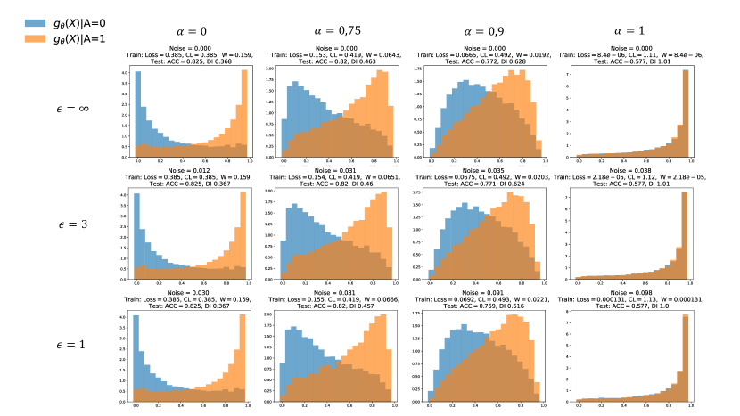
  Figure 5: Histogram of the predicted probabilities $g_{\theta}(X)$ of the model conditioned by the sensitive attribute $A=0,1$ in the training set. $\theta$ is the parameter obtained after 500 iterations of DP-SGD minimizing 18 for the different values of $\alpha$ (columns), with different privacy budgets $\epsilon$ (rows) for $\delta=0.1/n$ fixed. The parameters of the optimization are the learning rate $=0.05$, clipping values $C=5,\ M=1,\ L=1$, batch sizes $n_{0}^{\prime}\approx n_{0}/5,n_{1}^{\prime}\approx n_{1}/5$. Above each graph we indicate the noise added at each step of DP-SGD to obtain the desired privacy level, the value of the loss 18 in the training procedure, together with the individual value of the classification loss (CL) and the distributional Wasserstein loss (W). Last line includes accuracy (ACC) and disparate impact (DI) of the classification rule $G_{\theta}$ computed with independent test data set.

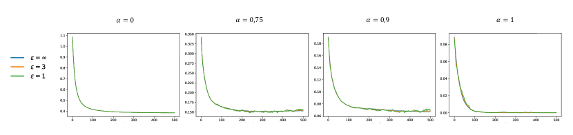
Figure 6: Training loss curve for the experiment of Figure 5. Each graph represents the training loss (18) for a fixed value of $\alpha$ along the iterations of DP-SGD, for the different privacy budgets of the experiments.

• Equality of odds: Beyond guaranteeing the same decision for all, which is not suitable in some cases where the sensitive variable impacts the decision, bias mitigation may require that the model performs with the same accuracy for all groups, often referred to as equality of odds. Usual measures of this bias for a classification rule $G_{\theta}$ are computed using the two following indexes:

  $$EO_{1}(G_{\theta}) =\frac{\mathbb{P}(G_{\theta}(X)=1|A=0,Y=1)}{\mathbb{P}(G_{\theta}(X)=1|A=1,Y=1)}\ .$$ (19)

  $$EO_{0}(G_{\theta}) =\frac{\mathbb{P}(G_{\theta}(X)=1|A=0,Y=0)}{\mathbb{P}(G_{\theta}(X)=1|A=1,Y=0)}\ .$$ (20)

  With the same ideas as before, Equality of Odds bias mitigation can be enforced for the distribution of the predicted probabilities $g_{\theta}$ by enforcing that $\mathcal{L}(g_{\theta}(X)|A=0,Y=j)=\mathcal{L}(g_{\theta}(X)|A=1,Y=j)$ for $j=0,1$. For this, we train the model with the penalized loss

  $$\mathscr{L}^{EOO}_{\alpha}(g_{\theta})=(1-\alpha)\frac{1}{n}\sum_{i=1}^{n}\ell_{bce}(g_{\theta}(x_{i}),y_{i})+\frac{\alpha}{2}W_{2}^{2}\Bigl{(}g_{\theta}\#P_{\mathbf{X}_{0,0}},g_{\theta}\#P_{\mathbf{X}_{1,0}}\Bigr{)}+\frac{\alpha}{2}W_{2}^{2}\Bigl{(}g_{\theta}\#P_{\mathbf{X}_{0,1}},g_{\theta}\#P_{\mathbf{X}_{1,1}}\Bigr{)}\ .$$ (21)

  Figure 7 shows the results of training the model minimizing 6 for different values of $\alpha$ and the privacy budget $\epsilon$, with fixed $\delta=0.1/n$, number of iterations $T=500$, clipping constants $C=5$, $M=L=1$ and learning rate $=0.05$. The histogram of the distribution of the predicted probabilities, $g_{\theta}(X)|A=1,Y=j$ versus $g_{\theta}(X)|A=0,Y=j$, illustrates the model’s capability to minimize discrepancies between the distributions as $\alpha$ increases, as shown by the values of $EO_{0},EO_{1}$. From Figure 7, we can also observe that private training has minimal impact on the model’s fit across all values of $\alpha$. Similarly, it does not significantly affect the learning loss curve during optimization, as shown in Figure 8.

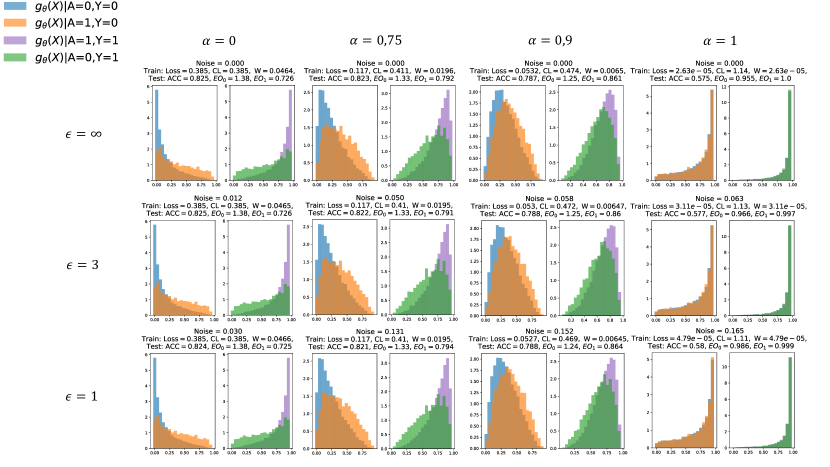
Figure 7: Histogram of the predicted probabilities $g_{\theta}(X)$ of the model conditioned by the sensitive attribute $A=0,1$ and the label $Y=0,1$ in the training set. $\theta$ is the parameter obtained after 500 iterations of DP-SGD minimizing (21) for the different values of $\alpha$ (columns), with different privacy budgets $\epsilon$ (rows) for $\delta=0.1/n$ fixed. The parameters of the optimization are the learning rate $=0.05$, clipping values $C=5,\ M=1,\ L=1$, batch sizes $n_{0}^{\prime}\approx n_{0}/5,n_{1}^{\prime}\approx n_{1}/5$. Above each graph we indicate the noise added at each step of DP-SGD to obtain the desired privacy level, the value of the loss (21) in the training procedure, together with the individual value of the classification loss (L) and the Wasserstein loss (W). Last line includes accuracy, $EO_{0}$ and $EO_{1}$ indexes computed with test data set.

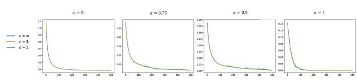
Figure 8: Training loss curve for the experiment of Figure 7. Each graph represents the training loss (21) for a fixed value of $\alpha$ along the iterations of DP-SGD, for the different privacy budgets of the experiments.

B.2 Regression

In our generating mechanism, the label $Y\in\{0,1\}$ is defined as a set indicator function of a continuous response $Y^{C}\in[0,1]\times[0,1]$. From the data-generating process, it is easy to derive the distribution of $Y_{C}$ conditioned by the sensitive attribute. If $T_{0}$ denotes the triangle with vertices $(0,0),(0,1),(1,0)$ and $T_{1}$ the triangles with vertices $(0,1),(1,1),(1,0)$, the we know that $Y^{C}|A=j$ follows a mixture of the uniform distributions on $T_{0}$ and $T_{1}$, with weight $p$ in $T_{0}$ and $(1-p)$ in $T_{1}$ if $A=0$, and vice versa if $A=1$. The aim of this experiment is to perform private and bi-dimensional fair regression over $Y_{C}$, which has never been considered before in the literature. To simplify our clipping bounds, we have centered our data to obtain a distribution in $[-1/2,1/2]\times[-1/2,1/2]$, and we have trained a two-layer neural network with hidden dimension 64, sigmoid activation function in the last layer, with the output centered by subtracting $(1/2,1/2)$, and minimizing the loss

$$\mathscr{L}^{SP}_{\alpha}(g_{\theta})=(1-\alpha)\frac{1}{n}\sum_{i=1}^{n}\|g_{\theta}(x_{i})-y_{i}^{C}\|_{2}^{2}+\alpha SW_{2}^{2}\Bigl{(}g_{\theta}\#P_{\mathbf{X}_{0}},g_{\theta}\#P_{\mathbf{X}_{1}}\Bigr{)}$$ (22)

Figure 9 shows the results of this experiment for different values of $\alpha$ and the privacy budget $\epsilon$, with fixed $\delta=0.1/n$, number of iterations $T=1000$, clipping constants $C=10$, $M=1/\sqrt{2}$, $L=\sqrt{2}$, learning rate $=0.05$ and number of projections in the Monte Carlo approximation $=50$. From the visual inspection of the plots, we can appreciate that our statistical parity penalization helps to reduce the differences between the distributions of the predicted values. To aid visual inspection, we provide the values of the number of points over the diagonal for each class $A=0$ and $A=1$. If $g_{\theta}(x)=(g^{1}_{\theta}(x),g^{2}_{\theta}(x))$

$$OD_{0}=\frac{\#\{X:g^{2}_{\theta}(X)>-g^{1}_{\theta}(X),A=0\}}{n_{0}}$$

$$OD_{1}=\frac{\#\{X:g^{2}_{\theta}(X)>-g^{1}_{\theta}(X),A=1\}}{n_{1}}$$

Finally, Figure 10 shows the convergence of the loss curve for the different values of $\alpha$ and $\epsilon$. As in the previous examples, the private loss curves are simply noisy versions of the non-private ones.

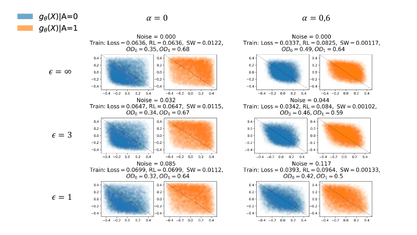
Figure 9: Plot of $g_{\theta}(X)$ conditioned by the sensitive attribute $A=0,1$ in the training set. $\theta$ is the parameter obtained after 1000 iterations of DP-SGD minimizing (22) for the different values of $\alpha$ (columns), with different privacy budgets $\epsilon$ (rows) for $\delta=0.1/n$ fixed. The parameters of the optimization are the learning rate $=0.05$, clipping values $C=10,\ M=1/\sqrt{2},\ L=\sqrt{2}$, batch sizes $n_{0}^{\prime}\approx n_{0}/5,n_{1}^{\prime}\approx n_{1}/5$, number of random preojections $=50$. Above each graph we indicate the noise added at each step of DP-SGD to obtain the desired privacy level, the value of the loss (22) in the training procedure, together with the individual value of the regression loss (RL) and the sliced Wasserstein loss (SW). Last line includes accuracy, $OD_{0}$ and $OD_{1}$.

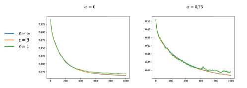
Figure 10: Training loss curve for the experiment of Figure 9. Each graph represents the training loss for a fixed value of $\alpha$ in (22) along the iterations of DP-SGD, for the different privacy budgets of the experiments.

B.3 Representation learning.

Finally, we present another completely novel application of our procedure: fair representation learning. Using the same data as before, the objective is to privately learn an encoder $\varphi_{\theta_{a}}$ and a decoder $\psi_{\theta_{b}}$ minimizing the reconstruction mean squared error of the reconstructed values, penalized with the sliced Wasserstein distance to alleviate unfairness present in the data. For simplicity, we denote $\theta=(\theta_{a},\theta_{b})$, $\varphi_{\theta}=\varphi_{\theta_{a}}$ and $\psi_{\theta}=\psi_{\theta_{b}}$. In our example, the encoder and decoder are defined as fully connected neural networks with two layers, hidden dimension 62 and bi-dimensional latent space, and we look for an encoded representation enhancing statistical parity by minimizing

$$\mathscr{L}^{SP}_{\alpha}(\varphi_{\theta},\psi_{\theta})=(1-\alpha)\frac{1}{n}\sum_{i=1}^{n}\|\psi_{\theta}(\varphi_{\theta}(x_{i}))-x_{i}\|_{2}^{2}+\alpha SW_{2}^{2}\Bigl{(}\varphi_{\theta}\#P_{\mathbf{X}_{0}},\varphi_{\theta}\#P_{\mathbf{X}_{1}}\Bigr{)}\ .$$ (23)

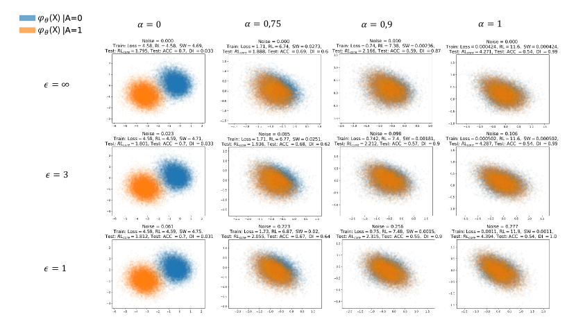
Figure 11: Plot of the latent space, $\varphi_{\theta}(X)$ conditioned by the sensitive attribute $A=0,1$ in the training set. $\theta$ is the parameter obtained after 500 iterations of DP-SGD minimizing (23) for the different values of $\alpha$ (columns), with different privacy budgets $\epsilon$ (rows) for $\delta=0.1/n$ fixed. The parameters of the optimization are the learning rate $=0.01$, clipping values $C=10,\ M=2,\ L=\sqrt{2}$, batch sizes $n_{0}^{\prime}\approx n_{0}/5,n_{1}^{\prime}\approx n_{1}/5$ and number of projections $=50$. Above each plot we indicate the noise added at each step of DP-SGD to obtain the desired privacy level, the value of the loss 23 in the training procedure, together with the individual value of the reconstruction loss (RL) and the sliced Wasserstein loss (SW). Last line includes the reconstruction loss on the core variables ($RL_{1}$), accuracy and disparate impact on test data.

As usual, Figure 11 presents the result of training this model for different values of $\alpha$ and $\epsilon$, with fixed $\delta=0.1/n$, number of iterations $T=500$ iterations, clipping values $C=10,M=2,L=\sqrt{2}$, learning rate $0.01$ and number of projections in the Monte Carlo approximation $=50$. Over each plot, we can see the noise introduced to achieve the required privacy level, the weighted and individual values of the loss during training, and other comparative measures computed with an independent test sample. First, $RL_{c}$ denotes the reconstruction loss in the core part $X_{core}$, i.e. the first eight variables of $X$. The rest of the variables $X_{sp}$ are just a noisy version of $A$. Thus, $RL_{c}$ provides a measure of the error in the reconstruction loss for the relevant part of the data, and Figure 11 shows that for increasing values of $\alpha$, even though the reconstruction loss increases significantly, the reconstruction associated with the core part is not affected much. The other measures computed on the test data are the accuracy and disparate impact of a simple logistic regression model trained on the encoded representation of a portion (60%) of the test data and evaluated on the remaining (40%). We observe that increasing values of $\alpha$ lead to values of the disparate impact index closer to 1, at the expense of a decrease in accuracy. Finally, we can infer from Figures 11 and 12 that privacy doesn’t affect much to the results of the optimization.

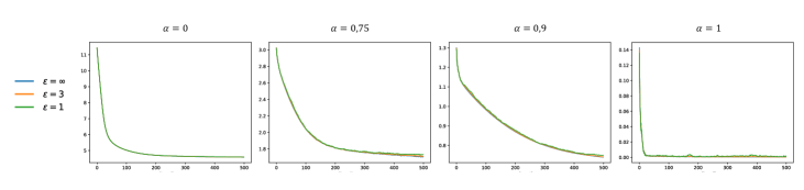
Figure 12: Training loss curve for the experiment of Figure 11. Each graph represents the training loss (23) for a fixed value of $\alpha$ along the iterations of DP-SGD, for the different privacy budgets of the experiments.

Appendix C Additional Experiments

To demonstrate the ability of our method to privately learn distributions in a deep learning scenario, we trained a neural network to approximate the distribution of a variable $Z$ by applying a transformation $g_{\theta}$ to another variable $X$. Specifically, we considered $n=100000$ samples of $Z$ drawn from the uniform distribution on a circle with radius $3/4$, and equal number of samples of $X$ drawn from the standard Gaussian distribution in $\mathbb{R}^{2}$. The function $g_{\theta}$ is defined as a fully connected neural network with an input dimension 2, three hidden layers with dimensions $(128,64,64)$, and an output dimension 2. Figure 13 shows the evolution of the matching problem at different training steps. Thanks to Theorem A.1, our methodology provides privacy guarantees for both the fixed variable $Z$ and the trained variable $X$, in the sense that $g_{\theta}$ is applied to $X$. Above each plot, we can see the iteration number, the value of the loss, and the privacy budget $\epsilon$ for both $X$ and $Z$, at each training step. The optimization parameters are $\delta=0.1/n$, batch size$=10,000$, learning rate $=0.0075$, number of projections in the Monte Carlo approximation $=50$, clipping values $M=1$ and $L=2\sqrt{2}$ (imposed using the suboptimal approach described in Remark A.2). To ensure more stable results, once we have privatized the gradient by adding noise, we clip the gradient again to improve the method’s stability. Note that this step preserves privacy due to the post-processing property. In comparison with the approach of (Rakotomamonjy & Ralaivola, 2021), which can only provide privacy guarantees with respect to the non-trained variable $Z$, our method provides privacy guarantees for both variables. Although privacy with respect to $Z$ might be sufficient in data generation, this example highlights the limitations of (Rakotomamonjy & Ralaivola, 2021), as their procedure cannot be applied in any situation where training is required on private data.

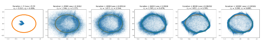
Figure 13: Data generation experiment in Appendix C. Samples from $X$ are represented in blue, samples from $Z$ in orange. Above each graph, we can see the iteration, the value of the loss, and privacy budgets w.r.t. the variables $X$ and $Z$.

Appendix D Counterexample for general cost functions

In this section, we demonstrate that we cannot bound in general the sensitivity of the gradient if we use the Wasserstein loss function $W_{p}$, for general $p\geq 1$. Following the notation of Theorem 4.1, we denote by $\mathbf{X}=\{x_{1},\ldots,x_{n}\}\subset\mathcal{X}^{n}$ the private dataset, $\mathbf{Z}=\{z_{1},\ldots,z_{n}\}\subset\mathbb{R}$ the non-private dataset, and $P_{\mathbf{X}},P_{\mathbf{Z}}$ the associated empirical distributions. Given $g_{\theta}:\mathcal{X}\rightarrow\mathbb{R}$ depending on the parameter $\theta$, and considering $h_{\theta}=I_{d}$, we study the sensitivity of $\Phi_{\theta}(\mathbf{X})=\nabla_{\theta}W_{p}(g_{\theta}\#P_{\mathbf{X}},P_{\mathbf{Z}})$, for the particular values of

• $\mathbf{X}=\{x_{1},\ldots,x_{n}\}$ with $x_{i}=\frac{i}{n},\ i\in[n]$

• $\mathbf{\tilde{X}}=\{\tilde{x}_{1},\ldots,\tilde{x}_{n}\}$ with $\tilde{x}_{i}=\frac{i-1}{n},\ i\in[n]$

• $\mathbf{Z}=\{z_{1},\ldots,z_{n}\}$, with $z_{i}=\frac{2i-1}{2n},\ i\in[n].$

• $g_{\theta}(x)=x+\theta$

For this particular choice, $\mathbf{X}\sim_{1}\mathbf{\tilde{X}}$, and Assumption 1 and 2 in Theorem 4.1 are verified for certain constants (once we restrict the domain of $\theta$). From the quantile representation, it is easy to compute

$$W_{p}(g_{\theta}\#P_{\mathbf{X}},P_{\mathbf{Z}})= \Bigl{(}\frac{1}{n}\sum_{i=1}^{n}|x_{i}+\theta-z_{i}|^{p}\Bigr{)}^{1/p}=\Bigl{(}\frac{1}{n}\sum_{i=1}^{n}\Big{|}\frac{1}{2n}+\theta\Big{|}^{p}\Bigr{)}^{1/p}=\left\{\begin{array}[]{cc}\frac{1}{2n}+\theta&\textnormal{if}\ \theta>-\frac{1}{2n}\\ -\theta-\frac{1}{2n}&\textnormal{if}\ \theta\leq-\frac{1}{2n}\end{array}\right.$$

$$W_{p}(g_{\theta}\#P_{\mathbf{\tilde{X}}},P_{\mathbf{Z}})= \Bigl{(}\frac{1}{n}\sum_{i=1}^{n}|\tilde{x}_{i}+\theta-z_{i}|^{p}\Bigr{)}^{1/p}=\Bigl{(}\frac{1}{n}\sum_{i=1}^{n}\Big{|}-\frac{1}{2n}+\theta\Big{|}^{p}\Bigr{)}^{1/p}=\left\{\begin{array}[]{cc}-\frac{1}{2n}+\theta&\textnormal{if}\ \theta>\frac{1}{2n}\\ \theta-\frac{1}{2n}&\textnormal{if}\ \theta\leq\frac{1}{2n}\end{array}\right.$$

Therefore, by setting $\theta=0$, we observe that the derivatives are $\Phi_{0}(\mathbf{X})=1$ and $\Phi_{0}(\mathbf{\tilde{X}})=-1$. Consequently, $\Delta\Phi_{\theta}\geq 2$, indicating that the sensitivity does not decrease with the sample size $n$.

References

- Abadi et al. (2015) Abadi, M., Agarwal, A., Barham, P., Brevdo, E., Chen, Z., Citro, C., Corrado, G. S., Davis, A., Dean, J., Devin, M., Ghemawat, S., Goodfellow, I., Harp, A., Irving, G., Isard, M., Jia, Y., Jozefowicz, R., Kaiser, L., Kudlur, M., Levenberg, J., Mané, D., Monga, R., Moore, S., Murray, D., Olah, C., Schuster, M., Shlens, J., Steiner, B., Sutskever, I., Talwar, K., Tucker, P., Vanhoucke, V., Vasudevan, V., Viégas, F., Vinyals, O., Warden, P., Wattenberg, M., Wicke, M., Yu, Y., and Zheng, X. TensorFlow: Large-scale machine learning on heterogeneous systems, 2015. URL https://www.tensorflow.org/. Software available from tensorflow.org.
- Abadi et al. (2016) Abadi, M., Chu, A., Goodfellow, I. J., McMahan, H. B., Mironov, I., Talwar, K., and Zhang, L. Deep learning with differential privacy. In Weippl, E. R., Katzenbeisser, S., Kruegel, C., Myers, A. C., and Halevi, S. (eds.), Proceedings of the 2016 ACM SIGSAC Conference on Computer and Communications Security, Vienna, Austria, October 24-28, 2016, pp. 308–318. ACM, 2016. doi: 10.1145/2976749.2978318. URL https://doi.org/10.1145/2976749.2978318.
- Abowd (2018) Abowd, J. M. The us census bureau adopts differential privacy. In Proceedings of the 24th ACM SIGKDD International Conference on Knowledge Discovery & Data Mining, pp. 2867–2867, 2018.
- Acharya et al. (2021) Acharya, J., Sun, Z., and Zhang, H. Differentially private Assouad, Fano, and Le Cam. In Feldman, V., Ligett, K., and Sabato, S. (eds.), Algorithmic Learning Theory, 16-19 March 2021, Virtual Conference, Worldwide, volume 132 of Proceedings of Machine Learning Research, pp. 48–78. PMLR, 2021. URL http://proceedings.mlr.press/v132/acharya21a.html.
- Aden-Ali et al. (2021) Aden-Ali, I., Ashtiani, H., and Kamath, G. On the sample complexity of privately learning unbounded high-dimensional gaussians. In Feldman, V., Ligett, K., and Sabato, S. (eds.), Algorithmic Learning Theory, 16-19 March 2021, Virtual Conference, Worldwide, volume 132 of Proceedings of Machine Learning Research, pp. 185–216. PMLR, 2021. URL http://proceedings.mlr.press/v132/aden-ali21a.html.
- Arjovsky et al. (2017) Arjovsky, M., Chintala, S., and Bottou, L. Wasserstein generative adversarial networks. In Precup, D. and Teh, Y. W. (eds.), Proceedings of the 34th International Conference on Machine Learning, ICML 2017, Sydney, NSW, Australia, 6-11 August 2017, volume 70 of Proceedings of Machine Learning Research, pp. 214–223. PMLR, 2017. URL http://proceedings.mlr.press/v70/arjovsky17a.html.
- Backstrom et al. (2007) Backstrom, L., Dwork, C., and Kleinberg, J. M. Wherefore art thou r3579x?: anonymized social networks, hidden patterns, and structural steganography. In Williamson, C. L., Zurko, M. E., Patel-Schneider, P. F., and Shenoy, P. J. (eds.), Proceedings of the 16th International Conference on World Wide Web, WWW 2007, Banff, Alberta, Canada, May 8-12, 2007, pp. 181–190. ACM, 2007. doi: 10.1145/1242572.1242598. URL https://doi.org/10.1145/1242572.1242598.
- Bagdasaryan et al. (2019) Bagdasaryan, E., Poursaeed, O., and Shmatikov, V. Differential privacy has disparate impact on model accuracy. In Wallach, H. M., Larochelle, H., Beygelzimer, A., d’Alché-Buc, F., Fox, E. B., and Garnett, R. (eds.), Advances in Neural Information Processing Systems 32: Annual Conference on Neural Information Processing Systems 2019, NeurIPS 2019, December 8-14, 2019, Vancouver, BC, Canada, pp. 15453–15462, 2019. URL https://proceedings.neurips.cc/paper/2019/hash/fc0de4e0396fff257ea362983c2dda5a-Abstract.html.
- Barber & Duchi (2014) Barber, R. F. and Duchi, J. C. Privacy and statistical risk: Formalisms and minimax bounds. CoRR, abs/1412.4451, 2014. URL http://arxiv.org/abs/1412.4451.
- Barocas et al. (2018) Barocas, S., Hardt, M., and Narayanan, A. Fairness and Machine Learning. fairmlbook.org, 2018. URL http://www.fairmlbook.org.
- Barrainkua et al. (2024) Barrainkua, A., Gordaliza, P., Lozano, J. A., and Quadrianto, N. Uncertainty matters: stable conclusions under unstable assessment of fairness results. In International Conference on Artificial Intelligence and Statistics, pp. 1198–1206. PMLR, 2024.
- Becker & Kohavi (1996) Becker, B. and Kohavi, R. Adult. UCI Machine Learning Repository, 1996. DOI: https://doi.org/10.24432/C5XW20.
- Besse et al. (2022) Besse, P., del Barrio, E., Gordaliza, P., Loubes, J.-M., and Risser, L. A survey of bias in machine learning through the prism of statistical parity. The American Statistician, 76(2):188–198, 2022.
- Biswas et al. (2020) Biswas, S., Dong, Y., Kamath, G., and Ullman, J. R. Coinpress: Practical private mean and covariance estimation. In Larochelle, H., Ranzato, M., Hadsell, R., Balcan, M., and Lin, H. (eds.), Advances in Neural Information Processing Systems 33: Annual Conference on Neural Information Processing Systems 2020, NeurIPS 2020, December 6-12, 2020, virtual, 2020. URL https://proceedings.neurips.cc/paper/2020/hash/a684eceee76fc522773286a895bc8436-Abstract.html.
- Bonneel et al. (2015) Bonneel, N., Rabin, J., Peyré, G., and Pfister, H. Sliced and radon wasserstein barycenters of measures. J. Math. Imaging Vis., 51(1):22–45, 2015. doi: 10.1007/S10851-014-0506-3. URL https://doi.org/10.1007/s10851-014-0506-3.
- Bradbury et al. (2018) Bradbury, J., Frostig, R., Hawkins, P., Johnson, M. J., Leary, C., Maclaurin, D., Necula, G., Paszke, A., VanderPlas, J., Wanderman-Milne, S., and Zhang, Q. JAX: composable transformations of Python+NumPy programs, 2018. URL http://github.com/jax-ml/jax.
- Brown et al. (2021) Brown, G., Gaboardi, M., Smith, A. D., Ullman, J. R., and Zakynthinou, L. Covariance-aware private mean estimation without private covariance estimation. In Ranzato, M., Beygelzimer, A., Dauphin, Y. N., Liang, P., and Vaughan, J. W. (eds.), Advances in Neural Information Processing Systems 34: Annual Conference on Neural Information Processing Systems 2021, NeurIPS 2021, December 6-14, 2021, virtual, pp. 7950–7964, 2021. URL https://proceedings.neurips.cc/paper/2021/hash/42778ef0b5805a96f9511e20b5611fce-Abstract.html.
- Bun et al. (2019) Bun, M., Kamath, G., Steinke, T., and Wu, Z. S. Private hypothesis selection. In Wallach, H. M., Larochelle, H., Beygelzimer, A., d’Alché-Buc, F., Fox, E. B., and Garnett, R. (eds.), Advances in Neural Information Processing Systems 32: Annual Conference on Neural Information Processing Systems 2019, NeurIPS 2019, December 8-14, 2019, Vancouver, BC, Canada, pp. 156–167, 2019. URL https://proceedings.neurips.cc/paper/2019/hash/9778d5d219c5080b9a6a17bef029331c-Abstract.html.
- Bun et al. (2021) Bun, M., Kamath, G., Steinke, T., and Wu, Z. S. Private hypothesis selection. IEEE Trans. Inf. Theory, 67(3):1981–2000, 2021. doi: 10.1109/TIT.2021.3049802. URL https://doi.org/10.1109/TIT.2021.3049802.
- Cai et al. (2019) Cai, T. T., Wang, Y., and Zhang, L. The cost of privacy: Optimal rates of convergence for parameter estimation with differential privacy. CoRR, abs/1902.04495, 2019. URL http://arxiv.org/abs/1902.04495.
- Chiappa et al. (2020) Chiappa, S., Jiang, R., Stepleton, T., Pacchiano, A., Jiang, H., and Aslanides, J. A general approach to fairness with optimal transport. In The Thirty-Fourth AAAI Conference on Artificial Intelligence, AAAI 2020, The Thirty-Second Innovative Applications of Artificial Intelligence Conference, IAAI 2020, The Tenth AAAI Symposium on Educational Advances in Artificial Intelligence, EAAI 2020, New York, NY, USA, February 7-12, 2020, pp. 3633–3640. AAAI Press, 2020. doi: 10.1609/AAAI.V34I04.5771. URL https://doi.org/10.1609/aaai.v34i04.5771.
- Chouldechova & Roth (2020) Chouldechova, A. and Roth, A. A snapshot of the frontiers of fairness in machine learning. Communications of the ACM, 63(5):82–89, 2020.
- Chzhen et al. (2020) Chzhen, E., Denis, C., Hebiri, M., Oneto, L., and Pontil, M. Fair regression with wasserstein barycenters. In Larochelle, H., Ranzato, M., Hadsell, R., Balcan, M., and Lin, H. (eds.), Advances in Neural Information Processing Systems, volume 33, pp. 7321–7331. Curran Associates, Inc., 2020. URL https://proceedings.neurips.cc/paper_files/paper/2020/file/51cdbd2611e844ece5d80878eb770436-Paper.pdf.
- Courty et al. (2017) Courty, N., Flamary, R., Tuia, D., and Rakotomamonjy, A. Optimal transport for domain adaptation. IEEE Trans. Pattern Anal. Mach. Intell., 39(9):1853–1865, 2017. doi: 10.1109/TPAMI.2016.2615921. URL https://doi.org/10.1109/TPAMI.2016.2615921.
- Cummings et al. (2019) Cummings, R., Gupta, V., Kimpara, D., and Morgenstern, J. On the compatibility of privacy and fairness. In Adjunct publication of the 27th conference on user modeling, adaptation and personalization, pp. 309–315, 2019.
- Cuturi (2013) Cuturi, M. Sinkhorn distances: Lightspeed computation of optimal transport. In Burges, C. J. C., Bottou, L., Ghahramani, Z., and Weinberger, K. Q. (eds.), Advances in Neural Information Processing Systems 26: 27th Annual Conference on Neural Information Processing Systems 2013. Proceedings of a meeting held December 5-8, 2013, Lake Tahoe, Nevada, United States, pp. 2292–2300, 2013. URL https://proceedings.neurips.cc/paper/2013/hash/af21d0c97db2e27e13572cbf59eb343d-Abstract.html.
- De Lara et al. (2024) De Lara, L., González-Sanz, A., Asher, N., Risser, L., and Loubes, J.-M. Transport-based counterfactual models. Journal of Machine Learning Research, 25(136):1–59, 2024.
- Deshpande et al. (2018) Deshpande, I., Zhang, Z., and Schwing, A. G. Generative modeling using the sliced wasserstein distance. In 2018 IEEE Conference on Computer Vision and Pattern Recognition, CVPR 2018, Salt Lake City, UT, USA, June 18-22, 2018, pp. 3483–3491. Computer Vision Foundation / IEEE Computer Society, 2018. doi: 10.1109/CVPR.2018.00367. URL http://openaccess.thecvf.com/content_cvpr_2018/html/Deshpande_Generative_Modeling_Using_CVPR_2018_paper.html.
- Diakonikolas et al. (2015) Diakonikolas, I., Hardt, M., and Schmidt, L. Differentially private learning of structured discrete distributions. In Cortes, C., Lawrence, N. D., Lee, D. D., Sugiyama, M., and Garnett, R. (eds.), Advances in Neural Information Processing Systems 28: Annual Conference on Neural Information Processing Systems 2015, December 7-12, 2015, Montreal, Quebec, Canada, pp. 2566–2574, 2015. URL https://proceedings.neurips.cc/paper/2015/hash/2b3bf3eee2475e03885a110e9acaab61-Abstract.html.
- Ding et al. (2017) Ding, B., Kulkarni, J., and Yekhanin, S. Collecting telemetry data privately. In Guyon, I., von Luxburg, U., Bengio, S., Wallach, H. M., Fergus, R., Vishwanathan, S. V. N., and Garnett, R. (eds.), Advances in Neural Information Processing Systems 30: Annual Conference on Neural Information Processing Systems 2017, December 4-9, 2017, Long Beach, CA, USA, pp. 3571–3580, 2017. URL https://proceedings.neurips.cc/paper/2017/hash/253614bbac999b38b5b60cae531c4969-Abstract.html.
- Ding et al. (2020) Ding, J., Zhang, X., Li, X., Wang, J., Yu, R., and Pan, M. Differentially private and fair classification via calibrated functional mechanism. In The Thirty-Fourth AAAI Conference on Artificial Intelligence, AAAI 2020, The Thirty-Second Innovative Applications of Artificial Intelligence Conference, IAAI 2020, The Tenth AAAI Symposium on Educational Advances in Artificial Intelligence, EAAI 2020, New York, NY, USA, February 7-12, 2020, pp. 622–629. AAAI Press, 2020. doi: 10.1609/AAAI.V34I01.5402. URL https://doi.org/10.1609/aaai.v34i01.5402.
- Dinur & Nissim (2003) Dinur, I. and Nissim, K. Revealing information while preserving privacy. In Neven, F., Beeri, C., and Milo, T. (eds.), Proceedings of the Twenty-Second ACM SIGACT-SIGMOD-SIGART Symposium on Principles of Database Systems, June 9-12, 2003, San Diego, CA, USA, pp. 202–210. ACM, 2003. doi: 10.1145/773153.773173. URL https://doi.org/10.1145/773153.773173.
- Dong et al. (2019) Dong, J., Roth, A., and Su, W. J. Gaussian differential privacy. CoRR, abs/1905.02383, 2019. URL http://arxiv.org/abs/1905.02383.
- Dwork (2006) Dwork, C. Differential privacy. In Bugliesi, M., Preneel, B., Sassone, V., and Wegener, I. (eds.), Automata, Languages and Programming, 33rd International Colloquium, ICALP 2006, Venice, Italy, July 10-14, 2006, Proceedings, Part II, volume 4052 of Lecture Notes in Computer Science, pp. 1–12. Springer, 2006. doi: 10.1007/11787006“˙1. URL https://doi.org/10.1007/11787006_1.
- Dwork & Roth (2014) Dwork, C. and Roth, A. The algorithmic foundations of differential privacy. Found. Trends Theor. Comput. Sci., 9(3-4):211–407, 2014. doi: 10.1561/0400000042. URL https://doi.org/10.1561/0400000042.
- Dwork et al. (2006a) Dwork, C., Kenthapadi, K., McSherry, F., Mironov, I., and Naor, M. Our data, ourselves: Privacy via distributed noise generation. In Vaudenay, S. (ed.), Advances in Cryptology - EUROCRYPT 2006, 25th Annual International Conference on the Theory and Applications of Cryptographic Techniques, St. Petersburg, Russia, May 28 - June 1, 2006, Proceedings, volume 4004 of Lecture Notes in Computer Science, pp. 486–503. Springer, 2006a. doi: 10.1007/11761679“˙29. URL https://doi.org/10.1007/11761679_29.
- Dwork et al. (2006b) Dwork, C., McSherry, F., Nissim, K., and Smith, A. D. Calibrating noise to sensitivity in private data analysis. In Halevi, S. and Rabin, T. (eds.), Theory of Cryptography, Third Theory of Cryptography Conference, TCC 2006, New York, NY, USA, March 4-7, 2006, Proceedings, volume 3876 of Lecture Notes in Computer Science, pp. 265–284. Springer, 2006b. doi: 10.1007/11681878“˙14. URL https://doi.org/10.1007/11681878_14.
- Dwork et al. (2012) Dwork, C., Hardt, M., Pitassi, T., Reingold, O., and Zemel, R. Fairness through awareness. In Proceedings of the 3rd innovations in theoretical computer science conference, pp. 214–226, 2012.
- Erlingsson et al. (2014) Erlingsson, Ú., Pihur, V., and Korolova, A. RAPPOR: randomized aggregatable privacy-preserving ordinal response. In Ahn, G., Yung, M., and Li, N. (eds.), Proceedings of the 2014 ACM SIGSAC Conference on Computer and Communications Security, Scottsdale, AZ, USA, November 3-7, 2014, pp. 1054–1067. ACM, 2014. doi: 10.1145/2660267.2660348. URL https://doi.org/10.1145/2660267.2660348.
- Esipova et al. (2023) Esipova, M. S., Ghomi, A. A., Luo, Y., and Cresswell, J. C. Disparate impact in differential privacy from gradient misalignment. In The Eleventh International Conference on Learning Representations, ICLR 2023, Kigali, Rwanda, May 1-5, 2023. OpenReview.net, 2023. URL https://openreview.net/forum?id=qLOaeRvteqbx.
- Farrand et al. (2020) Farrand, T., Mireshghallah, F., Singh, S., and Trask, A. Neither private nor fair: Impact of data imbalance on utility and fairness in differential privacy. In Zhang, B., Popa, R. A., Zaharia, M., Gu, G., and Ji, S. (eds.), PPMLP’20: Proceedings of the 2020 Workshop on Privacy-Preserving Machine Learning in Practice, Virtual Event, USA, November, 2020, pp. 15–19. ACM, 2020. doi: 10.1145/3411501.3419419. URL https://doi.org/10.1145/3411501.3419419.
- Feldman et al. (2015) Feldman, M., Friedler, S. A., Moeller, J., Scheidegger, C., and Venkatasubramanian, S. Certifying and removing disparate impact. In proceedings of the 21th ACM SIGKDD international conference on knowledge discovery and data mining, pp. 259–268, 2015.
- Fioretto et al. (2022) Fioretto, F., Tran, C., Hentenryck, P. V., and Zhu, K. Differential privacy and fairness in decisions and learning tasks: A survey. In Raedt, L. D. (ed.), Proceedings of the Thirty-First International Joint Conference on Artificial Intelligence, IJCAI 2022, Vienna, Austria, 23-29 July 2022, pp. 5470–5477. ijcai.org, 2022. doi: 10.24963/IJCAI.2022/766. URL https://doi.org/10.24963/ijcai.2022/766.
- Fredrikson et al. (2015) Fredrikson, M., Jha, S., and Ristenpart, T. Model inversion attacks that exploit confidence information and basic countermeasures. In Ray, I., Li, N., and Kruegel, C. (eds.), Proceedings of the 22nd ACM SIGSAC Conference on Computer and Communications Security, Denver, CO, USA, October 12-16, 2015, pp. 1322–1333. ACM, 2015. doi: 10.1145/2810103.2813677. URL https://doi.org/10.1145/2810103.2813677.
- Gaucher et al. (2023) Gaucher, S., Schreuder, N., and Chzhen, E. Fair learning with wasserstein barycenters for non-decomposable performance measures. In International Conference on Artificial Intelligence and Statistics, pp. 2436–2459. PMLR, 2023.
- Ghoukasian & Asoodeh (2024) Ghoukasian, H. and Asoodeh, S. Differentially private fair binary classifications. CoRR, abs/2402.15603, 2024. doi: 10.48550/ARXIV.2402.15603. URL https://doi.org/10.48550/arXiv.2402.15603.
- Gordaliza et al. (2019) Gordaliza, P., del Barrio, E., Gamboa, F., and Loubes, J. Obtaining fairness using optimal transport theory. In Chaudhuri, K. and Salakhutdinov, R. (eds.), Proceedings of the 36th International Conference on Machine Learning, ICML 2019, 9-15 June 2019, Long Beach, California, USA, volume 97 of Proceedings of Machine Learning Research, pp. 2357–2365. PMLR, 2019. URL http://proceedings.mlr.press/v97/gordaliza19a.html.
- Gouic et al. (2020) Gouic, T. L., Loubes, J.-M., and Rigollet, P. Projection to fairness in statistical learning. arXiv preprint arXiv:2005.11720, 2020.
- Harder et al. (2021) Harder, F., Adamczewski, K., and Park, M. Dp-merf: Differentially private mean embeddings with randomfeatures for practical privacy-preserving data generation. In International conference on artificial intelligence and statistics, pp. 1819–1827. PMLR, 2021.
- Hofmann (1994) Hofmann, H. Statlog (German Credit Data). UCI Machine Learning Repository, 1994. DOI: https://doi.org/10.24432/C5NC77.
- Homer et al. (2008) Homer, N., Szelinger, S., Redman, M., Duggan, D., Tembe, W., Muehling, J., Pearson, J. V., Stephan, D. A., Nelson, S. F., and Craig, D. W. Resolving individuals contributing trace amounts of dna to highly complex mixtures using high-density snp genotyping microarrays. PLoS Genet, 4(8):e1000167, 2008.
- Jagielski et al. (2019) Jagielski, M., Kearns, M., Mao, J., Oprea, A., Roth, A., Sharifi-Malvajerdi, S., and Ullman, J. Differentially private fair learning. In International Conference on Machine Learning, pp. 3000–3008. PMLR, 2019.
- Jiang et al. (2020) Jiang, R., Pacchiano, A., Stepleton, T., Jiang, H., and Chiappa, S. Wasserstein fair classification. In Uncertainty in artificial intelligence, pp. 862–872. PMLR, 2020.
- Kamath et al. (2019) Kamath, G., Li, J., Singhal, V., and Ullman, J. R. Privately learning high-dimensional distributions. In Beygelzimer, A. and Hsu, D. (eds.), Conference on Learning Theory, COLT 2019, 25-28 June 2019, Phoenix, AZ, USA, volume 99 of Proceedings of Machine Learning Research, pp. 1853–1902. PMLR, 2019. URL http://proceedings.mlr.press/v99/kamath19a.html.
- Kamath et al. (2020) Kamath, G., Singhal, V., and Ullman, J. R. Private mean estimation of heavy-tailed distributions. In Abernethy, J. D. and Agarwal, S. (eds.), Conference on Learning Theory, COLT 2020, 9-12 July 2020, Virtual Event [Graz, Austria], volume 125 of Proceedings of Machine Learning Research, pp. 2204–2235. PMLR, 2020. URL http://proceedings.mlr.press/v125/kamath20a.html.
- Kamath et al. (2022a) Kamath, G., Liu, X., and Zhang, H. Improved rates for differentially private stochastic convex optimization with heavy-tailed data. In Chaudhuri, K., Jegelka, S., Song, L., Szepesvári, C., Niu, G., and Sabato, S. (eds.), International Conference on Machine Learning, ICML 2022, 17-23 July 2022, Baltimore, Maryland, USA, volume 162 of Proceedings of Machine Learning Research, pp. 10633–10660. PMLR, 2022a. URL https://proceedings.mlr.press/v162/kamath22a.html.
- Kamath et al. (2022b) Kamath, G., Mouzakis, A., and Singhal, V. New lower bounds for private estimation and a generalized fingerprinting lemma. In NeurIPS, 2022b. URL http://papers.nips.cc/paper_files/paper/2022/hash/9a6b278218966499194491f55ccf8b75-Abstract-Conference.html.
- Kamath et al. (2023) Kamath, G., Mouzakis, A., Regehr, M., Singhal, V., Steinke, T., and Ullman, J. R. A bias-variance-privacy trilemma for statistical estimation. CoRR, abs/2301.13334, 2023. doi: 10.48550/ARXIV.2301.13334. URL https://doi.org/10.48550/arXiv.2301.13334.
- Karwa & Vadhan (2018) Karwa, V. and Vadhan, S. P. Finite sample differentially private confidence intervals. In Karlin, A. R. (ed.), 9th Innovations in Theoretical Computer Science Conference, ITCS 2018, January 11-14, 2018, Cambridge, MA, USA, volume 94 of LIPIcs, pp. 44:1–44:9. Schloss Dagstuhl - Leibniz-Zentrum für Informatik, 2018. doi: 10.4230/LIPIcs.ITCS.2018.44. URL https://doi.org/10.4230/LIPIcs.ITCS.2018.44.
- Kawamoto & Murakami (2019) Kawamoto, Y. and Murakami, T. Local obfuscation mechanisms for hiding probability distributions. In Sako, K., Schneider, S. A., and Ryan, P. Y. A. (eds.), Computer Security - ESORICS 2019 - 24th European Symposium on Research in Computer Security, Luxembourg, September 23-27, 2019, Proceedings, Part I, volume 11735 of Lecture Notes in Computer Science, pp. 128–148. Springer, 2019. doi: 10.1007/978-3-030-29959-0“˙7. URL https://doi.org/10.1007/978-3-030-29959-0_7.
- Kolouri et al. (2018) Kolouri, S., Martin, C. E., and Rohde, G. K. Sliced-wasserstein autoencoder: An embarrassingly simple generative model. CoRR, abs/1804.01947, 2018. URL http://arxiv.org/abs/1804.01947.
- Krco et al. (2025) Krco, N., Laugel, T., Loubes, J.-M., and Detyniecki, M. When mitigating bias is unfair: A comprehensive study on the impact of bias mitigation algorithms. arXiv preprint arXiv:2302.07185, IEEE SATML, 2025.
- Lalanne (2023) Lalanne, C. On the tradeoffs of statistical learning with privacy. Theses, Ecole normale supérieure de lyon - ENS LYON, October 2023. URL https://theses.hal.science/tel-04379624.
- Lalanne & Gadat (2024) Lalanne, C. and Gadat, S. Privately Learning Smooth Distributions on the Hypercube by Projections. In ICML 2024 - 41st International Conference on Machine Learning, pp. 39 p., Vienna, Austria, July 2024. URL https://hal.science/hal-04549279.
- Lalanne et al. (2023a) Lalanne, C., Garivier, A., and Gribonval, R. Private Statistical Estimation of Many Quantiles. In ICML 2023 - 40th International Conference on Machine Learning, Honolulu, United States, July 2023a. URL https://hal.science/hal-03986170.
- Lalanne et al. (2023b) Lalanne, C., Gastaud, C., Grislain, N., Garivier, A., and Gribonval, R. Private Quantiles Estimation in the Presence of Atoms. Information and Inference, August 2023b. doi: 10.1093/imaiai/iaad030. URL https://hal.science/hal-03572701.
- Lee et al. (2019) Lee, C., Batra, T., Baig, M. H., and Ulbricht, D. Sliced wasserstein discrepancy for unsupervised domain adaptation. In IEEE Conference on Computer Vision and Pattern Recognition, CVPR 2019, Long Beach, CA, USA, June 16-20, 2019, pp. 10285–10295. Computer Vision Foundation / IEEE, 2019. doi: 10.1109/CVPR.2019.01053. URL http://openaccess.thecvf.com/content_CVPR_2019/html/Lee_Sliced_Wasserstein_Discrepancy_for_Unsupervised_Domain_Adaptation_CVPR_2019_paper.html.
- Liu et al. (2025) Liu, Z., Yu, H., Chen, K., and Li, A. Privacy-preserving generative modeling with sliced wasserstein distance. IEEE Trans. Inf. Forensics Secur., 20:1011–1022, 2025. doi: 10.1109/TIFS.2024.3516549. URL https://doi.org/10.1109/TIFS.2024.3516549.
- Loukides et al. (2010) Loukides, G., Denny, J. C., and Malin, B. A. The disclosure of diagnosis codes can breach research participants’ privacy. J. Am. Medical Informatics Assoc., 17(3):322–327, 2010. doi: 10.1136/jamia.2009.002725. URL https://doi.org/10.1136/jamia.2009.002725.
- Lowy et al. (2022) Lowy, A., Gupta, D., and Razaviyayn, M. Stochastic differentially private and fair learning. CoRR, abs/2210.08781, 2022. doi: 10.48550/ARXIV.2210.08781. URL https://doi.org/10.48550/arXiv.2210.08781.
- Mangold et al. (2023) Mangold, P., Perrot, M., Bellet, A., and Tommasi, M. Differential privacy has bounded impact on fairness in classification. In Krause, A., Brunskill, E., Cho, K., Engelhardt, B., Sabato, S., and Scarlett, J. (eds.), International Conference on Machine Learning, ICML 2023, 23-29 July 2023, Honolulu, Hawaii, USA, volume 202 of Proceedings of Machine Learning Research, pp. 23681–23705. PMLR, 2023. URL https://proceedings.mlr.press/v202/mangold23a.html.
- Narayanan & Shmatikov (2006) Narayanan, A. and Shmatikov, V. How to break anonymity of the netflix prize dataset. CoRR, abs/cs/0610105, 2006. URL http://arxiv.org/abs/cs/0610105.
- Narayanan & Shmatikov (2008) Narayanan, A. and Shmatikov, V. Robust de-anonymization of large sparse datasets. In 2008 IEEE Symposium on Security and Privacy (S&P 2008), 18-21 May 2008, Oakland, California, USA, pp. 111–125. IEEE Computer Society, 2008. doi: 10.1109/SP.2008.33. URL https://doi.org/10.1109/SP.2008.33.
- Oneto & Chiappa (2020) Oneto, L. and Chiappa, S. Fairness in machine learning. In Recent trends in learning from data: Tutorials from the inns big data and deep learning conference (innsbddl2019), pp. 155–196. Springer, 2020.
- Paszke et al. (2019) Paszke, A., Gross, S., Massa, F., Lerer, A., Bradbury, J., Chanan, G., Killeen, T., Lin, Z., Gimelshein, N., Antiga, L., Desmaison, A., Kopf, A., Yang, E., DeVito, Z., Raison, M., Tejani, A., Chilamkurthy, S., Steiner, B., Fang, L., Bai, J., and Chintala, S. Pytorch: An imperative style, high-performance deep learning library. In Advances in Neural Information Processing Systems 32, pp. 8024–8035. Curran Associates, Inc., 2019. URL http://papers.neurips.cc/paper/9015-pytorch-an-imperative-style-high-performance-deep-learning-library.pdf.
- Pierquin et al. (2024) Pierquin, C., Bellet, A., Tommasi, M., and Boussard, M. Rényi pufferfish privacy: General additive noise mechanisms and privacy amplification by iteration via shift reduction lemmas. In Forty-first International Conference on Machine Learning, ICML 2024, Vienna, Austria, July 21-27, 2024. OpenReview.net, 2024. URL https://openreview.net/forum?id=VZsxhPpu9T.
- Rabin et al. (2011) Rabin, J., Peyré, G., Delon, J., and Bernot, M. Wasserstein barycenter and its application to texture mixing. In Bruckstein, A. M., ter Haar Romeny, B. M., Bronstein, A. M., and Bronstein, M. M. (eds.), Scale Space and Variational Methods in Computer Vision - Third International Conference, SSVM 2011, Ein-Gedi, Israel, May 29 - June 2, 2011, Revised Selected Papers, volume 6667 of Lecture Notes in Computer Science, pp. 435–446. Springer, 2011. doi: 10.1007/978-3-642-24785-9“˙37. URL https://doi.org/10.1007/978-3-642-24785-9_37.
- Rakotomamonjy & Ralaivola (2021) Rakotomamonjy, A. and Ralaivola, L. Differentially private sliced wasserstein distance. In Meila, M. and Zhang, T. (eds.), Proceedings of the 38th International Conference on Machine Learning, ICML 2021, 18-24 July 2021, Virtual Event, volume 139 of Proceedings of Machine Learning Research, pp. 8810–8820. PMLR, 2021. URL http://proceedings.mlr.press/v139/rakotomamonjy21a.html.
- Risser et al. (2022) Risser, L., González-Sanz, A., Vincenot, Q., and Loubes, J. Tackling algorithmic bias in neural-network classifiers using wasserstein-2 regularization. J. Math. Imaging Vis., 64(6):672–689, 2022. doi: 10.1007/S10851-022-01090-2. URL https://doi.org/10.1007/s10851-022-01090-2.
- Sebag et al. (2023) Sebag, I., Pydi, M. S., Franceschi, J., Rakotomamonjy, A., Gartrell, M., Atif, J., and Allauzen, A. Differentially private gradient flow based on the sliced wasserstein distance for non-parametric generative modeling. CoRR, abs/2312.08227, 2023. doi: 10.48550/ARXIV.2312.08227. URL https://doi.org/10.48550/arXiv.2312.08227.
- Singhal (2023) Singhal, V. A polynomial time, pure differentially private estimator for binary product distributions. CoRR, abs/2304.06787, 2023. doi: 10.48550/ARXIV.2304.06787. URL https://doi.org/10.48550/arXiv.2304.06787.
- Steinke (2022) Steinke, T. Composition of differential privacy & privacy amplification by subsampling. CoRR, abs/2210.00597, 2022. doi: 10.48550/ARXIV.2210.00597. URL https://doi.org/10.48550/arXiv.2210.00597.
- Sweeney (2000) Sweeney, L. Simple demographics often identify people uniquely. Health (San Francisco), 671(2000):1–34, 2000.
- Sweeney (2002) Sweeney, L. k-anonymity: A model for protecting privacy. Int. J. Uncertain. Fuzziness Knowl. Based Syst., 10(5):557–570, 2002. doi: 10.1142/S0218488502001648. URL https://doi.org/10.1142/S0218488502001648.
- Tanguy et al. (2023) Tanguy, E., Flamary, R., and Delon, J. Properties of discrete sliced wasserstein losses. CoRR, abs/2307.10352, 2023. doi: 10.48550/ARXIV.2307.10352. URL https://doi.org/10.48550/arXiv.2307.10352.
- Thakurta et al. (2017) Thakurta, A. G., Vyrros, A. H., Vaishampayan, U. S., Kapoor, G., Freudiger, J., Sridhar, V. R., and Davidson, D. Learning new words. Granted US Patents, 9594741, 2017.
- Tien et al. (2019) Tien, N. L., Habrard, A., and Sebban, M. Differentially private optimal transport: Application to domain adaptation. In Kraus, S. (ed.), Proceedings of the Twenty-Eighth International Joint Conference on Artificial Intelligence, IJCAI 2019, Macao, China, August 10-16, 2019, pp. 2852–2858. ijcai.org, 2019. doi: 10.24963/IJCAI.2019/395. URL https://doi.org/10.24963/ijcai.2019/395.
- Tolstikhin et al. (2018) Tolstikhin, I. O., Bousquet, O., Gelly, S., and Schölkopf, B. Wasserstein auto-encoders. In 6th International Conference on Learning Representations, ICLR 2018, Vancouver, BC, Canada, April 30 - May 3, 2018, Conference Track Proceedings. OpenReview.net, 2018. URL https://openreview.net/forum?id=HkL7n1-0b.
- Tran et al. (2021) Tran, C., Dinh, M. H., and Fioretto, F. Differentially private empirical risk minimization under the fairness lens. In Ranzato, M., Beygelzimer, A., Dauphin, Y. N., Liang, P., and Vaughan, J. W. (eds.), Advances in Neural Information Processing Systems 34: Annual Conference on Neural Information Processing Systems 2021, NeurIPS 2021, December 6-14, 2021, virtual, pp. 27555–27565, 2021. URL https://proceedings.neurips.cc/paper/2021/hash/e7e8f8e5982b3298c8addedf6811d500-Abstract.html.
- Wagner & Eckhoff (2018) Wagner, I. and Eckhoff, D. Technical privacy metrics: A systematic survey. ACM Comput. Surv., 51(3):57:1–57:38, 2018. doi: 10.1145/3168389. URL https://doi.org/10.1145/3168389.
- Wang et al. (2022) Wang, X., Zhang, Y., and Zhu, R. A brief review on algorithmic fairness. Management System Engineering, 1(1):7, 2022. ISSN 2731-5843. doi: 10.1007/s44176-022-00006-z. URL https://doi.org/10.1007/s44176-022-00006-z.
- Wasserman & Zhou (2010) Wasserman, L. A. and Zhou, S. A statistical framework for differential privacy. Journal of the American Statistical Association, 105(489):375–389, 2010. doi: 10.1198/jasa.2009.tm08651. URL https://doi.org/10.1198/jasa.2009.tm08651.
- Wu et al. (2019) Wu, J., Huang, Z., Acharya, D., Li, W., Thoma, J., Paudel, D. P., and Gool, L. V. Sliced wasserstein generative models. In IEEE Conference on Computer Vision and Pattern Recognition, CVPR 2019, Long Beach, CA, USA, June 16-20, 2019, pp. 3713–3722. Computer Vision Foundation / IEEE, 2019. doi: 10.1109/CVPR.2019.00383. URL http://openaccess.thecvf.com/content_CVPR_2019/html/Wu_Sliced_Wasserstein_Generative_Models_CVPR_2019_paper.html.
- Xian et al. (2024) Xian, R., Li, Q., Kamath, G., and Zhao, H. Differentially private post-processing for fair regression. In Forty-first International Conference on Machine Learning, ICML 2024, Vienna, Austria, July 21-27, 2024. OpenReview.net, 2024. URL https://openreview.net/forum?id=JNeeRjKbuH.
- Xu et al. (2019) Xu, D., Yuan, S., and Wu, X. Achieving differential privacy and fairness in logistic regression. In Amer-Yahia, S., Mahdian, M., Goel, A., Houben, G., Lerman, K., McAuley, J. J., Baeza-Yates, R., and Zia, L. (eds.), Companion of The 2019 World Wide Web Conference, WWW 2019, San Francisco, CA, USA, May 13-17, 2019, pp. 594–599. ACM, 2019. doi: 10.1145/3308560.3317584. URL https://doi.org/10.1145/3308560.3317584.
- Xu et al. (2021) Xu, D., Du, W., and Wu, X. Removing disparate impact on model accuracy in differentially private stochastic gradient descent. In Zhu, F., Ooi, B. C., and Miao, C. (eds.), KDD ’21: The 27th ACM SIGKDD Conference on Knowledge Discovery and Data Mining, Virtual Event, Singapore, August 14-18, 2021, pp. 1924–1932. ACM, 2021. doi: 10.1145/3447548.3467268. URL https://doi.org/10.1145/3447548.3467268.
- Yaghini et al. (2023) Yaghini, M., Liu, P., Boenisch, F., and Papernot, N. Learning with impartiality to walk on the pareto frontier of fairness, privacy, and utility. arXiv preprint arXiv:2302.09183, 2023.
- Yang et al. (2024) Yang, C., Qi, J., and Zhou, A. Wasserstein differential privacy. In Wooldridge, M. J., Dy, J. G., and Natarajan, S. (eds.), Thirty-Eighth AAAI Conference on Artificial Intelligence, AAAI 2024, Thirty-Sixth Conference on Innovative Applications of Artificial Intelligence, IAAI 2024, Fourteenth Symposium on Educational Advances in Artificial Intelligence, EAAI 2014, February 20-27, 2024, Vancouver, Canada, pp. 16299–16307. AAAI Press, 2024. doi: 10.1609/AAAI.V38I15.29565. URL https://doi.org/10.1609/aaai.v38i15.29565.
- Yousefpour et al. (2021) Yousefpour, A., Shilov, I., Sablayrolles, A., Testuggine, D., Prasad, K., Malek, M., Nguyen, J., Ghosh, S., Bharadwaj, A., Zhao, J., Cormode, G., and Mironov, I. Opacus: User-friendly differential privacy library in PyTorch. arXiv preprint arXiv:2109.12298, 2021.