Predicting Steady-State Behavior in Complex Networks with Graph Neural Networks

Abstract

In complex systems, information propagation can be defined as diffused or delocalized, weakly localized, and strongly localized. This study investigates the application of graph neural network models to learn the behavior of a linear dynamical system on networks. A graph convolution and attention-based neural network framework has been developed to identify the steady-state behavior of the linear dynamical system. We reveal that our trained model distinguishes the different states with high accuracy. Furthermore, we have evaluated model performance with real-world data. In addition, to understand the explainability of our model, we provide an analytical derivation for the forward and backward propagation of our framework.

I Introduction

Relations or interactions are ubiquitous, whether the interaction of power grid generators to provide proper functioning of the power supply over a country, or interactions of bio-molecules inside the cell to the proper functioning of cellular activity, or interactions of neurons inside brains to perform specific functions or interactions among satellites to provide accurate GPS services or interactions among quantum particle enabling quantum communications or the recent coronavirus spread  [1, 2, 3, 4, 5]. All these systems share two fundamental characteristics: a network structure and information propagation among their components.

In complex networks, information propagation can occur in three distinct states - diffused or delocalized, weakly localized, and strongly localized [6]. Localization refers to the tendency of information to condense in a single component (strong localization) or a few components (weak localization) of the network instead of information diffusing evenly (delocalization) throughout the network (Fig. 1). Localization or lack of it is particularly significant in solid-state physics and quantum chemistry [7], where the presence or absence of localization influences the properties of molecules and materials. For example, electrons are delocalized in metals, while in insulators, they are localized [7].

Investigation of (de)localization behavior of complex networks is important for gaining insight into fundamental network problems such as network centrality measure [8], spectral partitioning [9], development of approximation algorithms [10]. Additionally, it plays a vital role in understanding a wide range of diffusion processes, like criticality in brain networks, epidemic spread, and rumor propagation [11, 12]. These dynamic processes have an impact on how different complex systems evolve or behave [12]. For example, understanding epidemic spread can help in developing strategies to slow its initial transmission, allowing time for vaccine development and deployment [13, 14, 15, 16, 17]. The interactions within real-world complex systems are often nonlinear [18]. In some cases, nonlinear systems can be solved by transforming them into linear systems through changing variables. Furthermore, the behavior of nonlinear systems can frequently be approximated by their linear counterparts near fixed points. Therefore, understanding linear systems and their solutions is an essential first step toward comprehending more complex nonlinear dynamical systems [18].

Here, we develop a Graph Neural Network (GNN) architecture to identify the behavior of linear dynamical states on complex networks. We create datasets where the training labels are derived from the inverse participation ratio (IPR) value of the principal eigenvector (PEV) of the network matrices. The GNN model takes the network structure as input and predicts IPR values, enabling the identification of graphs into their respective linear dynamical states. Our model performs well in identifying different states and is particularly effective across varying-sized networks. A key advantage of using GNN is its ability to train on smaller networks and generalize well to larger ones during testing. We also provide an analytical framework to understand the explainability of our model. Finally, we use real-world data sets in our model.

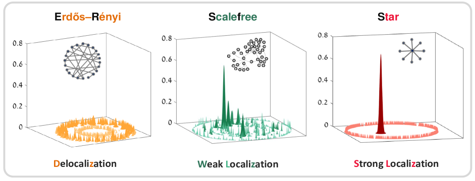
Figure 1: Steady-state behavior in linear dynamical systems on complex networks. We depict the nodes in the graphs with $x-y$ coordinates. We assign the sizes of a node based on the degree of a node. The $z-axis$ portrays the amount of information ($x_{i}^{*}$) on a node in the steady state. The steady-state behavior of linear dynamics on the ER random network leads to delocalization, the Scalefree network shows weak localization, and the star network shows a strong localization.

II Problem Definition

We consider a linear dynamical process, $\mathcal{D}$ takes place on unknown network structures represented as $\mathcal{G}=\{V,E\}$ where $V=\{v_{1},v_{2},\ldots,v_{n}\}$ is the set of vertices (nodes), $E=\{(v_{i},v_{j})|v_{i},v_{j}\in V\}$ is the set of edges (connections). The degree of a node $i$ in an unweighted graph is the number of nodes adjacent to it, which is given by $\sum_{j=1}^{n}a_{ij}$ where $a_{ij}$ is the adjacency matrix element. The links in $\mathcal{G}$ represent dynamic interactions whose nature depends on context. For instance, in a social system, $a_{ij}=1$ captures a potentially infectious interaction between individuals $i$ and $j$ [19], whereas, in a rumor-propagation network, it may reflect a human interaction for spreading information. To account for these dynamic distinctions, we denote the activity of each node as $x_{i}(t)$, which quantifies individual $i$’s probability of infection or rumor propagation. We can track the linear dynamics of node $i$ via

$$\begin{split}\frac{dx_{i}(t)}{dt}&=\alpha x_{i}(t)+\beta\sum_{j=1}^{n}a_{ij}x_{j}(t)\end{split}$$ (1)

where $x_{i}(t)$ is the self-dynamic term, the second term captures the neighboring interactions at time $t$, and $\alpha$, $\beta$ are the model parameters of the linear dynamical system. In matrix notation, we can express Eq. (1) as

$$\frac{d\bm{x}(t)}{dt}={\bf M}\bm{x}(t)$$ (2)

where $\bm{x}(t)=(x_{1}(t),x_{2}(t),\ldots,x_{n}(t))^{T}$, ${\bf M}=\alpha{\bf I}+\beta{\bf A}$ is the transition, ${\bf A}$ is the adjacency, and I is the identity matrices, respectively. If $\bm{x}(0)$ is the initial state of the system, the long-term (steady state) behavior ($\bm{x}^{*}$) of the linear dynamical system can be found as

$$\begin{split}\bm{x}(t)&=e^{{\bf M}t}\bm{x}(0)\overset{t\rightarrow\infty}{\Longrightarrow}\bm{x}^{*}\sim\bm{u}_{1}^{\bf M}\end{split}$$ (3)

where $\bm{u}_{1}^{\bf M}$ is the PEV of M (Appendix A). Further, if we multiply both side of ${\bf M}=\alpha{\bf I}+\beta{\bf A}$ by eigenvectors of ${\bf A}$ i.e., $\bm{u}_{i}^{\bf A}$, we get

$${\bf M}\bm{u}_{i}^{\bf A}=[\alpha+\beta\lambda_{i}^{\bf A}]\bm{u}_{i}^{\bf A}=\lambda_{i}^{\bf M}\bm{u}_{i}^{\bf A}$$ (4)

We can observe that eigenvectors of M are the same as eigenvectors of A where $\lambda_{i}^{\bf M}=\alpha+\beta\lambda_{i}^{\bf A}$ [11]. Thus,

$$\bm{x}^{*}\sim\bm{u}_{1}^{\bf M}\equiv\bm{u}_{1}^{\bf A}$$ (5)

Therefore, understanding the long-term behavior of the information flow pattern for linear dynamical systems is enough to understand the behavior of PEV of the adjacency matrix. Further, the behavior of PEV for an adjacency matrix depends on the structure of the network (${\bf A=U\Lambda U^{T}}$). Hence, we study the relationship between network structure and the behavior of PEV, leading to understanding the behavior of the steady state of linear dynamics.

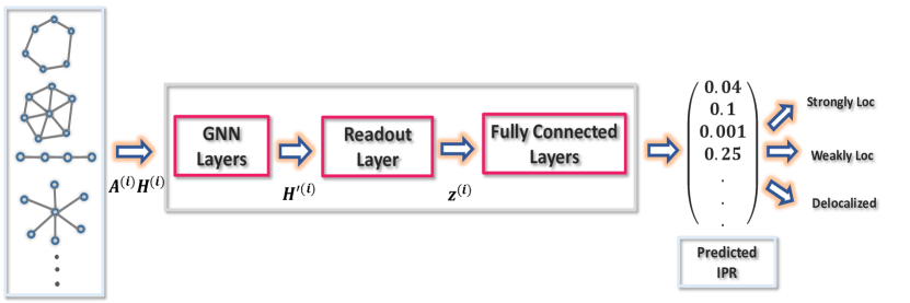
Figure 2: The architecture of the Graph Neural Networks for the regression task over the graphs. The $i^{th}$ input graph (${\bf A}^{(i)}$) and the associated node features (${\bf H}^{(i)}$) are given in matrix form to the models. The Graph Neural Network (GNN) layers of the model output updated node feature matrix (${\bf H}^{{}^{\prime}(i)}$), and the readout layer gives graph level representation as $\bm{z}^{(i)}$. Further, a fully connected layer predicts the IPR value. Finally, we apply a threshold scheme (Eq. (10)) to identify different linear dynamical states.

We quantify the (de)localization behavior of the steady-state ($\bm{x}^{*}$) or the PEV ($\bm{u}\equiv\bm{u}_{1}^{\bf A}$) using the inverse participation ratio ($y_{\bm{x}^{*}}$), which is the sum of the fourth power of the state vector entries and calculate as [20]

$$y_{\bm{x}^{*}}=\frac{\sum_{i=1}^{n}{x^{*}_{i}}^{4}}{\biggl{[}\sum_{i=1}^{n}{x^{*}_{i}}^{2}\biggr{]}^{2}}$$ (6)

where $x^{*}_{i}$ is the $i^{\text{th}}$ component of $\bm{x^{*}}=(x^{*}_{1},x^{*}_{2},\dots,x^{*}_{n})^{T}$ and $\sum_{i=1}^{n}{x^{*}_{i}}^{2}$ is the normalization term. A vector with component $(c,c,\ldots,c)$ is delocalized and has $y_{\bm{x}^{*}}=\frac{1}{n}$ for some positive constant $c>0$, whereas the vector with components $(1,0,\ldots,0)$ yields $y_{\bm{x}^{*}}=1$ and referred as most localized. Furthermore, we consider the networks to be simple, connected and undirected. Hence, some information can easily propagate from one node to another and we never get a steady-state vector of the form $\bm{x}^{*}=(1,0,\ldots,0)$ for a connected network, and thus the IPR value lies between $\frac{1}{n}\leq y_{\bm{x}^{*}}<1$. Therefore, the localization-delocalization behavior of the linear dynamics in the network is quantified using a real value, i.e., each graph associates an IPR value [21, 20, 8, 11]. Now, to identify the states ($\bm{x}^{*}$) belong to which category of dynamical behavior for linear dynamics, we formalize a threshold scheme for identifying IPR values ($y\equiv y_{\bm{x}^{*}}$) lies in the range $[1/n,1)$. We define two thresholds, $\tau_{1}$ and $\tau_{2}$, such that $1/n\leq\tau_{1}<\tau_{2}<1$. An additional parameter $\epsilon$ ($\epsilon>0$) defines some flexibility around the thresholds.

Delocalized region ($r_{1}$). IPR values significantly below the first threshold, including an $\epsilon$-width around $\tau_{1}$:

$$r_{1}=\{y\in[1/n,1)\mid y\leq\tau_{1}-\epsilon\}$$ (7)

Weakly localized region ($r_{2}$). IPR values around and between the two thresholds, including $\epsilon$-width around $\tau_{1}$ and $\tau_{2}$:

$$r_{2}=\{y\in[1/n,1)\mid\tau_{1}-\epsilon<y<\tau_{2}+\epsilon\}$$ (8)

Strongly localized region ($r_{3}$). IPR values significantly above the second threshold, including an $\epsilon$-width around $\tau_{2}$:

$$r_{3}=\{y\in[1/n,1)\mid y\geq\tau_{2}+\epsilon\}$$ (9)

The regions can be defined using a piece-wise function:

$$r(y,\tau_{1},\tau_{2},\epsilon)=\begin{cases}1&\text{if }y\leq\tau_{1}-\epsilon\\ 2&\text{if }\tau_{1}-\epsilon<y<\tau_{2}+\epsilon\\ 3&\text{if }y\geq\tau_{2}+\epsilon\\ \end{cases}$$ (10)

For instance, we consider a set of threshold values as $\tau_{1}=0.05$, $\tau_{2}=0.2$, $\epsilon=1e-6$. Now, if we consider a regular network (each node have the same degree) of $n$ nodes, we have PEV, $\bm{u}^{\mathcal{R}}=(\frac{1}{\sqrt{n}},\frac{1}{\sqrt{n}},\ldots,\frac{1}{\sqrt{n}})$ of A (Theorem 6 [22]) yielding, $y_{\bm{u}^{\mathcal{R}}}=\frac{1}{n}$, thus $y_{\bm{u}^{\mathcal{R}}}\rightarrow 0$ as $n\rightarrow\infty$. On the other hand, for a star graph having $n$ nodes, $\bm{u}^{\mathcal{S}}=\biggl{(}\frac{1}{\sqrt{2}},\frac{1}{\sqrt{2(n-1)}},\ldots,\frac{1}{\sqrt{2(n-1)}}\biggr{)}$ and, $y_{\bm{u}^{\mathcal{S}}}=\frac{1}{4}+\frac{1}{4(n-1)}$. Hence, for $n\rightarrow\infty$, we get $y_{\bm{u}^{\mathcal{S}}}\approx 0.25$, and PEV is strongly localized for the star networks. Further, it is also difficult to find a closed functional form of PEV for any network, and thereby, it is hard to find the IPR value analytically. For instance, in Erdös-Rényi (ER) random networks, we get a delocalized PEV due to each node having the same expected degree [23]. In contrast, the presence of power-law degree distribution for SF networks leads to some localization in the PEV. For SF networks, the IPR value, while being larger than the ER random networks, is much lesser than the star networks [24]. It may seem that when the network structure is close to regular, linear dynamics are delocalized, and increasing degree heterogeneity increases the localization. However, always looking at the degree heterogeneity not able to decide localization and analyzing structural and spectral properties is essential [20, 11]. A fundamental question at the core of the structural-dynamical relation is: Can we predict the steady state behavior of a linear dynamical process in complex networks?

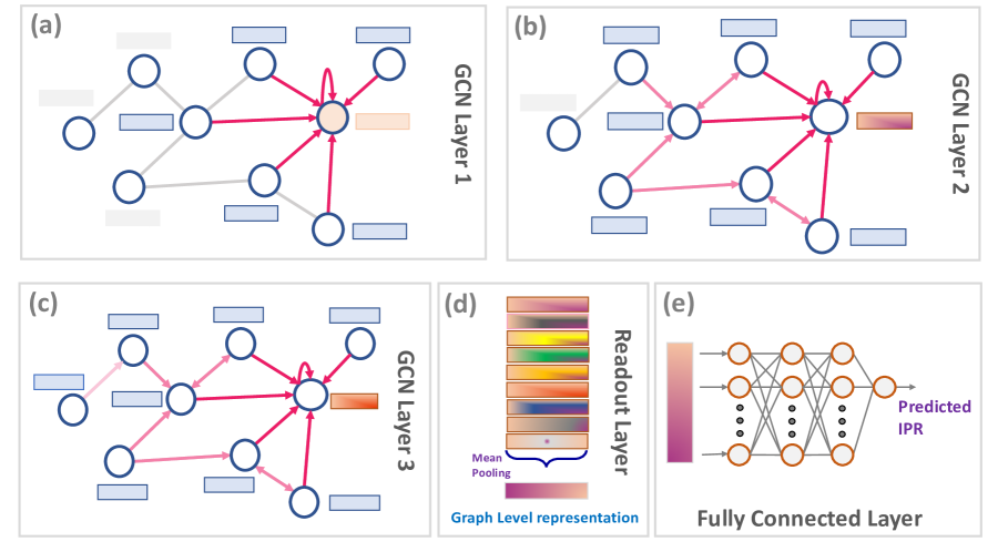
Figure 3: Neural message passing in Graph Convolutional Networks (GCN) model for the regression task. Each node’s features are represented with a small rectangle associated with the node. (a) represents one layer of GCN where a node aggregates and updates its feature based on the immediate neighbor and its features. (b) For the second GCN layer, a node updates its features by aggregating the messages from neighbors to neighbors and its own. (c) The third layer of GCN aggregates the messages from neighbors to neighbors to neighbors. (d) The readout layer creates a graph-level representation from all node features through the mean pooling function that holds the graph’s global information based on the neural message passing framework. (e) Finally, we pass it to a fully connected neural network for the graph’s IPR value prediction task.

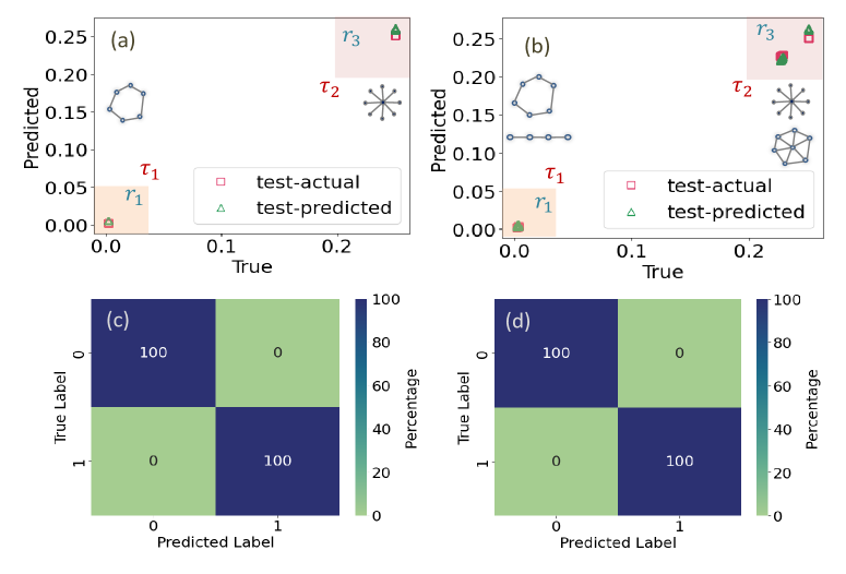
Figure 4: We train the GCN model with two types of structures associated with delocalized and strongly localized states. The input to the GCN model is the cycle and star graphs and the associated target values, i.e., IPR. (a) We give datasets with varying-sized cycle and star networks during the test time. We can observe the true and predicted IPR values. Finally, we apply the threshold function (Eq. (10)) on the predicted IPR value. For our study, we choose the parameters for the threshold values as $\tau_{1}=0.05$, $\tau_{2}=0.2$, and $\epsilon=1e-6$ in Eq. (10). We mark the delocalized region ($r_{1}$) with an orange color box and the strongly localized region ($r_{3}$) with a red color box based on $\tau_{1}$ and $\tau_{2}$ values. This visualization enables us to identify the test network as delocalized and strongly localized based on their predicted IPR values. If predicted IPR values fall within the designated region, the identification of steady-state behavior prediction is correct. Notably, the threshold scheme also allows us to identify the correct behavior even when predicted IPR values deviate from the original values but lie within the threshold boundary. (b) To observe the expressivity of the model, we incorporate two other different network structures (wheel and path networks) and repeat the process. (c, d) We can observe the model-predicted values with high accuracy in the confusion matrix (in $\%$).

Here, we formulate the problem as a graph regression task to predict a target value, IPR, associated with each graph structure. For a given set of graphs $\{\mathcal{G}_{i}\}_{i=1}^{N}$ where each $\mathcal{G}_{i}=(V_{i},E_{i})$ consists of a set of nodes $V_{i}$ and a set of edges $E_{i}$ such that $n_{i}=|V_{i}|$ and $m_{i}=|E_{i}|$. We represent each $\mathcal{G}_{i}$ using its adjacency matrix ${\bf A}^{(i)}$. Further, each graph $\mathcal{G}_{i}$ has an associated target value, i.e., IPR value, $y^{(i)}\in\mathbb{R}$. For each node $v\in V_{i}$ in $\mathcal{G}_{i}$, there is an associated feature vector $\bm{h}_{j}^{(i)}\in\mathbb{R}^{d}$ and $\mathbf{H}^{(i)}\in\mathbb{R}^{|V_{i}|\times d}$ be the node feature matrix where $\bm{h}_{j}^{(i)}$ is the $j^{th}$ row. The objective is to learn a function $f:\mathcal{G}\to\mathbb{R}$, such that $f(\mathcal{G}_{i})\approx y^{(i)}$ for the given set of $N$ graphs.

III Methodology and Results

The function $f$ can be parameterized by a model, in our case, Graph Convolutional Networks (GCN) and Graph Attention Networks (GAT) (Appendix B, C). Let $\bm{\theta}$ be the parameters of the model. The prediction for $\mathcal{G}_{i}$ is denoted by $\hat{y}^{(i)}=f(\mathcal{G}_{i};\bm{\theta})$. The model parameters $\bm{\theta}$ are learned by minimizing a loss function that measures the difference between the predicted values $\hat{y}^{(i)}$ and the true target values $y^{(i)}$. We use the Mean Squared Error (MSE) loss function as

$$\mathcal{L}(\bm{\theta})=\frac{1}{N}\sum_{i=1}^{N}(\hat{y}^{(i)}-y^{(i)})^{2}$$ (11)

Hence, the graph regression problem can be formalized as finding the optimal parameters $\bm{\theta}$ of a model $f$ that minimize the loss function $\mathcal{L}(\bm{\theta})$, enabling the prediction of IPR values for given graphs.

III.1 GCN Architecture

The GCN architecture comprises three graph convolutional layers, each followed by a ReLU activation function. After that, a readout layer performs mean pooling to aggregate node features into a single graph representation. Finally, we use a fully connected layer that outputs the scalar IPR value for the regression task (Fig. 2). A brief description of the architecture is provided below.

Input Layer: The input layer recieves a normalized adjacency ($\hat{\mathbf{A}}$) and initial node feature ${\bf H}^{(0)}$ matrices.

Graph Convolution Layers: We stack three graph convolution layers (Eq. 12) to capture local and higher-order neighborhood information of a node. After each graph convolution layer, we apply nonlinear activation functions (ReLU). Each layer uses the node representations from the previous layer to compute updated representations in the current layer. The first layer of GCN facilitates information flow between first-order neighbors (Fig. 3(a)), while the second layer aggregates information from the second-order neighbors, i.e., the neighbors of a node’s neighbors (Fig. 3(b)), and this process continues for subsequent layers (Fig. 3(c)) and we get

$$\mathbf{H}^{(l)}=\sigma\big{(}\hat{\mathbf{A}}{\bf H}^{(l-1)}\mathbf{W}^{(l-1)}\big{)},\;l=\{1,2,3\}$$ (12)

where ${\bf H}^{(0)}\in\mathbb{R}^{n\times d}$ is the initial input feature matrix, and $\mathbf{W}^{(0)}\in\mathbb{R}^{d\times k_{0}},\mathbf{W}^{(1)}\in\mathbb{R}^{k_{0}\times k_{1}},\mathbf{W}^{(2)}\in\mathbb{R}^{k_{1}\times k_{2}}$ are the weight matrices for the first, second, and third layers, respectively. Hence, ${\bf H}^{(1)}\in\mathbb{R}^{n\times k_{0}}$, and ${\bf H}^{(2)}\in\mathbb{R}^{n\times k_{1}}$ are the intermediate node features matrices and after three layers of graph convolution, final output node features are represented as $\mathbf{H}^{(3)}\in\mathbb{R}^{n\times k_{2}}$.

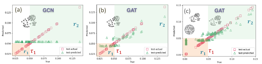
Figure 5: We use scale-free networks for training and testing. (a) We can observe very low accuracy during the test time for the GCN model. (b) However, we can observe increased accuracy using the Graph Attention Network. (c) We consider ER random and scale-free networks and associated IPR values leading to the dynamical states being delocalized and weakly localized. We can observe the GAT model predicts the state’s IPR value with significant accuracy. Here, we train the model for $500$ epochs.

Readout Layer: For the scalar value regression task over a set of graphs, we incorporate a readout layer to aggregate all node features into a single graph-level representation (Fig. 3(d)). We use mean pooling as a readout function,

$$\bm{z}=\texttt{READOUT}(\mathbf{H}^{(3)})=\frac{1}{n}\sum_{j=1}^{n}\bm{h}^{(3)}_{j}$$ (13)

where $\bm{h}^{(3)}_{j}\in\mathbb{R}^{1\times k_{2}}$ is the $j^{th}$ row of ${\bf H}^{(3)}\in\mathbb{R}^{n\times k_{2}}$ and $\bm{z}\in\mathbb{R}^{k_{2}}$. Finally, we pass it to a linear part of the basic neural network (Fig. 3(e)) to perform regression task over graphs and output the predicted IPR value as

$$\hat{y}=\bm{z}\mathbf{W}^{\text{(lin)}}+b$$ (14)

where $\mathbf{W}^{\text{(lin)}}\in\mathbb{R}^{k_{2}\times 1}$ is the weight matrix and $b\in\mathbb{R}$ is the bias value. For our architecture, $\bm{\theta}=\{\mathbf{W}^{(0)},\mathbf{W}^{(1)},\mathbf{W}^{(2)},\mathbf{W}^{\text{(lin)}},b\}$. After getting the predicted IPR value, we use the threshold scheme (Eq. 10) to identify the steady state behavior on complex networks.

III.2 Data Sets Preparation

For the regression task, we create the graph data sets by combining delocalized, weakly localized, and strongly localized network structures, which include star, wheel, path, cycle, and random graph models as Erdős-Rényi (ER) and the Scale-free (SF) networks (Appendix D). As predictions of the GNN model are independent of network size, we vary the size of the networks during dataset creation and store them as edge lists (${\bf A}^{(i)}$). For each network, we calculate the IPR value from the principal eigenvector (PEV) and assign it as the target value ($y^{(i)}$) to $\mathcal{G}_{i}$ in the datasets. Since we do not have predefined node features for the networks, and the GCN framework requires node features as input [25], we initialize the feature vector ($\bm{h}_{j}^{(i)}$) for each node with network-specific properties (clustering coefficient, PageRank, degree centrality, betweenness centrality and closeness centrality) to form the initial feature matrix (${\bf H}^{(0,i)}$) for the $i$th graph. However, the feature matrix could also be initialized with random binary values (i.e., $0$, $1$) [25]. We pass the edge indices, feature matrices, and labels into the model for the regression task, $\{({\bf A}^{(i)},{\bf H}^{(0,i)},y^{(i)})\}_{i=1}^{N}$. We primarily use small-sized networks for training the model, while testing is conducted on networks ranging from small to large sizes, including sizes similar to and beyond those used in training.

We also consider real-world benchmark datasets (ENZYMES, $\texttt{NCI}1$ and $\texttt{MCF}-7$) to train the model [26, 27]. ENZYMES is a dataset of $\texttt{N}_{\texttt{ENZ}}=600$ protein tertiary structures obtained from the BRENDA enzyme database. The $\texttt{NCI}1$ graph dataset is a benchmark dataset used in cheminformatics, where each graph represents a chemical compound, with nodes representing atoms and edges representing bonds between them. The $\texttt{NCI}1$ contains $\texttt{N}_{\texttt{NCI}}=4110$ graphs, and each node has $37$ features. The $\texttt{MCF}-7$ dataset consists of small molecule activities against breast cancer tumors of $\texttt{N}_{\texttt{MCF}}=27770$ graphs where each node has $46$ features.

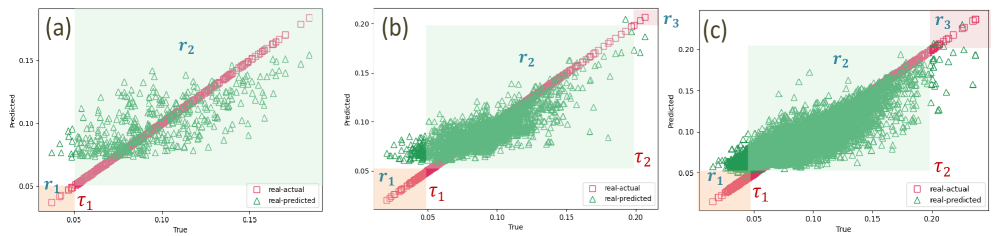
Figure 6: Prediction of Graph Attention Networks (GAT) on real world data sets (ENZYMES, $\texttt{NCI}1$ and $\texttt{MCF}-7$) [26, 27]. (a-c) Our model can also predict the IPR value during testing for real-world graph data sets. We can observe the GAT model predicts the state’s IPR value with significant accuracy. (b) We train the model for $200$ epochs for the real-world dataset. We choose $\tau_{1}=0.05$, $\tau_{2}=0.2$, $\epsilon=1e-6$.

We access the datasets through PyTorch Geometric libraries and preprocess the data sets by removing all the disconnected graphs and those with fewer than $10$ nodes. We incorporate node features extracted from network properties. The sizes of our preprocessed datasets are $\texttt{N}_{\texttt{ENZ}}=441$, $\texttt{N}_{\texttt{NCI}}=2796$, and $\texttt{N}_{\texttt{MCF}}=25084$ with each nodes having seven features as in the model network. Note that IPR values for disconnected graphs are trivially high, and we focus exclusively on connected graphs in our study. For real-world data sets, we divide $80\%$ of the data for training and the rest for testing.

III.3 Training and Testing Strategy

During the training, the GCN model initializes the model parameters ($\bm{\theta}$). We initialize ${\bf W}^{(l-1)}$ at random using the initialization described in Glorot & Bengio (2010) [28]. During the forward pass, for each graph $\mathcal{G}_{i}$, we compute the graph representation using the GCN layers, which involves message passing and aggregation of node features (Fig. (3)). Finally, the model predicts the target value $\hat{y}^{(i)}$. Further, the model computes the loss $\mathcal{L}(\bm{\theta})$ using the predicted ($\hat{y}^{(i)}$) and true target ($y^{(i)}$) values. During the backward pass, the model computes the gradients of the loss with respect to the model parameters. In the next step, the model updates the parameters using an optimization algorithm such as Adam with a learning rate of $0.01$ and a weight decay of $5e-4$. We repeat the forward propagation, loss computation, backward propagation, and parameter update steps until convergence. For our experiment, we choose $d=7$ features for each node and weight matrix sizes as $k_{0}=k_{1}=k_{2}=64$ in different layers.

We start by creating a simple experimental setup where the input dataset contains only two different types of model networks. One type of network (cycle) is associated with delocalized steady-state behavior, and another (star) is in the strongly localized behavior. During the training phase, we send the edge list (${\bf A}^{(i)}$), node feature matrix (${\bf H}^{(0,i)}$), and IPR values ($y^{(i)}$) associated with the graphs as labels for the regression task. Once the model is trained, one can observe that the GCN model accurately predicts the IPR value for the two different types of networks (Fig. 4(a)). More importantly, we train the model with smaller-size networks ($n_{i}=200$ to $300$) and test it with large-size networks ($n_{i}=400$ to $500$) and training datasets contains $N_{train}=1000$ networks and testing datasets size as $N_{test}=500$. Thus, the training cost would be less, and it can easily handle large networks. Furthermore, for the expressivity of the model, we increase the datasets by incorporating two more different types of graphs (path and wheel graphs), where one is delocalized and the other is in strongly localized structures, and we trained the model. We repeat the process by sending the datasets for the regression task to our model and observing that the model provides good accuracy for the test data sets (Fig. 4(b)). Finally, we apply the threshold function (Eq. 10) on the predicted values and achieve very high accuracy in identifying the dynamic state during the testing (Fig. 4(c, d)). One can observe that the GCN model learns the IPR value well for the above network structures.

We move further and incorporate random graph structures (ER and scale-free random networks) in the data sets. Note that the ER random graph belongs to the delocalized state, and SF belongs to both the delocalized and weakly localized state. We train the model with only the SF networks, and during the testing time, one can observe accuracy is not good (Fig. 5(a)). To resolve this, we changed the model and the parameters. We choose the Graph Attention network [29], update the loss function by considering the $\log$ value, and choose AdamW optimizer instead of Adam. We also use a dropout rate of $0.6$ and set learning rare to $1e-5$ in the model. The new setup leads to improvement in the results (Fig. 5(b)). Now, we consider both ER and SF networks and train the model, and during the testing time, we can observe good accuracy in predicting the IPR values (Fig. 5(c)).

The performance of GCN and GAT in identifying various dynamic states in model networks is highly accurate. GCN is particularly effective in distinguishing between strongly localized and delocalized states (Fig. 4), while GAT excels at differentiating weakly localized and delocalized states (Fig. 5(c)). Although trained models reliably predict states in model networks, applying them to real-world data presents challenges due to imbalanced state distribution and limited dataset size in the $r_{1}$ and $r_{3}$ regions (Fig. 6). To assess real-world applicability, we trained the GAT model on real-world data sets and achieved reasonable accuracy on test datasets (Fig. 6(a-c)).

III.4 Insights of Training Process

To understand the explainability of our model, we provide mathematical insights into the training process via forward and backward propagation to predict the IPR value. Our derivation offers an understanding of the updation of weight matrices. We perform the analysis with a single GCN layer, a readout layer, and a linear layer for simplicity. However, our framework can easily be extended to more layers.

Forward Propagation:

GCN Layer: ${\bf H}^{(1,i)}=\sigma(\hat{\bf A}^{(i)}{\bf H}^{(0,i)}{\bf W})$

Readout Layer: $\bm{z}^{(i)}=\frac{1}{n_{i}}\sum_{j=1}^{n_{i}}\bm{h}^{(1,i)}_{j}$

Linear Layer: $\hat{y}^{(i)}=\bm{z}^{(i)}{\bf W}^{(\text{lin})}+b$

Loss function: $\mathcal{L}=\frac{1}{N}\sum_{i=1}^{N}(y^{(i)}-\hat{y}^{(i)})^{2}$

In the above, $\hat{\bf A}^{(i)}$ is the normalized adjacency matrix, ${\bf H}^{(0,i)}$ is the initial feature matrix, and W is the learnable weight matrix. Further, $\bm{h}^{(1,i)}_{j}=\sigma\biggl{(}\sum_{k=1}^{n_{i}}\hat{A}^{(i)}_{jk}\bm{h}^{(0,i)}_{k}{\bf W}\biggr{)}$ is the feature vector of node $j$ in graph $i$ and $j^{th}$ row of updated feature matrix ${\bf H}^{(1,i)}$ (Example 1). Further, ${\bf W}^{(\text{lin})}$ and $b$ are the learnable weights of the linear layer. Finally, $y^{(i)}$ is the true scalar value for $\mathcal{G}_{i}$ and $\hat{y}^{(i)}$ is the predicted IPR value.

Backward Propagation: To compute the gradients to update the weight matrices, we apply the chain rule to propagate the error from the output layer back through the network layers. We calculate the gradient of loss with respect to the output of the linear layer as

$$\frac{\partial\mathcal{L}}{\partial\hat{y}^{(i)}}=\frac{2}{N}(\hat{y}^{(i)}-y^{(i)})$$ (15)

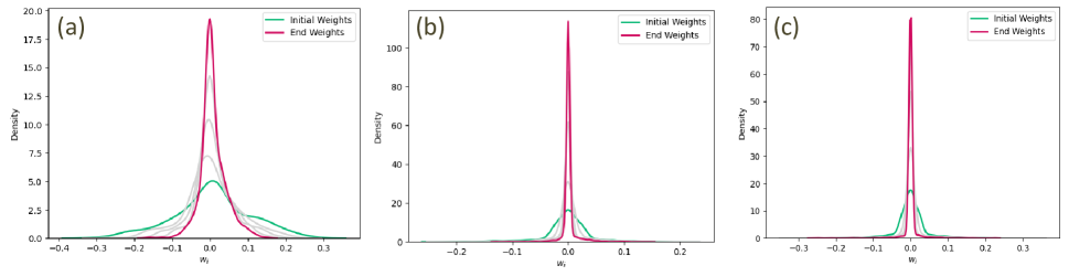
Figure 7: Portray the distribution of weight matrices ($\mathbf{W}^{(0)},\mathbf{W}^{(1)},\mathbf{W}^{(2)}$) entries for the three GCN layers during the training process with cycle and star networks (Fig. 4(a)). We show the weights matrix entries for the first five epochs, where the ‘Initial Weights’ infer the initial weight matrix, and the ‘End Weights’ infer the weight matrix after the fourth epochs. The gray color indicated weight matrices during epochs $1$, $2$, and $3$.

We calculate the gradients for the linear layer. We know that each graph $i$ contributes to the overall loss $\mathcal{L}$. Therefore, we accumulate the gradient contributions from each graph when computing the gradient of the loss with respect to the weight matrix ${\bf W}^{(\text{lin})}$ (Example 2). Thus, to obtain the gradient of the loss with respect to the weights ${\bf W}^{(\text{lin})}$, we apply the chain rule

$$\frac{\partial\mathcal{L}}{\partial{\bf W}^{(\text{lin})}}=\sum_{i=1}^{N}\biggl{(}\frac{\partial\mathcal{L}}{\partial\hat{y}^{(i)}}\cdot\frac{\partial\hat{y}^{(i)}}{\partial{\bf W}^{(\text{lin})}}\biggr{)}=\sum_{i=1}^{N}\frac{2}{N}(\hat{y}^{(i)}-y^{(i)})z^{(i)}$$ (16)

where $\frac{\partial\hat{y}^{(i)}}{\partial{\bf W}^{(\text{lin})}}=z^{(i)}$. Similarly, we calculate the gradient with respect to $b$ and $z^{(i)}$ as

$$\begin{split}\frac{\partial\mathcal{L}}{\partial b}&=\sum_{i=1}^{N}\biggl{(}\frac{\partial\mathcal{L}}{\partial\hat{y}^{(i)}}\cdot\frac{\partial\hat{y}^{(i)}}{\partial b}\biggr{)}=\sum_{i=1}^{N}\frac{2}{N}(\hat{y}^{(i)}-y^{(i)})\\ \frac{\partial\mathcal{L}}{\partial z^{(i)}}&=\frac{\partial\mathcal{L}}{\partial\hat{y}^{(i)}}\cdot\frac{\partial\hat{y}^{(i)}}{\partial\bm{z}^{(i)}}=\frac{2}{N}(\hat{y}^{(i)}-y^{(i)}){\bf W}^{(\text{lin})}\end{split}$$ (17)

Now, we calculate the gradient for the Readout layer as

$$\frac{\partial\mathcal{L}}{\partial\bm{h}^{(1,i)}_{j}}=\frac{\partial\mathcal{L}}{\partial\bm{z}^{(i)}}\cdot\frac{\partial\bm{z}^{(i)}}{\partial\bm{h}^{(1,i)}_{j}}=\frac{2}{N}(\hat{y}^{(i)}-y^{(i)}){\bf W}^{(\text{lin})}\cdot\frac{1}{n_{i}}$$ (18)

where $\bm{z}^{(i)}=\frac{1}{n_{i}}\sum_{j=1}^{n_{i}}\bm{h}^{(1,i)}_{j}$ and thus $\frac{\partial\bm{z}^{(i)}}{\partial\bm{h}^{(1,i)}_{j}}=\frac{1}{n_{i}}$. Finally, we calculate the gradients for the GCN Layer. We have $N$ different graphs in our dataset, and each $\mathcal{G}_{i}$ has $n_{i}$ nodes. The total gradient with respect to ${\bf W}$ accumulates the contributions from all nodes in all graphs. Hence, we sum over all nodes in each graph and then over all graphs as

$$\frac{\partial\mathcal{L}}{\partial{\bf W}}=\sum_{i=1}^{N}\sum_{j=1}^{n_{i}}\biggl{(}\frac{\partial\mathcal{L}}{\partial\bm{h}^{(1,i)}_{j}}\cdot\frac{\partial\bm{h}^{(1,i)}_{j}}{\partial{\bf W}}\biggr{)}$$ (19)

We know the layer output for the $i^{th}$ graph as ${\bf H}^{(1,i)}=\sigma(\hat{\bf A}^{(i)}{\bf H}^{(0,i)}{\bf W})$. Hence, for a single node $j$ in graph $i$, its node representation after the GCN layer is

$$\bm{h}^{(1,i)}_{j}=\sigma\left(\sum_{k=1}^{n_{i}}\hat{A}^{(i)}_{jk}\bm{h}^{(0,i)}_{k}{\bf W}\right)=\sigma(\bm{q}^{(i)}_{j})$$ (20)

where $\bm{q}^{(i)}_{j}=\sum_{k=1}^{n_{i}}\hat{A}^{(i)}_{jk}\bm{h}^{(0,i)}_{k}{\bf W}$ and $\hat{A}^{(i)}_{jk}$ is the element in the $j^{th}$ row and $k^{th}$ column of the normalized adjacency matrix, representing the connection between node $j$ and node $k$ and $\bm{h}^{(0,i)}_{k}$ refers to the $k^{th}$ row of the input feature matrix ${\bf H}^{(0,i)}$ of graph $i$. To compute $\frac{\partial\bm{h}^{(1,i)}_{j}}{\partial{\bf W}}$, we apply the chain rule as

$$\frac{\partial\bm{h}^{(1,i)}_{j}}{\partial{\bf W}}=\frac{\partial\bm{h}^{(1,i)}_{j}}{\partial\bm{q}^{(i)}_{j}}\cdot\frac{\partial\bm{q}^{(i)}_{j}}{\partial{\bf W}}$$ (21)

We can calculate the partial derivative with respect to $\bm{q}^{(i)}_{j}$ as

$$\frac{\partial\bm{h}^{(1,i)}_{j}}{\partial\bm{q}^{(i)}_{j}}=\sigma^{\prime}\left(\bm{q}^{(i)}_{j}\right)$$ (22)

where, $\sigma^{\prime}(\bm{q}^{(i)}_{j})$ is the derivative of $\sigma$. Now the partial derivative of $\bm{q}^{(i)}_{j}$ with respect to ${\bf W}$ as

$$\frac{\partial\bm{q}^{(i)}_{j}}{\partial{\bf W}}=\sum_{k=1}^{n_{i}}\hat{A}^{(i)}_{jk}\bm{h}^{(0,i)}_{k}$$ (23)

We can observe that $\bm{q}^{(i)}_{j}$ is a linear combination of the rows of ${\bf H}^{(0,i)}$ weighted by $\hat{\bf A}^{(i)}_{j}$. In matrix notation, we can write as

$$\frac{\partial\bm{q}^{(i)}_{j}}{\partial{\bf W}}=\hat{A}^{(i)}_{j}{\bf H}^{(0,i)}$$ (24)

where $\hat{A}^{(i)}_{j}$ is the $j^{th}$ row of ${\bf\hat{A}}^{(i)}$. Now, we combine the results of the chain rule and get

$$\frac{\partial\bm{h}^{(1,i)}_{j}}{\partial{\bf W}}=\sigma^{\prime}\left(\bm{q}^{(i)}_{j}\right)\cdot\hat{A}^{(i)}_{j}{\bf H}^{(0,i)}$$ (25)

In Eq. (19), we substitute Eqs. (18) and (25) and get

$$\begin{split}\frac{\partial\mathcal{L}}{\partial{\bf W}}&=\frac{2}{N}\sum_{i=1}^{N}\sum_{j=1}^{n_{i}}(\hat{y}^{(i)}-y^{(i)}){\bf W}^{(\text{lin})}\cdot\frac{1}{n_{i}}\cdot\sigma^{\prime}(\bm{q}^{(i)}_{j})\\ &\cdot(\hat{A}^{(i)}_{j}{\bf H}^{(0,i)})\end{split}$$ (26)

where $\bm{q}^{(i)}_{j}=\sum_{k=1}^{n_{i}}\hat{A}^{(i)}_{jk}\bm{h}^{(0,i)}_{k}{\bf W}$. Finally, the weight matrices are updated using gradient descent as

$$\begin{split}{\bf W}&\leftarrow{\bf W}-\eta\frac{\partial\mathcal{L}}{\partial{\bf W}}\\ {\bf W}^{(\text{lin})}&\leftarrow{\bf W}^{(\text{lin})}-\eta\frac{\partial\mathcal{L}}{\partial{\bf W}^{(\text{lin})}}\\ b&\leftarrow b-\eta\frac{\partial\mathcal{L}}{\partial b}\end{split}$$ (27)

where $\eta$ is the learning rate. The above process is repeated iteratively: forward propagation $\rightarrow$ loss calculation $\rightarrow$ backward propagation $\rightarrow$ weight update until the model converges to an optimal set of weights that minimize the loss. For simplicity in backward propagation analysis, we use gradient-based optimization. However, all numerical results are reported using the Adam/AdamW optimization scheme. Recent research on backward propagation in GCN for node classification and link prediction can be found in [30].

We observe the weight matrices of different layers during the training time. The distribution of the weight matrices provides a visual representation of the weights learned during the training process (Fig. 7). The magnitude of each weight indicates the importance of the corresponding feature. The higher absolute values in the weight matrices suggest that the feature significantly impacts the model’s predictions. We can observe that for different layers, weight matrix values are initially spread evenly around from zeros, but as time progresses, values become close to zeros (Fig. 7).

IV Conclusion

Using the graph neural network, we introduce a framework to predict the localized and delocalized states of complex unknown networks. We focus on leveraging the rich information embedded in network structures and extracting relevant features for graph regression. Specifically, a GCN model is employed to predict inverse participation ratio values for unknown networks and consequently identify localized or delocalized states. Our approach provides a graph neural network alternative to the traditional principal eigenvalue analysis [20] for understanding the behavior of linear dynamical processes in real-world systems at steady state. This method offers near real-time insight into the structural properties of underlying networks. A key advantage of the proposed framework is its ability to train on small networks and generalize to larger networks, achieving an accuracy of nearly $\sim 100\%$ with test unseen model networks to understand delocalized or strongly localized states. This makes the model scale-invariant, with the computational cost of state prediction remaining consistent regardless of network size, apart from the cost of reading the network data.

Our trained GNN framework (e.g., GCN and GAT) effectively identifies three different states in unseen test model network data. Moreover, our model accurately identifies the states in the weakly localized regions for the real-world data. However, distinguishing between delocalized weakly localized and strongly localized states associated with real-world graphs poses a significant challenge. It might be due to the imbalance of data points in different states and limited dataset availability. Moving forward, we aim to address these challenges and improve identification accuracy.

References

V Appendix

V.1 Linear Dynamics

We can write Eq. (1) in matrix form as

$$\frac{d\bm{x(t)}}{dt}={\bf M}\bm{x}(t)$$ (28)

where M is a transition matrix given by ${\bf M}=\alpha{\bf I}+\beta{\bf A}$, where I is the identity matrix. Note that M and A only differ by constant term. Hence,

$$\bm{x}(t)=e^{{\bf M}t}\bm{x}(0)$$ (29)

We consider ${\bf M}\in\mathbb{R}^{n\times n}$ is diagonalizable, ${\bf M}={\bf U\Lambda U^{-1}}$ and ${\bf UU^{-1}}={\bf I}$ where columns of U are the eigenvectors ($\{\bm{u}_{1}^{\bf M},\bm{u}_{2}^{\bf M},\ldots,\bm{u}_{n}^{\bf M}\}$) of M and having $n$ number of distinct eigenvalues $\{\lambda_{1}^{\bf M},\lambda_{2}^{\bf M},\ldots,\lambda_{n}^{\bf M}\}$ which are diagonally stored in $\Lambda$. We know $\bm{x}(0)$ is an arbitrary initial state. Thus, we can represent it as a linear combination of eigenvectors of M, and therefore, we can write Eq. (29).

$$\begin{split}\bm{x}(t)&=e^{{\bf M}t}[c_{1}(0)\bm{u}_{1}^{\bf M}+c_{2}(0)\bm{u}_{2}^{\bf M}+\ldots+c_{n}(0)\bm{u}_{n}^{\bf M}]\\ &={\bf U}e^{{\bf\Lambda}t}{\bf U}^{-1}[c_{1}(0)\bm{u}_{1}^{\bf M}+c_{2}(0)\bm{u}_{2}^{\bf M}+\ldots+c_{n}(0)\bm{u}_{n}^{\bf M}]\\ &={\bf U}e^{{\bf\Lambda}t}{\bf U^{-1}}{\bf U}\bm{c}(0)\\ &={\bf U}e^{{\bf\Lambda}t}\bm{c}(0)\\ &=c_{1}(0)e^{\lambda_{1}^{\bf M}t}\bm{u}_{1}^{\bf M}+c_{2}(0)e^{\lambda_{2}^{\bf M}t}\bm{u}_{2}^{\bf M}+\ldots+c_{n}(0)e^{\lambda_{n}^{\bf M}t}\bm{u}_{n}^{\bf M}\\ &=\sum_{i=1}^{n}c_{i}(0)e^{\lambda_{i}^{\bf M}t}\bm{u}_{i}^{\bf M}\end{split}$$ (30)

such that where $\bm{c}(0)=(c_{1}(0),c_{2}(0),\ldots,c_{n}(0))^{T}$ and

$$\begin{split}e^{{\bf M}t}&={\bf I}+{\bf M}t+\frac{({\bf M}t)^{2}}{2}+\frac{({\bf M}t)^{3}}{3}+\ldots\\ &={\bf I}+{\bf U\Lambda U^{-1}}t+\frac{({\bf U\Lambda U^{-1}}t{\bf U\Lambda U^{-1}}t)}{2!}+\\ &\frac{({\bf U\Lambda U^{-1}}t{\bf U\Lambda U^{-1}}t{\bf U\Lambda U^{-1}}t)}{3!}+\ldots\\ &={\bf U}\biggl{[}{\bf I}+{\bf\Lambda}t+\frac{({\bf\Lambda}t)^{2}}{2!}+\frac{({\bf\Lambda}t)^{3}}{3!}+\ldots\biggr{]}{\bf U^{-1}}\\ &={\bf U}e^{{\bf\Lambda}t}{\bf U^{-1}}\end{split}$$ (31)

For $t\rightarrow\infty$, we can approximate Eq. (30) as

$$\bm{x}^{*}\sim c_{1}(0)e^{\lambda_{1}^{\bf M}t}\bm{u}_{1}^{\bf M}\sim\bm{u}_{1}^{\bf M}$$ (32)

Since the largest eigenvalue $\lambda_{1}$ dominates over the others, the PEV of the adjacency matrix will decide the steady state behavior of the system.

V.2 Mathematical Insights of Graph Convolution Neural Network

Deep Learning models, for example, Convolutional Neural Networks (CNN), require an input of a specific size and cannot handle graphs and other irregularly structured data [31]. Graph Convolution Networks (GCN) are exclusively designed to handle graph-structured data and are preferred over Convolutional Neural Networks (CNN) when dealing with non-Euclidean data. The GCN architecture draws on the same way as CNN but redefines it for the graph domain. Graphs can be considered a generalization of images, with each node representing a pixel connected to eight (or four) other pixels on either side. For images, the graph convolution layer also aims to capture neighborhood information for graph nodes. GCN can handle graphs of various sizes and shapes, which increases its applicability in diverse research domains.

The simplest GNN operators prescribed by Kipf et al. are called GCN [32]. The convolutional layers are used to obtain the aggregate information from a node’s neighbors to update its feature representation. We consider the feature vector as $\bm{h}_{i}^{(l-1)}$ of node $i$ at layer $l-1$ and update the feature vector of node $i$ at layer $l$, as

$$\bm{h}_{i}^{(l)}=\sigma\left(\sum_{j\in\mathcal{N}(i)\cup\{i\}}\frac{1}{\sqrt{\tilde{d}_{i}\tilde{d}_{j}}}\bm{h}_{j}^{(l-1)}\mathbf{W}^{(l-1)}\right)\,,$$ (33)

where new feature vector $\bm{h}_{i}^{(l)}$ for node $i$ has been created as an aggregation of feature vector $\bm{h}_{i}^{(l-1)}$ and the feature vectors of its neighbors $\bm{h}_{j}^{(l-1)}$ of the previous layer, each weighted by the corresponding entry in the normalized adjacency matrix ($\hat{{\bf A}}$), and then transformed by the weight matrix $\mathbf{W}^{(l-1)}$ and passed through the activation function $\sigma$. We use the ReLU activation function for our work.

The sum $\sum_{j\in\mathcal{N}(i)\cup\{i\}}$ aggregates the feature information from the neighboring nodes and the node itself where $\mathcal{N}(i)$ is the set of neighbors of node $i$. The normalization factor $1/\sqrt{\tilde{d}_{i}\tilde{d}_{j}}$ ensures that the feature vectors from neighbors are appropriately scaled based on the node degrees, preventing issues related to scale differences in higher vs. lower degree nodes where $\tilde{d}_{i}$ and $\tilde{d}_{j}$ being the normalized degrees of nodes $i$ and $j$, respectively [33]. The weight matrix $\mathbf{W}^{(l-1)}$ transforms the aggregated feature vectors, allowing the GCN to learn meaningful representations. The activation function $\sigma$ introduces non-linearity, enabling the model to capture complex patterns.

Single convolution layer representation: The operation on a single graph convolution layer can be defined using matrix notation as follows:

$$\begin{split}{\bf H}^{(l)}&=\sigma\left(\hat{{\bf A}}{\bf H}^{(l-1)}{\bf W}^{(l-1)}\right)\\ &=\sigma\left(\tilde{\bf D}^{-\frac{1}{2}}\tilde{{\bf A}}\tilde{\bf D}^{-\frac{1}{2}}{\bf H}^{(l-1)}{\bf W}^{(l-1)}\right)\end{split}$$ (34)

where $\mathbf{H}^{(l-1)}$ is the matrix of node features at layer $l-1$ where $l=1,2,3$, with $\mathbf{H}^{(0)}$ being the input feature matrix. Here, $\tilde{{\bf A}}={\bf A}+{\bf I}$ is the self-looped adjacency matrix by adding the identity matrix I to the adjacency matrix A. After that we do symmetric normalization by inverse square degree matrix with $\tilde{{\bf A}}$ and denoted as $\hat{{\bf A}}=\widetilde{\bf D}^{-\frac{1}{2}}\tilde{{\bf A}}\widetilde{\bf D}^{-\frac{1}{2}}$, where ${\bf D}\in\mathbb{R}^{n\times n}$ is the diagonal degree matrix of ${\bf A}$ with $\tilde{D}_{ii}=\sum_{j=1}^{n}\tilde{A}_{ij}$. Here, ${\bf W}^{(l)}\in\mathbb{R}^{F_{\text{in}}\times F_{\text{out}}}$ is a trainable weight matrix of layer $l$. A linear feature transformation is applied to the node feature matrix by ${\bf HW}$, mapping the $F_{\text{in}}$ feature channels to $F_{\text{out}}$ channels in the next layer. The weights of ${\bf W}$ are shared among all vertices. We use the Glorot (Xavier) initialization that initializes the weights by drawing from a distribution with zero mean and a specific variance [28]. It helps maintain the variance of the activations and gradients through the layers for a weight matrix $\mathbf{W}$

$$\mathbf{W}\sim\mathcal{U}\left(-\sqrt{\frac{6}{F_{\text{in}}+F_{\text{out}}}},\sqrt{\frac{6}{F_{\text{in}}+F_{\text{out}}}}\right)$$ (35)

where, $\mathcal{U}$ denotes the uniform distribution. For the GCN layer implementation, we use GCNConv from the PyTorch Geometric library [34].

V.2.1 Example 1

For instance, we consider matrices

$${\bf A}=\begin{bmatrix}1&2\\ 3&4\end{bmatrix},\quad{\bf H}=\begin{bmatrix}1&0&2\\ -1&3&1\end{bmatrix},\quad{\bf W}=\begin{bmatrix}1&2\\ 0&1\\ -1&0\end{bmatrix}$$

We compute

$${\bf D=AHW}$$

as

$${\bf E=AH}=\begin{bmatrix}1&2\\ 3&4\end{bmatrix}\begin{bmatrix}1&0&2\\ -1&3&1\end{bmatrix}=\begin{bmatrix}-1&6&4\\ -1&12&10\end{bmatrix}$$

Now we compute

$${\bf D=EW}=\begin{bmatrix}-1&6&4\\ -1&12&10\end{bmatrix}\begin{bmatrix}1&2\\ 0&1\\ -1&0\end{bmatrix}=\begin{bmatrix}-5&4\\ -11&10\end{bmatrix}$$

Now, we express the $j$th row of ${\bf D}$ as

$$\bm{d}_{j}=\sum_{k=1}^{n}A_{jk}\bm{h}_{k}{\bf W}$$

For $j=1$ (first row of ${\bf D}$)

$$\bm{d}_{1}=A_{11}\bm{h}_{1}{\bf W}+A_{12}\bm{h}_{2}{\bf W}=(1\bm{h}_{1}+2\bm{h}_{2}){\bf W}$$

We know rows of ${\bf H}$ as

$$\bm{h}_{1}=\begin{bmatrix}1&0&2\end{bmatrix},\quad\bm{h}_{2}=\begin{bmatrix}-1&3&1\end{bmatrix}$$

Hence,

$$1\bm{h}_{1}+2\bm{h}_{2}=\begin{bmatrix}1&0&2\end{bmatrix}+2\times\begin{bmatrix}-1&3&1\end{bmatrix}=\begin{bmatrix}-1&6&4\end{bmatrix}$$

Now, multiplying with ${\bf W}$ we get

$$\bm{d}_{1}=(-1,6,4)\times\begin{bmatrix}1&2\\ 0&1\\ -1&0\end{bmatrix}=\begin{bmatrix}-5&4\end{bmatrix}$$

Similarly, for $j=2$, we get

$$\bm{d}_{2}=(-1,12,10)\times{\bf W}=\begin{bmatrix}-11&10\end{bmatrix}$$

V.2.2 Example 2

Let’s consider an example with three graphs, each having a corresponding $z^{(i)}$ and $y^{(i)}$ as $z^{(1)},z^{(2)},z^{(3)}$ are the outputs from the readout layer and $y^{(1)},y^{(2)},y^{(3)}$ are the true scalar values. If we denote the linear layer weight as ${\bf W}^{(\text{lin})}$, thus we can compute the predictions as

$$\begin{split}\hat{y}^{(1)}&=z^{(1)}{\bf W}^{(\text{lin})}+b\\ \hat{y}^{(2)}&=z^{(2)}{\bf W}^{(\text{lin})}+b\\ \hat{y}^{(3)}&=z^{(3)}{\bf W}^{(\text{lin})}+b\end{split}$$ (36)

Now, we can compute gradients for each graph:

$$\begin{split}\frac{\partial\mathcal{L}}{\partial\hat{y}^{(1)}}&=\frac{2}{3}(\hat{y}^{(1)}-y^{(1)})\\ \frac{\partial\mathcal{L}}{\partial\hat{y}^{(2)}}&=\frac{2}{3}(\hat{y}^{(2)}-y^{(2)})\\ \frac{\partial\mathcal{L}}{\partial\hat{y}^{(3)}}&=\frac{2}{3}(\hat{y}^{(3)}-y^{(3)})\end{split}$$ (37)

Hence, aggregate gradients for ${\bf W}^{(\text{lin})}$ as

$$\begin{split}\frac{\partial\mathcal{L}}{\partial{\bf W}^{(\text{lin})}}&=\left(\frac{2}{3}(\hat{y}^{(1)}-y^{(1)})\right)z^{(1)}+\left(\frac{2}{3}(\hat{y}^{(2)}-y^{(2)})\right)z^{(2)}\\ &+\left(\frac{2}{3}(\hat{y}^{(3)}-y^{(3)})\right)z^{(3)}\end{split}$$ (38)

V.3 Mathematical Insights of Graph Attention Network

Graph Attention Networks (GATs) are an extension of Graph Convolutional Networks (GCNs) that introduce attention mechanisms to improve message passing in graph neural networks [29]. The key advantage of GAT is that it assigns different importance (attention) to different neighbors, making it more flexible and powerful than traditional GCNs, which use fixed aggregation weights.

In a standard GCN, node embeddings are updated by aggregating information from neighboring nodes using fixed weights derived from the adjacency matrix. In a GAT, an attention mechanism is used to dynamically compute different weights for each neighbor, allowing the network to focus more on important neighbors. In GAT, each node feature vector ($\bm{h}_{i}$) is transformed into a higher-dimensional representation using a learnable weight matrix ${\bf W}$ as

$$\bm{h}_{i}^{\prime}={\bf W}\bm{h}_{i}$$ (39)

where ${\bf W}\in\mathbb{R}^{F^{\prime}\times F}$ is a learnable weight matrix, and $F^{\prime}$ is the new feature dimension. Further, for each edge $(i,j)\in E$, compute the attention score $e_{ij}$, which measures the importance of node $j$ ’s features to node $i$. The attention score is calculated as

$$e_{ij}=\text{LeakyReLU}(\mathbf{a}^{T}[{\bf W}\bm{h}_{i}\|{\bf W}\bm{h}_{j}])$$

where $\mathbf{a}\in\mathbb{R}^{2F^{\prime}}$ is a learnable weight vector, $\|$ denotes concatenation, and LeakyReLU is used as a non-linear activation function. Finally, the attention scores are normalized across all neighbors using the softmax function.

$$\alpha_{ij}=\frac{\exp(e_{ij})}{\sum_{k\in\mathcal{N}(i)}\exp(e_{ik})}$$

where $\mathcal{N}(i)$ denotes the neighbors of node $i$. The softmax ensures that the attention weights sum to $1$ for each node. Each node aggregates its neighbors’ transformed features using the learned attention coefficients.

$$\bm{h}_{i}^{\prime}=\sigma\left(\sum_{j\in\mathcal{N}(i)}\alpha_{ij}{\bf W}\bm{h}_{j}\right)$$

where $\sigma$ is a non-linearity (e.g., ReLU). To improve stability, GAT often uses multi-head attention, where multiple attention mechanisms run in parallel, and their outputs are averaged.

$$\bm{h}_{i}^{\prime}=\sigma\left(\frac{1}{K}\sum_{k=1}^{K}\sum_{j\in\mathcal{N}(i)}\alpha_{ij}^{(k)}{\bf W}^{(k)}\mathbf{h}_{j}\right)$$

where $K$ is the number of attention heads, ${\bf W}^{(k)}$ and $\alpha_{ij}^{(k)}$ are the weight matrix and attention coefficients of the $k^{th}$ attention head. For our graph-level IPR value regression task, we use two layers of GAT with four heads for the first layer and one head in the second layer, respectively. For the GAT layer implementation, we use GATConv from the PyTorch Geometric library [34].

V.4 Complex Networks

We prepare the datasets for our experiments using several model networks (cycle, path, star, wheel, ER, and scale-free networks) and their associated IPR values. A few models (ER and scale-free networks) are randomly generated. The ER random network is denoted by $\mathcal{G}^{ER}(n,p)$ where $n$ is the number of nodes and $p$ is the edge probability [35]. The existence of each edge is statistically independent of all other edges. Starting with $n$ number of nodes, connecting them with a probability $p=\langle k\rangle/n$ where $\langle k\rangle$ is the mean degree. The ER random network realization will have a Binomial degree distribution [35]. The SF networks ($\mathcal{G}^{SF}$) generated using the Barabási-Albert model follows a power-law degree distribution [35].

References

- Strogatz [2001] S. H. Strogatz, Exploring complex networks, nature 410, 268 (2001).
- Bassett et al. [2011] D. S. Bassett, N. F. Wymbs, M. A. Porter, P. J. Mucha, J. M. Carlson, and S. T. Grafton, Dynamic reconfiguration of human brain networks during learning, Proceedings of the National Academy of Sciences 108, 7641 (2011).
- Kimble [2008] H. J. Kimble, The quantum internet, Nature 453, 1023 (2008).
- Yang et al. [2022] Z. Yang, F. Liu, Z. Gao, H. Sun, J. Zhao, D. Janssens, and G. Wets, Estimating the influence of disruption on highway networks using gps data, Expert Systems with Applications 187, 115994 (2022).
- Mahapatra et al. [2020] G. Mahapatra, P. Pradhan, R. Chattaraj, and S. Banerjee, Dynamic graph streaming algorithm for digital contact tracing, arXiv preprint arXiv:2007.05637 (2020).
- Filoche and Mayboroda [2012] M. Filoche and S. Mayboroda, Universal mechanism for anderson and weak localization, Proceedings of the National Academy of Sciences 109, 14761 (2012).
- Elsner et al. [1999] U. Elsner, V. Mehrmann, F. Milde, R. A. Römer, and M. Schreiber, The anderson model of localization: a challenge for modern eigenvalue methods, SIAM Journal on Scientific Computing 20, 2089 (1999).
- Pradhan et al. [2020] P. Pradhan, C. Angeliya, and S. Jalan, Principal eigenvector localization and centrality in networks: Revisited, Physica A: Statistical Mechanics and its Applications 554, 124169 (2020).
- Zhang [2016] P. Zhang, Robust spectral detection of global structures in the data by learning a regularization, Advances in Neural Information Processing Systems 29 (2016).
- Gleich and Mahoney [2015] D. F. Gleich and M. W. Mahoney, Using local spectral methods to robustify graph-based learning algorithms, in Proceedings of the 21th ACM SIGKDD International Conference on Knowledge Discovery and Data Mining (2015) pp. 359–368.
- Pradhan and Jalan [2020] P. Pradhan and S. Jalan, From spectra to localized networks: A reverse engineering approach, IEEE Transactions on Network Science and Engineering 7, 3008 (2020).
- Vespignani [2012] A. Vespignani, Modelling dynamical processes in complex socio-technical systems, Nature physics 8, 32 (2012).
- Eubank et al. [2004] S. Eubank, H. Guclu, V. Anil Kumar, M. V. Marathe, A. Srinivasan, Z. Toroczkai, and N. Wang, Modelling disease outbreaks in realistic urban social networks, Nature 429, 180 (2004).
- Longini Jr et al. [2005] I. M. Longini Jr, A. Nizam, S. Xu, K. Ungchusak, W. Hanshaoworakul, D. A. Cummings, and M. E. Halloran, Containing pandemic influenza at the source, Science 309, 1083 (2005).
- Tian et al. [2018] H. Tian, S. Hu, B. Cazelles, G. Chowell, L. Gao, M. Laine, Y. Li, H. Yang, Y. Li, Q. Yang, et al., Urbanization prolongs hantavirus epidemics in cities, Proceedings of the National Academy of Sciences 115, 4707 (2018).
- Dalziel et al. [2018] B. D. Dalziel, S. Kissler, J. R. Gog, C. Viboud, O. N. Bjørnstad, C. J. E. Metcalf, and B. T. Grenfell, Urbanization and humidity shape the intensity of influenza epidemics in us cities, Science 362, 75 (2018).
- Jalan and Pradhan [2020] S. Jalan and P. Pradhan, Wheel graph strategy for pev localization of networks, Europhysics Letters 129, 46002 (2020).
- Strogatz [2018] S. H. Strogatz, Nonlinear dynamics and chaos: with applications to physics, biology, chemistry, and engineering (CRC press, 2018).
- Aguirre et al. [2013] J. Aguirre, D. Papo, and J. M. Buldú, Successful strategies for competing networks, Nature Physics 9, 230 (2013).
- Pradhan et al. [2017] P. Pradhan, A. Yadav, S. K. Dwivedi, and S. Jalan, Optimized evolution of networks for principal eigenvector localization, Physical Review E 96, 022312 (2017).
- Pradhan and Jalan [2018] P. Pradhan and S. Jalan, Network construction: A learning framework through localizing principal eigenvector, arXiv preprint arXiv:1802.00202 (2018).
- Van Mieghem [2023] P. Van Mieghem, Graph spectra for complex networks (Cambridge university press, 2023).
- Tran et al. [2013] L. V. Tran, V. H. Vu, and K. Wang, Sparse random graphs: Eigenvalues and eigenvectors, Random Structures & Algorithms 42, 110 (2013).
- Goltsev et al. [2012] A. V. Goltsev, S. N. Dorogovtsev, J. G. Oliveira, and J. F. Mendes, Localization and spreading of diseases in complex networks, Physical review letters 109, 128702 (2012).
- Hamilton [2020] W. L. Hamilton, Graph representation learning (Morgan & Claypool Publishers, 2020).
- Ivanov et al. [2019] S. Ivanov, S. Sviridov, and E. Burnaev, Understanding isomorphism bias in graph data sets (2019), arXiv:1910.12091 [cs.LG] .
- Morris et al. [2020] C. Morris, N. M. Kriege, F. Bause, K. Kersting, P. Mutzel, and M. Neumann, Tudataset: A collection of benchmark datasets for learning with graphs, arXiv preprint arXiv:2007.08663 (2020).
- Glorot and Bengio [2010] X. Glorot and Y. Bengio, Understanding the difficulty of training deep feedforward neural networks, in Proceedings of the thirteenth international conference on artificial intelligence and statistics (JMLR Workshop and Conference Proceedings, 2010) pp. 249–256.
- Veličković et al. [2017] P. Veličković, G. Cucurull, A. Casanova, A. Romero, P. Lio, and Y. Bengio, Graph attention networks, arXiv preprint arXiv:1710.10903 (2017).
- Hsiao et al. [2024] Y.-C. Hsiao, R. Yue, and A. Dutta, Derivation of back-propagation for graph convolutional networks using matrix calculus and its application to explainable artificial intelligence, arXiv preprint arXiv:2408.01408 (2024).
- Zhang et al. [2018] M. Zhang, Z. Cui, M. Neumann, and Y. Chen, An end-to-end deep learning architecture for graph classification, in Proceedings of the AAAI conference on artificial intelligence, Vol. 32 (2018).
- Kipf and Welling [2016] T. N. Kipf and M. Welling, Semi-supervised classification with graph convolutional networks, arXiv preprint arXiv:1609.02907 https://doi.org/10.48550/arXiv.1609.02907 (2016).
- Pham [2020] C. Pham, Graph convolutional networks (gcn), TOPBOTS https://www.topbots.com/graph-convolutional-networks/ (2020).
- Fey and Lenssen [2019] M. Fey and J. E. Lenssen, Fast graph representation learning with PyTorch Geometric, in ICLR Workshop on Representation Learning on Graphs and Manifolds (2019).
- Pósfai and Barabási [2016] M. Pósfai and A.-L. Barabási, Network science (Citeseer, 2016).