Leveraging Joint Predictive Embedding and Bayesian Inference in Graph Self Supervised Learning

Abstract

Graph representation learning has emerged as a cornerstone for tasks like node classification and link prediction, yet prevailing self-supervised learning (SSL) methods face challenges such as computational inefficiency, reliance on contrastive objectives, and representation collapse. Existing approaches often depend on feature reconstruction, negative sampling, or complex decoders, which introduce training overhead and hinder generalization. Further, current techniques which address such limitations fail to account for the contribution of node embeddings to a certain prediction in the absence of labeled nodes. To address these limitations, we propose a novel joint embedding predictive framework for graph SSL that eliminates contrastive objectives and negative sampling while preserving semantic and structural information. Additionally, we introduce a semantic-aware objective term that incorporates pseudo-labels derived from Gaussian Mixture Models (GMMs), enhancing node discriminability by evaluating latent feature contributions. Extensive experiments demonstrate that our framework outperforms state-of-the-art graph SSL methods across benchmarks, achieving superior performance without contrastive loss or complex decoders. Key innovations include (1) a non-contrastive, view-invariant joint embedding predictive architecture, (2) Leveraging single context and multiple targets relationship between subgraphs, and (3) GMM-based pseudo-label scoring to capture semantic contributions. This work advances graph SSL by offering a computationally efficient, collapse-resistant paradigm that bridges spatial and semantic graph features for downstream tasks. The code for our paper can be found at https://github.com/Deceptrax123/JPEB-GSSL

1 Introduction

Graph representation learning has found widespread adoption in Social Network Analysis, Recommendation Systems, Computer Vision and Natural Language Processing. It aims to learn low-dimensional embeddings of nodes or subgraphs while preserving their underlying spatial and spectral features. These learned embeddings can then be used on downstream tasks such as node classification([1]), link prediction([2]) and community detection([3]) by training task-specific decoders or classification layers on the learned embeddings keeping the backbone frozen. Such an approach reduces the computational complexity and training time on downstream tasks. Though Graph Neural Networks(GNNs) have gained popularity over time, they require a certain number of labelled nodes to perform well. Further, owing to the complexity of graph representations spatially, it is often challenging to pre-train graphs and transfer the learned embeddings to downstream tasks.

Graph Self Supervised learning has been widely studied in the literature to facilitate graph representation learning. This includes methods such as Node2Vec, DGI([4]), MVGRL([5]), GRACE([6]) etc. Although these methods have achieved state-of-the-art results on several social networks, they rely heavily on either graph reconstruction/feature reconstruction, re-masking or generating contrastive views by negative sampling, which is a computationally expensive process on large graphs. Graph-SSL methods that rely on reconstruction (generative methods) are decoder variant, meaning they depend on the decoder architecture(inner product decoder or symmetrical feature reconstruction). Such networks might require additional feature propagation steps such as skip connections to prevent vanishing gradients and retain learned information. Furthermore, most methods tend to use more layers or stack multiple encoders to capture long-range node interactions, which increases training complexity and leads to poor performance in downstream tasks due to over-smoothing. This diminishes the model’s ability to effectively discriminate between nodes effectively([7]).

To address the limitations of existing methods, we introduce a joint embedding predictive framework that predicts subgraph embeddings of randomly sampled targets given a context conditioned on a latent variable $z$. The framework employs two encoders: a context encoder, which processes subgraphs sampled by randomly dropping nodes and updates its parameters dynamically through gradient descent, and a target encoder, whose weights are maintained as a moving average of the context encoder. The target encoder processes the original graph (without any view augmentations) to generate target node representations. Subsequently, three subgraphs are sampled from the latent space by randomly masking the target node representations. These sampled subgraphs are then fed into a global mean pooling operation to compute their embeddings, which serve as targets for a single context. To prevent representational collapse, we incorporate positional information of target nodes into the context embeddings before deriving subgraph views. A predictor network then maps the context embeddings with target positional information to the corresponding target embeddings. However, optimizing solely on context-target embeddings risks overlooking the graph’s semantic information. To overcome this, we enhance node representations by introducing an additional term to the objective function, scoring pseudo-labels predicted from the node embeddings. This is achieved by fitting a Gaussian Mixture Model (GMM) on the embeddings and evaluating the contribution of each latent feature to the pseudo-labels. Through this design, we present a graph augmentation and view invariant self-supervised learning technique that avoids the need for negative samples or contrastive objectives based on mutual information estimators. This offers a robust alternative for representation learning in graph-based applications.

We list our main contributions as follows:

• We introduce a novel graph self supervised learning method based on a joint predictive embedding paradigm which bypasses contrastive objectives such as Mutual Information(MI) Estimators, contrastive example generation techniques such as negative sampling and avoids noisy features.

• Through our technique, we account for representation collapse by sampling multiple target embeddings for a single context, thereby enhancing the spread of node representations, and by providing positional information of target nodes to the context subgraph.

• We also account for contribution of node embeddings to pseudo-label level predictions by incorporating an additional term to the joint predictive objective. This is given by scoring pseudo-labels generated by fitting a Gaussian Mixture Model(GMM) on the learned node embeddings.

• We conduct extensive experiments to show that our approach significantly outperforms previous state-of-the-art Graph Self Supervised Learning(G-SSL) counterparts.

2 Related Work

2.1 Unsupervised Representation Learning on Graphs

[8] proposes a method for composing multiple self-supervised tasks for GNNs. They introduce a pseudo-homophily measure to evaluate representation quality without labels. [9] proposed the removal of negative sampling and MI estimator optimization entirely. The authors propose a loss function that contains an invariance term that maximizes correlation between embeddings of the two views and a decorrelation term that pushes different feature dimensions to be uncorrelated. [10] employs a re-mask decoding strategy and uses expressive GNN decoders instead of Multi-Layer Perceptrons(MLPs) enabling the model to learn more meaningful compressed representations. It lays focus on masked feature reconstruction rather than structural reconstruction. [5] proposed MVGRL that makes use of two graph views and a discriminator to maximize mutual information between node embeddings from a first-order view and graph embeddings from a second-order view. It leverages both node and graph-level embeddings and avoids the need for explicit negative sampling. [11] proposed ParetoGNN which simultaneously learns from multiple pretext tasks spanning different philosophies. It uses a multiple gradient descent algorithm to dynamically reconcile conflicting learning objectives, showing state-of-the-art performance in node classification, clustering, link prediction and community prediction.

2.2 Bootstrapping Methods

[12] introduced multi-scale feature propagation to capture long-range node interactions without oversmoothing. The authors also enhance inter-cluster separability and intra-cluster compactness by inferring cluster prototypes using a Bayesian non-parametric approach via Dirichlet Process Mixture Models(DPMMs). [13] makes use of simple graph augmentations such as random node feature and edge masking, making it easier to implement on large graphs while achieving state-of-the-art results. It leverages a cosine similarity-based objective to make the predicted target representations closer to the true representations. [14] introduced a Siamese network architecture comprising an online and target encoder with momentum-driven update steps for the target. The authors propose 2 contrastive objectives i.e cross-network and cross view-contrastiveness. The Cross-network contrastive objective incorporates negative samples to push disparate nodes away in different graph views to effectively learn topological information.

2.3 Joint Predictive Embedding Methods

Joint predictive embedding has been explored in the field of computer vision and audio recognition. [15] introduced I-JEPA which eliminates the need for hand-crafted augmentations and image reconstruction. They make use of a joint-embedding predictive model that predicts representations of masked image regions in an abstract feature space rather than in pixel space, allowing the model to focus on high-level semantic structures. It makes use of a Vision Transformer(ViT) with a multi-block masking strategy ensuring that the predictions retain semantic integrity. [16] extends the masked-modeling principle from vision to audio, enabling self-supervised learning on spectrograms. The key technical contribution is the introduction of a curriculum masking strategy, which transitions from random block masking to time-frequency-aware masking, addressing the strong correlations in audio spectrograms.

3 Methodology

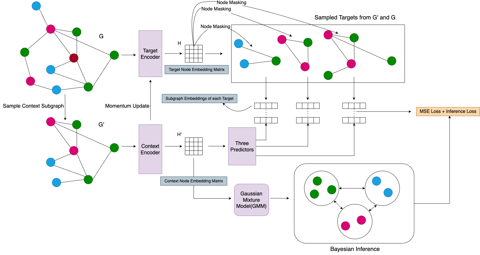
Figure 1: Overall Framework Diagram

3.1 Preliminaries

Consider the definition of a Graph $G=(V,E)$. Let $V$ be the set of vertices $\{v_{1},v_{2},v_{3}....v_{n_{v}}\}$ and $E$ be the set of edges $\{e_{1},e_{2},e_{3}...e_{n_{e}}\}$. $n_{v},n_{e}$ are the number of nodes and edges respectively in $G$. Each node in $V$ is characterized by a $d$ dimensional vector. This is the initial signal that is populated by either bag of words or binary values depending on the problem considered.

3.2 Loss Function

3.2.1 Joint Predictive Optimization

We sample a subgraph $G^{\prime}$ from graph $G$ by dropping a set of nodes according to a Bernoulli distribution parameterized by success probability $p_{1}$. The subgraph $G^{\prime}$ is passed into the context encoder to output node embeddings $H^{\prime}$ of dimensions $d^{\prime}$. Meanwhile, the graph $G$ is passed into the target encoder to generate node embeddings $H$ with the same dimensions as $H^{\prime}$. At the latent space, we sample 3 target subgraphs from the context subgraph $G^{\prime}$, again according to a Bernoulli distribution with probability $p_{2}$ such that $p_{2}<p_{1}$. The node embeddings of each subgraph are obtained by deactivating the node features of masked nodes, which is followed by global mean pooling operation, thus obtaining embeddings $H^{t}_{1}$,$H^{t}_{2}$ and $H^{t}_{3}$. The context node level embeddings $H^{\prime}$ is passed into 3 predictors, corresponding to the three target subgraphs. The obtained predictions are then pooled by the mean pooling operation, thus resulting in target predictions $H^{\prime}_{1},H^{\prime}_{2},H^{\prime}_{3}$, conditioned on latent variable $H^{\prime}$. We then frame the objective function for the joint predictive component as follows,

$$\mathcal{L}^{J}(\Theta^{C},\Theta^{R})=\frac{1}{T}\Sigma_{k=1}^{k=T}||H^{\prime}_{k}-H^{t}_{k}||^{2}$$ (1)

where $T$ is the total number of targets, $\Theta^{C}$ is the weight matrix of the context encoder and $\Theta^{R}$ is the weight matrix of the target encoder. The objective is computed at the latent space with no reconstruction/negative sampling involved.

3.2.2 Node Feature Contribution Optimization

The node embeddings $H^{\prime}$ obtained from passing $G^{\prime}$ into the context encoder are fit in a Gaussian Mixture Model(GMM). We aim to obtain,

$$p(z_{k}=1|h^{\prime}_{n})=\frac{p(h^{\prime}_{n}|z_{k}=1)p(z_{k}=1)}{\Sigma_{j=1}^{j=K}p(h^{\prime}_{n}|z_{j}=1)p(z_{j}=1)}$$ (2)

where $z$ is a latent variable that takes 2 values: one if $h^{\prime}$ comes from Gaussian $k$, and zero otherwise. We can obtain,

$$p(z_{k}=1)=\pi_{k}$$ (3)

$$p(h^{\prime}_{n}|z_{k}=1)=\mathcal{N}(h^{\prime}_{n}|\mu_{k},\Sigma_{k})$$ (4)

where $\pi_{k}$ is the mixing coefficient such that,

$$\Sigma_{k=1}^{k=K}\pi_{k}=1$$ (5)

On replacing these equations in eq.2, we obtain

$$p(z_{k}=1|h^{\prime}_{n})=\frac{\pi_{k}\mathcal{N}(h^{\prime}_{n}|\mu_{k},\Sigma_{k})}{\Sigma\pi_{j}\mathcal{N}(h^{\prime}_{n}|\mu_{j},\Sigma_{j})}=\gamma(z_{nk})$$ (6)

E-Step: In the E-Step, we aim to evaluate,

$$\mathcal{Q}(\theta^{*},\theta)=\mathbb{E}[\ln p(H^{\prime},Z|\theta^{*})]=\Sigma_{Z}p(Z|H^{\prime},\theta)\ln p(H^{\prime},Z|\theta^{*})$$ (7)

from eq.6, we can substitute $\gamma$ in the above equation as,

$$\mathcal{Q}(\theta^{*},\theta)=\Sigma_{Z}\gamma(z_{nk})\ln p(H^{\prime},Z|\theta^{*})$$ (8)

On finding the complete likelihood of the model, we finally have,

$$\mathcal{Q}(\theta^{*},\theta)=\Sigma_{n=1}^{N}\Sigma_{k=1}^{K}\gamma(z_{nk})[\ln\pi_{k}+\ln\mathcal{N}(h^{\prime}_{n}|\mu_{k},\Sigma_{k})]$$ (9)

M-Step: In the M-Step, we aim to find updated parameters $\theta^{*}$ as follows,

$$\theta^{*}=\arg\max_{\theta}\mathcal{Q}(\theta^{*},\theta)$$ (10)

Considering the restriction, $\Sigma_{k=1}^{K}\pi_{k}=1$, eq.9 is modified as follows,

$$\mathcal{Q}(\theta^{*},\theta)=\Sigma_{n=1}^{N}\Sigma_{k=1}^{K}\gamma(z_{nk})[\ln\pi_{k}+\ln\mathcal{N}(h^{\prime}_{n}|\mu_{k},\Sigma_{k})]-\lambda(\Sigma_{k=1}^{k=K}\pi_{k}-1)$$ (11)

The parameters are then determined by finding the maximum likelihood of $\mathcal{Q}$. On taking the derivative with respect to $\pi_{k},\mu_{k},\Sigma_{k}$ and rearranging terms, we finally obtain the update equations for the parameters as follows,

$$\pi_{k}=\frac{\Sigma_{n=1}^{n=N}\gamma(z_{nk})}{N}$$ (12)

$$\mu_{k}^{*}=\frac{\sum_{n=1}^{N}\gamma(z_{nk})h^{\prime}_{n}}{\sum_{n=1}^{N}\gamma(z_{nk})}$$ (13)

$$\sum_{k}^{*}=\frac{\sum_{n=1}^{N}\gamma(z_{nk})(h^{\prime}_{n}-\mu_{k})(h^{\prime}_{n}-\mu_{k})^{T}}{\sum_{n=1}^{N}\gamma(z_{nk})}$$ (14)

Parameter $\Theta^{C}$ Update: Let $V_{g}$ be a vector of pseudo-labels obtained for each node from the Gaussian Mixture Model(GMM) and $V_{k}$ be the vector of pseudo-labels obtained by clustering node embeddings $H^{\prime}$ by K-Means. We update the context encoder parameters $\Theta^{c}$ with the following objective,

$$\mathcal{L}^{G}=\begin{cases}0.5(\frac{V_{g}^{T}H^{\prime}}{\Sigma V_{g}||V_{g}||}-\frac{V_{k}^{T}H^{\prime}}{\Sigma V_{k}||V_{k}||})/\beta,&\text{if}|\frac{V_{g}^{T}H^{\prime}}{\Sigma V_{g}||V_{g}||}-\frac{V_{k}^{T}H^{\prime}}{\Sigma V_{k}||V_{k}||}|<\beta\\ |\frac{V_{g}^{T}H^{\prime}}{\Sigma V_{g}||V_{g}||}-\frac{V_{k}^{T}H^{\prime}}{\Sigma V_{k}||V_{k}||}|-0.5\beta,&\text{otherwise}\par\end{cases}$$ (15)

In the above equation, the context encoder parameters $\Theta^{c}$ are updated by the smooth $L_{1}$ loss function.

3.2.3 Final objective

The context encoder parameters $\Theta^{C}$ are finally updated as follows,

$$\mathcal{L}=\mathcal{L^{J}}+\mathcal{L^{G}}$$ (16)

$$\Theta^{C}\leftarrow\text{optimize}(\Theta^{c},\alpha,\partial_{\Theta^{c}}\mathcal{L})$$ (17)

where, $\alpha$ is the learning rate for the Adam optimizer. The weights of the context and target encoder are randomly initialized by a standard normal distribution. A cosine annealing learning rate scheduler with early stopping is used in all experiments.

3.3 Description of Components and Operations

3.3.1 Context Encoder

The node features from $G^{\prime}$ are passed into the context encoder. The context encoder is a simple 3-layer GCN encoder which predicts 128, 256 and 512 features in each layer respectively. The forward propagation for each layer is described as follows,

$$X^{\prime}=g(\hat{D}^{\frac{-1}{2}}\hat{A}\hat{D}^{\frac{=1}{2}}X\Theta)$$ (18)

$$\hat{A}=A+I$$ (19)

where $\hat{D}$ is the degree matrix, $\hat{A}$ is the adjacency matrix with added self-loops and $\Theta$ is the learned weights matrix. $g$ is a non-linear function. We use ReLU for the first two layers and Tanh for the final layer. The context encoder is an online encoder whose weights are updated by gradient descent.

3.3.2 Target Encoder

The target encoder inputs node features from $G$. Similar to the context encoder, it is a 3-layer GCN encoder with same number of hidden, output dimensions and forward propagation steps. The weights of the target encoder are updated as a moving average of the context encoder as follows,

$$\Theta_{s}^{R}=m\Theta^{R}_{s-1}+(1-m)\Theta_{s}^{C}$$ (20)

where $\Theta^{R}$ is the weights matrix of the target encoder, $\Theta^{C}$ is the weights of the context encoder, $m$ is the momentum parameter and $s$ refers to the $s$th iteration.

3.3.3 Predictor

The predictor consists of 2 GCN layers, both predicting 512 features. The activation function $g$ for both layers is Tanh, in line with the final layer of the target encoder. We use Tanh since it is a bounded function, thus stabilizing the loss computation and optimization.

3.3.4 Global Mean Pooling Operation

The global mean pool operation for a graph $G$ is given as follows,

$$r=\frac{1}{N}\Sigma_{n=1}^{n=N}x_{n}$$ (21)

where $x_{n}$ refers to the node features of node $n$ and $N$ is the total number of nodes in graph $G$

4 Experiments

4.1 Experimental Setting

4.1.1 Datasets

In our experiments, we evaluate our proposed framework on six publicly available benchmark datasets for node representation learning and classification. The datasets are, namely, Cora([17]), Pubmed([18]), Citeseer([17]), Amazon Photos([19]), Amazon Computers([19]) and Coauthor CS([19]). Cora consists of 2708 scientific publications classified into one of seven classes, Citeseer consists of 3312 scientific publications classified into one of six classes and Pubmed consists of 19717 scientific publications pertaining to diabetes classified into one of three classes. In Amazon Photos and Amazon Computers, nodes represent goods and edges represent that two goods are frequently bought together. The product reviews are represented as bag-of-words features. Coauthor CS contains paper keywords for each author’s papers. Nodes represent authors that are connected by an edge if they co-authored a paper.

4.1.2 Evaluation Methodology

The embeddings are evaluated on node classification, whose performance is quantified by accuracy. We follow the same evaluation protocol as used in [20], [12], [11] etc.

4.1.3 Evaluation Protocol

For all downstream tests, we follow the linear evaluation protocol on graphs where the parameters of the backbone/encoder are frozen during inference time. Only the prediction head, which is a single GCN layer, is trained for node classification. For evaluation purposes, we use the default number for train/val/test splits for the citation networks i.e. Cora, Pubmed, Citeseer which are 500 validation and 1000 testing nodes. The train/val/test splits for the remaining datasets, namely, Amazon Photos, Amazon Computers and Coauthor CS are according to [19]. Unless otherwise mentioned, performance is averaged over 10 independent runs with different random seeds and splits for all six evaluation datasets. We report the mean and standard deviation obtained across 10 runs.

4.1.4 Environment

To ensure a fair comparison, for all datasets, we use the same number of layers for the GNN encoder and the same number of features at each hidden layer. The encoder predicts 512 hidden features in the latent space for all datasets. The number of output features of the final classification head is the only parameter varied. We use a Cosine Annealing learning rate scheduler with warm restarts after 75 epochs, and early stopping is employed for all experiments.

4.2 Evaluation Results

4.2.1 Performance on Node Classification

As mentioned earlier, we use the linear evaluation protocol and report the mean and standard deviation of classification accuracy on the test nodes over 10 runs on different folds or splits with different seeds. We compare our proposed approach with supervised and fine-tuned model baselines. For supervised node classification, we compare our proposed approach against Multi Layer Perceptron(MLP),Graph Convolution Network(GCN)([21]), Graph Attention Network(GAT)([20]), Simplified GCN([22]), Logistic Regression and GraphSAGE([23]). For GraphSAGE, we use the mean, maxpool and meanpool variants as described in [19]. We have compared our model’s performance against supervised baselines in table 1. For self-supervised and fine-tuned node classification, we compare our proposed approach against DGI, MVGRL([5]), GRACE([6]), CCA-SSG([9]), SUGRL([24]), S3-CL([12]), GraphMAE([10]), GMI([25]), BGRL([13]) and ParetoGNN([11]). Table 2 contains our model’s performance against self-supervised baselines. The proposed approach demonstrates superior performance across both small and large datasets, showcasing its scalability and robustness. In supervised node classification (Table 1), our method achieves the highest accuracy on Cora ($89.8\pm 0.9$), Citeseer ($77.0\pm 0.9$), and Amazon Photos ($94.5\pm 0.5$), outperforming state-of-the-art models like BGRL and GraphMAE. Specifically, compared to BGRL, our approach shows significant improvements on Cora and Citeseer, while maintaining competitive results on Pubmed and Coauthor CS. Table 3 highlights a direct comparison with BGRL and ParetoGNN, where our method outperforms both on Photos ($94.5\pm 0.5$) and CS ($93.6\pm 0.4$), and remains competitive on Computers. These results underscore the approach’s adaptability and strong performance across diverse dataset sizes, particularly excelling over BGRL and ParetoGNN in key benchmarks. Owing to the ability of our proposed approach to avoid noisy features, representation collapse, and leverage semantic information, our proposed model performs well on small and unstable datasets such as cora and citeseer and large datasets such as Amazon and Coauthor.

Method	Cora	Citeseer	Pubmed	Amazon P	Amazon Comp.	Coauthor CS
MLP	$55.2\pm 0.4$	$46.5\pm 0.5$	$71.4\pm 0.3$	$78.5\pm 0.2$	$44.9\pm 5.8$	$76.5\pm 0.3$
GCN	$81.5\pm 1.3$	$\underline{71.9\pm 1.9}$	$77.8\pm 2.9$	$91.2\pm 1.2$	$\underline{82.6\pm 2.4}$	$91.1\pm 0.5$
GAT	$\underline{81.8\pm 0.3}$	$71.4\pm 1.8$	$78.7\pm 2.3$	$85.7\pm 20.3$	$78.0\pm 19.0$	$90.5\pm 0.6$
Simplified GCN	$81.5\pm 0.2$	$73.1\pm 0.1$	$\underline{79.7\pm 0.4}$	$88.3\pm 1.1$	N/A	$\underline{91.5\pm 0.3}$
GraphSage Mean	$79.2\pm 7.7$	$71.6\pm 1.9$	$77.4\pm 2.2$	$\underline{91.4\pm 1.3}$	$82.4\pm 1.8$	$91.3\pm 2.8$
GraphSage MaxPool	$76.6\pm 1.9$	$67.5\pm 2.3$	$76.1\pm 2.3$	$90.4\pm 1.3$	N/A	$85.0\pm 1.1$
GraphSage MeanPool	$77.9\pm 2.4$	$68.6\pm 2.4$	$76.5\pm 2.4$	$90.7\pm 1.6$	$79.9\pm 2.3$	$89.6\pm 0.9$
Logistic Regression	$57.1\pm 2.3$	$61.0\pm 2.2$	$64.1\pm 3.1$	$73.0\pm 6.5$	$64.1\pm 5.7$	$86.4\pm 0.9$
Ours	$\mathbf{89.8\pm 0.9}$	$\mathbf{77.0\pm 0.9}$	$\mathbf{85.7\pm 1.0}$	$\mathbf{94.5\pm 0.5}$	$\mathbf{88.0\pm 0.6}$	$\mathbf{93.6\pm 0.4}$

Table 1: Supervised Node Classification. The values indicate the accuracy achieved on node classification by several methods. A higher value indicates better performance. The best score is marked in bold and the second best score is underlined. N/A indicates that the score was not reported for a particular dataset by the original authors.

Method	Cora	Citeseer	Pubmed	Amazon P	Amazon Comp.	Coauthor CS
DGI	$81.7\pm 0.6$	$71.5\pm 0.7$	$77.3\pm 0.6$	$83.1\pm 0.3$	$83.6\pm 0.2$	$90.0\pm 0.3$
MVGRL	$82.9\pm 0.7$	$72.6\pm 0.7$	$79.4\pm 0.3$	$87.3\pm 0.1$	$82.8\pm 0.1$	$91.3\pm 0.1$
GRACE	$80.0\pm 0.4$	$71.7\pm 0.6$	$79.5\pm 1.1$	$81.8\pm 0.8$	$89.5\pm 0.3$	$71.1\pm 0.2$
CCA-SSG	$84.2\pm 0.4$	$73.1\pm 0.3$	$81.6\pm 0.4$	$93.1\pm 0.1$	$88.7\pm 0.3$	$\underline{93.3\pm 0.2}$
SUGRL	$83.4\pm 0.5$	$73.0\pm 0.4$	$81.9\pm 0.3$	$\underline{93.2\pm 0.4}$	$\underline{88.9\pm 0.2}$	$92.2\pm 0.5$
S3-CL	$\underline{84.5\pm 0.4}$	$\underline{74.6\pm 0.4}$	$80.8\pm 0.3$	$89.0\pm 0.5$	N/A	$93.1\pm 0.4$
GraphMAE	$84.2\pm 0.4$	$73.1\pm 0.4$	$83.9\pm 0.3$	$90.7\pm 0.4$	$79.4\pm 0.5$	$93.1\pm 0.1$
GMI	$82.7\pm 0.2$	$73.3\pm 0.3$	$77.3\pm 0.6$	$83.1\pm 0.3$	N/A	$91.0\pm 0.0$
BGRL	$83.8\pm 1.6$	$72.3\pm 0,9$	$\mathbf{86.0\pm 0.3}$	$93.2\pm 0.3$	$\mathbf{90.3\pm 0.2}$	$93.3\pm 0.1$
Ours	$\mathbf{89.8\pm 0.9}$	$\mathbf{77.0\pm 0.9}$	$\underline{85.7\pm 1.0}$	$\mathbf{94.5\pm 0.5}$	$88.0\pm 0.6$	$\mathbf{93.6\pm 0.4}$

Table 2: Self Supervised followed by Fine-Tuning. The values indicate the accuracy achieved on node classification by several SSL methods. A higher value indicates better performance. The best score is marked in bold and the second best score is underlined. N/A indicates that the score was not reported for a particular dataset by the original authors.

Method	Photos	Computers	CS
BGRL	$93.2\pm 0.3$	$90.3\pm 0.2$	$93.3\pm 0.1$
ParetoGNN	$93.8\pm 0.3$	$\mathbf{90.7\pm 0.2}$	$92.2\pm 0.1$
Ours	$\mathbf{94.5\pm 0.5}$	$88.0\pm 0.6$	$\mathbf{93.6\pm 0.4}$

Table 3: Comparision with BGRL and ParetoGNN on datasets introduced in [19]. The best score for each dataset is marked in bold.

4.2.2 Study on GMM Cluster Optimization

In this section, we evaluate the significance of the constraint in our loss function. Our approach combines learning sub-graph embeddings with optimizing node embeddings using pseudo-labels derived from a Gaussian Mixture Model (GMM). These pseudo-labels, converted to normalized scores, serve as a constraint in the original loss function for subgraph embeddings. Table 4 illustrates the performance of our method with and without this constraint, demonstrating a substantial improvement when the GMM-derived pseudo-label scores are incorporated. This finding is particularly noteworthy as it indicates that computationally expensive processes like negative sampling, commonly used in graph contrastive learning, may not be essential for optimizing node embeddings. Our approach thus offers a more efficient alternative while maintaining, and even enhancing, performance in graph representation learning tasks.

Method	Cora	Citeseer	Pubmed	Amazon P	Amazon Comp.	Coauthor CS
Without Bayesian Inference	89.0	74.1	84.2	93.4	85.0	93.2
With Bayesian Inference	$\mathbf{89.8}$	$\mathbf{77.0}$	$\mathbf{85.7}$	$\mathbf{94.5}$	$\mathbf{88.0}$	$\mathbf{94.5}$

Table 4: Ablation Study for Loss Function.The best score for each dataset is marked in bold.

4.2.3 Study on Momentum Parameter $m$

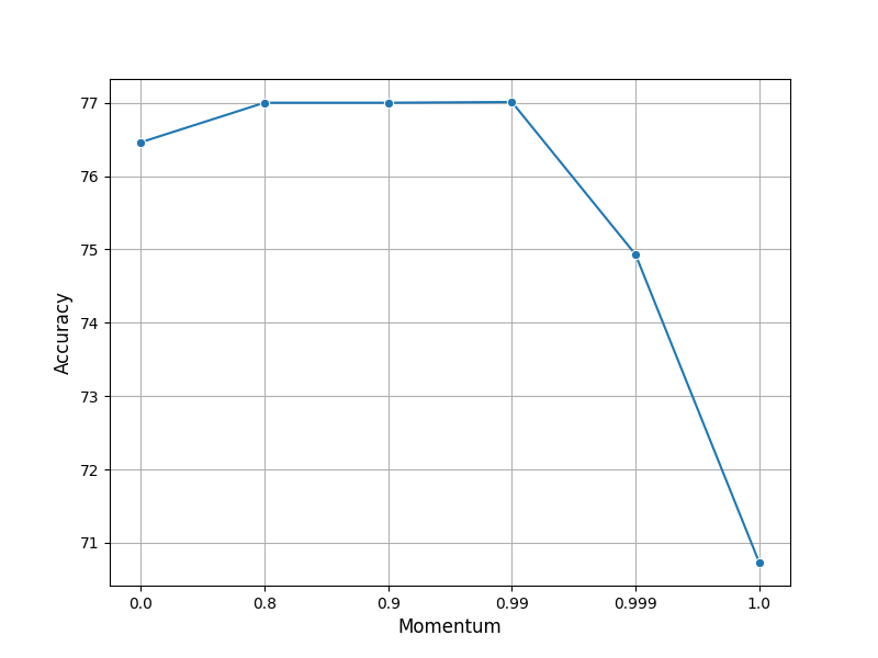
Figure 2: Variation of accuracy with respect to momentum parameter $m$ on Citeseer

Figure 2 represents the change in performance with respect to the momentum parameter on the citeseer dataset. The ideal values for $m$ may range between 0.8 and 0.9. As $m\rightarrow 1$, the weights of the target encoder update by very small steps, thereby slowing down learning. This is further indicated by the drop in performance. For all our experiments, we use $m=0.9$

4.2.4 Spread of Embeddings

Figure 3 represents the spread of node embeddings across all 6 tested datasets. As mentioned earlier, the node embeddings are bounded between -1 and 1 since the final layer activation function is Tanh. The plots indicate that the node embeddings are evenly distributed with a high dispersion indicating a higher variance, implying that the embeddings span a wide range of values. This is a key indicator that our proposed method effectively prevents node representations from clustering too closely, ensuring that each node maintains a distinct position within the embedding space. This controlled spread minimizes overlap between node embeddings, thereby enhancing the uniqueness and robustness of the overall representation.

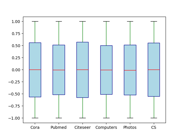
Figure 3: Box plot representing the learned embeddings on all tested datasets

4.2.5 Study on Performance against Test Time Node Feature Distortion

We evaluate the performance of our method on node classification by augmenting the test splits. We sample $p$ percentage test nodes randomly and replace their node features with points sampled from a standard Gaussian distribution. We evaluate the performance of the distorted test nodes on Amazon Computers, Amazon Photos and Coauthor CS by varying $p$ between 10% to 40% and report their performance differences in table 5. In this study, we only use Co-author and Amazon networks since citation networks tend to be unstable on evaluation as indicated in [19]. Despite no further fine-tuning on distorted node features, the average performance drop on Amazon Photos and Computers is only 2.96% and 4.01% respectively. This indicates the ability of the joint framework to generalize on noise-augmented views as well. According to our hypothesis, we believe this is due to the nature of joint predictive embedding learning where a higher variation in context and target embeddings is required for better generalization.

Ratio of Nodes Distorted	Photos	Computers	Coauthor CS
0.10	-3.3%	-3.8%	-3.3%
0.15	-0.8%	-3.4%	-1.2%
0.20	-3.7%	-3.3%	-3.3%
0.25	-2.9%	-4.6%	-7.7%
0.30	-3.9%	-4.3%	-5.9%
0.35	-2.4%	-4.0%	-6.6%
0.40	-3.7%	-4.7%	-9.6%

Table 5: Performance on distorting node features at test time. Values represent the percentage decrease in the model’s performance compared to its original score. A lower value indicates better performance.

5 Conclusion

In this paper, we propose a novel Graph Self-Supervised Learning (Graph-SSL) framework that combines joint predictive embedding and pseudo-labeling to effectively capture global knowledge while avoiding noisy features and bypassing contrastive methods such as negative sampling and reconstruction. The joint predictive embedding framework leverages the context-target relationship between node embeddings in the latent space by predicting multiple target embeddings for a single context. This approach, combined with the optimization of node feature contributions to pseudo-labels, enables a lightweight Graph Neural Network (GNN) encoder to capture intricate patterns in both graph structure and node features without requiring the stacking of multiple layers or encoders. Additionally, our method addresses the node representation collapse problem by incorporating information from multiple targets for a single context, ensuring robust and diverse embeddings. Through extensive experiments on multiple benchmark graph datasets, we demonstrate that our proposed framework achieves superior performance compared to several state-of-the-art graph self-supervised learning methods.

References

- [1] Seiji Maekawa, Koki Noda, Yuya Sasaki, et al. Beyond real-world benchmark datasets: An empirical study of node classification with gnns. Advances in Neural Information Processing Systems, 35:5562–5574, 2022.
- [2] Muhan Zhang and Yixin Chen. Link prediction based on graph neural networks. Advances in neural information processing systems, 31, 2018.
- [3] Yuecheng Li, Jialong Chen, Chuan Chen, Lei Yang, and Zibin Zheng. Contrastive deep nonnegative matrix factorization for community detection. In ICASSP 2024-2024 IEEE International Conference on Acoustics, Speech and Signal Processing (ICASSP), pages 6725–6729. IEEE, 2024.
- [4] Petar Veličković, William Fedus, William L Hamilton, Pietro Liò, Yoshua Bengio, and R Devon Hjelm. Deep graph infomax. arXiv preprint arXiv:1809.10341, 2018.
- [5] Kaveh Hassani and Amir Hosein Khasahmadi. Contrastive multi-view representation learning on graphs. In International conference on machine learning, pages 4116–4126. PMLR, 2020.
- [6] Yanqiao Zhu, Yichen Xu, Feng Yu, Qiang Liu, Shu Wu, and Liang Wang. Deep graph contrastive representation learning. arXiv preprint arXiv:2006.04131, 2020.
- [7] Yuhu Wang, Jinyong Wen, Chunxia Zhang, and Shiming Xiang. Graph aggregating-repelling network: Do not trust all neighbors in heterophilic graphs. Neural Networks, 178:106484, 2024.
- [8] Wei Jin, Xiaorui Liu, Xiangyu Zhao, Yao Ma, Neil Shah, and Jiliang Tang. Automated self-supervised learning for graphs. arXiv preprint arXiv:2106.05470, 2021.
- [9] Hengrui Zhang, Qitian Wu, Junchi Yan, David Wipf, and Philip S Yu. From canonical correlation analysis to self-supervised graph neural networks. Advances in Neural Information Processing Systems, 34:76–89, 2021.
- [10] Zhenyu Hou, Xiao Liu, Yukuo Cen, Yuxiao Dong, Hongxia Yang, Chunjie Wang, and Jie Tang. Graphmae: Self-supervised masked graph autoencoders. In Proceedings of the 28th ACM SIGKDD Conference on Knowledge Discovery and Data Mining, pages 594–604, 2022.
- [11] Mingxuan Ju, Tong Zhao, Qianlong Wen, Wenhao Yu, Neil Shah, Yanfang Ye, and Chuxu Zhang. Multi-task self-supervised graph neural networks enable stronger task generalization. arXiv preprint arXiv:2210.02016, 2022.
- [12] Kaize Ding, Yancheng Wang, Yingzhen Yang, and Huan Liu. Eliciting structural and semantic global knowledge in unsupervised graph contrastive learning. In Proceedings of the AAAI Conference on Artificial Intelligence, volume 37, pages 7378–7386, 2023.
- [13] Shantanu Thakoor, Corentin Tallec, Mohammad Gheshlaghi Azar, Mehdi Azabou, Eva L Dyer, Remi Munos, Petar Veličković, and Michal Valko. Large-scale representation learning on graphs via bootstrapping. arXiv preprint arXiv:2102.06514, 2021.
- [14] Ming Jin, Yizhen Zheng, Yuan-Fang Li, Chen Gong, Chuan Zhou, and Shirui Pan. Multi-scale contrastive siamese networks for self-supervised graph representation learning. arXiv preprint arXiv:2105.05682, 2021.
- [15] Mahmoud Assran, Quentin Duval, Ishan Misra, Piotr Bojanowski, Pascal Vincent, Michael Rabbat, Yann LeCun, and Nicolas Ballas. Self-supervised learning from images with a joint-embedding predictive architecture. In Proceedings of the IEEE/CVF Conference on Computer Vision and Pattern Recognition, pages 15619–15629, 2023.
- [16] Zhengcong Fei, Mingyuan Fan, and Junshi Huang. A-jepa: Joint-embedding predictive architecture can listen. arXiv preprint arXiv:2311.15830, 2023.
- [17] Prithviraj Sen, Galileo Namata, Mustafa Bilgic, Lise Getoor, Brian Galligher, and Tina Eliassi-Rad. Collective classification in network data. AI magazine, 29(3):93–93, 2008.
- [18] Galileo Namata, Ben London, Lise Getoor, Bert Huang, and U Edu. Query-driven active surveying for collective classification. In 10th international workshop on mining and learning with graphs, volume 8, page 1, 2012.
- [19] Oleksandr Shchur, Maximilian Mumme, Aleksandar Bojchevski, and Stephan Günnemann. Pitfalls of graph neural network evaluation. arXiv preprint arXiv:1811.05868, 2018.
- [20] Petar Veličković, Guillem Cucurull, Arantxa Casanova, Adriana Romero, Pietro Lio, and Yoshua Bengio. Graph attention networks. arXiv preprint arXiv:1710.10903, 2017.
- [21] Thomas N Kipf and Max Welling. Semi-supervised classification with graph convolutional networks. arXiv preprint arXiv:1609.02907, 2016.
- [22] Felix Wu, Amauri Souza, Tianyi Zhang, Christopher Fifty, Tao Yu, and Kilian Weinberger. Simplifying graph convolutional networks. In International conference on machine learning, pages 6861–6871. PMLR, 2019.
- [23] Will Hamilton, Zhitao Ying, and Jure Leskovec. Inductive representation learning on large graphs. Advances in neural information processing systems, 30, 2017.
- [24] Yujie Mo, Liang Peng, Jie Xu, Xiaoshuang Shi, and Xiaofeng Zhu. Simple unsupervised graph representation learning. In Proceedings of the AAAI conference on artificial intelligence, volume 36, pages 7797–7805, 2022.
- [25] Zhen Peng, Wenbing Huang, Minnan Luo, Qinghua Zheng, Yu Rong, Tingyang Xu, and Junzhou Huang. Graph representation learning via graphical mutual information maximization. In Proceedings of The Web Conference 2020, pages 259–270, 2020.