Fair Vertex Problems Parameterized by Cluster Vertex Deletion

Abstract

We study fair vertex problem metatheorems on graphs within the scope of structural parameterization in parameterized complexity. Unlike typical graph problems that seek the smallest set of vertices satisfying certain properties, the goal here is to find such a set that does not contain too many vertices in any neighborhood of any vertex. Formally, the task is to find a set $X\subseteq V(G)$ of fair cost $k$, i.e., such that for all $v\in V(G)$ $|X\cap N(v)|\leq k$. Recently, Knop, Masařík, and Toufar [MFCS 2019] showed that all fair $\mathsf{MSO}_{1}$ definable problems can be solved in $\mathsf{FPT}$ time parameterized by the twin cover of a graph. They asked whether such a statement would be achievable for a more general parameterization of cluster vertex deletion, i.e., the smallest number of vertices required to be removed from the graph such that what remains is a collection of cliques.

In this paper, we prove that in full generality this is not possible by demonstrating a $\mathsf{W[1]}$-hardness. On the other hand, we give a sufficient property under which a fair $\mathsf{MSO}_{1}$ definable problem admits an $\mathsf{FPT}$ algorithm parameterized by the cluster vertex deletion number. Our algorithmic formulation is very general as it captures the fair variant of many natural vertex problems such as the Fair Feedback Vertex Set, the Fair Vertex Cover, the Fair Dominating Set, the Fair Odd Cycle Transversal, as well as a connected variant of thereof. Moreover, we solve the Fair $[\sigma,\rho]$-Domination problem for $\sigma$ finite, or $\sigma=\mathbb{N}$ and $\rho$ cofinite. Specifically, given finite or cofinite $\rho\subseteq\mathbb{N}$ and finite $\sigma$, or $\rho\subseteq\mathbb{N}$ cofinite and $\sigma=\mathbb{N}$, the task is to find set of vertices $X\subseteq V(G)$ of fair cost at most $k$ such that for all $v\in X$, $|N(v)\cap X|\in\sigma$ and for all $v\in V(G)\setminus X$, $|N(v)\cap X|\in\rho$.

1 Introduction

We investigate the parameterized complexity of a large class of vertex graph problems under a structural parameterization. In particular, we study fair problems that are becoming more popular in recent years while their history can be traced back to the 80’s [LinSahni]. The paradigm of the fair problems is that we seek a solution, usually represented as a subset of some universe, which is well-distributed within the given underlying structure but does not necessarily have the smallest possible size. The standard formal formulation of the idea above which is tailored to graph problems uses the fair cost function as a measure of well-distributedness. Given a graph $G$, we define the fair cost ($\mathsf{fc}$) of set $X\subseteq V(G)$ as $\mathsf{fc}(X)\coloneqq\max_{v\in V(G)}|N(v)\cap X|$, where $N(v)$ is an open neighborhood of vertex $v$ in $G$. Then the fair vertex problems on graphs are graph problems defined as set $X\subseteq V(G)$ of the smallest fair cost among all vertex subsets satisfying some property. As we wish to solve a large collection of problems, we need to formally characterize what properties we care about. For that, we use a concept of graph logic which is a standard tool that allows us to specify a collection of problems stateable using common tools. For example, in the $\mathsf{MSO}_{1}$ logic, for which we design our main $\mathsf{FPT}$ algorithm, we can define many standard graph properties such as $k$-colorability, acyclicity, and even the connectivity of a set. See Section˜2.1 for more details. Before stating a formal definition, we wish to bring up one detail which we would like to discuss: We separate the class of problems into two categories. First, where the logic does not have access to set $X\subseteq V(G)$ which is only used to compute the fair cost. Second, on the other hand, provides access to $X$ which plays the role of a free variable in the formula. Therefore, we provide two distinct problem formulations below. We follow the notation established in [KMT19], where L represent an abstract logic.

Fair Vertex $\mathsf{L}$ Deletion
Input:	An undirected graph $G$, $k\in\mathbb{N}$, and a sentence $\varphi$ in logic L.
Question:	Is there a set $X\subseteq V(G)$ of fair vertex cost at most $k$ such that $G[{V(G)\setminus X}]\models\varphi$?

In the above definition, $G[{Y}]$ denotes $G$ induced by $Y\subseteq V(G)$. We can observe that this definition is rather general but it does not capture, for example, the Fair Dominating set problem, i.e., a problem asking for a set $X\subseteq V(G)$ such that for all $v\in V(G)$ $N[v]\cap X\neq\emptyset$. Hence, we present the more powerful variant where we allow free variables.

$\ell$-Fair Vertex $\mathsf{L}$ Evaluation
Input:	An undirected graph $G$, $k\in\mathbb{N}$, and a formula $\varphi(X_{1},\ldots,X_{\ell})$ with $\ell$ free variables in logic L.
Question:	Are there sets $W_{1},\ldots,W_{\ell}$ of vertices each of fair vertex cost at most $k$ such that $G\models\varphi(W_{1},\ldots,W_{\ell})$?

In the special case of $\ell=1$, we say only $\mathsf{L}$-FairVE. So far, we defined the fair vertex problems when provided with logic $\mathsf{L}$ and graph $G$, where the aim is to find a set $X\subseteq V(G)$ of the smallest fair cost that satisfies some formula of $\mathsf{L}$. To speak about particular problems, we often use a template where we say fair -something- problem if the -something- problem can be described in some $\mathsf{L}$ and, therefore, its fair variant belongs to the $\mathsf{L}$-FairVE problems. An important first such example is the Fair Vertex Cover problem, which can be described in $\mathsf{FO}$ logic by a simple formula stating that for all vertices $x,y\not\in X$, we have $xy\not\in E(G)$. Note an important detail that we do not count the access to set $X$ representing the free variable as using a set variable. In fact, we can even express the above in the deletion variant and so, the Fair Vertex Cover belongs to the Fair Vertex $\mathsf{FO}$ Deletion problems.

We can easily modify the fair vertex problem definitions to edge problems where we seek $F\subseteq E(G)$ subject to edge fair cost function defined as $\mathsf{fc}(F)\coloneqq\max_{v\in V(G)}\text{deg}_{F}(v)$, where $\text{deg}_{F}(v)$ measures the number of edges incident to vertex $v$ that are in $F$. The edge variant was the original studied variant in early works [LinSahni, KLS10Kam, Kolman09onfair] until the vertex variant was formally defined in 2017 [MT20]. Edge variant is important for the context, but in the current paper we only explore the fair vertex problems and, therefore, we refrain from formal definitions. For more details on the topic see [KMT19].

In this paper, we study the fair vertex problems under structural parameterization. Very recently, in 2023, Gima and Otachi [GimaOtachi] showed that $\ell$-Fair Vertex $\mathsf{MSO}_{2}$ Evaluation is $\mathsf{FPT}$ parameterized by the vertex integrity and the size of the formula. This is complemented with $\mathsf{W[1]}$-hardness of the Fair Vertex Cover problem even when parameterized by treedepth and feedback vertex set combined [KMT19]. Notice that there is very little gap between those parameters, so the situation on the sparse side of the spectrum seems to be relatively understood. On the other hand, we know much less about dense graph parameters. Knop, Koutecký, Masařík, and Toufar [KKMT] showed that $\ell$-Fair Vertex $\mathsf{MSO}_{1}$ Evaluation is $\mathsf{FPT}$ parameterized by the neighborhood diversity and the size of the formula. Note that $\mathsf{MSO}_{1}$ cannot be extended to $\mathsf{MSO}_{2}$ on dense graph parameters because $\mathsf{MSO}_{2}$ model-checking on cliques is not even in $\mathsf{XP}$ unless $\mathsf{E}=\mathsf{NE}$ [CMR, Lampis14]. Parameterization by the twin cover is explored in [KMT19] and the $\mathsf{MSO}_{1}$-FairVE is $\mathsf{FPT}$ parameterized by the twin cover and the size of the formula while $\ell$-Fair Vertex $\mathsf{MSO}_{1}$ Evaluation is already $\mathsf{W[1]}$-hard under the same parameterization. The question raised in [KMT19] was whether the $\mathsf{MSO}_{1}$-FairVE remains $\mathsf{FPT}$ even when parameterized by the stronger parameter of the cluster vertex deletion. The cluster vertex deletion number is the size of the smallest set $D\subseteq V(G)$ such that $G-D$ (i.e., $G[V(G)\setminus D]$) is a collection of disjoint cliques. We denote a set $D\subseteq V(G)$ such that $G-D$ is a collection of disjoint cliques a modulator of graph $G$. The cluster vertex deletion number is a well-known optimization problem; see e.g., [IKP23] for a very recent overview of results. Nevertheless, it has already been successfully used as a structural graph parameter to provide $\mathsf{FPT}$ algorithms for various graph problems in past two years [BKR23, GKKMV23, KS23]. In this paper, we resolve the general question negatively, while providing a very extensive collection of problems that do admit still an $\mathsf{FPT}$ algorithm under our parameterization. We refer to Figure˜1 for a visual overview of the results and graph class relations.

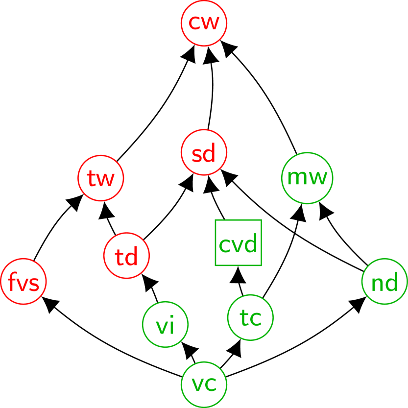
(a) Parameterized complexity of the Fair Vertex Cover problem.

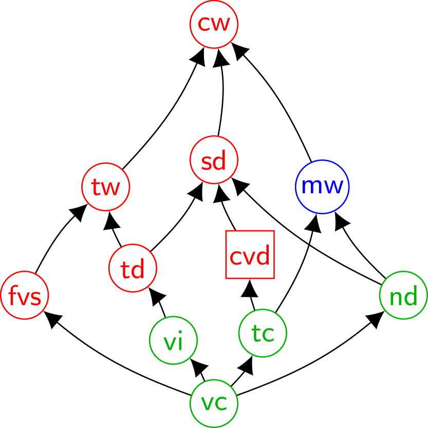
(b) Parameterized complexity of the $\mathsf{MSO}_{1}$-FairVE problem.

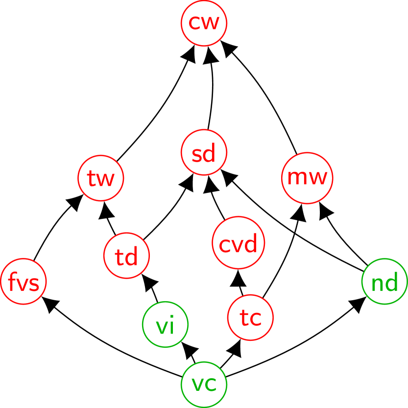
(c) Parameterized complexity of the $\ell$-Fair Vertex $\mathsf{MSO}_{1}$ Evaluation problem.

Figure 1: Parameterized complexity the fair vertex problems. The green color means there is an $\mathsf{FPT}$ algorithm parameterized by the structural parameter (and the size of the formula if it applies). The red color highlights parameters for which there is $\mathsf{W[1]}$-hardness result and the blue color marks yet unknown. Results bounded in rectangle are new in this paper.

Related Results.

The concept of Fair Problems has been extended to include local cardinality constraints, as introduced by Szeider [Szeider:11]. For a graph $G$ with cardinality constraints $\alpha(v)\subseteq[n]$ for all $v\in V(G)$. The solution is a subset $W\subseteq V(G)$ such that $|W\cap N(v)|\in\alpha(v)$ for all $v\in V(G)$. A notable special case, introduced in [KKMT], is called linear local cardinality constraints, where all $\alpha(v)$ forms an interval. Local linear problems were further studied in [Knop2021]. Observe that the fair vertex problems with fair cost $f$ represent the simplest local cardinality constraints, where $\alpha(v)=[f]$ for all $v\in V(G)$.

There was also some interest in exploring particular fair problems parameterized by their solution size, see e.g., [JRS, KMMS21]. Papers [IKKPS25, JRS, FairHighwayDimension] studied an extension of the fair concept into set, specifically introducing and tackling the fair hitting set problem. Moreover, [FairHighwayDimension] shows that the Fair Vertex Cover problem is $\mathsf{NP}$-complete for any $k\geq 4$ even on planar graphs, where $k$ is the fair cost of the solution.

1.1 Our Results

Here, we closely describe our results. First, we state our hardness theorem which is answering a general case of a question posted in [KMT19]. Notice that the hardness is for the most restricted (deletion) version of metatheorems where only a sentence in $\mathsf{FO}$ logic is used after the deletion of a set.

Theorem 1.1 (Hardness).

The Fair Vertex $\mathsf{FO}$ Deletion problem is $\mathsf{W[1]}$-hard parameterized by the cluster vertex deletion number and the size of the formula.

To state the positive result precisely and formally we need to introduce much more model-checking background and tools which we do in Section˜3. It would be too technical to state it at this point in the introduction. We would rather give an overview, intuition, and a less formal statement here. We also explain the methods of our proof and we conclude with the list of fair problems which we show to be solvable in $\mathsf{FPT}$ time parameterized by the cluster vertex deletion.

A big-picture strategy of our proof can be summarized as follows. First, we characterize all the objects, called shapes, that can be viewed as classes of equivalence from the perspective of the formula. That means we can check the truthfulness of the formula on the shape. At the same time, each graph $G$ and a solution $X\subseteq V(G)$ can be reduced to some shape. See Section˜3.2 for the formal definition. A desired outcome of this part of the proof is that the number of shapes is bounded in parameters; the formula size and the size of a modulator. Therefore, all the shapes can be enumerated in $\mathsf{FPT}$ time. A drawback of this strategy is that the fair cost of the input graph $G$ cannot be easily mapped to the shapes and has to be computed. That is what we are going to do. Given a shape we are able to formulate an integer linear program (ILP) to recover the solution of minimal fair cost, which belongs to the equivalence class of this shape. Moreover, such an ILP has the number of variables bounded by our parameters, therefore we utilize the following algorithm originally proposed by Lenstra [Lenstra83].

Theorem 1.2 ([Lenstra83] with an improved running time by Reis and Rothvoss [RR23]).

There is an algorithm that, given an ILP (Integer Linear Program) with $p$ variables and $m$ constraints, finds an optimal solution in time ${\log p}^{\mathcal{O}(p)}\cdot(m\log L)^{\mathcal{O}(1)}$, where $L$ is the maximum absolute value of the coefficients.

Hence, the approach above leads to a solution in $\mathsf{FPT}$ time. Such a general approach was used in both [KMT19, MT20].

However, we faced a few differences which complicated the approach sketched above. After all, under current parameterization, the general problem is $\mathsf{W[1]}$-hard. The first difference is that the objects are more complicated compared with the previous parameterizations [KMT19, MT20], and so the whole model-checking machinery has to be verified to still hold in this case. Certainly, compared to the twin cover, each clique can have many different neighborhoods in the modulator. To prove this part, we used tools developed by Lampis [Lampis12] and by Knop, Masařík, and Toufar [KMT19]. After a meticulous verification we, indeed, know that there are only parametrically many shapes that are relevant with respect to the formula. It is interesting to note that once we have the above, it actually provides an alternative proof of the model-checking (without measuring the fair cost; see Corollary˜3.21) in $\mathsf{FPT}$, time reproving older results, (e.g., implied by [CMR]).

For the second difference, we need to take a closer look at what the shape looks like. It describes the solution on the modulator $D$ exactly, so from now on we focus only on cliques in $G-D$. We partition all the cliques into groups, where each group contains cliques that are either small and have the same number of vertices of identical neighborhoods in the modulator or are large an have all large number of such vertices of identical neighborhoods in the modulator.

For such cliques, shape tells us either how many vertices need to be used in the free variable or how many vertices need to be left out from the free variable. We have such information for all groups of cliques. Although, for groups containing large cliques (which can possibly consist of different sizes of cliques), we only know the shape of a group as a whole and not about the individual cliques in the group. Therefore, we do not know how to assign the cliques of the original graph $G$ to the information described in shape so that we minimize the fair cost. The crucial point in our proof is that as long as the shape states that for all cliques in one group that either all of them are described by how many vertices need to be used in the free variable or all of them are described by how many vertices need to be left out from the free variable, we are able to formulate an integer linear program in bounded dimension that computes the minimum fair cost (Theorem˜1.2). We call shapes that satisfy the above property coherent; see Definition˜3.4 for a formal definition. Let us summarize this statement as an informal main theorem. The formal equivalent is presented in Section˜3.3 as Theorem˜3.10.

Theorem 1.3 (Main informal algorithmic $\mathsf{FPT}$ statement; see Theorem˜3.10 for a formal version).

Let $\varphi(\aleph)$ be a fixed $\mathsf{MSO}_{1}$ formula with one free variable and $G$ be a graph. If there exists a solution of the minimal fair cost whose shape is coherent then we can solve the respective $\mathsf{MSO}_{1}$-FairVE problem in $\mathsf{FPT}$ time parameterized by $|\varphi|$ and $|D_{G}|$.

Surprisingly, observe that the assumptions of the theorem are properties of the problem, and more importantly, we can decide about individual problems whether they satisfy this assumption. We do such a verification in Section˜5. Let us demonstrate an example of such a reasoning for the Fair Vertex Cover problem. Notice that from each clique we need to take either all or all but one vertices to the vertex cover set. Therefore, each such solution leads to a coherent shape, as even the solution on all cliques is described by how many vertices need to be left out from the free variable. It is for each clique either zero or one as reasoned above.

We define several fundamental graph vertex problems that are covered by Theorem˜1.3. We provide only very concise formulation here, for more details see Section˜5. Given a graph and integer $d$ at the input. We describe the problems by expressing how $G-X$ is constrained. Note that in addition to that we are looking for $X$ with fair cost at most $d$. The Fair Feedback Vertex Set problem requires $G-X$ to be a forest. The Fair Odd Cycle Transversal problem requires $G-X$ to be a bipartite graph. Of course, we can impose additional $\mathsf{MSO}_{1}$ expressible constraints on $X$ in all the problems above. In particular, the connectivity constraint on $X$ leads to variants of the problems above that has been well studied in non-fair setting; see e.g., a recent study of those problems parameterize by clique-width [FK23]. We also define the Fair $[\sigma,\rho]$-Domination problem for $\sigma$ finite, or $\sigma=\mathbb{N}$ and $\rho$ cofinite. Such class of problems has been coined by Telle in [T94]. There, the task is to find set of vertices $X\subseteq V(G)$ such that for all $v\in X$, $|N(v)\cap X|\in\sigma$ and for all $v\in V(G)\setminus X$, $|N(v)\cap X|\in\rho$. An important and classical member of the family of problems above is the Fair Dominating Set problem, where $\sigma=\mathbb{N},\rho=\mathbb{N}\setminus\{0\}$.

We conclude with a list of problems that are implied by Theorem˜1.3.

Corollary 1.4.

We can solve the following problems in $\mathsf{FPT}$ time parameterized by the cluster vertex deletion.

• Fair Vertex Cover,

• Fair Feedback Vertex Set,

• Fair Odd Cycle Transversal,

• Fair Dominating Set,

• A connected variant of the preceding problems,

• Fair $[\sigma,\rho]$-Domination problem for $\sigma$ finite, or $\sigma=\mathbb{N}$ and $\rho$ cofinite.

Organization of the paper.

After a short preliminaries (Section˜2) we describe the model-checking toolbox and give proofs related to structural understanding of the problem in Section˜3. Notably, we state the main theorem formally in Section˜3.3. In Section˜4 we provide the algorithmic side of the proof including an ILP formulation of the problem. Then we include Section˜5 which provides problem statements of natural problems that are solved by our main theorem together with proofs that they are covered by it. LABEL:sec:hardness contains the proof of our hardness result. We conclude with short conclusions (LABEL:sec:conc).

2 Preliminaries

We denote $[n]\coloneqq\{0,1,2,\ldots n\}$ and $\mathbb{N}_{\text{odd}}\coloneqq\{2n+1:n\in\mathbb{N}\}$. For a graph $G$ and a set $X\subseteq V(G)$, we denote its complement by $\overline{X}\coloneqq V(G)\setminus X$. A modulator $D\subseteq V(G)$ of $G$ is a set such that $G[{V(G)\setminus D}]$ is a collection of vertex disjoint cliques. For every graph $G$, we denote by $D_{G}$ any fixed modulator of the smallest size. We also assume that a set $D_{G}$ has fixed ordering. For a graph $G$ and its modulator $D_{G}$, we let $\mathcal{C}_{G}$ denote the collection of cliques in $G[{V(G)\setminus D_{G}}]$. For a set $X\subseteq V(G)$ and a vertex $v\in V(G)$, we have $N_{X}(v)\coloneqq N(v)\cap X$, i.e., the neighbors of $v$ in $X$. As we will be analyzing the neighborhoods of vertices in modulator $D_{G}$ of $G$, that is $N_{D_{G}}(v)$, we will use a slightly different notation. We denote all binary vectors of length $d$ by $\mathsf{NT}_{d}$. Recall that we also assumed that vertices in $D_{G}$ are ordered, so that there is a natural bijection between all subsets of $D_{G}$ and vectors in $\mathsf{NT}_{|D_{G}|}$. For each $C\in\mathcal{C}_{G}$ and for each $\mathsf{nT}\in\mathsf{NT}_{|D_{G}|}$, we define $C_{\mathsf{nT}}\coloneqq\{v\in V(C):N_{D_{G}}(v)=\mathsf{nT}\}$ as the set of vertices in $C$ whose neighborhood type is $\mathsf{nT}$. Since we will mostly be using $\mathsf{NT}_{|D_{G}|}$, we will use just $\mathsf{NT}$ when it is clear from the context.

A signature of a clique $C\in\mathcal{C}_{G}$ is a vector $\mathsf{sgn}_{C}$ indexed with neighborhood types. For each $\mathsf{nT}\in\mathsf{NT}$, we set $\mathsf{sgn}_{C}[\mathsf{nT}]\coloneqq|C_{\mathsf{nT}}|$. For $C\in\mathcal{C}_{G}$, we also define $\alpha$-truncated signature ${\mathsf{sgn}^{\alpha}_{C}[\mathsf{nT}]\coloneqq\min(|C_{\mathsf{nT}}|,\alpha)}$. For $\alpha\in\mathbb{N}_{\text{odd}}$, we define an $\alpha$-clique type that is a vector $\mathsf{cT}$ indexed with neighborhood types $\mathsf{nT}\in\mathsf{NT}$ and values from $[\alpha]$ such that for $C\in\mathcal{C}_{G}$, $\mathsf{cT}[\mathsf{nT}]\coloneqq\min(\alpha,|C_{\mathsf{nT}}|)$. We denote $\mathsf{CT}^{(\alpha,|D_{G}|)}\coloneqq[\alpha]^{\mathsf{NT}_{|D_{G}|}}$ set of all $\alpha$-clique types. Clearly, $|\mathsf{CT}^{(\alpha,|D_{G}|)}|=\alpha^{|\mathsf{NT}_{|D_{G}|}|}=\alpha^{2^{|D_{G}|}}$.

2.1 Logic

The formulas of $\mathsf{MSO}_{1}$ logic are those which can be constructed using vertex variables, denoted usually by $x_{i},y_{i},\dots$, set variables denoted usually by $X_{i},Y_{i},\dots$, label classes denoted by $L_{i}$, the predicates $E(x_{i},x_{j}),x_{i}\in L_{j},x_{i}=x_{j}$ operating on vertex variables, standard propositional connectives and the quantifiers $\exists,\forall$ operating on vertex and set variables. The semantics are defined in the usual way, with the $E(x_{i},x_{j})$ predicate being true if and only if $(x_{i},x_{j})\in E$ and labels being interpreted as sets of vertices.

We will also consider two more standard logics in graph theory. An $\mathsf{FO}$ logic only allows quantifications over elements (vertices or edges). A more powerful, $\mathsf{MSO}_{2}$, where in addition to $\mathsf{MSO}_{1}$, even quantification over the set of edges is allowed. It is well known that $\mathsf{FO}$ $\subsetneq$ $\mathsf{MSO}_{1}$ $\subsetneq$ $\mathsf{MSO}_{2}$, where the connectivity, and the Hamiltonian cycle are properties demonstrating strict inclusions, respectively. For more details consult e.g., [CE-book].

Let $\varphi(\aleph)$ be a formula with one free variable. The size of the formula (denoted as $|\varphi|$) is measured in the number of vertex and set quantifiers.

3 Shapes and Model-Checking

In this section, we introduce the terminology needed to prove the correctness of our $\mathsf{FPT}$ algorithm (Theorem˜1.3). Firstly, we define compliant solutions (Section˜3.1), which provide canonical representations of solutions without any loss in either the fair cost or the formula. After that, we give a formal definition of a shape which is the main object used for the model-checking (Section˜3.2). With these foundations, we formally state our main theorem (Theorem˜3.10) in Section˜3.3. Then we introduce additional model-checking tools in Section˜3.4. Section˜3.5 proves two main statements of this section. First, that restricting attention to compliant solutions is sufficient from both model-checking as well as the fair cost perspectives (Lemma˜3.2). Second, provides an equivalence of model-checking of a graph $G$ with compliant $X\subseteq V(G)$ on one side and the respective shape on the other side (Lemma˜3.11). As mentioned, the conclusion of this section is that $\mathsf{MSO}_{1}$ model-checking can be done in $\mathsf{FPT}$ time parameterized by the cluster vertex deletion and the size of the formula (Corollary˜3.21).

3.1 Compliant Set

In this short subsection, we define how well-structured sets of vertices look like. Those sets will play the role of canonical solutions with respect to both the formula and the fair cost. This property is captured by Lemma˜3.2.

Definition 3.1 ($\alpha$-compliant sets).

Let $\alpha$ be a positive integer and $G$ be a graph. Recall that $\mathcal{C}_{G}$ is the collection of cliques in $G-D_{G}$.

We say that $X\subseteq V(G)$ is $\alpha$-compliant if for each $C\in\mathcal{C}_{G}$ and for each $\mathsf{nT}\in\mathsf{NT}$

$$\text{either }|X\cap V(C_{\mathsf{nT}})|\leq\frac{\alpha}{2}\text{ or }|\overline{X}\cap V(C_{\mathsf{nT}})|\leq\frac{\alpha}{2}.$$

Lemma 3.2 (Compliant solution of capped fair cost).

There is a computable function ${f:\mathbb{N}^{2}\rightarrow\mathbb{N}}$ such that for any $\mathsf{MSO}_{1}$ formula $\varphi(\aleph)$ with one free variable, for any graph $G$, and for any $\alpha\in\mathbb{N}_{\text{odd}},\alpha>f(|D_{G}|,|\varphi|)$, the following is true. For each $X\subseteq V(G)$ such that $G\models\varphi(X)$, there exist $X^{\prime}\subseteq V(G)$ such that:

• $X^{\prime}$ is $\alpha$-compliant,

• $G\models\varphi(X^{\prime})$, and

• $\mathsf{fc}(X^{\prime})\leq\mathsf{fc}(X)$.

We postpone the proof to Section˜3.5 as we first need to introduce more model-checking tools before we can prove it. However, the statement gives us a good intuition that we will need to care only of solutions $X$ that are $\alpha$-compliant as the other solutions do not have a better fair cost while having the same expressive power.

3.2 Shapes

Throughout this section, we assume that every solution $X$ is $\alpha$-compliant, for some fixed $\alpha$ that depends only on the formula and the size of the modulator. Recall that, in Lemma˜3.2, we prove that it is sufficient to consider only such solutions.

Now we describe how a solution $X$ satisfying formula $\varphi(\aleph)$ on a graph $G$ can be represented. To do so, we introduce the concept of shapes and solution patterns. We define a solution pattern as a vector indexed with neighborhood types $\mathsf{nT}\in\mathsf{NT}_{d}$ and with values from $[\alpha]$. We denote all solution patterns as $\mathsf{SP}^{(\alpha,d)}\coloneqq[\alpha]^{\mathsf{NT}_{d}}$. Intuitively, every $\mathsf{sP}\in\mathsf{SP}^{(\alpha,|D_{G}|)}$ describes how solution $X$ is distributed over vertices with a specific neighborhood type in a particular clique $C\in\mathcal{C}_{G}$. For a graph $G$ and $\mathsf{sP}\in\mathsf{SP}^{(\alpha,|D_{G}|)}$ and for every $\mathsf{nT}\in\mathsf{NT}_{|D_{G}|}$, whenever $\mathsf{sP}[\mathsf{nT}]<\alpha/2$ then there is exactly $\mathsf{sP}[\mathsf{nT}]$ nodes of type $\mathsf{nT}$ from $C$ in solution $X$. On the other hand if $\mathsf{sP}[\mathsf{nT}]>\alpha/2$, then there are all but $\alpha-\mathsf{sP}[\mathsf{nT}]$ nodes of type $\mathsf{nT}$ from $C$ in solution $X$. We will use shorthand notation $\mathsf{SP}$ for $\mathsf{SP}^{(\alpha,|D_{G}|)}$ , when its clear from the context.

Definition 3.3 (Shapes).

Let $\alpha\in\mathbb{N}_{\text{odd}}$ and $\gamma,d\in\mathbb{N}$. We define $\mathsf{Shapes}^{(\alpha,\gamma,d)}$ as a set of all tuples $(\mathsf{nT}^{*},\mathsf{M})$, where:

1. $\mathsf{nT}^{*}\in\mathsf{NT}_{d}$,

2. $\mathsf{M}$ is a $|\mathsf{SP}^{(\alpha,d)}|\times|\mathsf{CT}^{(\alpha+1,d)}|$ matrix whose entries are from $[\gamma]$, and

3. for each $\mathsf{nT}\in\mathsf{NT}$, $\mathsf{cT}\in\mathsf{CT}^{(\alpha+1,d)}$, and $\mathsf{sP}\in\mathsf{SP}^{(\alpha,d)}$ such that $\mathsf{M}[\mathsf{sP},\mathsf{cT}]>0,\mathsf{cT}[\mathsf{nT}]\leq\alpha$, we have $\mathsf{sP}[\mathsf{nT}]\leq\mathsf{cT}[\mathsf{nT}]$.

We refer to an element $\mathsf{shp}\in\mathsf{Shapes}^{(\alpha,\gamma,d)}$ as a shape.

Observe that each entry in $\mathsf{M}$ can be classified as one of 3 types, described below. We say that particular $(\mathsf{nT},\mathsf{cT})$, where $\mathsf{nT}\in\mathsf{NT}$ and $\mathsf{cT}\in\mathsf{CT}^{(\alpha+1,d)}$, is bounded if $\mathsf{cT}[\mathsf{nT}]\leq\alpha$. Otherwise (i.e., $\mathsf{cT}[\mathsf{nT}]=\alpha+1$), $(\mathsf{nT},\mathsf{cT})$ is unbounded. If $(\mathsf{nT},\mathsf{cT})$ is unbounded we further say that for some $\mathsf{sP}\in\mathsf{SP}^{(\alpha,d)}$:

• either $(\mathsf{nT},\mathsf{cT},\mathsf{sP})$ is fat whenever $\alpha/2<\mathsf{sP}[\mathsf{nT}]$,

• or $(\mathsf{nT},\mathsf{cT},\mathsf{sP})$ is thin whenever $\mathsf{sP}[\mathsf{nT}]<\alpha/2$.

If $(\mathsf{nT},\mathsf{cT})$ is bounded then we say $(\mathsf{nT},\mathsf{cT},\mathsf{sP})$ is bounded for any $\mathsf{sP}\in\mathsf{SP}^{(\alpha,d)}$. Note that as $\alpha$ is odd $(\mathsf{nT},\mathsf{cT},\mathsf{sP})$ is either thin, fat, or bounded. Also note that Condition 3) in Definition˜3.3 is necessary, as it ensures that whenever clique $C$ is bounded, a solution pattern $\mathsf{sP}$ does not describe a solution containing more vertices than there is in respective $\mathsf{nT}$ in $C$.

Now, we can provide intuition about shapes. First, we briefly describe the meaning of the parameters $\alpha,\gamma$. Roughly speaking, $\alpha$ corresponds to the maximum number of vertices of the same neighborhood within a single clique that the formula can distinguish. In other words, once there are more than $\alpha$ such vertices, increasing their number further makes no difference to the formula. On the other hand, $\gamma$ corresponds to the maximum number of cliques of the same clique type the formula can distinguish. We will formalize this intuition in Corollary˜3.15 and Corollary˜3.19. Given $G$ and $\varphi(\aleph)$, we define $\mathsf{Shapes}^{(\alpha,\gamma,|D_{G}|)}$ as a set of all possible shapes the solution sets can take as $\alpha$ and $\gamma$ are computed from $\varphi(\aleph)$ and $D_{G}$. Each such shape, denoted as $\mathsf{shp}$, consists of two parts. First, we describe the portion of the solution set $X$ in the modulator $D_{G}$. More precisely, $X\cap D_{G}$ forms the first part of $\mathsf{shp}$, denoted $\mathsf{nT}^{*}$. The second part is a matrix, that describes how the solution $X$ is distributed over the cliques and their respective neighborhood parts. Notice that the number of all possible shapes is bounded in terms of $\alpha,\gamma,|D_{G}|$, so we can enumerate all of them, and maintain an $\mathsf{FPT}$ complexity.

We proceed with the definition of a well-behaved class of shapes that we call coherent shapes. Those will capture a solution of problems that we will be able to solve in $\mathsf{FPT}$ time.

Definition 3.4 (Coherent shape).

Let $\alpha\in\mathbb{N}_{\text{odd}}$ and $\gamma,d\in\mathbb{N}$. We say that $(\mathsf{nT}^{*},\mathsf{M})=\mathsf{shp}\in\mathsf{Shapes}^{(\alpha,\gamma,d)}$ is coherent if for each $\mathsf{nT}\in\mathsf{NT}$ and $\mathsf{cT}\in\mathsf{CT}^{(\alpha+1,d)}$ such that $(\mathsf{nT},\mathsf{cT})$ is unbounded we have that elements of set $\{(\mathsf{nT},\mathsf{cT},\mathsf{sP})\mid{\mathsf{sP}\in\mathsf{SP}^{(\alpha,d)}}\text{ and }\mathsf{M}[\mathsf{sP},\mathsf{cT}]>0\}$ are either all thin or all fat.

We define a relationship between a set of vertices representing a potential solution in the graph and a shape.

Definition 3.5.

For a graph $G$, clique $C\in\mathcal{C}_{G}$ and $\alpha\in\mathbb{N}_{\text{odd}}$, we say that a set $X$ matches a solution pattern $\mathsf{sP}\in\mathsf{SP}^{(\alpha,|D_{G}|)}$ on clique $C$ if for each $\mathsf{nT}\in\mathsf{NT}_{|D_{G}|}$ it holds that
$|X\cap C_{\mathsf{nT}}|=\begin{cases*}\mathsf{sP}[\mathsf{nT}]&if $\mathsf{cT}[\mathsf{nT}]\leq\alpha$\\ \mathsf{sP}[\mathsf{nT}]&if $\mathsf{cT}[\mathsf{nT}]=\alpha+1$ and $\mathsf{sP}[\mathsf{nT}]<\alpha/2$\\ |C_{\mathsf{nT}}|-(\alpha-\mathsf{sP}[\mathsf{nT}])&if $\mathsf{cT}[\mathsf{nT}]=\alpha+1$ and $\mathsf{sP}[\mathsf{nT}]>\alpha/2$\end{cases*}$

Definition 3.6 (Graph and a set associated with a shape).

Given $(\mathsf{nT}^{*},\mathsf{M})=\mathsf{shp}\in\mathsf{Shapes}^{(\alpha,\gamma,d)}$ we construct a graph $G^{\prime}$ and describe $X^{\prime}\subseteq V(G^{\prime})$ associated with $\mathsf{shp}$:

• $G^{\prime}$ has $d$ vertices in modulator and exactly those represented by vector $\mathsf{nT}^{*}$ are in $X^{\prime}$,

• $G^{\prime}$ contains exactly $\sum_{\mathsf{sP}\in\mathsf{SP}^{(\alpha,d)}}\mathsf{M}[\mathsf{sP},\mathsf{cT}]$ cliques of clique type $\mathsf{cT}$ described by $\mathsf{cT}$-th column $($each clique contains exactly $\mathsf{cT}[\mathsf{nT}]$ vertices of neighbourhood type $\mathsf{nT}$ for each $\mathsf{nT}\in\mathsf{NT})$. Moreover, set $X^{\prime}$ matches solution pattern $\mathsf{sP}\in\mathsf{SP}^{(\alpha,d)}$ on exactly $\mathsf{M}[\mathsf{sP},\mathsf{cT}]$ cliques out of those with clique type $\mathsf{cT}$.

We established that a shape can be interpreted as an instance of a solution. In particular, in Definition˜3.6, we described how to associate a graph $G$ and set $X\subseteq V(G)$ with a specific shape. This allows us to evaluate a formula on $G$ where $X$ is substituted for the free variable. We can view this process as evaluating the formula on the shape directly. This is formalized in the following definition.

Definition 3.7 (Evaluation of shape).

Let $\varphi(\aleph)$ be a fixed formula with one free variable. For each $\mathsf{shp}\in\mathsf{Shapes}^{(\alpha,\gamma,d)}$ we define whether $\mathsf{shp}$ is true or false in the given formula $\varphi(\aleph)$ $($denoted as $\models\varphi(\mathsf{shp}))$. Let $G^{\prime},X^{\prime}$ be a graph and a set associated with $\mathsf{shp}$. Then $\models\varphi(\mathsf{shp})$ if and only if $G^{\prime}\models\varphi(X^{\prime})$.

Now, we describe the formal procedure for reducing the size of a clique $C$. As $X$ is $\alpha$-compliant set we need to preserve at most $\alpha$ vertices in any $C_{\mathsf{nT}}$. Consequently, we can express any $\alpha$-compliant solution as a shape, which we will formally establish in Definition˜3.9.

Definition 3.8 (Trimming).

Let $G$ be a graph, $\alpha\in\mathbb{N}_{\text{odd}}$, and $X$ is any $\alpha$-compliant set. Then for each $\mathsf{nT}\in\mathsf{NT}$, $C_{\mathsf{nT}}$ such that $C\in\mathcal{C}_{G}$, and for each $X_{C_{\mathsf{nT}}}\coloneqq V(C_{\mathsf{nT}})\cap X$ we define $\alpha$-trimmed $C^{\prime}_{\mathsf{nT}}\subseteq C_{\mathsf{nT}}$ and $X_{C^{\prime}_{\mathsf{nT}}}\subseteq V(C^{\prime}_{\mathsf{nT}})$:

• If $|C_{\mathsf{nT}}|\leq\alpha$ then $C^{\prime}_{\mathsf{nT}}\coloneqq C_{\mathsf{nT}}$ and $X_{C^{\prime}_{\mathsf{nT}}}\coloneqq X_{C_{\mathsf{nT}}}$.

• Otherwise, $|C^{\prime}_{\mathsf{nT}}|\coloneqq\alpha+1$ and:

  • If $|X_{C_{\mathsf{nT}}}|>|C_{\mathsf{nT}}|-\alpha/2$ then $|X_{C^{\prime}_{\mathsf{nT}}}|\coloneqq\alpha+1-|V(C_{\mathsf{nT}})\setminus X_{C}|$.

  • If $|X_{C_{\mathsf{nT}}}|\leq|C_{\mathsf{nT}}|-\alpha/2$ then $|X_{C^{\prime}_{\mathsf{nT}}}|\coloneqq\min\left(|X_{C_{\mathsf{nT}}}|,\lfloor\frac{\alpha}{2}\rfloor\right)$.

Note that we only work with $\alpha$-compliant $X$. Therefore, if $|X_{C_{\mathsf{nT}}}|>|C_{\mathsf{nT}}|-\alpha/2$ it follows $|V(C_{\mathsf{nT}})\setminus X_{C}|\leq\alpha/2$ which means $|X_{C^{\prime}_{\mathsf{nT}}}|$ is always non-negative. Observe that according to this definition, $X_{C^{\prime}_{\mathsf{nT}}}$ is a subset of $X_{C_{\mathsf{nT}}}$. Given $G$ and $\alpha$-compliant $X\subseteq V(G)$ we create $\alpha$-trimmed $G^{\prime}$ and $X^{\prime}\subseteq V(G^{\prime})$ where for every clique $C$ and $\mathsf{nT}$, each $C^{\prime}_{\mathsf{nT}}$ and $X_{C_{\mathsf{nT}}^{\prime}}$ are $\alpha$-trimmed, and the modulator of $G$ is left unchanged. Then it holds that $D_{G}\subseteq V(G^{\prime})$.

Now, we are ready to encode all $\alpha$-compliant solutions (the number of which depends on the size of $G$) into shapes (which are bounded in terms of $|\varphi|$ and $|D_{G}|$) and evaluate only the latter.

Definition 3.9 (Shape agreeing with compliant set).

Let $\alpha\in\mathbb{N}_{\text{odd}}$ and $\gamma,d\in\mathbb{N}$. Let $G$ be a graph, where $D\subseteq V(G)$ is the modulator and $\mathcal{C}$ is the collection of cliques in $G-D$. Let $X\subseteq V(G)$ be $\alpha$-compliant. Let $\widetilde{G}$, $\widetilde{X}$ be $\alpha$-trimmed $G$, $X$ and also $\widetilde{\mathcal{C}}$ be cliques of $\widetilde{G}-D$. We say that $\mathsf{shp}\in\mathsf{Shapes}^{(\alpha,\gamma,|D_{G}|)}$ agrees with $X$ on $G$ if $G^{\prime},X^{\prime}$ associated with $\mathsf{shp}$ are isomorphic to $\widetilde{G}$, $\widetilde{X}$ with the following exception. If there are exactly $\gamma$ cliques of the same clique type $\mathsf{cT}$ and the same value $|C_{\mathsf{nT}}\cap X|$ for all $\mathsf{nT}\in\mathsf{NT}$ in $\mathcal{C}^{\prime}$ there are at least $\gamma$ of them in $\widetilde{\mathcal{C}}$.

We also say that $\alpha$-compliant set $X$ is an extension of $\mathsf{shp}\in\mathsf{Shapes}^{(\alpha,\gamma,|D_{G}|)}$ whenever $\mathsf{shp}$ agrees with $X$ on $G$. We denote the set of all shapes in $\mathsf{Shapes}^{(\alpha,\gamma,|D_{G}|)}$ that agrees with $X$ by $\mathsf{Shapes}^{(\alpha,\gamma,|D_{G}|)}(X)$.

Let $G$ be a graph, and $X\subseteq V(G)$ be $\alpha$-compliant set for some $\alpha\in\mathbb{N}_{\text{odd}}$. Then for each $\gamma\in\mathbb{N}$, there exists only one shape that agrees with $X$, i.e., $|\mathsf{Shapes}^{(\alpha,\gamma,|D_{G}|)}(X)|=1$. Therefore, for the sake of convenience, we treat $\mathsf{Shapes}^{(\alpha,\gamma,|D_{G}|)}(X)$ as a single shape not as a set of shapes. To prove Section˜3.2 notice that for each clique $C\in\mathcal{C}_{G}$ there is exactly one $\mathsf{sP}\in\mathsf{Shapes}^{(\alpha,\gamma,|D_{G}|)}$, which agrees with the $\alpha$-compliant set $X$ on this clique.

3.3 $\mathsf{FPT}$ algorithm statement

Now, we have enough ingredients to formally state our main theorem.

Theorem 3.10 (FPT algorithm).

There is a computable function ${f:\mathbb{N}^{2}\rightarrow\mathbb{N}}$ such that for any $\mathsf{MSO}_{1}$ formula $\varphi(\aleph)$ with one free variable, for any graph $G$, $\alpha\in\mathbb{N}_{\text{odd}}$ and $\gamma\in\mathbb{N}$, such that $\alpha,\gamma>f(|D_{G}|,|\varphi|)$, the following is true:

Let $\mathcal{X}$ be a collection of all sets $X\subseteq V(G)$ such that $G\models\varphi(X)$. If there exists $\alpha$-compliant $X\in\mathcal{X}$ such that $\mathsf{fc}(X)\leq\min_{X^{\prime}\in\mathcal{X}}\mathsf{fc}(X^{\prime})$ and such that the shape in $\mathsf{Shapes}^{(\alpha,\gamma,|D_{G}|)}(X)$ is coherent then we can solve the $\mathsf{MSO}_{1}$-FairVE problem in $\mathsf{FPT}$ time parameterized by $|\varphi|$, $\alpha$, $\gamma$, and $|D_{G}|$.

We point out that both $\alpha$ and $\gamma$ will subsequently be bounded by $|\varphi|$ as will be specified in Corollary˜3.15 and Corollary˜3.19 inside the next subsection.

3.4 Main Tools and Model-checking Machinery

Now we will build tools that allows us to capture our intuition that two $\alpha$-compliant sets, which have identical shapes that agree with both of them, are indistinguishable from the formula’s perspective. We now formulate the main lemma of this part.

Lemma 3.11.

There is a computable function ${f:\mathbb{N}^{2}\rightarrow\mathbb{N}}$ such that for any $\mathsf{MSO}_{1}$ formula $\varphi(\aleph)$ with one free variable, for any graph $G$, and for any $\alpha\in\mathbb{N}_{\text{odd}}$ and $\gamma\in\mathbb{N}$ such that $\alpha,\gamma>f(|D_{G}|,|\varphi|)$, the following is true. If $X\subseteq V(G)$ is $\alpha$-compliant and $\mathsf{shp}$ is the shape in $\mathsf{Shapes}^{(\alpha,\gamma,D_{G})}(X)$ we have that: $\models\varphi(\mathsf{shp})$ if and only if $G\models\varphi(X)$.

Before we prove Lemma˜3.11 in Section˜3.5 we need to introduce model-checking tools and notation. We will consider labeled graphs as discussed in Section˜2.1, which are more convenient for proving some properties of the formula on a graph. Recall that a label is simply a subset of vertices.

Definition 3.12.

For a labeled graph $G$ we say that vertices $u$ and $v$ have the same label type if they have the same labels and neighborhood type.

We will follow the approach of an irrelevant vertex and an irrelevant clique as it was done in [KMT19] and [Lampis12].

Definition 3.13.

For a given labeled graph $G$, a set $X\subseteq V(G)$, and a formula $\varphi(\aleph)$, we define sentence $\varphi_{X}$ in the following way. We introduce a new label $l_{X}$ and assign $l_{X}$ to all nodes in $X$, thus obtaining labeled graph $G_{X}$. We create sentence $\varphi_{X}$ from $\varphi(\aleph)$ by replacing every occurrence of $X$ with $l_{X}$.

We observe that $\varphi_{X}$ is a valid expression since $l_{X}$ represents a set of nodes as $X$ does.

Let $G$ be a labeled graph, $X\subseteq V(G)$, and $\varphi(\aleph)$ be a formula. Then

$$G\models\varphi(X)\iff G_{X}\models\varphi_{X}.$$

Now we will state the theorem, which will be a useful tool in proving Corollary˜3.15. Intuitively we want any $C_{\mathsf{nT}}$ to be able to shrink to a size that depends on the $\varphi$ while maintaining the truthfulness of the formula.

Theorem 3.14 (Reformulation of [Lampis12, Lemma 5]).

Let $G$ be a labeled graph and $\varphi$ be an $\mathsf{MSO}_{1}$ sentence with $q_{S}$ set quantifiers and $q_{v}$ vertex quantifiers. Let $T\subseteq V(G)$ consist of vertices of the same label type. Also let $Q$ be any subset of $T$ such that $|T\setminus Q|\geq 2^{q_{S}}q_{v}$. Then $G\models\varphi$ if and only if $G-Q\models\varphi$.

Corollary 3.15 (Corollary of [Lampis12, Lemma 5]).

Let $\varphi(\aleph)$ be a fixed $\mathsf{MSO}_{1}$ formula with one free variable, $q_{v}$ vertex quantifiers, and $q_{S}$ set quantifiers. Let us denote $\tau\coloneqq 2\cdot 2^{q_{S}}q_{v}$. Let $G$ be a graph and $T\subseteq V(G)$ be a set of vertices of the same label type, such that $|T|\geq\tau$. Then for every $X\subseteq V(G)$, there exists $Q\subseteq T$ with $|T\setminus Q|=\tau$, such that the following is true.

$$G\models\varphi(X) \iff G-Q\models\varphi(X\setminus Q)$$ (1)

$$G-Q\models\varphi(X\setminus Q) \implies\begin{cases}G\models\varphi(X\setminus Q)&\text{if }|X\cap T|\leq|T|-\frac{\tau}{2},\\ G\models\varphi(X\cup Q)&\text{if }|X\cap T|\geq\frac{\tau}{2}.\end{cases}$$ (2)

Moreover,

$$\begin{cases}|(T\setminus Q)\cap X|=|X\cap T|&\text{if }|X\cap T|\leq\frac{\tau}{2},\\ |(T\setminus Q)\cap X|=\lfloor\frac{\tau}{2}\rfloor&\text{if }\frac{\tau}{2}<|X\cap T|\leq|T|-\frac{\tau}{2},\\ |(T\setminus Q)\cap X|=\tau-|T\setminus X|&\text{otherwise.}\end{cases}$$ (3)

Proof 3.16.

We define $Q$ based on $|X\cap T|$.
Case 1: ${\frac{\tau}{2}<|X\cap T|\leq|T|-\frac{\tau}{2}}$. Let $Q_{1}$ be a subset of $X\cap T$ of size $|X\cap T|-\frac{\tau}{2}$ and let $Q_{2}$ be a subset of $T\setminus X$ of size $|T\setminus X|-\frac{\tau}{2}$. Let $Q\coloneqq Q_{1}\dot{\cup}Q_{2}$.
Case 2: $|T|-\frac{\tau}{2}<|X\cap T|$ Let $Q$ be any subset of $X\cap T$ of size $|T|-\tau$.
Case 3: $|X\cap T|<\frac{\tau}{2}$ We set $Q$ to be a subset of $T\setminus X$ of size $|T|-\tau$.

Observe that $Q$ is defined so that $|T\setminus Q|=\tau$. Also, we can now easily check that $Q$ satisfies Equation˜3 in all three cases.

We now prove Equation˜1. Given $X$ we can use Section˜3.4. In Case 2 and 3, after labeling $X$, the whole set $Q$ as well as at least $\frac{\tau}{2}$ vertices of $T\setminus Q$ are defined to have the same labeled type. Therefore, we can directly apply Theorem˜3.14. In Case 1, we apply Theorem˜3.14 twice. First on $Q_{1}$ and then on $Q_{2}$. Still, after labeling $X$, in each such a step $Q_{1}$ ($Q_{2}$) have the same labeled type as at least $\frac{\tau}{2}$ vertices of $T\setminus Q$. Therefore, in all cases, we have

$$G\models\varphi(X)\iff G_{X}-Q\models\varphi_{X}.$$

Observe that $G_{X}-Q\models\varphi_{X}$ is equivalent to $G_{X\setminus Q}-Q\models\varphi_{X\setminus Q}$. Hence, we conclude the proof of Equation˜1 by applying Section˜3.4.

We conclude the proof by proving Equation˜2. We consider two cases depending on the size of set $X\cap T$. Suppose $|X\cap T|\leq|T|-\frac{\tau}{2}$. By construction of $Q$, we know that $T\setminus Q$ contains at least $\frac{\tau}{2}$ vertices not in $X$. Assume $G-Q\models\varphi(X\setminus Q)$. Using Section˜3.4, we get it is equivalent to $G_{X\setminus Q}-Q\models\varphi_{X\setminus Q}$. In turn, there is at least $\frac{\tau}{2}$ vertices of the same labeled type not labeled by $X$ and we use this labeling on additional $|Q|$ vertices which we add to $G-Q$ and we apply Theorem˜3.14 to it. Hence, we obtain $G_{X\setminus Q}-Q\models\varphi_{X\setminus Q}\iff G_{X\setminus Q}\models\varphi_{X\setminus Q}$ as we know that newly added vertices are not labeled by $X$. We conclude by Section˜3.4. Now, suppose $|X\cap T|\geq\frac{\tau}{2}$. By construction of $Q$, we know that $T\setminus Q$ contains at least $\frac{\tau}{2}$ vertices in $X$. Following the same steps as before, there are at least $\frac{\tau}{2}$ vertices of the same labeled type labeled by $X$ and we use this labeling on additional $|Q|$ vertices which we add to $G-Q$ before we apply Theorem˜3.14 to it. Hence, we obtain $G-Q\models\varphi(X\setminus Q)\iff G_{X\cup Q}\models\varphi_{X\cup Q}$ as we know that newly added vertices are labeled by $X$. We conclude by Section˜3.4.

Definition 3.17.

We say that two cliques have the same labeled clique type if they have the same size, the same clique type and there is isomorphism between their vertices that preserve labels.

We now state an analog of the irrelevant clique lemma for bounded twin-cover [KMT19, Lemma 7]. We decided to omit the proof as literally the same proof without any changes would work in our case as well.

Lemma 3.18 (Corollary of the proof of [KMT19-arxiv, Lemma 8]).

Let $G$ be a labeled graph with cluster vertex deletion $D$. Let $\varphi$ be an $\mathsf{MSO}_{1}$ sentence with $q_{v}$ vertex quantifiers and $q_{S}$ set quantifiers. Suppose the size of a maximum clique in $G\setminus D$ is bounded by $\ell$. If there are strictly more than $\gamma(q_{S},q_{v},\ell)\coloneqq 2^{\ell\cdot q_{S}}(q_{v}+1)$ cliques of the same labeled clique type $T$ then there exists a clique $C$ of the labeled clique type $T$ such that $G\models\varphi$ if and only if $G-C\models\varphi$.

The above lemma, which holds for sentences, effectively allows us to shrink the graph so that it does not contain too many similar cliques. Now, we want to prove a similar statement for $\mathsf{MSO}_{1}$ formulas with one free variable.

Corollary 3.19.

Let $G$ be a labeled graph with the size of maximum clique in $\mathcal{C}_{G}$ bounded by $\ell$ and assume that $\mathop{\mathrm{cvd}}(G)$ is at most $d$. Let $X\subseteq V(G)$, and let $\varphi(\aleph)$ be a fixed $\mathsf{MSO}_{1}$ formula with $q_{v}$ vertex quantifiers and $q_{S}$ set quantifiers. If there are strictly more than $\gamma(q_{S},q_{v},\ell)\coloneqq 2\cdot 2^{\ell\cdot q_{S}}(q_{v}+1)$ cliques of the same labeled clique type $T$, then there exists a clique $C$ of a labeled clique type $T$ such that $G\models\varphi(X)$ if and only if $G-C\models\varphi(X\setminus C)$.

Proof 3.20.

Let $G_{X}$ and $\varphi_{X}$ be a graph and logic sentence according to Definition˜3.13. Now it is enough to prove that $G_{X}\models\varphi_{X}\iff G_{X}-C\models\varphi_{X-C}$. Observe that in graph $G_{X}$ there exists at least $2^{\ell^{q_{S}}}(q_{v}+1)$ cliques of the same labeled clique type, as there is twice as many in the assumption of the corollary before we account for the label $l_{X}$. Now the corollary holds because of Lemma˜3.18.

3.5 Proofs of Main Model-checking Statements

Before we prove Lemma˜3.2 and Lemma˜3.11, we formulate the model-checking corollary.

Corollary 3.21.

$\mathsf{MSO}_{1}$ model-checking can be done in $\mathsf{FPT}$ time parameterize by the cluster vertex deletion and size of the formula.

Proof 3.22 (Proof sketch).

Let $q_{S},q_{v}$ be a number of set quantifiers and vertex quantifiers in $\varphi$, respectively. We specify $\alpha\coloneqq 2\cdot 2^{q_{S}}q_{v}$, $\gamma\coloneqq 2\cdot 2^{2^{d}\alpha\cdot q_{S}}(q_{v}+1)$ (recall $\alpha,\gamma$ are given by Corollary˜3.15 and Corollary˜3.19). Lemma˜3.2 states that we can find the optimal solution even when restricted to $\alpha$-compliant sets. Therefore, we iterate over all $\mathsf{shp}\in\mathsf{Shapes}^{\alpha,\gamma,D_{G}}$ whose number is bounded by parameters. On each $\mathsf{shp}$ we model-check formula on $\mathsf{shp}$ which leads to model-checking of the associated graph and the set (consult Definition˜3.6) whose size are bounded by parameters. We conclude by Lemma˜3.11 which provides a correctness of the approach above, as $\varphi(\mathsf{shp})$ is true if and only if there is $\alpha$-compliant set $X$ such that $G\models\varphi(X)$.

We can notice that the approach above is not the most simplified possible. However, it illustrates the overall approach to model-checking using the shapes and other tools we build in order to be able to work towards the fair problems. We continue by proving Lemma˜3.2.

Proof 3.23 (Proof of Lemma˜3.2).

Let $f(|D_{G}|,|\varphi|)\coloneqq 4\cdot 2^{q_{S}}q_{v}$ and let us fix any odd $\alpha\geq f(|D_{G}|,|\varphi|)$. The statement is trivial if $X$ is $\alpha$-compliant on all $C_{\mathsf{nT}}$ where $C\in\mathcal{C}$ and $\mathsf{nT}\in\mathsf{NT}$. Assume there is $C_{\mathsf{nT}}$ on which $X$ is not $\alpha$-compliant. Observe that $\frac{\alpha}{2}<|X_{C_{\mathsf{nT}}}|<|C_{\mathsf{nT}}|-\frac{\alpha}{2}$. Let $Q$ be a subset of size $|C_{\mathsf{nT}}|-\frac{\alpha}{2}$ from Corollary˜3.15.

Thanks to Equation˜1 we know that $G-Q\models\varphi(X\setminus Q)$. Then we can apply the first case of Equation˜2 to obtain $G\models\varphi(X\setminus Q)$. According to Equation˜3 we get that $|(C_{\mathsf{nT}}\setminus Q)\cap X|=\lfloor\frac{\alpha}{2}\rfloor$, but trivally $|(C_{\mathsf{nT}}\setminus Q)\cap X|=|(X\setminus Q)\cap C_{\mathsf{nT}}|=\lfloor\frac{\alpha}{2}\rfloor$. Let $X^{\prime}=X\setminus Q$ and observe that $X^{\prime}\subseteq X$ and $G\models\varphi(X^{\prime})$. We can apply the previous procedure to every $C_{\mathsf{nT}}$, at each time reducing set $X^{\prime}$. Obviously, after the last reduction set $X^{\prime}$ is $\alpha$-compliant. The other two properties are also satisfied because $X^{\prime}\subseteq X$ and we maintain that $G\models\varphi(X^{\prime})$.

The following lemma translate Corollary˜3.15 so it can be used in the situation when an $\tau$-compliant solution is trimmed (Definition˜3.8).

Lemma 3.24.

Let $\tau\coloneqq 2\cdot 2^{q_{S}}q_{v}$. Let $G$ be a graph, $X\subseteq V(G)$ be $\tau$-compliant, and $\varphi(\aleph)$ be and $\mathsf{MSO}_{1}$ formula with one free variable. Let us fix any $C_{\mathsf{nT}}$ in $G$ and let $\widetilde{C}_{\mathsf{nT}},X_{\widetilde{C}_{\mathsf{nT}}}$ be $\tau$-trimmed. Then it holds that

$$G\models\varphi(X)\iff G-(C_{\mathsf{nT}}\setminus\widetilde{C}_{\mathsf{nT}})\models\varphi\big{(}(X\setminus(C_{\mathsf{nT}}\setminus\widetilde{C}_{\mathsf{nT}})\big{)}.$$

Proof 3.25.

In the case $|C_{\mathsf{nT}}|\leq\tau+1$, $C_{\mathsf{nT}}$ is equal to $\widetilde{C}_{\mathsf{nT}}$ so equivalence is obvious. Let $Q\subseteq V(C_{\mathsf{nT}})$ be a set from Corollary˜3.15 and let us consider two remaining cases, how trimming $C_{\mathsf{nT}}$ might look like. From Equation˜1 we get that $G\models\varphi(X)\iff G-Q\models\varphi(X\setminus Q)$. Thus, we only need to prove that $Q$ is isomorphic to $C_{\mathsf{nT}}\setminus\widetilde{C}_{\mathsf{nT}}$.

Notice that $C_{\mathsf{nT}}\setminus\widetilde{C}_{\mathsf{nT}}$ is a subset of X. According to Equation˜3 we get that $|Q\cap X|=|C_{\mathsf{nT}}|-\tau$, which means $Q\subseteq X$, which proves that $Q$ is isomorphic to $C_{\mathsf{nT}}\setminus\widetilde{C}_{\mathsf{nT}}$.

According to Definition˜3.8 we get that $X_{\widetilde{C}_{\mathsf{nT}}}=\min\left(\lfloor\frac{\tau}{2}\rfloor,|C_{\mathsf{nT}}\cap X|\right)$. From Equation˜3 we get that $|(T\setminus Q)\cap X|=\min\left(\lfloor\frac{\tau}{2}\rfloor,|C_{\mathsf{nT}}\cap X|\right)$. Thus, $Q$ is isomorphic to $C_{\mathsf{nT}}\setminus\widetilde{C}_{\mathsf{nT}}$.

Proof 3.26 (Proof of Lemma˜3.11).

Let $q_{S},q_{v}$ be a number of set quantifiers and vertex quantifiers in $\varphi$, respectively. Let $\alpha_{0}\coloneqq 2\cdot 2^{q_{S}}q_{v}$, $\gamma_{0}\coloneqq 2\cdot 2^{2^{d}\alpha_{0}\cdot q_{S}}(q_{v}+1)$ (recall $\alpha_{0},\gamma_{0}$ are given by Corollary˜3.15 and Corollary˜3.19). We define $f(|D_{G}|,|\varphi|)\coloneqq\max(\alpha_{0},\gamma_{0})$. Now let us fix any $\alpha\in\mathbb{N}_{\text{odd}},\gamma\in\mathbb{N}$ larger than $f(|D_{G}|,|\varphi|)$. Recall, that due to Section˜3.2 we know there is exactly one $\mathsf{shp}$ $\in\mathsf{Shapes}^{(\alpha,\gamma,d)}(X)$ as promised in the assumptions. We need to prove

$$\models\varphi(\mathsf{shp})\text{ if and only if }G\models\varphi(X).$$

Assume that $\models\varphi(\mathsf{shp})$. Let $G^{\prime},X^{\prime}$ be a graph and a set associated with the shape $\mathsf{shp}$. From the Definition˜3.7 we get that $G^{\prime}\models\varphi(X^{\prime})$. Let $\widetilde{G},\widetilde{X}$ be $\alpha$-trimmed $G,X$ and $\widetilde{\mathcal{C}}$ be a collection of cliques in $\widetilde{G}-D$ as in Definition˜3.9. Observe that both $G^{\prime},\widetilde{G}$ have bounded size of cliques by $\alpha\cdot 2^{d}$ and that $G^{\prime},X^{\prime}$ and $\widetilde{G},\widetilde{X}$ are isomorphic after removing all but $\gamma$ cliques of the same clique type from $\widetilde{G}$. Because of that, we can iteratively apply Corollary˜3.19 for all solution patterns and obtain $G^{\prime}\models\varphi(X^{\prime})\iff\widetilde{G}\models\varphi(\widetilde{X})$. Now, iteratively using Lemma˜3.24 we obtain $\widetilde{G}\models\varphi(\widetilde{X})\iff G\models\varphi(X)$.

4 $\mathsf{FPT}$ Algorithm

The main result of this section is an $\mathsf{FPT}$ algorithm for some FairVE problems parameterized by $D_{G}$ and $|\varphi|$ which proves Theorem˜3.10. Recall that we cannot give an $\mathsf{FPT}$ algorithm for the most general version of the problem, as we show in LABEL:sec:hardness that the problem is $\mathsf{W[1]}$-hard. Hence, here, with the conditions we impose on the problem instance, we are close to a fine line where the FairVE problem becomes hard.

See 3.10

Now we will provide some intuition on how to prove Theorem˜3.10. Let us fix $G,\varphi(\aleph)$ and observe that due to Lemma˜3.2 we can restrict ourselves to solutions which are $\alpha$-compliant for some $\alpha<f(|D_{G}|,|\varphi|)$. Let us fix $\mathsf{shp}$ from $\mathsf{Shapes}^{(\alpha,\gamma,|D_{G}|)}$ and let $X$ be any $\alpha$-compliant set agreeing with $\mathsf{shp}$. Then due to Lemma˜3.11 the logical value of $G\models\varphi(X)$ is known. Recall that an $\alpha$-compliant set $X$ is an extension of $\mathsf{shp}\in\mathsf{Shapes}^{(\alpha,\gamma,|D_{G}|)}$ whenever $\mathsf{shp}$ agrees with $X$ on $G$. To conclude, observe that to prove Theorem˜3.10, it is enough to find a minimal, in terms of $\mathsf{fc}$, extension for every coherent shape $\mathsf{shp}$ from $\mathsf{Shapes}^{(\alpha,\gamma,|D_{G}|)}$.

Definition 4.1.

For every graph $G$, clique $C\in\mathcal{C}_{G}$, any $\mathsf{nT}^{*}\subseteq D_{G}$, and every solution pattern $\mathsf{sP}\in\mathsf{SP}^{(\alpha,|D_{G}|)}$ we define the fair cost of a clique as follows:

$$\mathsf{CliqueFC}(C,\mathsf{sP},\mathsf{nT}^{*}) =\sum_{\mathsf{nT}\in\mathsf{NT}:\mathsf{sP}[\mathsf{nT}]<\alpha/2}\mathsf{sP}[\mathsf{nT}]+\sum_{\mathsf{nT}\in\mathsf{NT}:\mathsf{sP}[\mathsf{nT}]>\alpha/2}\left(C_{\mathsf{nT}}-\alpha+\mathsf{sP}[\mathsf{nT}]\right)$$

$$+\max_{N_{D}(v):v\in C}\Delta(N_{D}(v)),$$

where

$$\Delta(\mathsf{nT})=\begin{cases}|\mathsf{nT}\cap\mathsf{nT}^{*}|-1\text{ if }\mathsf{sP}[\mathsf{nT}]=\alpha\text{ or }\mathsf{sP}[\mathsf{nT}]=\mathsf{cT}[\mathsf{nT}],\\ |\mathsf{nT}\cap\mathsf{nT}^{*}|\text{ otherwise.}\end{cases}$$

Notice, that the value of $\mathsf{CliqueFC}(C,\mathsf{sP},\mathsf{nT}^{*})$ is equal to the maximum $\mathsf{fc}(v)$ over $v\in C$, assuming that solution $X$ is distributed on a clique $C$ and modulator $D_{G}$ according to $\mathsf{sP}$ and $\mathsf{nT}^{*}$, respectively.

Lemma 4.2.

Let $G$ be a graph with and $\varphi(\aleph)$ be a formula with one free variable. Let $f$ be a function given by Lemma˜3.11 and $\alpha,\gamma>f(|D_{G}|,|\varphi|)$ be integers. Then there is an $\mathsf{FPT}$ algorithm parameterized by $|\varphi|,|D_{G}|,\alpha,\gamma$ which for every coherent shape $\mathsf{shp}$ = $(\mathsf{nT}^{*},\mathsf{M})\in\mathsf{Shapes}^{(\alpha,\gamma,|D_{G}|)}$ and any $k\in\mathbb{N}$, decides if there exist an $\alpha$-compliant set $X\subseteq V(G)$ such that $G\models\varphi(X)$, $X$ agrees with $\mathsf{shp}$, and $\mathsf{fc}(X)\leq k$.

Proof 4.3.

We start by a description of the algorithm and later we prove its correctness and time complexity. Firstly, we need to check if $\mathsf{shp}$ satisfies a formula. If not we can already return that such a set $X$ does not exist, since $X$ that agrees with $\mathsf{shp}$ does not satisfy $G\models\varphi(X)$ due to Lemma˜3.11. Assume now that $\mathsf{shp}$ satisfies formula $\varphi(\aleph)$.

Let $\mathsf{cT}\in\mathsf{CT}^{(\alpha+1,|D_{G}|)}$. Recall that for $C\in\mathcal{C}_{G}$, $\alpha$-truncated signature $\mathsf{sgn}^{\alpha}_{C}$ is defined as a vector consisting of entries $\min(|C_{\mathsf{nT}}|,\alpha)$. By $S_{\mathsf{cT}}$ we denote set $\{C\in\mathcal{C}_{G}:\mathsf{sgn}^{\alpha+1}_{C}=\mathsf{cT}\}$. We have $\mathsf{SP}^{(\alpha,|D_{G}|)}$ given by $M$. For coinciseness, in this proof, we omit the superscript $(\alpha,|D_{G}|)$ as it is clear form the context. For each $\mathbf{S}\subseteq\mathsf{SP}$, let

$$N_{\mathsf{cT}}^{\mathbf{S}}=\left\{C\in S_{\mathsf{cT}}:\{\mathsf{sP}:\mathsf{CliqueFC}(C,\mathsf{sP},\mathsf{nT}^{*})\leq k\}=\mathbf{S}\right\}.$$

Observe that definition $N_{\mathsf{cT}}^{\mathbf{S}}$ is a partition of $C\in S_{\mathsf{cT}}$ based on $\mathbf{S}$. Introducing sets $\mathbf{S}$ allows us to stop worrying about the fair cost of vertices within the cliques. From now on, for every clique, we know the set of possible solution patterns, which does not violate the $\mathsf{fc}$. Therefore, we are need to express that the fair cost of vertices in the modulator is at most $d$.

Let $X_{\mathsf{cT}}^{\mathbf{S},\mathsf{sP}}$ be a variable representing the number of cliques from $N_{\mathsf{cT}}^{\mathbf{S}}$, which take $\mathsf{sP}$ as a solution pattern. We formluate Equation˜4 for all subsets $\mathbf{S}$ of $\mathsf{SP}$. We also need to ensure that variables $X_{\mathsf{cT}}^{\mathbf{S},\mathsf{sP}}$ are compatible with $\mathsf{shp}$, which is ensured by Equation˜5 and Equation˜6.

$$\sum_{\mathsf{sP}\in\mathbf{S}}X^{\mathbf{S},\mathsf{sP}}_{\mathsf{cT}}=|N_{\mathsf{cT}}^{\mathbf{S}}| \forall_{\mathsf{cT}\in\mathsf{CT}}\forall_{\mathbf{S}\subseteq\mathsf{SP}}$$ (4)

$$\sum\limits_{\mathbf{S}:\mathsf{sP}\in\mathbf{S}}X^{\mathbf{S},\mathsf{sP}}_{\mathsf{cT}}=\mathsf{M}[\mathsf{cT},\mathsf{sP}] \forall_{\mathsf{cT}\in\mathsf{CT}}\forall_{\mathsf{sP}\in\mathsf{SP}}:M[\mathsf{cT},\mathsf{sP}]<\gamma$$ (5)

$$\sum\limits_{\mathbf{S}:\mathsf{sP}\in\mathbf{S}}X^{\mathbf{S},\mathsf{sP}}_{\mathsf{cT}}\geq\gamma \forall_{\mathsf{cT}\in\mathsf{CT}}\forall_{\mathsf{sP}\in\mathsf{SP}}:M[\mathsf{cT},\mathsf{sP}]=\gamma$$ (6)

We already ensured that the solution will comply with $\mathsf{shp}$ and the fair cost of any node inside any clique is at most $k$. It remains to calculate the fair cost for every $v\in D_{G}$. To do so, we need to distinguish two cases as we only consider coherent shapes. For all cliques of a specific $\mathsf{cT}$, and for every $\mathsf{nT}$, we know whether we take almost all or almost none vertices of $\mathsf{nT}$ as describe in matrix $\mathsf{M}$ in $\mathsf{shp}$. That allows us to count fair cost of the vertices in the modulator.

So let us define $thick\_nodes$ as a sum $\sum_{\mathsf{cT}\in\mathsf{CT}}\sum_{C\in S_{\mathsf{cT}}}\sum_{\mathsf{nT}\in\mathsf{NT}}\sum_{\mathsf{sP}\in\mathsf{SP}:\mathsf{sP}[\mathsf{nT}]>\alpha/2}|C_{\mathsf{nT}}|$.

$$thick(v)=thick\_nodes-\sum_{\mathsf{cT}\in\mathsf{CT}}\sum_{\mathsf{sP}\in\mathsf{SP}}\sum_{\begin{subarray}{c}\mathsf{nT}\in\mathsf{NT}\\ \mathsf{sP}[\mathsf{nT}]>\alpha/2\end{subarray}}\sum_{\mathbf{S}\subseteq\mathsf{SP}}X^{\mathbf{S},\mathsf{sP}}_{\mathsf{cT}}\cdot(\alpha-\mathsf{sP}[\mathsf{nT}]).$$

$$thin(v)=\sum_{\mathsf{cT}\in\mathsf{CT}}\sum_{\mathsf{sP}\in\mathsf{SP}}\sum_{\begin{subarray}{c}\mathsf{nT}\in\mathsf{NT};;\\ \mathsf{sP}[\mathsf{nT}]<\alpha/2\end{subarray}}\sum_{\mathbf{S}\subseteq\mathsf{SP}}X^{\mathbf{S},\mathsf{sP}}_{\mathsf{cT}}\cdot\mathsf{sP}[\mathsf{nT}].$$

From that, we can easily calculate $\mathsf{fc}(v)$ of any $v\in D_{G}$. That is:

$$\text{FC}(v)=thick(v)+thin(v)+|\mathsf{nT}^{*}\cap N(v)|.$$

Hence, we arrive into final set of constraints:

$$\text{FC}(v)\leq k \forall_{v\in D_{G}}$$ (7)

To summarize, the whole ILP consists of Constraints (4), (5), (6), and (7).

Let us prove the time complexity. The only variables in the ILP are $X_{\mathsf{cT}}^{\mathbf{S},\mathsf{sP}}$. Observe that values $|\mathbf{S}|,|\mathsf{CT}|,|\mathsf{SP}|$ are bounded by functions of $\alpha$, $\gamma$, $|D_{G}|$ and $|\varphi|$. Hence, we have bounded number of variables and we conclude by Theorem˜1.2.

Let us prove the correctness of the proposed algorithm. Let $I_{G,\varphi}^{\mathsf{shp}}$ be the outcome of the ILP instance for a graph $G$, formula $\varphi$ and shape $\mathsf{shp}$. We need to prove that $I_{G,\varphi}^{\mathsf{shp}}$ is a YES-instance $\iff\big{(}\exists_{X\subseteq V(G)|}:\mathsf{fc}(X)\leq k\text{, }G\models\varphi(X)\text{, }X\text{ is }\alpha$-compliant set and $X$ agrees with $\mathsf{shp}\big{)}$.

We start with the right-side implication. We construct set $X$ in a following way. That is for exactly $X^{\mathbf{S},\mathsf{sP}}_{\mathsf{cT}}$ cliques in $N_{\mathsf{cT}}^{\mathbf{S}}$ we chose solution pattern $\mathsf{sP}$, which gives us a solution set $X$. Now, $\mathsf{fc}(X)\leq k$ comes from the fact that $I_{G,\varphi}^{\mathsf{shp}}$ is YES-instance and from the construction of set $\mathbf{S}$, which ensures us that both for vertices in $D_{G}$ and in $\mathcal{C}_{G}$ the fair cost is at most $k$. Observe that $X$ agrees with $\mathsf{shp}$ is explicit ensured by Equation˜4, Equation˜5 and Equation˜6. We know that $G\models\varphi(X)$ because if there is a solution to ILP instance it means that $\models\varphi(\mathsf{shp})$ and from Lemma˜3.11 we deduce that $G\models\varphi(X)$. The fact that $X$ is $\alpha$-compliant follows directly from the construction.

Let us prove the left-side implication. Let $X\subseteq V(G)$ be an $\alpha$-compliant set that satisfies all constraints from assumptions and let $\mathsf{shp}$ be a shape agreeing with $X$. Because every $N_{\mathsf{cT}}^{\mathbf{S}}$ is a partition of cliques, we are able assign to variable $X^{\mathbf{S},\mathsf{sP}}_{\mathsf{cT}}$ as many cliques from $N_{\mathsf{cT}}^{\mathbf{S}}$, as many have solution pattern $\mathsf{sP}$. Checking that $I_{G,\varphi}^{\mathsf{shp}}$ is a YES-instance is analogous as in the previous case.

We prove the main theorem of this section (Theorem˜3.10) by an iterative applicatin of Lemma˜4.2. We can compare the following approach to the proof of model-checking corollary (Corollary˜3.21).

Proof 4.4 (Proof of Theorem˜3.10).

Let $f$ be a function from Lemma˜3.11. We iterate over each $\mathsf{shp}\in\mathsf{Shapes}^{(\alpha,\gamma,|D_{G}|)}$. We model-check the formula on $\mathsf{shp}$ which leads to model-checking of the associated graph and the set (consult Definition˜3.6) whose size are bounded by parameters. If $\models\mathsf{shp}$ then we use Lemma˜4.2 to provide us with $X$ of the fair cost at most $k$ if it exists in $\mathsf{FPT}$ time. That proves we are able to solve $\mathsf{MSO}_{1}$-FairVE problem in $\mathsf{FPT}$ time.

5 Problems Covered by Theorem˜3.10

In this short section, we provide a list of particular problems that are covered by a rather technical statement of Theorem˜3.10. Alongside definitions we also give justifications of why their shape is coherent. Therefore, we prove Corollary˜1.4.

Problem 1.

Fair Vertex Cover An undirected graph $G$ and an integer $k$. Is there a set $X\subseteq V(G)$ of fair cost at most $k$ such that every edge has at least one endpoint in $X$?