[a]David Albandea
Lattice techniques to investigate the strong problem: lessons from a toy model
Abstract
Recent studies have claimed that the strong problem does not occur in QCD, proposing a new order of limits in volume and topological sectors when studying observables on the lattice. We study the effect of the topological term on a simple quantum mechanical rotor that allows a lattice description. We particularly focus on recent proposals to face the challenging problems that this study poses in lattice QCD and that are also present in the quantum rotor, such as topology freezing and the sign problem.
1 Introduction
The QCD Lagrangian admits an additional renormalizable and gauge invariant term known as the term,
| (1) |
where , is a free parameter of the model on which physical observables can potentially depend. This term would violate symmetry, but from experimental measurements of electric dipole moment of the neutron we know that must be extremely small, [1, 2]. The puzzle why it happens to be so small is known as the strong problem.
There have been many proposed solutions in the literature to explain the smallness of the angle, such as a Peccei-Quinn symmetry [3] and Nelson-barr type models [4, 5]. However, the strong problem is far from being settled, and there have been repeated debates about whether the angle affects physics at all, regardless of its value. Particularly, a recent proposal argues [6, 7] that expectation values in infinite volume can be obtained from expectation values at finite volume as
| (2) |
where is an observable, denotes expectation value at fixed topological sector and finite volume , is the distribution of topological charge at finite volume, and the volume is taken to infinity before the contributions from all topological sectors are summed. The consequence of such an order of limits, opposite to the conventional one, would be the absence of -dependence from observables, implying that there is no strong problem.
The -dependence is difficult to study in lattice QCD simulations because of several computational challenges, such as the sign problem [8, 9] and topology freezing [10, 11, 12, 13]. However, the claims presented in Refs. [6, 7] should also hold in simpler models. The present work is based on Ref. [14] and is organized as follows: in Sec. 2, we study the order of limits of Eq. (2) in the one-dimensional quantum rotor, showing that it disagrees with the conventional one for the particular case of the topological susceptibility; in Secs. 3 and 4, we introduce two recently proposed algorithms to overcome both topology freezing and the sign problem, respectively; finally, in Sec. 5, we study the continuum limit of the topological susceptibility and the -dependence of the ground state of the spectrum of the quantum rotor with lattice simulations.
2 The quantum rotor
The quantum rotor is the simplest theory with topology and the presence of a term: it is a free particle of mass on a ring, with Hamiltonian
| (3) |
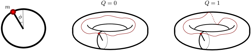
where is the angle representing the position of the particle in the ring (see Fig. 1 [left]), is its moment of inertia, and is a free parameter, analogous to the angle of QCD.
The system can also be formulated as a path integral at finite temperature and Euclidean volume via the partition function [15, 16]
| (4) |
where action and topological charge in the continuum read
| (5) |
where and periodic boundary conditions are imposed, i.e. with . Additionally, topology can be easily visualized in this model, as the periodic boundary conditions make the trajectory of the particle live on the surface of a torus (see Fig. 1 [right]), where each trajectory can be classified with an integer : if the trajectory of a configuration does not wind around the torus, it has topological charge ; if it winds once around the torus, it has .
This model can be trivially solved using the quantum mechanical formalism, and the energy levels of the system read
| (6) |
from which one can build the thermal partition function and obtain the probability distribution of each topological sector,
| (7) |
With these results one can test the order of limits of Eq. (2). Particularly, the topological susceptibility in a finite volume can be computed as
| (8) |
and studying the infinite volume limit as in Eq. (2) one finds
| (9) |
which is trivially zero. Alternatively, one can obtain the topological susceptibility in the zero temperature limit () directly from the energy spectrum in Eq. (6), which reads
| (10) |
This result can also be obtained with the conventional order of limits [14], and contradicts the result coming from the proposed order of limits in Eq. (9). In the following, we will validate the conventional order of limits using lattice simulations, for which we will need to deal with topology freezing and the sign problem.
3 Topology freezing and the winding HMC algorithm
Standard algorithms for lattice QCD, such as the Hybrid Monte Carlo (HMC) algorithm [17], are well-known to suffer from topology freezing: near the continuum limit, continuous update algorithms get trapped within a topological sector, thus failing to sample the full configuration space and leading to exponentially increasing autocorrelation times as the continuum limit is approached in a finite volume.
The topology freezing problem is also present in simple models such as the quantum rotor, making them useful testbeds for new algorithms aiming to tackle this problem. The spacetime discretization of the quantum rotor consists of angle variables for separated by a lattice spacing . Here we will work with the so-called standard discretization of the action and topological charge,
| (11) |
where , as well as with the classical perfect discretization,111Note that the classical perfect topological charge, , has a geometrical definition and is exactly an integer.
| (12) |
Note that both discretizations lead to the same continuum limit of Eq. (5) when taking along a line of constant physics with .
The simplest idea to build an algorithm that can sample topology efficiently is to find transformations between topological sectors. Such a topology-changing transformation can be easily built for the quantum rotor, for which we define the winding transformation by
| (13) |
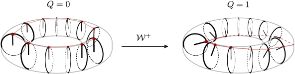
where the (winding) or (antiwinding) is common to all . As shown in Fig. 2, the transformation gradually winds the trajectory of a configuration around itself exactly once, such that . This transformation can be easily embedded into a Metropolis algorithm with acceptance
| (14) |
and we denote the combination of this Metropolis step with the HMC algorithm as the winding HMC (wHMC) algorithm [18], which restablishes ergodicity within the full configuration space if the acceptance is significant.
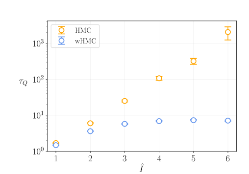
In Fig. 3 we show the scaling of autocorrelation times of the topological charge, , from simulations with the HMC and wHMC algorithms. While the autocorrelations of HMC scale exponentially, as expected, the ones of wHMC eventually saturate, thus solving the topology freezing problem in this model.
4 The sign problem and truncated polynomials
The sign problem is caused by the imaginary term in Eq. (4), which for is highly oscillatory and leads to uncertainties which grow exponentially with the volume of the system. A conventional workaround is to define so that the integrand becomes real and the system can be simulated using standard sampling algorithms. By performing simulations at different imaginary values of , one can then use the analiticity of an observable,
| (15) |
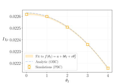
along with analytic continuation to obtain the expansion coefficients by performing fits to data. This is depicted in Fig. 4 (left), we show results of for different values of .
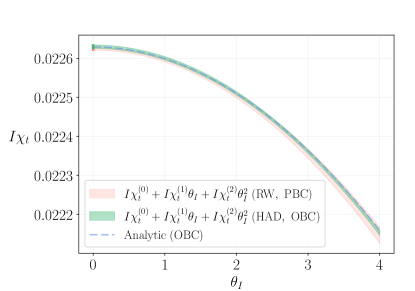
An alternative method that allows to obtain arbitrarily high derivatives of just from a single simulation at relies on the fact that a differentiable function can be Taylor expanded around . The construction of such Taylor expansion can be automatized for any arbitrarily complex function by using the algebra of truncated polynomials [19]: if is a truncated polynomial of order and we code all elementary mathematical functions of these polynomials, will be a truncated polynomial containing the first derivatives of . Truncated polynomials are a particular automatic differentiation technique and for our computations we use FormalSeries.jl [20], which can be used for any arbitrarily complicated function , such as a computer program implementing reweighting or the HMC algorithm.
A particularly simple application of truncated polynomials to extract higher order derivatives from an existing simulation at is by reweighting to via the identity
| (16) |
By replacing with the truncated polynomial with and , one automatically obtains the full analytical dependence of the Taylor expansion of with respect to up to order from a single ensemble. This is shown in Fig. 4 (right), where by reweighting a single standard simulation at with periodic boundary conditions we automatically obtain ; particularly, we see that agrees with the analytical result obtained with open boundary conditions.
| Method | ||
|---|---|---|
| Fit | 4.5238(16) | -6.08(48) |
| Reweighting | 4.52501(76) | -5.99(25) |
| HAD | 4.52604(83) | -5.980(34) |
However, a drawback of reweighting is that the denominator in Eq. (16) has disconnected contributions that are exponentially noisier with the size of the system. To solve this, one can apply the truncated polynomials directly into the HMC algorithm. Using the standard discretization of the model, the HMC equations of motion read
| (17) | ||||
where is the Hamiltonian of the system. By replacing by a truncated polynomial, , we obtain a Markov chain of samples, , that carry the derivatives with respect to , and we denote this algorithm as Hamiltonian Automatic Differentiation (HAD). The Taylor expansion of observables is obtained by the computation of conventional expectation values using the samples , and does not contain the noisy disconnected contributions of the reweighting technique.222However, the Metropolis accept-reject step is not differentiable and cannot be used with this method, so one must integrate the equations of motion with high enough precision to avoid systematic effects. In Fig. 4 (right), we show the curve obtained from a single HAD simulation, and one can appreciate that the predictions for high are more accurate than the ones obtained by reweighting. The comparison can be seen more transparently in Tab. 1, where the error of the HAD algorithm is reduced by an order of magnitude with respect to the other methods at equivalent statistics.
5 Results
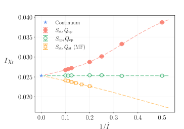
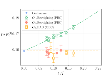
Fig. 5 (left) shows our results of a local version of the topological susceptibility, —with which the choice of boundary conditions and the quantization of the topological charge is irrelevant—from simulations with periodic boundary conditions with both the standard and classical perfect discretizations at different values of the lattice spacing. The wHMC algorithm allowed us to perform simulations very close to the continuum, and our results agree with the analytical results obtained with open boundary conditions. All choices of boundary conditions and discretization lead to the continuum result in Eq. (10), validating the conventional order of limits.
Finally, in Fig. 5 we show our results of the linear -dependence of the ground state of the spectrum for different values of the lattice spacing, which from Eq. (6) reads , obtained through the usual spectral decomposition of an interpolator with the same symmetries as the ground state. We use both reweighting and the HAD algorithm, for different choices of boundary conditions and interpolating operators, and conclude that the continuum limit agrees with the results from quantum mechanics—and disagree with the claims of Refs. [6, 7].
6 Conclusions
We have studied a recently proposed order of limits to study infinite-volume quantities which makes disappear from all physical observables of the theory. We have studied the continuum limit of the topological susceptibility and the first -dependence correction to the ground energy state of the quantum rotor, validating the conventional wisdom on the strong problem. Even though the system suffers from topology freezing and the sign problem, these were successfully overcome by the use of the wHMC algorithm and truncated polynomials. The generalization of these proposed algorithms to more complicated models is work in progress.
Acknowledgements
We acknowledge support from the Generalitat Valenciana Grant No. PROMETEO/2019/083, the European Projects No. H2020-MSCA-ITN-2019//860881-HIDDeN and No. 101086085-ASYMMETRY, and the National Project No. PID2020-113644GB-I00, as well as the technical support provided by the Instituto de Física Corpuscular, IFIC (CSIC-UV). D.A. acknowledges support from the Generalitat Valenciana Grants No. ACIF/2020/011 and No. PROMETEO/2021/083. G.C. and A.R. acknowledge financial support from the Generalitat Valenciana Grant No. CIDEGENT/2019/040.
References
- [1] C. Abel et al., Measurement of the Permanent Electric Dipole Moment of the Neutron, Phys. Rev. Lett. 124 (2020) 081803 [2001.11966].
- [2] T. Chupp, P. Fierlinger, M. Ramsey-Musolf and J. Singh, Electric dipole moments of atoms, molecules, nuclei, and particles, Rev. Mod. Phys. 91 (2019) 015001 [1710.02504].
- [3] R.D. Peccei and H.R. Quinn, Constraints imposed by conservation in the presence of pseudoparticles, Phys. Rev. D 16 (1977) 1791.
- [4] A.E. Nelson, Naturally Weak Violation, Phys. Lett. B 136 (1984) 387.
- [5] S.M. Barr, Solving the strong problem without the Peccei-Quinn symmetry, Phys. Rev. Lett. 53 (1984) 329.
- [6] W.-Y. Ai, J.S. Cruz, B. Garbrecht and C. Tamarit, Absence of CP violation in the strong interactions, 2001.07152 .
- [7] W.-Y. Ai, J.S. Cruz, B. Garbrecht and C. Tamarit, Consequences of the order of the limit of infinite spacetime volume and the sum over topological sectors for CP violation in the strong interactions, Phys. Lett. B 822 (2021) 136616.
- [8] P. de Forcrand, Simulating QCD at finite density, PoS LAT2009 (2009) 010 [1005.0539].
- [9] C. Gattringer and K. Langfeld, Approaches to the sign problem in lattice field theory, Int. J. Mod. Phys. A 31 (2016) 1643007 [1603.09517].
- [10] B. Alles, G. Boyd, M. D’Elia, A. Di Giacomo and E. Vicari, Hybrid Monte Carlo and topological modes of full QCD, Phys. Lett. B 389 (1996) 107 [hep-lat/9607049].
- [11] L. Del Debbio, H. Panagopoulos and E. Vicari, Theta dependence of SU(N) gauge theories, JHEP 08 (2002) 044 [hep-th/0204125].
- [12] L. Del Debbio, G.M. Manca and E. Vicari, Critical slowing down of topological modes, Phys. Lett. B 594 (2004) 315 [hep-lat/0403001].
- [13] ALPHA collaboration, Critical slowing down and error analysis in lattice QCD simulations, Nucl. Phys. B 845 (2011) 93 [1009.5228].
- [14] D. Albandea, G. Catumba and A. Ramos, Strong problem in the quantum rotor, Phys. Rev. D 110 (2024) 094512 [2402.17518].
- [15] N. Fjeldso, J. Midtdal and F. Ravndal, Random walks of a quantum particle on a circle, unpublished (1987) .
- [16] W. Bietenholz, R. Brower, S. Chandrasekharan and U.J. Wiese, Perfect lattice topology: The Quantum rotor as a test case, Phys. Lett. B 407 (1997) 283 [hep-lat/9704015].
- [17] S. Duane, A.D. Kennedy, B.J. Pendleton and D. Roweth, Hybrid Monte Carlo, Phys. Lett. B 195 (1987) 216.
- [18] D. Albandea, P. Hernández, A. Ramos and F. Romero-López, Topological sampling through windings, Eur. Phys. J. C 81 (2021) 873 [2106.14234].
- [19] A. Haro, Automatic differentiation tools in computational dynamical systems, unpublished (2011) .
- [20] A. Ramos, FormalSeries.jl, May, 2023. 10.5281/zenodo.7970278.