Modelling change in neural dynamics during phonetic accommodation

Abstract

Short-term phonetic accommodation is a fundamental driver behind accent change, but how does real-time input from another speaker's voice shape the speech planning representations of an interlocutor? We advance a computational model of change in phonetic representations during phonetic accommodation, grounded in dynamic neural field equations for movement planning and memory dynamics. We test the model's ability to capture empirical patterns from an experimental study where speakers shadowed a model talker with a different accent from their own. The experimental data shows vowel-specific degrees of convergence during shadowing, followed by return to baseline (or minor divergence) post-shadowing. The model can reproduce these phenomena by modulating the magnitude of inhibitory memory dynamics, which may reflect resistance to accommodation due to phonological and/or sociolinguistic pressures. We discuss the implications of these results for the relation between short-term phonetic accommodation and longer-term patterns of sound change.

Keywords: phonetic accommodation; shadowing task; neural dynamics; computational modelling; dynamical systems

Introduction

Spoken language is rarely static; when two people converse, they subtly (and sometimes not so subtly) modulate their voices in response to one another. This phonetic accommodation is a fundamental characteristic of spoken interaction, representing the ebb and flow of human communication citep(Giles, 1973; Pardo, 2006). Experimental evidence for phonetic accommodation comes from the shadowing task paradigm, which involves a speaker reading a series of words, followed by imitating a (usually pre-recorded) model talker producing the same words citep(Goldinger, 1998). This allows for the assessment of how much change occurs as a result of shadowing the model talker, while a post-test recording of the same words can be used to establish persistence of any adaptations. There is considerable evidence that speakers converge towards a model talker in the shadowing task and that listeners are also sensitive to these short-term changes citep(Goldinger, 1998; Namy et al., 2002; Shockey et al., 2004; Tilsen, 2009). While accommodation is often cast as an automatic process citep(Goldinger, 1998), citetBabel (2012) finds that accommodation is socially-mediated, with the degree of adaptation based on the perceived social characteristics of the model talker.

Phonetic accommodation is short-term, but its accumulation over time is a key driver of accent change. Accent change generally slows significantly during adulthood, but change nonetheless can occur, especially with increased exposure to different accents citep(Evans & Iverson, 2007; Harrington et al., 2019). Exemplar models of speech processing hypothesize a mechanism behind these changes, such that the phonetic representations used in speech production are influenced by stored instances of language from speech perception citep(Gubian et al., 2023; Johnson, 2007; Pierrehumbert, 2002). In this sense, hearing another talker creates an episodic memory trace, which exerts a small bias on subsequent speech production. It stands to reason that over many such instances, small accent changes could occur, and this process of change would become accelerated if spread across a community.

The aim of this study is to develop a computational model of neural dynamics during real-time phonetic imitation. Previous models of phonetic imitation are largely exemplar-based; for example, citetGoldinger (1998) models data from a shadowing task using Minerva2 citep(Hintzman, 1984, 1986). We take inspiration from this work, but advance a new direction using dynamic neural field models of movement planning citep(Schöner et al., 2016), which incorporate exemplar-like dynamics using a biophysically-plausible model of the coupling between perception, memory and speech planning citep(Gafos, 2006; Tilsen, 2009). A strong motivation for this approach is that complex motor synergies are hypothesized to represent the locus of speech planning citep(Fowler, 1980; Kelso et al., 1986), and dynamic field models are already well-developed for auditory-motor dynamics underlying production and perception citep(Gafos, 2006; Roon & Gafos, 2016; Stern & Shaw, 2023; Tilsen, 2019, 2022). We first report the results of an experiment where speakers shadowed a model talker with an accent different from their own. This is followed by a dynamic neural field model, which can capture various properties of the experimental data, with inhibitory memory dynamics corresponding to degrees of phonetic accommodation.

Experimental study

Experiment design

We report an experimental study of phonetic accommodation in a shadowing task, which involves speakers of Northern Anglo British English shadowing a model talker with an accent different from their own. The experiment featured three blocks: pre-test, shadowing and post-test citep(Babel, 2010; Goldinger, 1998). In the pre-test and post-test blocks, speakers read aloud single word productions in hVd format, along with a set of target words. The shadowing block then required subjects to identify and repeat the same target words produced by a model talker, who was a male Standard Southern British English speaker aged 21 at the time of recording. In this study, we specifically focus on two vowels that differ substantially between the experimental participants and model talker: bath and strut. Standard Southern British English realizes these vowels as [A] and [2] respectively, while in almost all varieties of Northern Anglo English these vowels are produced as [a] and [U]. These vowels represent the most characteristic difference between northern and southern varieties in England citep(Wells, 1982); they are highly salient to listeners and can also undergo change as a consequence of long-term different-accent exposure citep(Evans & Iverson, 2007). The bath target words were bath, chance, fast, mast, staff, while the strut words were strut, bust, chuck, fun, mud. Another 10 non-bath/strut words were also included in all experimental blocks as distractor stimuli.

Participants and recording

All participants were first-language speakers of Northern Anglo English, aged between 19–22 years old. 18 speakers completed the experiment, with 13 speakers (11 female, 2 male) included in the analysis (two speakers were removed as they recognized the model talker, and three speakers were removed due to significant distortion in the audio recordings). The experiment was adminstered using PsychoPy citep(Peirce et al., 2019), with audio recorded in a sound-attenuated booth at 44.1 kHz using a Beyerdynamic Opus 55 headset microphone (5cm from the mouth), pre-amplified and digitized using a Sound Devices USBPre 2 audio interface. Audio stimuli were delivered using Beyerdynamic DT 770 headphones.

Data processing

All recordings were automatically force-aligned using Montreal Forced Aligner citep(McAuliffe et al., 2017). Formants were estimated using the FastTrack algorithm citep(Barreda, 2021), which obtains accurate formant measurements by optimizing over LPC formant analysis settings. We specifically use the Python implementation of FastTrack citep(Fruehwald & Barreda, 2023), whereby we optimize the estimation of $F_{n\in\{1,2,3,4\}}$ formant trajectories using a 20-step search window of 4000–7000 Hz, with 25 ms window length, 2 ms step size, 50 Hz pre-emphasis, and 5th-order DCT smoothing of trajectories. Formant values were subsequently extracted from the temporal midpoint of each vowel and by-speaker $z$-scored across all hVd and target words citep(Babel, 2012). The degree of accommodation was quantified by calculating the Euclidean distance $d$ between each speaker's production ($spk$) and the corresponding model talker production ($mod$) as in (1).

$$d(\text{mod, spk})=\sqrt{(F_{1\text{mod}}-F_{1\text{spk}})^{2}+(F_{2\text{mod}}-F_{2\text{spk}})^{2}}$$ (1)

We subtract the value of $d(\text{mod, spk})$ for the baseline block from the shadowing and post-test blocks in order to calculate a `difference in distance' metric that captures the degree of accommodation citep(Babel, 2012). Values of zero indicate no accommodation, negative values indicate convergence (reduced distance from the model talker), and positive values indicate divergence (increased distance from the model talker). All data processing and analysis was carried out in the Python programming language, using the packages NumPy citep(Harris et al., 2020), Pandas citep(The pandas development team, 2020) and plotnine citep(The plotnine development team, 2025).

Results

We fit four Bayesian linear mixed models to the difference in distance ($d$) values for each combination of task (shadowing/post) and vowel (bath/strut). Each model contains a grand intercept $\mu$ and random intercepts $b_{\text{word}}$ and $b_{\text{speaker}}$. Models were written in Stan and run using cmdstanpy citep(Stan Development Team, 2024) with weakly informative priors $\mu\sim\mathcal{N}(0,2)$ and $b\sim\mathcal{N}(0,1)$, using 4 MCMC chains, 500 warmup iterations, and 2000 sampling iterations. Table 1 suggests that, on average, speakers accommodate to the model talker during the shadowing task, but strut shows more than triple the amount of convergence ($\bar{d}=-0.25$) than bath ($\bar{d}=-0.08$). The vowels differ only minimally post-shadowing, with bath slightly diverging from the model talker post-shadowing ($\bar{d}=0.03$), while strut is closer to the pre-shadowing baseline ($\bar{d}=0.01$).

Table 1: Difference in distance for bath, strut vowels in shadowing and post-shadowing blocks. Values are $z$-scores.

vowel	task	$\bar{d}$	95% CI
bath	shadow	$-$0.08	[$-$0.30, 0.15]
	post	0.03	[$-$0.22, 0.25]
strut	shadow	$-$0.25	[$-$0.60, 0.13]
	post	0.01	[$-$0.19, 0.16]

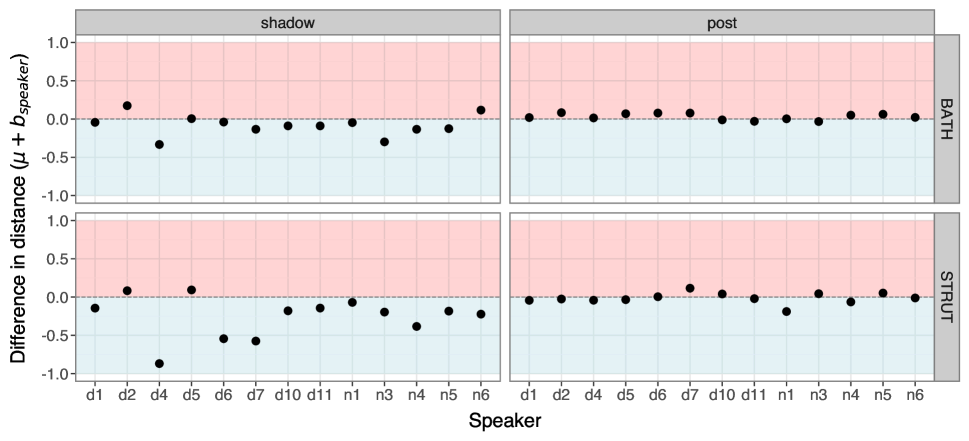
Figure 1: By-speaker difference in distance values for vowel and block. Values are from the Bayesian model and represent each speaker's random intercept coefficient added to the model's grand intercept. Negative values indicate convergence towards the model talker (blue shading); positive values indicate divergence (red shading); zero values indicate no accommodation. Speaker labels (d/n) refer to data collected by different experimenters and do not reflect any differences in speaker characteristics.

The 95% credible intervals in Table 1 point towards extensive between-speaker variation, with a wide range of compatible values for the true mean. Figure 1 shows speaker-specific difference in distance values. These values represent the fitted by-speaker random intercepts, added to the model's grand intercept, which provides an estimate of each speaker's difference in distance value. The plot reflects the overall trend of some convergence in bath, with the majority of speakers below the zero line, followed by the majority of speakers showing a small amount of divergence post-shadowing. However, some speakers do show small divergence during shadowing, such as d7 and n6, but all speakers are very close to baseline or above post-shadowing. The strut data is more variable during shadowing, with some speakers showing substantial convergence to the model talker (e.g. d4, d6, d7). Two speakers diverge during shadowing for strut (d2, d5), one of whom also diverged for bath (d2). Finally, the post-shadowing strut data shows strong clustering around the zero line, indicating a return to the pre-shadowing baseline production. Speaker n1 is the only one who is slightly closer to the model talker post-shadowing than during shadowing, but these differences remain small.

Summary and next steps

The overall picture from this sample is considerable variability in accommodation, with greater mean convergence in strut. Both vowels show minor amounts of divergence in post-shadowing, with bath showing slightly greater divergence. Why do these vowels tend to show different patterns of accommodation? One explanation is that speakers possess greater awareness of accent differences in some vowels than others citep(Babel, 2010). citetEvans & Iverson (2007) report similar results in a longitudinal study of accent change in young northern speakers exposed to Standard Southern British English (SSBE). They find that strut converges to the SSBE variant to a greater extent than bath over a period of two years, which the authors suggest is due to greater salience of bath in northern English. We find a similar pattern in response to a single SSBE-accented production, which suggests that strut may be more susceptible to change than bath. We address a potential mechanism behind these results in the following sections, where we outline a computational model of phonetic accommodation.

Neural field model of phonetic accommodation

Any model of phonetic accommodation minimally requires an account of (1) real-time dynamics of speech planning and the factors that shape planning; (2) the persistence of these dynamics in short-term memory. A promising candidate in this respect is the class of dynamic field models of movement planning citep(Erlhagen & Schöner, 2002), which are inspired by a long history of research in synergetics, self-organization and neural information processing citep(e.g. Grossberg, 1980; Haken, 1977; Kelso, 1995). A dynamic neural field (DNF) functionally represents a neural population that is sensitive to a perceptual or movement parameter dimension, and a DNF's evolution is shaped by inputs to the field, such as perceptual and task-related input, as well as memory dynamics and intrinsic dynamical mechanisms, such as self-excitation. See citetSchöner et al. (2016) for a tutorial introduction and examples of different applications across the cognitive sciences.

Dynamic neural fields are relatively well developed as models of the neural dynamics underpinning speech planning, execution and perception citep(e.g. Gafos, 2006; Kirkham & Strycharczuk, 2024; Roon & Gafos, 2016; Stern & Shaw, 2023; Tilsen, 2007, 2019). Specifically, DNFs facilitate coupling between perceptual, motor and memory fields citep(Erlhagen & Schöner, 2002), which is particularly important for multi-dimensional representations that change with experience. In the sections below, we outline a minimal DNF model architecture for phonetic planning and memory in speech production, followed by simulations of change in the neural planning dynamics that could underpin phonetic accommodation.

Model architecture

A dynamic neural field (DNF) evolves according to the citetAmari (1977) model that underpins Equation (2):

$$\tau\dot{u}(x,t)=-u(x,t)+h+c_{\text{memory}}u_{\text{memory}}(x,t)\\ +c_{\text{auditory}}s_{\text{auditory}}(x,t)+c_{\text{response}}s_{\text{response}}(x,t)\\ +\int k(x-x^{\prime})g(u(x^{\prime},t))dx^{\prime}+q\xi(x,t)$$ (2)

where $\tau$ dictates the rate of field evolution, $-u(x,t)$ is time-dependent activation at each field site $x$, $h$ is the resting level of the neural field, $s(x,t)$ represents an input to the field, and $\xi(x,t)$ is Gaussian noise scaled by a coefficient $q$ citep(Schöner et al., 2016). As we are dealing with acoustic measurements, we assume that $x$ represents a one-dimensional reduction of the $F1\sim F2$ acoustic feature space, but a more realistic model could capture the coupling between acoustic, perceptual and articulatory representations using a multi-layer model.

Inputs $s(x,t)$ are Gaussian distributions over a parameter $x$ with amplitude $a$, centroid $p$ and width $w$,

$$s(x,t)=\sum_{i}a_{i}\exp\left[-\frac{(x-p_{i})^{2}}{2w^{2}_{i}}\right].$$ (3)

Response input $s_{\text{response}}(x,t)$ represents retrieval of a speech planning representation in response to the experiment's visual prompt and is weighted by $c_{\text{response}}$. We model this as retrieval of the appropriate representation from long-term memory citep(Roon & Gafos, 2016) and do not incorporate any competitive selection dynamics citep(e.g. Tilsen, 2019). Auditory input $s_{\text{auditory}}(x,t)$ is an auditory-perceptual input that couples the model talker's production to activation dynamics with strength $c_{\text{auditory}}$. We here treat $c_{\text{auditory}}$ as capturing the degree of attention to the incoming speech, which we expect is very high during a shadowing task, but lower in normal conversational interaction. In the shadowing block, auditory input cues the response input, whereas in the non-shadowing block the response is cued by a visual prompt (although we do not explicitly model the visual cue in this study).

The interaction kernel $k(x-x^{\prime})$ in (4) specifies excitatory and inhibitory forces across the activation field.

$$k(x-x^{\prime})=\frac{c_{\text{excite}}}{\sqrt{2}\pi\sigma_{\text{excite}}}\exp\left[-\frac{(x-x^{\prime})^{2}}{2\sigma^{2}_{\text{\text{excite}}}}\right]\\ -\frac{c_{\text{inhibit}}}{\sqrt{2}\pi\sigma_{\text{inhibit}}}\exp\left[-\frac{(x-x^{\prime})^{2}}{2\sigma^{2}_{\text{inhibit}}}\right]-c_{\text{global}}$$ (4)

Each field location only contributes to above-threshold activation when it exceeds a threshold of $u=\alpha$, where typically $\alpha=0$. Interaction generates local excitation and lateral inhibition, meaning that activation close to an input's centroid will be excited, whereas more distal activation will be inhibited. $c_{\text{excite}}$, $c_{\text{inhibit}}$ and $\sigma_{\text{excite}}$, $\sigma_{\text{inhibit}}$ are the mean and standard deviation of the excitatory/inhibitory components, and $c_{\text{global}}$ is a global inhibition constant.

The interaction kernel is gated by a sigmoidal function

$$g(u)=\frac{1}{1+\exp(-\beta(u-\alpha))}$$ (5)

where $\beta$ is the slope of the sigmoid and $\alpha$ is a threshold value of $u$ (typically 0).

Short-term memory dynamics are achieved by a Hebbian layer citep(Samuelson et al., 2011). This is represented by the memory field $u_{\text{memory}}(x,t)$ in (6) coupled to $u(x,t)$ with strength $c_{\text{memory}}$ and is subject to local interactions $w(x-x^{\prime})$.

$$\dot{u}_{\text{mem}}(x,t)=\begin{cases}\frac{1}{\tau_{\text{mem}}}[-u_{\text{mem}}(x,t)\\ +\int w(x-x^{\prime})g(u(x^{\prime},t))dx^{\prime}],&g(u)>\alpha\\[10.00002pt] \frac{1}{\tau_{\text{decay}}}[-u_{\text{mem}}(x,t)],&g(u)\leq\alpha\end{cases}$$ (6)

When activation in the primary field $u(x,t)$ is greater than threshold $\alpha$ the sigmoid $g(u)$ gates activation into the memory field at a rate determined by $\tau_{\text{mem}}$. When $g(u)\leq\alpha$ memory at those field locations undergoes decay at a rate of $\tau_{\text{decay}}$. The memory field evolves on a slower timescale than the field dynamics, while memory decay evolves the slowest, such that $\tau_{\text{decay}}>\tau_{\text{mem}}>\tau$. This reflects the fact that memory formation happens faster than memory decay. Note that in our simulations we use an interaction kernel for both the main parameter field $k(x-x^{\prime})$ and the memory field $w(x-x^{\prime})$. The memory kernel is specified for local inhibition but not global inhibition for reasons we discuss in the following sections.

Simulating interaction

A simulated interaction proceeds as follows in three blocks.

1. Baseline. The visual prompt cues $s_{\text{response}}(x,t)$ input, which raises activation above threshold and triggers production at the parameter value corresponding to peak activation. We assume $s_{\text{auditory}}(x,t)=0$ during the baseline block, meaning it has no influence on activation. The field dynamics leave an activation trace in $u_{\text{memory}}(x,t)$.

2. Shadowing. Auditory input from the model talker $s_{\text{auditory}}(x,t)>0$ raises sub-threshold activation in $u(x,t)$ and the response input $s_{\text{response}}(x,t)$ subsequently raises activation above threshold and production occurs. High attention to the model talker reflected in a large $c_{\text{auditory}}$ value means that input amplitude is high, which causes its effects to persist over time. These dynamics leave an activation trace in the updated $u_{\text{memory}}(x,t)$ field.

3. Post-shadowing. The visual prompt cues $s_{\text{response}}(x,t)$, while $s_{\text{auditory}}(x,t)$ = 0, which raises activation above threshold, cues production, and leaves a memory trace.

All simulations were implemented in the Python programming language using NumPy citep(Harris et al., 2020) and SciPy citep(Virtanen et al., 2020), with visualizations made using Matplotlib citep(Hunter, 2007). Numerical solutions to differential equations were calculated using an Explicit Runge-Kutta method of order 5(4) via SciPy's integrate.solve_ivp function.

Short-term change in phonetic representations

We assume independent DNFs for bath and strut, so we use the same initialization for both vowels, centring the idealized speaker's memory trace at zero across a field comprising $x\in[-10,+10$] (the majority of the field either side of zero is subject to significant inhibition, so it is unlikely that such areas receive any significant activation). The inputs $s_{\text{auditory}}(x,t)$ are based on the average $z$-scored distance from the model talker, with strut $=-1.4$ and bath $=-1.2$. These input values represent differences from the idealized speaker's existing representation, which has a mean of 0.

The planning field interaction kernel $k(x-x^{\prime})$ is defined as $c_{\text{excite}}=2,\sigma_{\text{excite}}=0.2,c_{\text{inhibit}}=1,\sigma_{\text{inhibit}}=2,c_{\text{global}}=0.5$. The default memory kernel $w(x-x^{\prime})$ is identical to the field kernel, except $c_{\text{global}}=0$ and $\sigma_{\text{excite}}=0.1$. Temporal parameters are $\tau=25$, $\tau_{\text{memory}}=150$, $\tau_{\text{decay}}=500$, while $c_{\text{memory}}=10$, $c_{\text{auditory}}=10$, $c_{\text{response}}=1$, $h=-2$, $q=3$, $\beta=1.5$. All inputs $s(x,t)$ have $a=10$ and $w=0.5$.

All simulations lasted for a duration of 300 ms. Inputs are constant over time because we make the assumption that monophthongs are one-target vowels citep(Strycharczuk et al., 2024). To represent the acoustic parameter selected for speech production, we sample at the time-step corresponding to peak activation, with the $x$-location of peak activation representing the selected parameter value for production.

We first initialize short-term memory $u_{\text{memory}}(x,t)$ as a zero-valued flat field and then run simulations with a single input $a=100,p=0,w=0.5$, which when coupled to the memory field serves to update $u_{\text{memory}}(x,t)$ based on the resulting field activation. This represents the existing short-term memory for each vowel, while the response input $s_{\text{response}}(x,t)$ is drawn from longer-term phonological memory. For each simulation, the initial memory state is the memory state at the end of the previous simulation.

Phonetic convergence and return to baseline

Our simulations show that the model straightforwardly captures the dynamics of phonetic convergence followed by return to near-baseline. In the strut vowel simulations, peak activation is at $x=-0.22$ during shadowing and $x=0.02$ during post-shadowing. This is close to the empirical means of $\bar{d}=-0.25$ and $\bar{d}=0.01$, with a relative difference between shadowing and post-shadowing of $\bar{d}_{\text{diff}}=0.26$ and $x_{\text{diff}}=0.24$, which represents very good agreement between model and data.

The occurrence of accommodation during shadowing versus return to (near) baseline post-shadowing is a consequence of the auditory input and inhibitory dynamics. This is shown in Figure 2 (top), where the small bump at the left of the activation field during shadowing (orange line) represents the effects of $s_{\text{auditory}}(x,t)$. While this input does not reach the activation threshold of 0, it does slightly pull the activation centroid leftwards, resulting in the small degree of observed accommodation towards the model talker. The degree of accommodation is attenuated as the input occurs in a region of parameter space that is subject to considerable inhibition (i.e. the negative values near the base of the primary activation peak). This small amount of accommodation has a very minimal effect on the memory field in Figure 2 (bottom), with an almost undetectable rightwards shift of the memory peak as a consequence of greater inhibition in short-term memory. The memory field evolves more slowly than the parameter activation field, meaning that any production effects are very gradual. Note that while these effects are very small, they reflect the empirical changes in speech production as a consequence of minimal short-term exposure to the model talker.

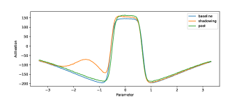
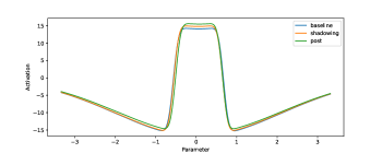
Figure 2: Activation field (top) and memory field (bottom) for strut simulations. The $x$ parameter range has been truncated to highlight small differences in the activation peaks.

Phonetic convergence followed by divergence

The previous section modelled convergence followed by return to baseline, but both vowels also show small amounts of divergence in the post-shadowing block, which is on average larger for bath. Despite the small average magnitude of divergence, Figure 1 also shows that some speakers diverge more than others, so we now model this phenomenon with a focus on replicating the average effect for bath.

In order to model accommodation followed by subsequent phonetic divergence, we turn to differences in the memory kernel parameters, which situates the differences between bath and strut in vowel-specific memory dynamics, rather than purely metric parameter differences. We run the same simulation as for strut but with three changes. First, $s_{\text{auditory}}(x,t)$ has $p=-1.2$ rather than $p=-1.4$ to reflect the empirical baseline distance from the model talker for bath. Second, the memory kernel has higher local inhibition, with $c_{\text{inhibit}}=1.8$ (compared to $c_{\text{inhibit}}=1$ for strut). Third, the memory kernel also has higher $\sigma_{\text{inhibit}}=3$ (compared with $\sigma_{\text{inhibit}}=2$ for strut). This specifies the memory kernel for bath as having stronger and wider local inhibition, which we interpret as corresponding to the memory field's increased resistance to the input. This is in line with previous literature showing that bath is more resistant to accommodation than strut for northern speakers.

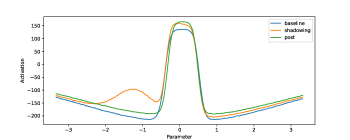
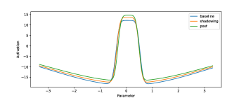
Figure 3: Activation field (top) and memory field (bottom) for bath simulations. The $x$ parameter range has been truncated to highlight small differences in the activation peaks.

The resulting simulations for bath show peak activation values at $x=-0.1$ for shadowing and $x=0.02$ for post-shadowing, which is close to the mean empirical magnitude of accommodation ($\bar{d}=-0.08$) and divergence ($\bar{d}=0.03$). If we take the relative difference between shadowing and post-shadowing then $\bar{d}_{\text{diff}}=0.11$ and $x_{\text{diff}}=0.12$, showing very good agreement between model and data. Figure 3 shows this pattern, where the sub-threshold auditory input peak on the left-hand side (orange line) pulls the activation peak slightly leftwards, representing accommodation, but inhibitory memory dynamics repel this slightly and the subsequent post-shadowing production is shifted slightly rightwards, representing divergence. Note that the peaks are narrower due to the fact that the bath $s_{\text{auditory}}(x,t)$ input is closer to the existing activation peak than strut. Also note that the differences between conditions in the memory trace are slightly larger than those in Figure 2, as a consequence of stronger inhibitory dynamics in the memory field for bath.

Discussion

Northern Anglo English speakers show vowel-specific patterns of accommodation to a Standard Southern British English model talker during a shadowing task. These differences are in agreement with previous research, whereby strut changes more readily than bath. A dynamic neural field model accurately captures these dynamics of adaptation and short-term memory, suggesting that the observed differences between strut and bath can be modelled as differences in the magnitude of inhibitory dynamics in short-term memory.

The fact that bath has stronger inhibition in memory than strut is a good fit to the data, while inhibitory dynamics are also a well-documented characteristic of speech production citep(Stern & Shaw, 2023; Tilsen, 2019), but what is the explanation for vowel-specific differences in memory? We propose two potential explanations. The first is phonological; namely that convergence in bath would have structural implications for northern speakers, whose vowel in the palm/start lexical sets is phonetically similar to SSBE bath. Any convergence would, therefore, lead to potential merger between these vowel categories, so the greater inhibition may exist to prevent category merger. A second explanation is sociolinguistic. Previous research suggests that the bath vowel is a strong shibboleth of the north/south divide citep(Wells, 1982) and northern speakers tend to show resistance to change in this vowel citep(Evans & Iverson, 2007). Our empirical data shows that these inhibitory dynamics are not sufficient to completely block accommodation, which suggests an automatic dimension to accommodation citep(Goldinger, 1998). However, the inhibitory dynamics do attenuate the magnitude of accommodation and trigger divergence in short-term memory, which bolsters the maintenance of this salient accent feature.

In the present study, we have only modelled the average effects from the statistical model, but varying degrees of accommodation and persistence can also be modelled through variation in the input weighting (i.e. reflecting attention to the model talker) and in the kernel parameters, which reflect excitatory and inhibitory forces. The interaction kernel captures the stability and resilience of short-term representations, so variation in these parameters is a potential locus of speaker-specific variation, which could explain differences in adaptation. For example, reducing the inhibitory component of the memory kernel for bath produces a return closer to the baseline production, rather than a dissimilatory effect.

In future work we hope to make a number of advances on the current model. First, a more realistic model of phonetic accommodation necessarily requires an account of bidirectional influence between interacting speakers, as well as the role of lexical competition in sound change citep(Wedel, 2012). Second, we aim to develop better models of how speech planning representations, which are hypothesized to reside in low-dimensional articulatory parameters citep(Browman & Goldstein, 1992), are coupled to acoustic parameters. This would allow for the generation of acoustic parameters from nonlinear gestural models of articulatory control, and vice versa citep(Kirkham, 2025; Sorensen & Gafos, 2016; Stern & Shaw, 2024).

Conclusion

We demonstrate that vowel-specific phonetic accommodation can be modelled as differences in short-term inhibitory memory dynamics, which we hypothesize is motivated by phonological contrast and socially-motivated resistance to change. Vowels with weaker inhibitory dynamics are predicted to undergo greater accommodation, which if repeated over many interactions could lead to long-term patterns of sound change.

References

- Amari (1977) Amari, S.-i. (1977). Dynamics of pattern formation in lateral-inhibition type neural fields. Biological Cybernetics, 27(2), 77–87.
- Babel (2010) Babel, M. (2010). Dialect divergence and convergence in New Zealand English. Language in Society, 39(4), 437–456.
- Babel (2012) Babel, M. (2012). Evidence for phonetic and social selectivity in spontaneous phonetic imitation. Journal of Phonetics, 40(1), 177-189.
- Barreda (2021) Barreda, S. (2021). Fast Track: Fast (nearly) automatic formant-tracking using Praat. Linguistics Vanguard, 7(1), 20200051.
- Browman & Goldstein (1992) Browman, C. P., & Goldstein, L. (1992). Articulatory phonology: an overview. Phonetica, 49(3-4), 155–180.
- Erlhagen & Schöner (2002) Erlhagen, W., & Schöner, G. (2002). Dynamic field theory of movement preparation. Psychological Review, 109(3), 545–572.
- Evans & Iverson (2007) Evans, B. G., & Iverson, P. (2007). Plasticity in vowel perception and production: A study of accent change in young adults. Journal of the Acoustical Society of America, 121(6), 3814–3826.
- Fowler (1980) Fowler, C. A. (1980). Coarticulation and theories of extrinsic timing. Journal of Phonetics, 8(1), 113–133.
- Fruehwald & Barreda (2023) Fruehwald, J., & Barreda, S. (2023). fasttrackpy. Zenodo. Retrieved from https://doi.org/10.5281/ZENODO.10212099
- Gafos (2006) Gafos, A. I. (2006). Dynamics in grammar. In L. Goldstein, D. Whalen, & C. T. Best (Eds.), Laboratory phonology 8: Varieties of phonological competence (pp. 51–79). Berlin: Mouton de Gruyter.
- Giles (1973) Giles, H. (1973). Accent mobility: A model and some data. Anthropological Linguistics, 15(2), 87–105.
- Goldinger (1998) Goldinger, S. D. (1998). Echoes of echoes? an episodic theory of lexical access. Psychological Review, 105(2), 251–279.
- Grossberg (1980) Grossberg, S. (1980). Biological competition: Decision rules, pattern formation, and oscillations. Proceedings of the National Academy of Sciences, 77(4), 2338–2342.
- Gubian et al. (2023) Gubian, M., Cronenberg, J., & Harrington, J. (2023). Phonetic and phonological sound changes in an agent-based model. Speech Communication, 147, 93–115.
- Haken (1977) Haken, H. (1977). Synergetics: An introduction. Berlin: Springer-Verlag.
- Harrington et al. (2019) Harrington, J., Gubian, M., Stevens, M., & Schiel, F. (2019). Phonetic change in an Antarctic winter. Journal of the Acoustical Society of America, 146(5), 3327–3332.
- Harris et al. (2020) Harris, C. R., Millman, K. J., van der Walt, S. J., Gommers, R., Virtanen, P., Cournapeau, D., … Oliphant, T. E. (2020). Array programming with NumPy. Nature, 585(7825), 357–362.
- Hintzman (1984) Hintzman, D. L. (1984). Minerva 2: A simulation model of human memory. Behavior Research Methods, Instruments, & Computers, 16(1), 96–101.
- Hintzman (1986) Hintzman, D. L. (1986). ``Schema abstraction" in a multiple-trace memory model. Psychological Review, 93(4), 411–428.
- Hunter (2007) Hunter, J. D. (2007). Matplotlib: A 2D graphics environment. Computing in Science & Engineering, 9(3), 90–95.
- Johnson (2007) Johnson, K. (2007). Decisions and mechanisms in exemplar-based phonology. In M.-J. Solé, P. S. Beddor, & M. Ohala (Eds.), Experimental approaches to phonology (pp. 25–40). Oxford: Oxford University Press.
- Kelso (1995) Kelso, J. S. (1995). Dynamic patterns: The self-organization of brain and behavior. Cambridge, MA: MIT Press.
- Kelso et al. (1986) Kelso, J. S., Saltzman, E. L., & Tuller, B. (1986). The dynamical perspective on speech production: data and theory. Journal of Phonetics, 14(1), 29–59.
- Kirkham (2025) Kirkham, S. (2025). Scaling laws for nonlinear dynamical models of articulatory control. JASA Express Letters, 5(2), 1–7.
- Kirkham & Strycharczuk (2024) Kirkham, S., & Strycharczuk, P. (2024). A dynamic neural field model of vowel diphthongisation. Proc. ISSP 2024 – 13th International Seminar on Speech Production, 193–196.
- McAuliffe et al. (2017) McAuliffe, M., Socolof, M., Mihuc, S., Wagner, M., & Sonderegger, M. (2017). Montreal Forced Aligner: Trainable text-speech alignment using Kaldi. In Proc. Interspeech 2017 (pp. 498–502).
- Namy et al. (2002) Namy, L. L., Nygaard, L. C., & Sauerteig, D. (2002). Gender differences in vocal accommodation: The role of perception. Journal of Language and Social Psychology, 21(4), 422–432.
- Pardo (2006) Pardo, J. S. (2006). On phonetic convergence during conversational interaction. Journal of the Acoustical Society of America, 119(4), 2382–2393.
- Peirce et al. (2019) Peirce, J., Gray, J. R., Simpson, S., MacAskill, M., Höchenberger, R., Sogo, H., … Lindeløv, J. K. (2019). PsychoPy2: experiments in behavior made easy. Behavior Research Methods, 51(1), 195–203.
- Pierrehumbert (2002) Pierrehumbert, J. B. (2002). Word-specific phonetics. In C. Gussenhoven & N. Warner (Eds.), Laboratory phonology 7 (pp. 101–139). Berlin: Mouton de Gruyter.
- Roon & Gafos (2016) Roon, K. D., & Gafos, A. I. (2016). Perceiving while producing: Modeling the dynamics of phonological planning. Journal of Memory and Language, 89(2), 222–243.
- Samuelson et al. (2011) Samuelson, L. K., Smith, L. B., Perry, L. K., & Spencer, J. P. (2011). Grounding word learning in space. PLoS ONE, 6(12), e28095.
- Schöner et al. (2016) Schöner, G., Spencer, J. P., & The DFT Research Group. (2016). Dynamic thinking: A primer on dynamic field theory. Oxford: Oxford University Press.
- Shockey et al. (2004) Shockey, K., Sabadini, L., & Fowler, C. A. (2004). Imitation in shadowing words. Perception & Psychophysics, 66(3), 422–429.
- Sorensen & Gafos (2016) Sorensen, T., & Gafos, A. I. (2016). The gesture as an autonomous nonlinear dynamical system. Ecological Psychology, 28(4), 188–215.
- Stan Development Team (2024) Stan Development Team. (2024). Stan Reference Manual, v2.36.0. https://mc-stan.org.
- Stern & Shaw (2023) Stern, M. C., & Shaw, J. A. (2023). Neural inhibition during speech planning contributes to contrastive hyperarticulation. Journal of Memory and Language, 132(104443), 1–16.
- Stern & Shaw (2024) Stern, M. C., & Shaw, J. A. (2024). Towards a minimal dynamics for gestures: A law relating velocity and position. Proc. ISSP 2024 – 13th International Seminar on Speech Production, 262–265.
- Strycharczuk et al. (2024) Strycharczuk, P., Kirkham, S., Gorman, E., & Nagamine, T. (2024). Towards a dynamical model of English vowels: Evidence from diphthongisation. Journal of Phonetics.
- The pandas development team (2020) The pandas development team. (2020). pandas-dev/pandas: Pandas. https://doi.org/10.5281/zenodo.3509134.
- The plotnine development team (2025) The plotnine development team. (2025). plotnine: A grammar of graphics for Python. https://doi.org/10.5281/zenodo.1325308.
- Tilsen (2007) Tilsen, S. (2007). Vowel-to-vowel coarticulation and dissimilation in phonemic-response priming. UC Berkeley Phonology Lab Annual Report, 3(1), 416–458.
- Tilsen (2009) Tilsen, S. (2009). Subphonemic and cross-phonemic priming in vowel shadowing: Evidence for the involvement of exemplars in production. Journal of Phonetics, 37(3), 276–296.
- Tilsen (2019) Tilsen, S. (2019). Motoric mechanisms for the emergence of non-local phonological patterns. Frontiers in Psychology, 10(2143), 1–25.
- Tilsen (2022) Tilsen, S. (2022). An informal logic of feedback-based temporal control. Frontiers in Human Neuroscience, 16(851991), 1–29.
- Virtanen et al. (2020) Virtanen, P., Gommers, R., Oliphant, T. E., Haberland, M., Reddy, T., Cournapeau, D., … SciPy 1.0 Contributors (2020). SciPy 1.0: Fundamental Algorithms for Scientific Computing in Python. Nature Methods, 17, 261–272.
- Wedel (2012) Wedel, A. (2012). Lexical contrast maintenance and the organization of sublexical contrast systems. Language and Cognition, 4(4), 319–355.
- Wells (1982) Wells, J. C. (1982). Accents of English: Volumes 1–3. Cambridge: Cambridge University Press.