Noether Symmetries in $f\left(Q\right)-$Cosmology

Abstract

We apply the Noether symmetry analysis in $f\left(Q\right)$-Cosmology to determine invariant functions and conservation laws for the cosmological field equations. For the FLRW background and the four families of connections, it is found that only power-law $f\left(Q\right)$ functions admit point Noether symmetries. Finally, exact and analytic solutions are derived using the invariant functions.

I Introduction

Symmetric teleparallel theory of gravity Nester:1998mp and its generalizations fq1 ; fq2 ; fq3 ; fq5 ; sc1 ; gg1 ; gg2 ; gg22 ; gg3 ; gg4 ; gg5 have recently drawn the attention of cosmologists, as it provides a new geometric approach for describing cosmic acceleration and cosmic structure. In symmetric teleparallel theory, the geometry of the physical metric is non-Riemannian, and the autoparallels are independent of the metric tensor. Specifically, the connection is defined to be symmetric and flat, differing from the Levi-Civita connection. Thus, the connection introduces geometrodynamical degrees of freedom in the gravitational model. These new degrees of freedom lead to novel behaviors in the evolution of physical parameters, allowing for new physics. Cosmological applications of symmetric teleparallel theory, where dark energy is interpreted as a geometric phenomenon, can be found in cc1 ; cc2 ; cc3 ; cc4 ; cc5 ; cc6 ; cc7 ; cc8 ; cc9 . Additionally, studies on compact astrophysical objects are presented in cc10 ; cc11 ; cc12 ; cc13 ; cc14 . For a recent review of symmetric teleparallel theory, we refer the reader to revh .

In this work, we focus on studying the cosmological field equations in $f\left(Q\right)$-gravity fq1 ; fq2 . In symmetric teleparallel $f\left(Q\right)$-gravity, the gravitational Action Integral is defined by an arbitrary function $f$ of the nonmetricity scalar $Q$. When $f$ is a linear function, the Symmetric Teleparallel Equivalent to General Relativity (STEGR) theory is recovered Nester:1998mp . This gravitational theory belongs to the same family of nonlinear $f$-theories fr1 ; fr2 ; fr3 ; ft1 ; ft2 proposed for the Ricci scalar and the torsion scalar. For an extensive review on $f(R)$ theories, check sot1 ; sot2 , while for $f(T)$ theory, check Bahamonde:2021gfp . The geometrodynamical degrees of freedom in $f\left(Q\right)$-gravity can be associated with scalar fields mini , and the field equations admit a minisuperspace description. Consequently, the method of variational symmetries can be applied to analyze the integrability properties of the field equations.

The Noether symmetry analysis is a powerful technique for determining conservation laws for nonlinear differential equations derived from a variational principle. Specifically, we identify the function $f\left(Q\right)$ for which the field equations admit variational symmetries. Using Noether’s theorem, we construct the conservation laws admitted by the dynamical system. This classification approach has been extensively studied in modified theories of gravity ns1 ; ns2 ; ns3 ; ns5 ; ns6 ; ns7 ; ns8 ; ns9 ; ns10 ; ns11 . As we shall discuss, the Noether symmetry analysis serves as a geometric selection rule for choosing the free parameters and functions within gravitational models anrev1 ; Dialektopoulos:2018qoe .

A partial analysis of the Noether symmetries in $f\left(Q\right)$-gravity within the Friedmann–Lemaître–Robertson–Walker (FLRW) geometry performed in fqns . Nevertheless, in this study we performed a detailed analysis of the classification problem. We show that the Noether symmetry analysis can used for the derivation of scaling solutions and for the derivation of an integrable cosmological model within a spatially flat FLRW geometry.

It is known in the literature that $f(Q)$ theory is plagued with ghosts around Minkowski and FLRW spacetimes Gomes:2023tur . Despite that, it remains an intriguing alternative to General Relativity because it provides a geometrically novel approach to gravity based purely on non-metricity, avoiding curvature and torsion. Additionally, specific subclasses or extensions of the theory may offer viable cosmological models that explain dark energy or late-time acceleration without requiring a cosmological constant. Moreover, studying $f(Q)$ gravity helps to explore the broader landscape of metric-affine theories and deepen our understanding of how different geometric structures influence gravitational dynamics. Even if the full theory is problematic, certain well-behaved limits or modified versions could lead to new insights into quantum gravity or alternative formulations of gravity beyond General Relativity. For more details we refer to the discussion in guzman .

The structure of the paper is as follows: In Section II, we briefly discuss the basic definitions of symmetric teleparallel gravity and its generalization, $f\left(Q\right)$-gravity. For the background space, we consider an FLRW metric and present the corresponding field equations. The mathematical framework of the Noether symmetry analysis is introduced in Section III, where we discuss the application of Noether’s theorem as a geometric selection rule in $f\left(Q\right)$-gravity. In Section IV, we present the symmetry classification scheme for the cosmological Lagrangian of $f\left(Q\right)$-gravity and utilize the Noether symmetries to derive conservation laws. In Section V, we apply these results to determine exact and analytic solutions. Finally, in Section VI, we summarize our findings and draw conclusions.

II Symmetric teleparallel geometry

The geometric construction of the symmetric teleparallel theory is that the physical space is described by a symmetric second-rank metric tensor $g_{\mu\nu}$, while the autoparallels are defined according to the symmetric and flat connection $\Gamma_{\mu\nu}^{\lambda}$, with convariant derivative $\nabla$ which is different from the Levi-Civita connection. By definition, it the Riemann tensor $R_{\;\lambda\mu\nu}^{\kappa}\left(\Gamma_{\mu\nu}^{\lambda}\right)$ and the torsion tensor $\mathrm{T}_{\;\mu\nu}^{\lambda}\left(\Gamma_{\mu\nu}^{\lambda}\right)$ are zero, that is revh

$$R_{\;\lambda\mu\nu}^{\kappa}\left(\Gamma_{\mu\nu}^{\lambda}\right)=2\partial_{[\mu}\Gamma^{\alpha}_{\;\;\nu]\beta}+2\Gamma^{\alpha}_{\;\;[\mu|\lambda|}\Gamma^{\lambda}_{\;\;\nu]\beta}=0\,,$$ (1)

$$\mathrm{T}_{\;\mu\nu}^{\lambda}\left(\Gamma_{\mu\nu}^{\lambda}\right)=\Gamma^{\lambda}{}_{\mu\nu}-\Gamma^{\lambda}{}_{\nu\mu}=0\,.$$ (2)

The gravitational Action Integral of STEGR is Nester:1998mp

$$S_{Q}=\int d^{4}x\sqrt{-g}Q+S_{m},$$ (3)

where $S_{m}=\int d^{4}x\sqrt{-g}L_{m}$ describes the Action Integral for the matter components with matter Lagrangian $L_{m}$. $Q$ is the nonmetricity scalar which is the fundamental scalar in symmetric teleparallel theory of gravity defined as revh

$$Q\left(\Gamma_{\mu\nu}^{\lambda}\right)=Q_{\lambda\mu\nu}P^{\lambda\mu\nu},$$ (4)

where $Q_{\lambda\mu\nu}$ is the nonmetricity tensor,

$$Q_{\lambda\mu\nu}=\nabla_{\lambda}g_{\mu\nu}=g_{\mu\nu,\lambda}-\Gamma_{\;\lambda\mu}^{\sigma}g_{\sigma\nu}-\Gamma_{\;\lambda\nu}^{\sigma}g_{\mu\sigma},$$ (5)

and

$$P_{~\mu\nu}^{\lambda}=\frac{1}{4}\left(-2L_{~~\mu\nu}^{\lambda}+Q^{\lambda}g_{\mu\nu}-Q^{\prime\lambda}g_{\mu\nu}-\delta_{(\mu}^{\lambda}Q_{\nu)}\right),$$ (6)

is the nonmetricity conjugate tensor, while $L_{~\mu\nu}^{\lambda}$, $Q_{\lambda}$ and $Q_{\lambda}^{\prime}$ are defined as revh

$$L_{~\mu\nu}^{\lambda}=\frac{1}{2}g^{\lambda\sigma}\left(Q_{\mu\nu\sigma}+Q_{\nu\mu\sigma}-Q_{\sigma\mu\nu}\right),$$ (7)

and

$$Q_{\lambda}=Q_{\lambda~~~\mu}^{~~~\mu},Q_{\lambda}^{\prime}=Q_{~~\lambda\mu}^{\mu}~.$$ (8)

By definition the nonmetricity scalar $Q$ for the connection $\Gamma_{\mu\nu}^{\lambda}$, and the Ricci scalar for the Levi-Civita connection of the metric tensor $g_{\mu\nu}$, are related as revh

$$Q=R+B,$$ (9)

in which $B$ is a boundary term.

Consequently, the variation of the Action Integral (3) leads to the same filed equations with that of the Einstein-Hilbert Action Integral of General Relativity.

II.1 $f\left(Q\right)-$gravity

The introduction of nonlinear components of the nonmetricity scalar within the Action Integral leads to a gravitational theory different from General Relativity. This family of models form the $f\left(Q\right)$-gravity, with Action Integral fq1 ; fq2

$$S_{f\left(Q\right)}=\int d^{4}x\sqrt{-g}f\left(Q\right)+S_{m},$$ (10)

where in the following we assume that $f$ is a nonlinear function. Because of the condition (9), $f\left(Q\right)$-gravity is different from the $f\left(R\right)$-gravity.

Variation of (10) with respect to the metric tensor leads to the field equations

$$\frac{2}{\sqrt{-g}}\nabla_{\lambda}\left(\sqrt{-g}f^{\prime}(Q)P_{\;\mu\nu}^{\lambda}\right)-\frac{1}{2}f(Q)g_{\mu\nu}+f^{\prime}(Q)\left(P_{\mu\rho\sigma}Q_{\nu}^{\;\rho\sigma}-2Q_{\rho\sigma\mu}P_{\phantom{\rho\sigma}\nu}^{\rho\sigma}\right)=T_{\mu\nu},$$ (11)

or in a similar-to-GR form,

$$f^{\prime}(Q)G_{\mu\nu}+\frac{1}{2}g_{\mu\nu}\left(f^{\prime}(Q)Q-f(Q)\right)+2f^{\prime\prime}(Q)\left(\nabla_{\lambda}Q\right)P_{\;\mu\nu}^{\lambda}=T_{\mu\nu},$$ (12)

where now a prime denotes total derivative with respect to the nonmetricity scalar $Q$, i.e. $f^{\prime}(Q)=\frac{df\left(Q\right)}{dQ}$ and $G_{\mu\nu}$ is the Einstein tensor. Tensor field $T_{\mu\nu}$ describes the contribution of the matter source in the gravitational field equations. For the matter source, we assume that it is self-consistent, that is, $T_{~~~;\nu}^{\mu\nu}=0$, in which $";"$ remark the covariant derivative with respect to the Levi-Civita connection. Due to the latter condition, variation of the Action Integral (10) with respect to the connection leads to the equation of motion for the connection

$$\nabla_{\mu}\nabla_{\nu}\left(\sqrt{-g}f^{\prime}(Q)P_{\phantom{\mu\nu}\sigma}^{\mu\nu}\right)=0.$$ (13)

This equation describes the evolution of the geometrodynamical degrees of freedom introduced in the field equations by the connection.

Since the connection is flat, there exists a coordinate system for which $\Gamma_{\mu\nu}^{\lambda}=0$ and equation (13) is trivially satisfied. This system is known as the coincidence gauge. However, for an arbitrary coordinate system, the connection equation (13) is not trivially satisfied. In the latter system, the number of the dynamical degrees of freedom is increased. We should clarify that we refer to the degrees of freedom of the differential equations.

This will be clarified in the following lines where we will discuss the selection of the connection in the case of a FLRW cosmology.

II.2 FLRW Cosmology

Let us assume that the universe is described by the FLRW geometry with line element

$$ds^{2}=-N(t)^{2}dt^{2}+a(t)^{2}\left[\frac{dr^{2}}{1-kr^{2}}+r^{2}\left(d\theta^{2}+\sin^{2}\theta d\varphi^{2}\right)\right],$$ (14)

where $N\left(t\right)$ is the lapse function, $a\left(t\right)$ is the scale factor and $k$ is the spatial curvature. For $k=0$, the spacetime is spatially flat, for $k=1$ it is closed, and for $k=-1$ it is open. Consider $u^{\mu}=\frac{1}{N}\delta_{t}^{\mu}$, to be the comoving observer, then the expansion rate is defined as $\Theta=3H$, where $H=\frac{1}{N}\frac{\dot{a}}{a}$ is the Hubble function and $\dot{a}=\frac{da}{dt}$.

The matter source is assumed to be dust, related to the dark matter of universe and its Lagrangian is defined as

$$L_{m}=\rho_{m0}a^{-3}.$$ (15)

The definition of a symmetric and flat connection for the FLRW spacetime (14) is not unique. Even though, the selection of the connection is not essential in STEGR, in $f\left(Q\right)$-gravity the choice of the connection plays an important role.

There are four different connections which are symmetric and flat and lead to four different definitions for the nonmetricity scalar $Q$. Specifically, three connections are for the spatially flat universe, i.e. $k=0$, and the fourth connection is for $k=\pm 1$ he1 ; he2 ; he3 .

For the spatially flat FLRW spacetime in the coordinates described by the line element (14) the three different connections have the common components,

$$\Gamma_{\theta\theta}^{r}=-r~,~\Gamma_{\varphi\varphi}^{r}=-r\sin^{2}\theta$$

$$\Gamma_{\varphi\varphi}^{\theta}=-\sin\theta\cos\theta~,~\Gamma_{\theta\varphi}^{\varphi}=\Gamma_{\varphi\theta}^{\varphi}=\cot\theta$$

$$\Gamma_{\;r\theta}^{\theta}=\Gamma_{\;\theta r}^{\theta}=\Gamma_{\;r\varphi}^{\varphi}=\Gamma_{\;\varphi r}^{\varphi}=\frac{1}{r},$$

which are nothing else, than the Levi-Civita connection for the three-dimensional flat space

$$ds_{\left(3\right)}^{2}=dr^{2}+r^{2}\left(d\theta^{2}+\sin^{2}\theta d\varphi^{2}\right),$$ (16)

expressed in spherical coordinates.

Connection $\Gamma^{A}$ has the additional nonzero components

$$\Gamma_{\;tt}^{t}=\gamma(t),$$ (17)

where $\gamma(t)$ is a function of the time variable $t$. The nonmetricity scalar is defined he1 ; he2 ; he3

$$Q\left(\Gamma^{A}\right)=-6H^{2}\text{.}$$

Hence, the resulting field equations are

$$3H^{2}f^{\prime}(Q)+\frac{1}{2}\left(f(Q)-Qf^{\prime}(Q)\right)=\rho_{m0}a^{-3}$$ (18)

$$-\frac{2}{N}\frac{d}{dt}\left(f^{\prime}\left(Q\right)H\right)-3H^{2}f^{\prime}(Q)-\frac{1}{2}\left(f(Q)-Qf^{\prime}(Q)\right)=0.$$ (19)

Indeed, the definition of the scalar $\gamma\left(t\right)$ plays no role in the gravitational dynamics, that is, equation (13) is trivially satisfied.

Connection $\Gamma^{B}$ has the additional nonzero components

$$\Gamma_{\;tt}^{t}=\frac{\dot{\gamma}(t)}{\gamma(t)}+\gamma(t),\quad\Gamma_{\;tr}^{r}=\Gamma_{\;rt}^{r}=\Gamma_{\;t\theta}^{\theta}=\Gamma_{\;\theta t}^{\theta}=\Gamma_{\;t\varphi}^{\varphi}=\Gamma_{\;\varphi t}^{\varphi}=\gamma(t).$$

where now the nonmetricity scalar is defined as he1 ; he2 ; he3

$$Q\left(\Gamma^{B}\right)=-6H^{2}+\frac{3\gamma}{N}\left(3H-\frac{\dot{N}}{N^{2}}\right)+\frac{3\dot{\gamma}}{N^{2}},$$ (20)

and the field equations are

$$3H^{2}f^{\prime}(Q)+\frac{1}{2}\left(f(Q)-Qf^{\prime}(Q)\right)+\frac{3\gamma\dot{Q}f^{\prime\prime}(Q)}{2N^{2}}=\rho_{m0}a^{-3},$$ (21)

$$-\frac{2}{N}\frac{d}{dt}\left(f^{\prime}(Q)H\right)-3H^{2}f^{\prime}(Q)-\frac{1}{2}\left(f(Q)-Qf^{\prime}(Q)\right)+\frac{3\gamma\dot{Q}f^{\prime\prime}(Q)}{2N^{2}}=0,$$ (22)

$$\dot{Q}^{2}f^{\prime\prime\prime}(Q)+\left[\ddot{Q}+\dot{Q}\left(3NH-\frac{\dot{N}}{N}\right)\right]f^{\prime\prime}(Q)=0.$$ (23)

Connection $\Gamma^{C}$ is described by the nonzero components

$$\Gamma_{\;tt}^{t}=-\frac{\dot{\gamma}(t)}{\gamma(t)},\quad\Gamma_{\;rr}^{t}=\gamma(t),\quad\Gamma_{\;\theta\theta}^{t}=\gamma(t)r^{2},\quad\Gamma_{\;\varphi\varphi}^{t}=\gamma(t)r^{2}\sin^{2}\theta\,,$$

for which, the nonmetricity scalar reads

$$Q\left(\Gamma^{C}\right)=-\frac{6\dot{a}^{2}}{N^{2}a^{2}}+\frac{3\gamma}{a^{2}}\left(\frac{\dot{a}}{a}+\frac{\dot{N}}{N}\right)+\frac{3\dot{\gamma}}{a^{2}},$$

while the gravitational field equations are

$$3H^{2}f^{\prime}(Q)+\frac{1}{2}\left(f(Q)-Qf^{\prime}(Q)\right)-\frac{3\gamma\dot{Q}f^{\prime\prime}(Q)}{2a^{2}}=\rho_{m0}a^{-3},$$ (24)

$$-\frac{2}{N}\frac{d}{dt}\left(\frac{f^{\prime}(Q)\dot{a}}{Na}\right)-\frac{3\dot{a}^{2}}{N^{2}a^{2}}f^{\prime}(Q)-\frac{1}{2}\left(f(Q)-Qf^{\prime}(Q)\right)+\frac{\gamma\dot{Q}f^{\prime\prime}(Q)}{2a^{2}}=0,$$ (25)

$$\dot{Q}^{2}f^{\prime\prime\prime}(Q)+\left[\ddot{Q}+\dot{Q}\left(\frac{\dot{a}}{a}+\frac{\dot{N}}{N}+\frac{2\dot{\gamma}}{\gamma}\right)\right]f^{\prime\prime}(Q)=0.$$ (26)

Finally, for the case where $k=\pm 1$, connection $\Gamma^{D}$ has the nonzero components

$$\begin{split}&\Gamma_{\;tr}^{r}=\Gamma_{\;rt}^{r}=\Gamma_{\;t\theta}^{\theta}=\Gamma_{\;\theta t}^{\theta}=\Gamma_{\;t\varphi}^{\varphi}=\Gamma_{\;\varphi t}^{\varphi}=-\frac{k}{\gamma(t)},\quad\Gamma_{\;rr}^{r}=\frac{kr}{1-kr^{2}},\\ &\Gamma_{\;\theta\theta}^{r}=-r\left(1-kr^{2}\right),\quad\Gamma_{\;\varphi\varphi}^{r}=-r\sin^{2}(\theta)\left(1-kr^{2}\right)\quad\Gamma_{\;r\theta}^{\theta}=\Gamma_{\;\theta r}^{\theta}=\Gamma_{\;r\varphi}^{\varphi}=\Gamma_{\;\varphi r}^{\varphi}=\frac{1}{r},\\ &\Gamma_{\;\varphi\varphi}^{\theta}=-\sin\theta\cos\theta,\quad\Gamma_{\;\theta\varphi}^{\varphi}=\Gamma_{\;\varphi\theta}^{\varphi}=\cot\theta,\end{split}$$ (27)

and

$$\Gamma_{\;tt}^{t}=-\frac{k+\dot{\gamma}(t)}{\gamma(t)},\quad\Gamma_{\;rr}^{t}=\frac{\gamma(t)}{1-kr^{2}}\quad\Gamma_{\;\theta\theta}^{t}=\gamma(t)r^{2},\quad\Gamma_{\;\varphi\varphi}^{t}=\gamma(t)r^{2}\sin^{2}(\theta).$$

The nonmetricity scalar reads

$$Q\left(\Gamma^{D}\right)=-6H^{2}+\frac{3\gamma}{a^{2}}N\left(H+\frac{\dot{N}}{N^{2}}\right)+\frac{3\dot{\gamma}}{a^{2}}+k\left[\frac{6}{a^{2}}+\frac{3}{\gamma N^{2}}\left(\frac{\dot{N}}{N}+\frac{\dot{\gamma}}{\gamma}-3NH\right)\right],$$ (28)

and the field equations are

$$3H^{2}f^{\prime}(Q)+\frac{1}{2}\left(f(Q)-Qf^{\prime}(Q)\right)-\frac{3\gamma\dot{Q}f^{\prime\prime}(Q)}{2a^{2}}+3k\left(\frac{f^{\prime}(Q)}{a^{2}}-\frac{\dot{Q}f^{\prime\prime}(Q)}{2\gamma N^{2}}\right)=\rho_{m0}a^{-3},$$ (29)

$$-\frac{2}{N}\frac{d}{dt}\left(f^{\prime}(Q)H\right)-3H^{2}f^{\prime}(Q)-\frac{1}{2}\left(f(Q)-Qf^{\prime}(Q)\right)+\frac{\gamma\dot{Q}f^{\prime\prime}(Q)}{2a^{2}}-k\left(\frac{f^{\prime}(Q)}{a^{2}}+\frac{3\dot{Q}f^{\prime\prime}(Q)}{2\gamma N^{2}}\right)=0,$$ (30)

$$\dot{Q}f^{\prime\prime\prime}\left(Q\right)\left(1+\frac{ka^{2}}{N^{2}\gamma^{2}}\right)+f^{\prime\prime}\left(Q\right)\left(\ddot{Q}\left(1+\frac{ka^{2}}{N^{2}\gamma^{2}}\right)+\dot{Q}\left(\left(1+\frac{ka^{2}}{N^{2}\gamma^{2}}\right)NH+\left(1-\frac{ka^{2}}{N^{2}\gamma^{2}}\right)\frac{\dot{N}}{N}+\frac{2\dot{\gamma}}{\gamma}\right)\right)=0.$$ (31)

In order to understand the dynamical properties and the degrees of freedom for each set of the field equations, in the following we present the minisuperspace description for the above cosmological models.

II.3 Minisuperspace description

Minisuperspace description is important in gravitational physics, because it allows us to understand the dynamics and give physical description on the geometrodynamical terms. In the minisuperspace description the degrees of freedom provided by the geometrodynamical components can be attributed to scalar fields. The latter can be used for the construction of a point-like Lagrangian. The existence of a point-like Lagrangian, which means that the field equations follows from a variation principle, is essential in order to apply Noether’s theorems for the derivation of the variational symmetries and of the corresponding conservation laws.

In the following lines we present four point-like Lagrangian functions which describe the gravitational field equations for the $f\left(Q\right)$-cosmology for the four families of connections. In what it follows we consider the scalar field $\phi$ defined as mini

$$\phi = f^{\prime}\left(Q\right),~$$ (32)

$$V\left(\phi\right) = \left(f(Q)-Qf^{\prime}(Q)\right).$$ (33)

For the connection $\Gamma^{A},$ the point-like Lagrangian is

$$L\left(\Gamma^{A}\right)=-\frac{3}{N}\phi a\dot{a}^{2}+\frac{1}{2}Na^{3}V\left(\phi\right)-N\rho_{m0}\text{.}$$ (34)

Notice that there is no derivative of the scalar field $\phi$ in Lagrangian (34).

The field equations for the connections $\Gamma^{B}$ are described by the point-like Lagrangian

$$L\left(\Gamma^{B}\right)=-\frac{3}{N}\phi a\dot{a}^{2}-\frac{3}{2N}a^{3}\dot{\phi}\dot{\psi}+\frac{N}{2}a^{3}V\left(\phi\right)-N\rho_{m0}~\text{where}~\dot{\psi}=\gamma\text{.}$$ (35)

The scalar $\gamma$ is a scalar field with kinetic term in the Lagrangian function, and the equation of motion for the scalar field $\psi$, is the constraint equation for the connection.

In addition, for the connections $\Gamma^{C}$ and $\Gamma^{D}$ the corresponding point-like Lagrangians are

$$L\left(\Gamma^{C}\right)=-\frac{3}{N}\phi a\dot{a}^{2}-\frac{3}{2}aN\frac{\dot{\phi}}{\dot{\Psi}}+\frac{N}{2}a^{3}V\left(\phi\right)-N\rho_{m0}~\text{where}~\dot{\Psi}=\frac{1}{\gamma},$$ (36)

and

$$L\left(\Gamma^{D}\right)=-\frac{3}{N}\phi a\dot{a}^{2}+\frac{3}{2N}ka^{3}\dot{\phi}\dot{\Psi}-\frac{3}{2}aN\frac{\dot{\phi}}{\dot{\Psi}}+3k\phi aN+\frac{N}{2}a^{3}V\left(\phi\right)-N\rho_{m0}~\text{where}~\dot{\Psi}=\frac{1}{\gamma}.$$ (37)

We remark that the new scalar field $\Psi$ which attributes the dynamical degrees of freedom introduced by the connection does not have a canonical kinetic term. Kinetic terms of this form are well known in fluid dynamics in dynamical systems which describe the shallow-water equations in the Lagrange variables.

In the following we shall consider the lapse function to be a constant, i.e. $N=1$. In this case, the constraint equations can be seen, as the conservation law of the Hamiltonian for the gravitational field equations. Moreover, by definition, $V\left(\phi\right)$ should not be a constant, or a linear function, otherwise $f\left(Q\right)$ will be linear, and we want to focus on deviations from GR.

III Variational Symmetries and Conservation laws

Symmetry analysis is a powerful approach for the analysis and the study of nonlinear partial differential equations. It was established by S. Lie noe1 and it is based on the existence of transformations which keep the given dynamical system invariant. The existence of a sufficient number of suitable symmetries enables the equation to be solved through successive reductions of order, a series of quadratures, or the determination of first integrals.

Consider the dynamical system described by the following set of second-order differential equations

$$\mathbf{\ddot{x}}=\mathbf{\Omega}\left(t,\mathbf{x},\mathbf{\dot{x}}\right).$$ (38)

Moreover, we assume the system follows from a variational principle with Lagrangian function

$$L=L\left(t,\mathbf{x},\mathbf{\dot{x}}\right).$$ (39)

In the augmented space of dependent and independent variables $\{t,\mathbf{x}\}$ we define the infinitesimal transformation

$$\bar{t} = t+\varepsilon\xi\left(t,\mathbf{x}\right),$$ (40)

$$\mathbf{\bar{x}} = \mathbf{x}+\mathbf{\eta}\left(t,\mathbf{x}\right),$$ (41)

with generator the vector field

$$\mathbf{X}=\xi\left(t,\mathbf{x}\right)\partial_{t}+\mathbf{\eta}\left(t,\mathbf{x}\right)\partial_{\mathbf{x}}.$$ (42)

The dynamical system (38) remain invariant under the action of the latter infinitesimal transformation if and only if noe2

$$\mathbf{X}^{\left[2\right]}\left(\mathbf{\ddot{x}}-\mathbf{\Omega}\left(t,\mathbf{x},\mathbf{\dot{x}}\right)\right)=0,$$ (43)

where $\mathbf{X}^{\left[2\right]}$ is the second extension of the vector $X$ in the jet buddle $\left\{t,\mathbf{x},\mathbf{\dot{x}},\mathbf{\ddot{x}}\right\}$, defined as

$$\mathbf{X}^{\left[2\right]}=\mathbf{X}+\mathbf{\eta}^{\left[1\right]}\partial_{\dot{x}}+\mathbf{\eta}^{\left[2\right]}\partial_{\ddot{x}},$$ (44)

where

$$\mathbf{\eta}^{\left[1\right]}=\left(\mathbf{\dot{\eta}}-\mathbf{\dot{x}}\dot{\xi}\right)\quad,\quad\mathbf{\eta}^{\left[2\right]}=\left(\mathbf{\dot{\eta}}^{\left[1\right]}-\mathbf{\ddot{x}}\dot{\xi}\right)\,.$$ (45)

Lie symmetries can be applied in many ways for the analysis of the dynamical system. However, the most important use of the Lie symmetries is that they can be used to determine conservation laws. The pioneer work of E. Noether noe0 provides one of the most systematic ways for the construction of conservation laws. It provides an one-to-one relation between the variational symmetries and the respective conservation laws. Noether’s work is summarized in two theorems. The first theorem gives a simple algebraic relation that can be used to calculate the one-parameter point transformations that leave the variation of the action integral invariant. On the other hand, the second theorem relates the variational symmetries to the admitted conservation laws. Because variational symmetries leave the dynamical system invariant, it means that Noether symmetries are also Lie symmetries, but the inverse is not necessarily true. Only some of the Lie symmetries are Noether symmetries noe1 .

Noether’s first theorem states, that if $X$ is a Lie symmetry for the dynamical system (38) then there exist a function $g$, such that the following algebraic condition is true noe2

$$\mathbf{X}^{\left[1\right]}L+L\dot{\xi}=\dot{g}.$$ (46)

When the latter is true, Noether’s second theorem states that the function

$$I\left(t,\mathbf{x,\dot{x}}\right)=\xi\mathcal{H}-\frac{\partial L}{\partial\mathbf{\dot{x}}}\mathbf{\dot{x}}+g,$$ (47)

is a conservation law, where

$$\mathcal{H}=\frac{\partial L}{\partial\mathbf{\dot{x}}}\mathbf{\dot{x}}-L,$$ (48)

and $\mathcal{H}$ is the Hamiltonian function.

IV Classification of Noether Symmetries in $f\left(Q\right)-$cosmology

The modern treatment of the classification problem was established by Ovsiannikov ovsi . Specifically, the solution of the symmetry classification problem provides constraints for the unknown functions of the dynamical system, such that symmetries to emerge. Within the gravitational theory and cosmology, the variational symmetries have been used to classify the unknown functions and parameters for the proposed gravitational models. This approach is two-fold. It allows us to determine the free parameters and functions of the model where conservation laws exist such that exact and analytic solutions to exist. Moreover, the application of the Noether symmetry condition is a geometric selection rule in agreement with the geometric characteristics of gravity anb2 .

In particular, the Noether symmetries are generated by the geometric characteristics of the minisuperspace, thus, when we impose the existence of Noether symmetries, the given gravitational model self-provide the constraints for the free functions and parameters. For more details we refer in the discussion in anb2 .

For the four different Lagrangian functions of $f\left(Q\right)-$gravity, we employ the Noether symmetry condition (46) to determine the functional form of the potential $V\left(\phi\right)$, that is, of the $f\left(Q\right)$ function such that Noether symmetries and Noether conservation laws exist. The latter are used to derive exact and analytic solutions for the field equations.

IV.1 Connection $\Gamma^{A}$

For the connection $\Gamma^{A}$ and Lagrangian function (34), Noether symmetries appears only for the power-law potential

$$V\left(\phi\right)=V_{0}\phi^{n}.$$ (49)

The admitted symmetry vectors are

$$X_{1} = \partial_{t}.$$

$$X_{2} = a^{\frac{3}{2n}-\frac{1}{2}}\partial_{a}-\frac{3}{n}\phi a^{\frac{3(1-n)}{2n}}\partial_{\phi},$$

$$X_{3} = \frac{\left(n-1\right)}{2}t\partial_{t}+\frac{n}{3}a\partial_{a}-\phi\partial_{\phi},$$

and the corresponding conservation laws follow from Noether’s second theorem (47),

$$I\left(X_{1}\right) = 3\phi a\dot{a}^{2}+\frac{1}{2}a^{3}V\left(\phi\right)-\rho_{m0}\equiv 0,$$ (50)

$$I\left(X_{2}\right) = a^{\frac{3}{2n}+\frac{1}{2}}\phi\dot{a},$$ (51)

$$I\left(X_{3}\right) = \frac{\left(n-1\right)}{2}t\rho_{m0}+2n\phi a^{2}\dot{a}.$$ (52)

We remind that for arbitrary potential $V\left(\phi\right)$, only the trivial symmetry $X_{1}$ occurs, with conservation law the constraint equation.

IV.2 Connection $\Gamma^{B}$

The Lagrangian function (35) for arbitrary potential $V\left(\phi\right)$ admits as Noether symmetries the vector fields

$$Y_{1}=\partial_{t}\quad,\quad Y_{2}=\partial_{\psi}\,,$$

with conservation laws

$$I\left(Y_{1}\right) = 3\phi a\dot{a}^{2}+\frac{3}{2}a^{3}\dot{\phi}\dot{\psi}+\frac{1}{2}a^{3}V\left(\phi\right)-\rho_{m0}\equiv 0,$$

$$I\left(Y_{2}\right) = a^{3}\dot{\phi}.$$

Furthermore, for the power-law potential $V\left(\phi\right)=V_{0}\phi^{n}$ the additional Noether symmetry occurs

$$Y_{3}=\left(n-1\right)t\partial_{t}+\frac{2}{3}\left(n+1\right)a+\phi\partial_{\phi},$$

with conservation law

$$I\left(Y_{3}\right)=\left(n-1\right)t\rho_{m0}-4\left(n+1\right)\phi a^{2}\dot{a}+3\phi a^{3}\dot{\psi}.$$

As mentioned above, in the next section, we will utilize the above conservation laws in order to find cosmological solutions.

IV.3 Connection $\Gamma^{C}$

For the third connection of the spatially flat FLRW geometry, namely connection $\Gamma^{C}$, the point-like Lagrangian (36) for arbitrary potential $V\left(\phi\right)$ admits the Noether symmetries

$$Z_{1}=\partial_{t}\quad,\quad Z_{2}=\partial_{\Psi}\,,$$

with conservation laws

$$I\left(Z_{1}\right) = 3\phi a\dot{a}^{2}-\frac{3}{2}a\frac{\dot{\phi}}{\dot{\Psi}}+\frac{1}{2}a^{3}V\left(\phi\right)-\rho_{m0}\equiv 0,$$ (53)

$$I\left(Z_{2}\right) = a\frac{\dot{\phi}}{\dot{\Psi}^{2}}.$$ (54)

However, for the power-law potential $V\left(\phi\right)=V_{0}\phi^{n}$ there exists the additional symmetry vector

$$Z_{3}=2(n-1)\partial_{t}+\left(n+1\right)a\partial_{a}-\phi\partial_{\phi}+\frac{2}{3}\left(n-2\right)\psi\partial_{\psi}\,,$$ (55)

with conservation law

$$I\left(Z_{3}\right)=2(n-1)t\rho_{m0}+\left(n+1\right)a^{2}\phi\dot{a}-\frac{3}{2}a\frac{\phi}{\dot{\Psi}}-\left(n-2\right)a\psi\frac{\dot{\phi}}{\dot{\Psi}^{2}}.$$ (56)

IV.4 Connection $\Gamma^{D}$

Last but not least, the Lagrangian function (36) for arbitrary potential function $V\left(\phi\right)$, admits the Noether symmetries

$$W_{1}=\partial_{t}\quad,\quad W_{2}=\partial_{\Psi}\,,$$

with conservation laws

$$I\left(W_{1}\right) = 3\phi a\dot{a}^{2}+\frac{a^{3}}{2}V\left(\phi\right)-\frac{3\dot{\phi}}{2a^{2}\dot{\Psi}}+3ka^{3}\left(\frac{\phi}{a^{2}}-\frac{\dot{\phi}\dot{\Psi}}{2}\right)-\rho_{m0}\equiv 0,$$ (57)

$$I\left(W_{2}\right) = k\dot{\phi}+a\frac{\dot{\phi}}{\dot{\Psi}^{2}}\,,$$ (58)

while for the quadratic potential $V\left(\phi\right)=V_{0}\phi^{2}$, the dynamical system admits the additional Noether symmetry

$$W_{3}=t\partial_{t}-a\partial_{a}+2\phi\partial_{\phi},$$

with conservation law

$$I\left(W_{3}\right)=t\rho_{m0}-6\phi a^{2}\dot{a}+\frac{3a\phi}{\dot{\Psi}}-3ka^{3}\phi\dot{\Psi}.$$ (59)

Before we continue with the application of the above conservation laws, we should derive the corresponding $f\left(Q\right)$ function which corresponds to the power-law potential $V\left(\phi\right)=V_{0}\phi^{n}$. Thus, from (32) and (33) we define the Clairaut equation

$$\left(f(Q)-Qf^{\prime}(Q)\right)=\left(V_{0}f^{\prime}\left(Q\right)\right)^{n},$$ (60)

with nonlinear solution the power-law function

$$f\left(Q\right)\simeq Q^{\frac{n}{n-1}}\,.$$ (61)

This verifies that no other functional form of $f(Q)$, beyond the power-law one is invariant under point transformations and thus admits Noether symmetries.

V Cosmological solutions

In this Section we utilize the Noether symmetries to determine exact solutions for the field equations. By definition a $2d-$dimensional Hamiltonian system will be characterized as Liouville integrable, if and only if, there exist $d$ conservation laws which are independent and in involution. From the results of the previous section we conclude the field equations for connection $\Gamma^{A}$ are Liouville integrable, while the field equations for the connection $\Gamma^{B}$ are integrable only when $\rho_{m0}=0$. The other two cosmological models derived by the connections $\Gamma^{C}$ and $\Gamma^{D}$ are not integrable by the variational point symmetries. Nevertheless, the symmetry vectors are used to determine invariant functions and to calculate exact solutions, known as similarity solutions.

V.1 Connection $\Gamma^{A}$

For the first connection and for the power-law potential we calculate the analytic solution

$$a\left(t\right) = a_{0}\left(t-t_{0}\right)^{\frac{2n}{3\left(n-1\right)}},~$$ (62)

$$\phi\left(t\right) = \left(\frac{\left(n-1\right)V_{0}}{4}t^{2}\right)^{\frac{1}{1-n}}$$ (63)

with constraint

$$\rho_{m0}=2^{2+\frac{3}{n-1}}a_{0}^{3}\left(\left(3-\frac{3}{n}\right)\left(n-1\right)\right)^{\frac{n}{1-n}}V_{0}^{\frac{1}{1-n}}\left(1+n\right).$$ (64)

This is the general solution for the cosmological model.

V.2 Connection $\Gamma^{B}$

For the field equations for the connection $\Gamma^{B}$ we define the momentum as

$$\dot{a}=-\frac{p_{a}}{6a\phi}\,,\quad\dot{\phi}=-\frac{2p_{\psi}}{3a^{3}}\,,\quad\dot{\psi}=-\frac{2p_{\phi}}{3a^{3}}\,,$$ (65)

such that the Hamiltonian function and the conservation laws read

$$\mathcal{H} = \frac{p_{a}^{2}}{12a\phi}+\frac{2}{3a^{3}}p_{\phi}p_{\psi}+\frac{V_{0}}{2}a^{3}\phi^{n}\equiv 0,$$ (66)

$$I\left(Y_{2}\right) = -\frac{2}{3}p_{\psi}\equiv I_{1},$$ (67)

$$I\left(Y_{3}\right) = \frac{\left(n+1\right)}{3}ap_{a}-2\phi p_{\phi}\equiv I_{2}.$$ (68)

Consequently, it follows that the generalized the generalized momenta are

$$p_{a} = \frac{\left(n+1\right)I_{1}-\sqrt{I_{1}^{2}\left(n+1\right)^{2}-6\left(I_{1}I_{2}+V_{0}a^{6}\phi^{n+1}\right)}}{a},$$ (69)

$$p_{\phi} = \frac{I_{1}\left(n+1\right)^{2}-3I_{2}-\sqrt{\left(n+1\right)^{2}I_{1}^{2}\left(n+1\right)^{2}-6\left(I_{1}I_{2}+V_{0}a^{6}\phi^{n+1}\right)}}{\phi},$$ (70)

$$p_{\psi} = -\frac{3}{2}I_{1}.$$ (71)

and the field equations reduce to a set of first order differential equations that read

$$\dot{a} = -\frac{\left(n+1\right)I_{1}-\sqrt{I_{1}^{2}\left(n+1\right)^{2}-6\left(I_{1}I_{2}+V_{0}a^{6}\phi^{n+1}\right)}}{6a^{2}\phi},$$ (72)

$$\dot{\phi} = \frac{I_{1}}{a^{3}},$$ (73)

$$\dot{\psi} = -\frac{2}{3}\frac{I_{1}\left(n+1\right)^{2}-3I_{2}-\sqrt{\left(n+1\right)^{2}\left(I_{1}^{2}\left(n+1\right)^{2}-6\left(I_{1}I_{2}+V_{0}a^{6}\phi^{n+1}\right)\right)}}{a^{3}\phi}.$$ (74)

In the special limit where $I_{2}=\frac{1}{6}I_{1}\left(1+n\right)^{2}$ the evolution of the scale factor and the scalar field read

$$\dot{a} = -\frac{\left(n+1\right)I_{1}-\sqrt{-6V_{0}a^{6}\phi^{n+1}}}{6a^{2}\phi},$$ (75)

$$\dot{\phi} = \frac{I_{1}}{a^{3}},$$ (76)

From the above, it follows that

$$\frac{d\phi}{da}=-\frac{I_{1}\phi}{a\left(I_{1}\left(n+1\right)+\sqrt{-6V_{0}}a^{3}\phi^{\frac{1+n}{2}}\right)},$$ (77)

which admits the solution

$$\ln\phi+\frac{2}{5\left(n+1\right)}\ln\left(\frac{I_{1}\left(n+1\right)\sqrt{-V_{0}}a^{3}\phi^{\frac{1+n}{2}}}{6\sqrt{-6V_{0}}a^{3}\phi^{\frac{1+n}{2}}-5I_{1}\left(n+1\right)}\right)=\ln\phi_{0}.$$ (78)

Thus, for large values of $a^{3}\phi^{\frac{1+n}{2}}$, we have

$$\ln\phi\simeq const.$$ (79)

which means that the asymptotic solution is that of the de Sitter universe. This is in agreement with the phase-space analysis performed in andynfq . In particular, in andynfq it was found that there exist a set of initial conditions where the unique attractor for the model is the de Sitter universe. In the appearance of a matter source the same result is also true andynfq2 . Consequently, this power-law theory can explain the recent cosmic acceleration of the universe.

In Fig. 1, we present the qualitative evolution of the effective equation of state parameter $w_{eff}=-1-\frac{2}{3}\frac{\dot{H}}{H^{2}},\,\$as it is given from numerical simulations for the dynamical system (75) and (76).

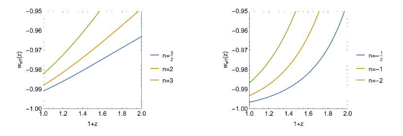
Figure 1: Qualitative evolution of the effective equation of state parameter $w_{eff}\left(z\right)$ as it is given by the numerical simulations of the dynamical system (75), (76) where $z$ is the redshift, $1+z=a^{-1}$. Plots are for initial conditions We have assumed the initial conditions $t_{0}$ is the present time, $a\left(t_{0}\right)=1$, $\phi\left(t_{0}\right)=1\,$. Left Fig. is for $I_{1}=0.01$, $\sqrt{-6V_{0}}=0.2$, while Right Fig. is for $I_{1}=-0.01$ and $\sqrt{-6V_{0}}=0.2$. The lines are for different values of parameter $n$ as they are given in the legends.

V.3 Connection $\Gamma^{C}$

For the field equations of the third connection $\Gamma^{C}$, and from the symmetry vector $Z_{3}$ we determine the similarity solution

$$a\left(t\right) = a_{0}\left(t-t_{0}\right)^{p_{1}},$$ (80)

$$\phi\left(t\right) = \phi_{0}\left(t-t_{0}\right)^{p_{2}},$$ (81)

$$\Psi\left(t\right) = \Psi_{0}\left(t-t_{0}\right)^{p_{3}},$$ (82)

where

$$p_{1} = \frac{3n-1}{5\left(n-1\right)},~$$ (83)

$$p_{2} = -\frac{2}{n-1},~$$ (84)

$$p_{3} = \frac{4\left(n-2\right)}{5\left(n-1\right)},$$ (85)

with constraints $\rho_{m0}=0$ and

$$V_{0} = \frac{12}{25}\phi_{0}^{1-n}\left(3n^{2}+8n-3\right),$$ (86)

$$\Psi_{0} = -\frac{25}{4a_{0}^{2}}\frac{\left(n-1\right)^{2}}{\left(3n^{3}-4n^{2}-5n+2\right)}.$$ (87)

This is a new exact cosmological solution that has not been reported so far.

V.4 Connection $\Gamma^{D}$

Finally, for the case with nonzero spatially curvature and connection $\Gamma^{D}$, we derive the similarity solution

$$a\left(t\right) = a_{0}\left(t-t_{0}\right)~,$$ (88)

$$\phi\left(t\right) = \phi_{0}\left(t-t_{0}\right)^{-1},$$ (89)

$$\Psi\left(t\right) = \Psi_{0}\ln\left(t-t_{0}\right),$$ (90)

in which $\rho_{m0}=0$ and

$$\Psi_{0} = -\frac{1}{3a_{0}^{2}},$$ (91)

$$V_{0} = \frac{4}{\phi_{0}}\left(3-\frac{k}{a_{0}^{2}}\right).$$ (92)

These results are in agreement with the scaling solutions determined in ndim1 . It is interesting to mention that the existence of the scaling solutions is related with the appearance of the Noether symmetry vectors.

VI Conclusion

The Noether symmetry analysis was applied to the field equations of symmetric teleparallel $f(Q)-$cosmology within an FLRW geometry. These field equations exhibit the property of admitting a minisuperspace description. In fact, there are four distinct families of connections for the FLRW geometry within symmetric teleparallel theory, each of which leads to a different minisuperspace Lagrangian.

By applying Noether’s theorem, we constrained the free functions and parameters of the four gravitational Lagrangian functions. The Noether symmetry condition led to the conclusion that the only function $f(Q)$ for which the field equations possess point symmetries is the power-law model. This result implies that, for any arbitrary $f(Q)-$theory, when the power-law components dominate, the gravitational field equations admit Noetherian conservation laws. These conservation laws can then be used to determine exact and analytic solutions.

This analysis opens new directions for exploring the integrability properties within the symmetric teleparallel theory of gravity, offering a promising framework for further investigation into conserved quantities and the exact solutions of $f(Q)$-gravity.

- (1) J.M. Nester and H.-J. Yo, Symmetric teleparallel general relativity, Chin. J. Phys. 37, 113 (1998)
- (2) J. B. Jimenez, L. Heisenberg and T. Koivisto, Phys. Rev. D 98, 044048 (2018)
- (3) J. B. Jimenez, L. Heisenberg, T. Sebastian Koivisto and S. Pekar, Phys. Rev. D 101, 103507 (2020)
- (4) S.A. Narawade, S.H. Shekh, B. Mishaa, W. Khyllep, J. Dutta, Eur. Phys. J. C 84, 773 (2024)
- (5) W. Khyllep, A. Paliathanasis and J. Dutta, Phys. Rev. D 103, 103521 (2021)
- (6) L. Järv, M. Rünkla, M. Saal and O. Vilson, Phys. Rev. D 97, 124025 (2018)
- (7) V. Gakis, M. Krššák, J.L. Said and E.N. Saridakis, Phys. Rev. D 101, 064024 (2020)
- (8) N. Dimakis, A. Giacomini, A. Yu Kamenshchik, G. Leon and A. Paliathanasis, Phys. Dark Univ. 44, 101436 (2024)
- (9) S.A. Narawade, M. Koussour and B. Mishra, Annalen Phys. 535, 2300161 (2023)
- (10) A. Paliathanasis, Phys. Dark Univ. 43, 101388 (2024)
- (11) A. De, T.-H. Loo and E.N. Saridakis, JCAP 03, 050 (2024)
- (12) S. Nojiri and S.D. Odintsov, Fortschritte der Physik - Progress of Physics 72, 2400113 (2024)
- (13) S.A. Narawade, S.P. Singh and B. Mishra, Phys. Dark Univ. 42, 101282 (2023)
- (14) A. Lymberis, JCAP 11, 018 (2022)
- (15) N. Dimakis, A. Paliathanasis and T. Christodoulakis, Class. Quantum Grav. 38, 225003 (2021)
- (16) J. Ferreira, T. Barreiro, J.P. Mimoso and N.J. Nunes, Phys. Rev. D 108, 063521 (2023)
- (17) F.K. Anagnostopoulos, S. Basilakos and E.N. Saridakis, Phys. Lett. B 822, 136634 (2021)
- (18) A. Samaddar, S.S. Singh, Md K. Alam, Grav. Cosmol. 30, 462 (2024)
- (19) V.C. Dubey, U.K. Sharma, S. Ray and A. Sanyal, Phys. Dark Univ. 47, 101736 (2025)
- (20) S. Mandal, A. Parida and P.K. Sahoo, Universe 8, 240 (2022)
- (21) Y. Carloni and O. Luongo, arXiv:2410.10935 (2024)
- (22) S. Bahamonte, J.G. Valcarcel, L. Jarv and J. Lember, JCAP 08, 082 (2022)
- (23) N. Dimakis, P.A. Terzis, A. Paliathanasis and T. Christodoulakis, JHEAp 45, 273 (2025)
- (24) D.J. Gogoi, A. Ovgun and M. Koussour, Eur. Phys. J. C 83, 700 (2023)
- (25) S.K. Maurya, A. Errehymy, Ksh.N. Singh, O. Donmez, K.S. Nisar and M. Mahmoud, Phys. Dark Univ. 46, 101619 (2024)
- (26) W. Wang, H. Chen and T. Katsuragawa, Phys. Rev. D 105, 024060 (2022)
- (27) L. Heisenberg, Phys. Reports 1066, 1 (2024)
- (28) T.P. Sotiriou and V. Faraoni, Rev. Mod. Phys. 82, 451 (2010)
- (29) A. De Felice and S. Tsujikawa, Living Rev. Rel. 13, 3 (2010)
- (30) S. Nojiri, S.D. Odintsov and D. Saez-Gomez, Phys. Lett. B 681, 74 (2009)
- (31) R. Ferraro and F. Fiorini, Phys. Rev. D 75, 084031 (2007)
- (32) R. Ferraro and F. Fiorini, Phys. Lett. B 702, 75 (2011)
- (33) T. Sotiriou and V. Faraoni, Rev. Mod. Phys. 82, 451 (2010)
- (34) S. Nojiri and S.D. Odintsov, Int. J. Geom.Meth. Mod. Phys. 4, 115 (2007)
- (35) S. Bahamonde, K. F. Dialektopoulos, C. Escamilla-Rivera, G. Farrugia, V. Gakis, M. Hendry, M. Hohmann, J. Levi Said, J. Mifsud and E. Di Valentino, Rept. Prog. Phys. 86, 026901 (2023)
- (36) A. Paliathanasis, N. Dimakis and T. Christodoulakis, Phys. Dark Univ. 43, 101410 (2024)
- (37) A. Bonanno, G. Esposito, C. Rubano and P. Scudellaro, Class. Quantum Grav. 24, 1443 (2007)
- (38) R. de Ritis, G. Marmo, G. Platania, C. Rubano and P. Scudellaro, Phys. Rev. D 42, 1091 (1990)
- (39) S. Mondal, R. Bhaumik, S. Dutta and S. Chakraborty, Mod. Phys. Lett. A 36, 2150246 (2021)
- (40) N. Dimakis, T. Christodoulakis and P.A. Terzis, J. Geom. Phys. 77, 97 (2014)
- (41) E. Massaeli, M. Motaharfar and H.R. Sepangi, EPJC 77, 124 (2017)
- (42) L. Anguelova, E.M. Babalic, C.I. Lazariou, JHEP 04, 148 (2019)
- (43) Y. Kucukakca and A.R. Akbarieh, EPJC 80, 1019 (2020)
- (44) S. Hembrom. R. Bhaumik, S. Dutta and S. Chakraborty, EPJC 84, 1054 (2024)
- (45) S. Capozziello, K.F. Dialektopoulos and S.V. Sushkov, EPJC 78, 447 (2018)
- (46) K.F. Dialektopoulos, J.L. Said and Z. Oikonomopoulou, EPJC 82, 259 (2022)
- (47) S. Basilakos, M. Tsamparlis and A. Paliathanasis, Phys. Rev. D 83, 103512 (2011)
- (48) M. Tsamparlis and A. Paliathanasis, Symmetry 10, 233 (2018)
- (49) K. F. Dialektopoulos and S. Capozziello, Int. J. Geom. Meth. Mod. Phys. 15, 1840007 (2018)
- (50) K.F. Dialektopoulos, T.S. Koivisto and S. Capozziello, EPJC 79, 606 (2019)
- (51) D. A. Gomes, J. Beltrán Jiménez, A. J. Cano and T. S. Koivisto, Phys. Rev. Lett. 132 (2024) no.14, 141401
- (52) M.J. Guzman, L. Jarv and L. Pati, Phys. Rev. D 110, 124013 (2024)
- (53) F. D’ Ambrosio, L. Heisenberg and S. Kuhn, Class. Quantum Grav. 39 025013 (2022)
- (54) N. Dimakis, A. Paliathanasis, M. Roumeliotis and T. Christodoulakis, Phys. Rev. D 106, 043509 (2022)
- (55) D. Zhao, Eur. Phys. J. C 82, 303 (2022)
- (56) G.W. Bluman and S. Kumei, Symmetries and Differential Equations, Springer: New York, (1989).
- (57) E. Noether, Invariante Variationsprobleme, Koniglich Gesellschaft der Wissenschaften Gottingen Nachrichten Mathematik-physik Klasse 2, 235 (1918)
- (58) Y. Kosmann-Schwarzbach and B.E. Schwarzbach, The Noether Theorems: Invariance and Conservation Laws in the Twentieth Century, Springer New York, New York (2011)
- (59) L. V. Ovsiannikov, Group analysis of differential equations, Academic Press, New York (1982)
- (60) A. Paliathanasis and M. Tsamparlis, J. Geom. Phys. 107, 45 (2016)
- (61) A. Paliathanasis, Phys. Dark Univ. 41, 101255 (2023)
- (62) A. Paliathanasis, Gen. Rel. Grav. 55, 130 (2023)
- (63) N. Dimakis, M. Roumeliotis, A. Paliathanasis, P.S. Apostolopoulos and T. Christodoulakis, Phys. Rev. D 106, 123516 (2022)