Generalized Simple Graphical Rules for Assessing Selection Bias

Abstract

Selection bias is a major obstacle toward valid causal inference in epidemiology. Over the past decade, several simple graphical rules based on causal diagrams have been proposed as the sufficient identification conditions for addressing selection bias and recovering causal effects. However, these simple graphical rules are usually coupled with specific identification strategies and estimators. In this article, we show two important cases of selection bias that cannot be addressed by these simple rules and their estimators: one case where selection is a descendant of a collider of the treatment and the outcome, and the other case where selection is affected by the mediator. To address selection bias in these two cases, we construct identification formulas by the g-computation and the inverse probability weighting (IPW) methods based on single-world intervention graphs (SWIGs). They are generalized to recover the average treatment effect by adjusting for post-treatment upstream causes of selection. We propose two IPW estimators and their variance estimators to recover the average treatment effect in the presence of selection bias in these two cases. We conduct simulation studies to verify the performance of the estimators when the traditional crude selected-sample analysis returns erroneous contradictory conclusions to the truth.
Keywords: selection bias, causal inference, causal diagrams, SWIG, inverse probability weighting, epidemiologic research

1 Introduction

Selection bias is one of the fundamental obstacles to causal inference. The concept of selection bias encompasses various forms stemming from different mechanisms for individuals being selected into the study or analysis [1]. The complexity of these selection mechanisms poses difficulty in a structural definition of selection bias, which has been continually evolving over the past two decades [2, 3, 4, 5]. Recently, a refined definition of selection bias that unifies different types of selection bias was proposed [3] by considering the true causal effect in the population prior to the selection process as the reference. This definition can be decomposed into two types: type 1 selection bias due to restricting to at least one level of a collider or its descendant, and type 2 selection bias due to restricting to at least one level of an effect measure modifier.[3]

With a clearer understanding of selection bias in place, recent methodological developments have also been dedicated to recovering causal effects in the presence of selection bias. Specifically, based on the fundamentals of causal diagrams, including directed acyclic graphs (DAGs) and single-world intervention graphs (SWIGs), simple graphical rules were proposed to account for selection bias, alone or possibly combined with other issues (e.g., confounding bias or missing data) [6, 7, 8, 9].

However, there are still important cases of selection bias that cannot be addressed by these existing graphical rules. For example, in the graphical rules proposed by Mathur and Shpitser, one premise is that post-treatment variables cannot be conditioned on in their selected-sample analysis estimator [8]. In addition, they focus on the conditional average treatment effect (CATE) rather than the average treatment effect (ATE, which is arguably more widely used). Some other existing graphical rules do not prohibit adjustments for post-treatment variables, but they are rather stringent to avoid confounding bias [10, 7, 6].

In some cases, the covariate information available to address selection bias may only include post-treatment variables [11]. In these cases, the identification of ATE may still be possible despite the rejection by the existing graphical rules. This highlights the importance of applying fundamental graphical rules to search for identification strategies. For example, approaches such as inverse probability weighting (IPW) methods and g-computation are powerful tools for recovering treatment effects if external information beyond the selected sample is available [1, 7, 11].

In this article, we discuss two important cases of selection bias unaddressed by existing graphical rules. The first one represents the selection bias where a descendant of a collider of the exposure and the outcome is being conditioned on. The other is an example where sample selection is affected by the mediator. We prove that the average treatment effect (ATE) in both cases can be recovered by the g-computation or IPW methods if the external information on the covariates is available in the general population. The conditions for proving these identification strategies are provided and can also be used for addressing selection bias in similar cases. We propose two specific IPW estimators and their variance estimators for the ATE. We conduct simulation studies to verify the statistical properties of the proposed IPW estimators. In our hypothetical simulation settings, we show that the conventional crude complete-case analysis using the selected sample yields conclusions contradictory to the truth and can mislead decision-making.

2 Two cases of selection bias unaddressed by simple graphical rules

To detect and control for selection bias, researchers usually consider some simple graphical rules along with a specific class of identification formulas, and then define ‘identifiability’ (or ‘recoverability’) in a narrow sense of whether the treatment effect of interest can be identified by that class of formulas [10, 7, 6, 8]. Simple graphical rules are usually sufficient conditions for verifying that the treatment effect can be identified (or recovered) by a particular class of identification formulas. If these conditions are violated, it does not rule out the possibility that the effect of interest can still be identified by other formulas. In this section, we show two important cases of selection bias that cannot be addressed by the previously proposed graphical rules. The identification of treatment effects for similar causal structures by modified formulas will be discussed in later sections.

2.1 Setting

Consider $n$ individuals (hereafter called “unit”) in a randomized clinical trial whose outcomes are observed only among selected units. The selection is directly affected by a post-treatment variable observable among all units. Specifically, let $A_{i}$ be the binary treatment for unit $i$, $Y_{i}$ be the binary outcome, and $S_{i}$ be the selection. There are no other variables as confounders of $A_{i}$ and $Y_{i}$. We define the direct upstream cause of the selection to be $L_{i}$, which can be either a common effect of the treatment and the outcome (Case 1 in Fig. 1), or a mediator of the treatment on the outcome (Case 2 in Fig. 1). When a unit is selected, i.e. $S_{i}=1$, we observe all variables $(A_{i},Y_{i},L_{i})$. When a unit is not selected, i.e. $S_{i}=0$, we observe its direct upstream cause $L_{i}$ along with the knowledge of $A_{i}$ or the rule of treatment assignment $p(A_{i}=1)$ while the outcome $Y_{i}$ remains unobserved. We denote potential responses to a particular treatment $A_{i}=a_{i}$ by $(Y_{i}(a_{i}),L_{i}(a_{i}),S_{i}(a_{i}))$, which are affected by the treatment in both cases. Under the consistency assumption, $(Y_{i}(a_{i}),L_{i}(a_{i}),S_{i}(a_{i}))$ = $(Y_{i},L_{i},S_{i})$.

Both Case 1 and Case 2 are important as they represent scenarios that may occur in real-world settings. For example, consider Case 1, where the study is a randomized trial of a prophylactic medication for malaria among susceptibles. The treatment $A$ is a binary variable indicating assignment to the medication or not. The outcome of interest $Y$ is the incidence of malaria or not. The incidence of fever or not, $L$, directly affects the receipt of the blood test for malaria or not, $S$, for the outcome to be detected. It was suggested that the selection bias in this exact causal graph cannot be addressed to recover the ATE by the selection-backdoor criteria [6].

In Case 2, the study is a randomized trial of a vaccine for an infectious disease with multiple endpoints. The treatment $A$ indicates assignment to the vaccine or not. The outcome $Y$ is the symptom of having a headache or not. The outcome is mediated by the incidence of infection, $L$, which also affects whether a unit reports the outcome status, $S$.

Assume that our goal is to recover the average treatment effect (ATE) in the general population prior to the selection process:

$$\delta_{\text{ATE}}=\mathbb{E}[Y(1)-Y(0)].$$

Figure 1: Causal directed acyclic graphs (DAGs) and single-world intervention graphs (SWIGs) for Case 1 and Case 2 of sample selection directly affected by a post-treatment variable $L$. When a unit is selected into the sample (i.e. $S_{i}=1$), we observe all variables $(A_{i},Y_{i},L_{i})$. When a unit is not selected (i.e. $S_{i}=0$), external information on $L_{i}$ among unselected units, along with the knowledge of $A_{i}$ or the rule of treatment assignment $p(A_{i}=1)$, might still be available, but the outcome $Y_{i}$ is unobserved. In Case 1, the direct upstream cause of selection, $L$, is the common effect (i.e., collider) of both the treatment $A$ and the outcome $Y$. In Case 2, the direct upstream cause of selection, $L$, is the mediator of the treatment $A$ on the outcome $Y$.

2.2 The failure by existing simple graphical rules

We focus on three existing simple graphical rules (i.e., the selection-backdoor criterion [6], the generalized adjustment criterion [7], and Mathur and Shpitser’s graphical rules [8]) proposed over the past decade. In Appendix A, we show that the two cases as discussed above violate these existing simple graphical rules, and the identification by their corresponding formulas is not guaranteed.

3 Identification by the fundamentals of graphical rules

In this section, we first introduce a g-computation formula that can be used to recover the ATE by conditioning on post-treatment variables [11]. Then we propose the inverse probability weighting (IPW) method to recover the ATE and address selection bias in the two cases discussed. The identification results by the two proposed methods are generalized under specific graphical rules to allow (i) observed confounders for the relationships between the treatment and post-treatment variables, (ii) unobserved confounders for the relationships between post-treatment variables and the outcome, and (iii) selection that is directly affected by the treatment.

3.1 G-computation formulas

In Breskin et al.[11], a special-case g-formula conditioning on a post-treatment variable $Z$ was derived for identifying the ATE in a practical example of randomized controlled trials, demonstrating the utility of SWIGs. We extend their results by allowing the existence of confounders in an observational setting.

Specifically, we propose the following theorem.

Theorem 1 (Identification of the ATE by the g-formula under selection bias).

Given a SWIG $\mathcal{G}(a)$ containing the random treatment component $A$, the fixed treatment component $a$, the post-treatment variables $Z(a)$, the selection variable $S(a)$, the outcome variable $Y(a)$, the observed pre-treatment variables $X$, and the unobserved pre-treatment variables $U$, the ATE is identified by

$$\begin{split}\delta_{\text{ATE},g}=\sum_{x}(\sum_{z}&\mathbb{E}[Y|A=1,Z=z,S=1,X=x]p(Z=z|A=1,X=x)-\\ &\mathbb{E}[Y|A=0,Z=z,S=1,X=x]p(Z=z|A=0,X=x))p(X=x),\end{split}$$ (1)

i.e. $\delta_{\text{ATE}}=\delta_{\text{ATE},g}$, if the following conditions hold:

$$\begin{split}&(C1)\quad Y(a)\perp\!\!\!\!\perp S(a)|Z(a),X\\ &(C2)\quad Y(a)\perp\!\!\!\!\perp A|Z(a),S(a),X\\ &(C3)\quad Z(a)\perp\!\!\!\!\perp A|X.\end{split}$$ (2)

Intuitively, the first condition assumes that all paths between $Y(a)$ and $S(a)$ are blocked by $Z(a)$ and $X$. This motivates the adjustment of some post-treatment variables $Z(a)$ if it helps separate the outcome from the selection. The next two conditions assume that the effect of the treatment on both $Y(a)$ and $Z(a)$ are unconfounded by conditioning on different sets of variables.

Therefore, despite being motivated by an ad-hoc estimator for a special case, the g-formula (1) will recover the ATE when some post-treatment variables can be conditioned on to address selection bias. The conditions can be viewed as derived graphical rules in this specific context. The example by Breskin et al. [11] is a special case of our theorem (where they denote the post-treatment variable by $W$ instead of $L$) by the following corollary.

Corollary 1 (Identification of the ATE by the g-formula given SWIG [11]).

The ATE is identified by

$$\begin{split}\delta_{\text{ATE},g}=\sum_{w}&\mathbb{E}[Y|A=1,W=w,S=1]p(W=w|A=1)-\\ &\mathbb{E}[Y|A=0,W=w,S=1]p(W=w|A=0),\end{split}$$

i.e. $\delta_{\text{ATE}}=\delta_{\text{ATE},g}$, for the SWIG in Breskin et al.[11].

Taking $Z=L$, our Case 2 can be considered as a modification of the graph in Breskin et al. [11] where the derivation of the formula still applies. Moreover, it is straightforward to verify that the conditions (2) are satisfied in both of our cases by the SWIGs in Fig. 1. We have the following corollary as examples.

Corollary 2 (Identification of the ATE by the g-formula given Fig. 1).

The ATE is identified by

$$\begin{split}\delta_{\text{ATE},g}=\sum_{l}&\mathbb{E}[Y|A=1,L=l,S=1]p(L=l|A=1)-\\ &\mathbb{E}[Y|A=0,L=l,S=1]p(L=l|A=0),\end{split}$$

i.e. $\delta_{\text{ATE}}=\delta_{\text{ATE},g}$, for the two SWIGs in Fig. 1.

The theorem implies that the ATE can still be recovered if we extend the two cases in Fig. 1 to allow observed confounders $X=(X_{1},X_{2},X_{3})$ for $A$ and $(Y,L,S)$ (i.e., treatment-post-treatment-variable confounders) in the full population, respectively, and unobserved confounders $U$ for $L$ and $Y$ (i.e., collider-outcome confounders, or mediator-outcome confounders) as in Fig. 2.

Corollary 3 (Identification of the ATE by the g-formula given Fig. 2).

The ATE is identified by

$$\begin{split}\delta_{\text{ATE},g}=\sum_{x}(\sum_{l}&\mathbb{E}[Y|A=1,L=l,S=1,X=x]p(L=l|A=1,X=x)-\\ &\mathbb{E}[Y|A=0,L=l,S=1,X=x]p(L=l|A=0,X=x))p(X=x),\end{split}$$

i.e. $\delta_{\text{ATE}}=\delta_{\text{ATE},g}$, for the two SWIGs in Fig. 2.

Note that the ATE is identified even when $X=(X_{1},X_{2})$. In other words, the treatment-selection confounders, $X_{3}$, are not required to be observed for recovering the ATE for the two cases in Fig. 2 by this g-formula. The intuition is that, if there exists some post-treatment variable $L(a)$ as the direct cause of selection that helps separate $Y(a)$ from $S(a)$, the selection $S(a)$ becomes a collider on the backdoor paths from the treatment $A$ to $L(a)$ and $Y(a)$ that go through $X_{3}$. Therefore, these backdoor paths ($A\leftarrow X_{3}\rightarrow S(a)\leftarrow L(a)$ and $A\leftarrow X_{3}\rightarrow S(a)\leftarrow L(a)\leftarrow Y(a)$) are blocked without the need to adjust for $X_{3}$ to correct confounding bias.

Proofs of Theorem 1 and its corollaries are given in Appendix B.

For estimation and inference by the g-formulas, plug-in estimators can be applied and the variances can be derived using the delta method or bootstrap [14].

Figure 2: Causal directed acyclic graphs (DAGs) and single-world intervention graphs (SWIGs) for Case 1 and Case 2 of sample selection directly affected by a post-treatment variable $L$ with observed covariates $X=(X_{1},X_{2},X_{3})$ and unobserved covariates $U$. When a unit is selected (i.e. $S_{i}=1$), we observe all variables $(X_{i},A_{i},Y_{i},L_{i})$. When a unit is not selected (i.e. $S_{i}=0$), external information on $(X_{i},A_{i},L_{i})$ among unselected units might still be available. Case 1: The direct upstream cause of selection, $L$, is the common effect (i.e., collider) of the treatment $A$ and the outcome $Y$. Case 2: The direct upstream cause of selection, $L$, is the mediator on the causal pathway from treatment $A$ to the outcome $Y$.

3.2 Inverse probability weighting

Inverse probability weighting (IPW) methods intuitively create a pseudo-population where the distributions of covariates are balanced across treatment groups to fix the endogeneity of treatment and recover its effects [15, 16]. They have also been recognized and applied for the generalizability and transportability of study results to a target population of interest that is different from the study sample [17, 18, 19, 20, 21, 22].

In the context of selection bias, if external information on the distribution of the post-treatment variable $L$, is available, it is also possible to reweight the distributions of post-treatment variables such that they are not skewed by sample selection among the pseudo-population, thereby addressing selection bias. We propose a theorem to formalize the idea.

Theorem 2 (Identification of the ATE by the IPW method under selection bias).

Given a SWIG $\mathcal{G}(a)$ containing the random treatment component $A$, the fixed treatment component $a$, the post-treatment variables $Z(a)$, the selection variable $S(a)$, the outcome variable $Y(a)$, the observed pre-treatment variables $X$, and the unobserved pre-treatment variables $U$, the ATE is identified by

$$\begin{split}\delta_{\text{ATE},\text{IPW}}=\mathbb{E}[\frac{ASY}{p(S=1|Z,X,A)p(A=1|X)}]-\mathbb{E}[\frac{(1-A)SY}{p(S=1|Z,X,A)p(A=0|X)}],\end{split}$$ (3)

i.e. $\delta_{\text{ATE}}=\delta_{\text{ATE},\text{IPW}}$, if the following conditions hold:

$$\begin{split}&(C1)\quad Y(a)\perp\!\!\!\!\perp S(a)|Z(a),X\\ &(C2)\quad(Y(a),S(a))\perp\!\!\!\!\perp A|Z(a),X\\ &(C3)\quad Z(a)\perp\!\!\!\!\perp A|X\\ \end{split}$$ (4)

The first condition assumes that all paths between $Y(a)$ and $S(a)$ are blocked by $Z(a)$ and $X$. The next two conditions assume that the treatment and the potential responses of post-treatment variables (including the outcome, covariates, and selection) can be sequentially separated. The second condition for the IPW method (4) is slightly different from that for the g-formula (2). The requirement by the IPW method that $S(a)$ should be conditionally separated from $A$ is due to the inclusion of the inverse probability weighting model for the selection to recover the ATE.

The ATE can be recovered through the IPW method in all causal graphs in Breskin et al.[11], Fig. 1, and Fig. 2. They are special cases of Theorem 2 by the following corollaries.

Corollary 4 (Identification of the ATE by the IPW method given SWIG [11]).

The ATE is identified by

$$\begin{split}\delta_{\text{ATE},\text{IPW}}=\mathbb{E}[\frac{ASY}{p(S=1|W)p(A=1)}]-\mathbb{E}[\frac{(1-A)SY}{p(S=1|W)p(A=0)}],\end{split}$$

i.e. $\delta_{\text{ATE}}=\delta_{\text{ATE},\text{IPW}}$, for the SWIG in Breskin et al.[11].

Corollary 5 (Identification of the ATE by the IPW method given Fig. 1).

The ATE is identified by

$$\begin{split}\delta_{\text{ATE},\text{IPW}}=\mathbb{E}[\frac{ASY}{p(S=1|L)p(A=1)}]-\mathbb{E}[\frac{(1-A)SY}{p(S=1|L)p(A=0)}],\end{split}$$

i.e. $\delta_{\text{ATE}}=\delta_{\text{ATE},\text{IPW}}$, for the two SWIGs in Fig. 1.

Corollary 6 (Identification of the ATE by the IPW method given Fig. 2).

The ATE is identified by

$$\begin{split}\delta_{\text{ATE},\text{IPW}}=\mathbb{E}[\frac{ASY}{p(S=1|L,X,A)p(A=1|X)}]-\mathbb{E}[\frac{(1-A)SY}{p(S=1|L,X,A)p(A=0|X)}],\end{split}$$

i.e. $\delta_{\text{ATE}}=\delta_{\text{ATE},\text{IPW}}$, for the two SWIGs in Fig. 2.

The treatment-selection confounders $X_{3}$ cannot be omitted by the IPW method for recovering the ATE because the model for the selection deems it necessary to collect and adjust for these variables for correct causal model specification. This is different from the requirements by the g-formula for the same graph.

Proofs of Theorem 2 and its corollaries are given in Appendix B.

4 Estimation and inference by IPW estimators

Based on the identification result in Theorem 2, an unbiased estimator of the ATE is the Hovitz-Thompson (HT) estimator. We also propose an alternative IPW estimator, the Hájek estimator, which is a biased estimator of the ATE but reduces variance compared to the HT estimator [23]. We propose closed-form sandwich estimators of their variances to enable statistical inference of the ATE [24]. We use the two cases in Fig. 1 as demonstrative examples by Corollary 5. We outline the steps of estimation and inference in Appendix C.

5 Simulation

We conduct simulation studies to verify the performance of our IPW estimators in both cases of Fig. 1. The null hypothesis of the treatment effect is set to be true in the first case, but not in the second case. For each case, we generate datasets with varying sample sizes of $n=100,n=1000,n=10000$. The two IPW estimators are compared to the crude selected-sample analysis which only includes the observed treatment $A$ in the simple linear regression of the observed outcome $Y$. In each setting, we simulate $K=10000$ datasets and fit the models. We show that the crude analysis yields biased and misleading conclusions but our IPW methods accurately recover the true effect.

In Case 1, consider a randomized trial of a prophylactic medication for malaria among susceptible individuals. The treatment ($A$) is a binary variable indicating whether an individual is randomly assigned to the medication or not. The outcome of interest ($Y$) indicates the incidence of malaria or not, which is detected by a blood test. The ground truth is that the medication has a null effect on the outcome. However, both the medication and malaria increase the risk of fever. The incidence of fever or not ($L$) will be reported by these individuals. It affects participants’ willingness to receive the blood test for malaria or not ($S$). Those who have a fever are more likely to receive the blood test, while those who do not have a fever feel less motivated to be tested. Specifically, We simulate observed data from the following distributions:

$$\begin{split}&A_{i}\sim Bernoulli(0.5)\\ &Y_{i}|A_{i}=a_{i}\sim Bernoulli(0.4)\\ &L_{i}|A_{i}=a_{i},Y_{i}=y_{i}\sim Bernoulli(0.1+0.3a_{i}+0.5y_{i})\\ &S_{i}|L_{i}=l_{i}\sim Bernoulli(0.1+0.8l_{i}).\end{split}$$

The true ATE of the treatment is $0$, meaning that the medication on average has a zero impact on reducing the risk of malaria.

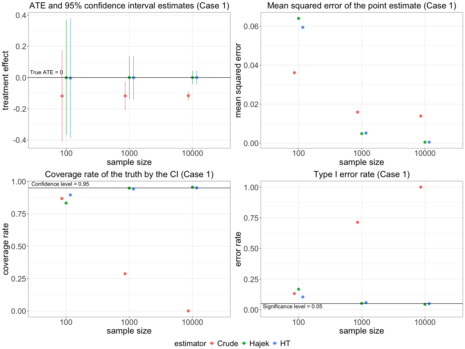
Figure 3: Case 1: simulation results of average point estimates of ATE, mean squared error, confidence intervals, coverage rates of the true ATE by the 95% confidence interval, and the type I error rate by the crude selected-sample analysis using the selected sample and the two proposed IPW estimators under different sample sizes. The true ATE is 0 for Case 1.

The crude selected-sample analysis (i.e., crude complete-case analysis) in Case 1 (red colored in Fig. 3) erroneously concludes a beneficial effect of the medication on reducing the risk of malaria. The $95\%$ confidence interval only contains the truth when the sample size is small due to substantial uncertainty. The coverage rates of the truth, zero effect, by its $95\%$ confidence interval drops to zero as the sample size increases. In this null effect case, it implies that the rejection rate rises to $100\%$ as the sample size increases. The intuition is that, with a low probability of measuring the outcome among those who do not have a fever, individuals who are not assigned to the medication and do not have malaria are unlikely to be selected. Without information from these healthy individuals, the effect of the medication is overestimated, leading to selection bias. As a result, the crude selected-sample analysis yields a misleading result by exaggerating the impact of the medication.

The results by the IPW estimators are summarized for Case 1 in Fig. 3 (green and blue colored). Point estimates by both methods are correctly centered around zero. The mean squared error quickly drops and approaches zero. The coverage rates of the truth by the $95\%$ confidence intervals converge towards $95\%$ as the sample size increases. Equivalently, the type I error rate of rejecting the null hypothesis approaches $5\%$. Both methods are expected to fail to reject the null hypothesis at the intended size. The Hájek estimator has slightly smaller variances and narrower confidence intervals than the HT estimator.

In Case 2, consider a randomized trial of some vaccine for an infectious disease that assigns half of the individuals to the treatment group. One of the endpoints in this trial is the risk of having a headache within a certain period. The treatment ($A$) is random assignment to the vaccine or the placebo group. Its effect on the outcome of having a headache or not ($Y$), can be directly through its side effects by increasing the risk. It can also be indirectly, mediated by the risk of being infected. The incidence of infection ($L$) affects the chance that they report whether they had a headache ($S$) during that period. Infected individuals are more likely to have a hospital encounter and report their symptoms in terms of headache, but those uninfected are less likely to report having headache symptoms or not unless through follow-up contacts. The data-generating process is

$$\begin{split}&A_{i}\sim Bernoulli(0.5)\\ &L_{i}|A_{i}=a_{i}\sim Bernoulli(0.7-0.5a_{i})\\ &Y_{i}|A_{i}=a_{i},L_{i}=l_{i}\sim Bernoulli(0.1+0.1a_{i}+0.5l_{i})\\ &S_{i}|L_{i}=l_{i}\sim Bernoulli(0.1+0.8l_{i}).\end{split}$$

By Corollary 2, the true ATE is $-0.15$, indicating that the vaccination on average reduces the risk of headache by $15\%$.

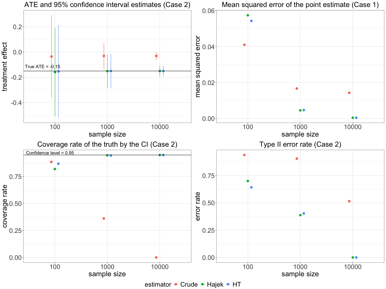
Figure 4: Case 2: simulation results of average point estimates of ATE, mean squared error, confidence intervals, coverage rates of the true ATE by the 95% confidence interval, and the type II error rate by the crude complete-case analysis using the selected sample and the two proposed IPW estimators under different sample sizes. The true ATE is -0.15 for Case 2.

The crude selected-sample analysis of Case 2 (red colored in Fig. 4) exhibits biased estimates of the ATE as small as $-0.03$. The $95\%$ confidence intervals contain zero across all three settings. Similar to Case 1, the coverage rate of the true ATE also drops to zero when the sample size increases. The rejection rate is lower than $10\%$ when the sample size is $1000$ or smaller, indicating a type II error rate higher than $90\%$. When the sample size reaches $1000$, the type II error rate is still higher than $50\%$. The explanation is that the decreased chance of reporting whether an individual has a headache among those uninfected partly masks the beneficial indirect effect of the vaccine on reducing headaches through reducing their risk of infection. Therefore, the crude selected-sample analysis fails to reveal the actual beneficial impact of the vaccination on reducing the overall risk of headaches.

Tabel 4 shows the results of the IPW estimators for Case 2 (colored in green and blue). Both methods successfully recover the true ATE around $-0.15$ across all sample sizes. The mean squared error converges to zero. The coverage rates of the true ATE by the $95\%$ confidence interval increase to the intended level. The rejection rates increases to $100\%$ when the sample size is large enough. The power of the two methods with a sample size of $1000$ is greater than that of the crude selected-sample analysis with a sample size of $10000$ by over $10\%$.

6 Discussion

Our work assesses and extends the utility of existing graphical rules for addressing selection bias. Derived based on the fundamental principle of reading conditional independence using d-separation, existing simple graphical rules are inherently coupled with certain identification formulas and applicable to resolving selection bias for a specific subset of selection mechanisms. We show that, some important existing rules [6, 7, 8] can have stringent requirements on covariate adjustment to avoid confounding bias while correcting selection bias. For example, the adjustment for post-treatment variables is generally discouraged by these rules even if it helps separate the selection from the outcome. It is worth noting that while post-treatment variables should not be adjusted for in addressing confounding bias, these variables can indeed be accounted for when dealing with selection bias. We use two concrete examples using causal diagrams to demonstrate the limitations of existing rules and their identification strategies in addressing selection bias.

Specific to the two examples, we theoretically prove the identifiability of the ATE by the g-formula and the IPW method when relevant external information in the full population is available. The g-formula relies on adjusting for the post-treatment upstream cause of selection using a conditional distribution, while the IPW method seeks to balance the distributions of variables by modeling the probability of selection in the full population. The characteristics of these approaches are related to different sufficient conditions that we propose for recovering the ATE. They can be applied to complex observational settings with observed confounders for the relationships between the treatment and post-treatment variables, and unobserved confounders for the relationships between the upstream cause of selection and the outcome. For the IPW method, we also propose two estimators and their variance estimators for the statistical inference of the ATE. We outline the procedures and conducte simulation analysis to verify the performance of our estimators, which correct the serious bias by a complete-case analysis using the selected sample.

Beyond the two examples, our approach to correcting the selection bias validates and suggests possible directions for recovering the ATE when conventional approaches fail. First, researchers have shown that the g-formula and the IPW method are reliable alternatives to the oftentimes biased selected-sample analysis, for addressing selection bias and beyond [25, 14, 17, 18, 19, 11, 20, 21, 22]. Second, it is possible to adjust for post-treatment variables to recover the intended treatment effect without incurring overadjustment bias [26, 27, 28]. The adjustment is in a broader sense that its conditional distribution might be marginalized, or it might be included in a model for the selection, rather than a simple inclusion of it in the outcome regression.

In conclusion, selection bias will continue to be a key topic in epidemiological research. Recent advancements in conceptualizing and addressing selection bias, along with future developments, will bring us closer to a comprehensive understanding of this critical issue.

Acknowledgements

This section has been temporarily removed from the manuscript for peer review.

Appendix A Failure of identification by existing simple graphical rules

A.1 The selection-backdoor criterion

The backdoor criterion was proposed to address confounding bias based on DAGs [30]. It was extended to be the selection-backdoor criterion to assess whether conditioning on certain variables $Z$ simultaneously fixes selection bias and confounding bias [6]. The criterion conditions are as follows.

Definition 1 (The selection-backdoor criterion [31]).

Let a set $Z$ of variables be partitioned into $Z^{+}\cup Z^{-}$ such that $Z^{+}$ contains all nondescendants of $A$ and $Z^{-}$ the descendants of $A$. $Z$ is said to satisfy the selection backdoor criterion relative to an ordered pair of variables $(A,Y)$ and an ordered pair of sets $(M,T)$ in a graph $G_{s}$, where $M$ are variables collected under selection bias, $P(M|S=1)$, and $T$ are variables collected in the population-level, $P(T)$, if $Z^{+}$ and $Z^{-}$ satisfy the following conditions:

$$\begin{split}&\text{(i) $Z^{+}$ blocks all back door paths from $A$ to $Y$}\\ &\text{(ii) $A$ and $Z^{+}$ block all paths between $Z^{-}$ and $Y$, namely, $(Z^{-}\perp\!\!\!\!\perp Y|A,Z^{+})$}\\ &\text{(iii) $A$ and $Z$ block all paths between $S$ and $Y$, namely, $(Y\perp\!\!\!\!\perp S|A,Z)$}\\ &\text{(iv) $Z\cup\{A,Y\}\subseteq M$, and $Z\subseteq T$}.\end{split}$$

The first two conditions extend the backdoor criterion to control for confounding. The third and fourth conditions allow recoverability from selection bias. If the criterion holds, the identification formula for ATE is given by

$$\Delta_{\text{ATE},1}=\sum_{z}(\mathbb{E}[Y|A=1,Z=z,S=1]-\mathbb{E}[Y|A=0,Z=z,S=1])p(Z=z).$$ (5)

For each of the two cases in Fig. 1, we consider two estimators, conditioning on $L$ ($Z=L$), or not ($Z$ empty). For both cases, when we condition on $L$, condition (ii) in the selection-backdoor criterion does not hold. This condition requires that any path between the post-treatment variable $L$, if it is conditioned on, and the outcome $Y$ must be blocked by the treatment or other pre-treatment variables. In other words, there must not be any causal paths between the post-treatment variable that we condition on, and the outcome. Alternatively, when there is no conditioning on any variable $Z$, condition (iii) in the selection-backdoor criterion, which requires any path between the outcome $Y$ and the selection $S$ must be blocked by the conditioned variables, does not hold. To summarize, by selection-backdoor criterion, conditioning on $L$ violates the strong condition for ensuring no confounding bias, while not conditioning on $L$ fails to address selection bias. The ATE is unidentified by formula (5).

A.2 The Generalized Adjustment Criterion by Correa et al.

Following the selection-backdoor criterion based on DAGs, the Generalized Adjustment Criteria were proposed as sufficient and necessary conditions for the assertion of identification or not by certain formulas. Among them, Generalized Adjustment Criterion Type 3 (GACT3) provides the most general conditions for recovering the ATE by a flexible formula that allows the combination of external data and biased selected data [7].

Definition 2 (The Generalized Adjustment Criterion Type 3 (GACT3) [7]).

Given a causal diagram $G$ augmented with selection variable $S$, disjoint sets of variables $A$, $Y$, $Z$ and a set $Z^{T}\subseteq Z$; $(Z,Z^{T})$ is an admissible pair relative to $A$, $Y$ in $G$ if:

$$\begin{split}&\text{(a) No element in $Z$ is a descendant in $G_{\bar{A}}$ of any $W\notin A$ lying on a proper}\\ &\text{causal path from $A$ to $Y$}\\ &\text{(b) All non-causal paths in $G$ from $A$ to $Y$ are blocked by $Z$ and $S$}\\ &\text{(c) $Z^{T}$ d-separates $Y$ from $S$ in the proper backdoor graph, where the first}\\ &\text{edge of every proper causal path from $A$ to $Y$ is removed}.\end{split}$$

The first two conditions control confounding bias and the last condition controls selection bias. The identification formula is

$$\begin{split}\Delta_{\text{ATE},2}=\sum_{z}&(\mathbb{E}[Y|A=1,Z=z,S=1]-\mathbb{E}[Y|A=0,Z=z,S=1])\\ &p(Z\backslash Z^{T}=z\backslash z^{T}|Z^{T}=z^{T},S=1)p(Z^{T}=z^{T}),\end{split}$$ (6)

where $Z$ is the full set of variables being conditioned on, and $Z^{T}$ is a subset of $Z$ that requires external measurement. If we condition on $Z=L$, in either of both cases, condition (a) in GACT3 is violated. If the conditioning set is empty, Case 1 violates condition (b) and (c) while Case 2 violates condition (c). It proves that the ATE can not be identified by formula (6).

A.3 Simple graphical rules under SWIG by Mathur and Shpitser

Graphical rules based on SWIGs were also proposed for addressing selection bias [8]. It involves two sufficient conditions to analyze whether a conditional average treatment effect (CATE) can be identified by their formula.

Definition 3 (The graphical rules for assessing selection bias [8]).

Given a single-world intervention template $\mathcal{G}(a)$, the graphical rules are

$$\begin{split}&\text{(C1) }Y(a)\perp\!\!\!\!\perp A|S(a),Z\\ &\text{(C2) }Y(a)\perp\!\!\!\!\perp S(a)|Z.\end{split}$$

A premise of the two conditions in their framework is that the conditioning is on pre-treatment variables only. The first rule ensures no unadjusted confounding by conditioning on the selection and a set of adjusted covariates, and the second rule ensures no selection bias by conditioning on the same set of covariates. On its basis, a direct extension of their formula for the CATE to the ATE also follows formula (5). Despite changing the graphical rules, the ATE still fails to be identified in both cases when there is no conditioning, because the second condition that tries to separate between $S(a)$ and $Y(a)$ does not hold. Identification by conditioning on $L$ is not accommodated in these simple graphical rules because $L$ is a post-treatment variable. Therefore, the ATE is not identified by formula (5), again.

Appendix B Proof of theoretical results

B.1 Proof of Theorem 1

Proof of Theorem 1.

$$\begin{split}&\mathbb{E}[Y(a)]\\ =&\sum_{x}\mathbb{E}[Y(a)|X=x]p(X=x)\\ =&\sum_{x}\sum_{z}\mathbb{E}[Y(a)|Z(a)=z,X=x]p(Z(a)=z|X=x)p(X=x)\\ =&\sum_{x}\sum_{z}\mathbb{E}[Y(a)|Z(a)=z,S(a)=1,X=x]p(Z(a)=z|X=x)p(X=x)\\ =&\sum_{x}\sum_{z}\mathbb{E}[Y(a)|Z(a)=z,S(a)=1,X=x,A=a]p(Z(a)=z|X=x,A=a)p(X=x)\\ =&\sum_{x}\sum_{z}\mathbb{E}[Y|Z=z,S=1,X=x,A=a]p(Z=z|X=x,A=a)p(X=x),\end{split}$$

where the third equation is by (C1) in conditions (2), the fourth equation is by (C2) and (C3), and the last equation is by consistency. ∎

B.2 Proof of Corollary 1

Proof of Corollary 1.

Let $X$ be an empty set. The conditions (2) hold for the SWIG in Breskin et al.[11] where $Z=W$. By Theorem 1, the g-formula is reduced to

$$\begin{split}\delta_{\text{ATE},g}=\sum_{z}&\mathbb{E}[Y|A=1,Z=z,S=1]p(Z=z|A=1)-\\ &\mathbb{E}[Y|A=0,Z=z,S=1]p(Z=z|A=0),\end{split}$$

∎

B.3 Proof of Corollary 2

Proof of Corollary 2.

Let $X$ be an empty set and $Z=L$. The conditions (2) hold for the SWIGs in Fig. 1. By Theorem 1, the g-formula is reduced to

$$\begin{split}\delta_{\text{ATE},g}=\sum_{z}&\mathbb{E}[Y|A=1,Z=z,S=1]p(Z=z|A=1)-\\ &\mathbb{E}[Y|A=0,Z=z,S=1]p(Z=z|A=0),\end{split}$$

∎

B.4 Proof of Corollary 3

Proof of Corollary 3.

Let $Z=L$. The conditions (2) hold for the SWIGs in Fig. 2 taking $X=(X_{1},X_{2},X_{3})$ or $X=(X_{1},X_{2})$. By Theorem 1, the g-formula is

$$\begin{split}\delta_{\text{ATE},g}=\sum_{x}(\sum_{z}&\mathbb{E}[Y|A=1,Z=z,S=1,X=x]p(Z=z|A=1,X=x)-\\ &\mathbb{E}[Y|A=0,Z=z,S=1,X=x]p(Z=z|A=0,X=x))p(X=x),\end{split}$$

∎

B.5 Proof of Theorem 2

Proof of Theorem 2.

$$\begin{split}&\quad\ \mathbb{E}[\frac{1(A_{i}=a,S_{i}=1)Y_{i}}{p(S_{i}=1|Z_{i},X_{i},A_{i})p(A_{i}=a|X_{i})}]\\ &=\mathbb{E}[\frac{1(A_{i}=a,S_{i}(a)=1)Y_{i}(a)}{p(S_{i}(a)=1|Z_{i}(a),X_{i},A_{i}=a)p(A_{i}=a|X_{i})}]\\ &=\mathbb{E}[\mathbb{E}[\frac{1(A_{i}=a,S_{i}(a)=1)Y_{i}(a)}{p(S_{i}(a)=1|Z_{i}(a),X_{i},A_{i}=a)p(A_{i}=a|X_{i})}|Z_{i}(a),X_{i}]]\\ &=\mathbb{E}[\frac{\mathbb{E}[1(A_{i}=a,S_{i}(a)=1)Y_{i}(a)|Z_{i}(a),X_{i}]}{p(S_{i}(a)=1|Z_{i}(a),X_{i},A_{i}=a)p(A_{i}=a|X_{i})}]\\ &=\mathbb{E}[\frac{\mathbb{E}[1(A_{i}=a)|Z_{i}(a),X_{i}]\mathbb{E}[1(S_{i}(a)=1)Y_{i}(a)|Z_{i}(a),X_{i}]}{p(S_{i}(a)=1|Z_{i}(a),X_{i},A_{i}=a)p(A_{i}=a|X_{i})}]\\ &=\mathbb{E}[\frac{\mathbb{E}[1(A_{i}=a)|Z_{i}(a),X_{i}]\mathbb{E}[1(S_{i}(a)=1)|Z_{i}(a),X_{i}]\mathbb{E}[Y_{i}(a)|Z_{i}(a),X_{i}]}{p(S_{i}(a)=1|Z_{i}(a),X_{i},A_{i}=a)p(A_{i}=a|X_{i})}]\\ &=\mathbb{E}[\frac{\mathbb{E}[1(A_{i}=a)|X_{i}]\mathbb{E}[1(S_{i}(a)=1)|Z_{i}(a),X_{i},A_{i}=a]\mathbb{E}[Y_{i}(a)|Z_{i}(a),X_{i}]}{p(S_{i}(a)=1|Z_{i}(a),X_{i},A_{i}=a)p(A_{i}=a|X_{i})}]\\ &=\mathbb{E}[\mathbb{E}[Y_{i}(a)|Z_{i}(a),X_{i}]]\\ &=\mathbb{E}[Y_{i}(a)].\end{split}$$

The first equation is by consistency. The fourth equation is by (C2) in conditions (4). The fifth equation is by (C1). The sixth equation is by (C2) and (C3). ∎

B.6 Proof of Corollary 4

Proof of Corollary 4.

Let $X$ be an empty set. The conditions (4) hold for the SWIG in Breskin et al.[11] where $Z=W$. By Theorem 2, the IPW formula is reduced to

$$\begin{split}\delta_{\text{ATE},\text{IPW}}&=\mathbb{E}[\frac{ASY}{p(S=1|W,A)p(A=1)}]-\mathbb{E}[\frac{(1-A)SY}{p(S=1|W,A)p(A=0)}]\\ &=\mathbb{E}[\frac{ASY}{p(S=1|W)p(A=1)}]-\mathbb{E}[\frac{(1-A)SY}{p(S=1|W)p(A=0)}],\end{split}$$

where the second equation is by $S\perp\!\!\!\!\perp A|W$, i.e. there is no direct effect of A on S, for the DAG in Breskin et al.[11]. ∎

B.7 Proof of Corollary 5

Proof of Corollary 5.

Let $X$ be an empty set and $Z=L$. The conditions (4) hold for the SWIGs in Fig. 1. By Theorem 2, the IPW formula is reduced to

$$\begin{split}\delta_{\text{ATE},\text{IPW}}&=\mathbb{E}[\frac{ASY}{p(S=1|L,A)p(A=1)}]-\mathbb{E}[\frac{(1-A)SY}{p(S=1|L,A)p(A=0)}]\\ &=\mathbb{E}[\frac{ASY}{p(S=1|L)p(A=1)}]-\mathbb{E}[\frac{(1-A)SY}{p(S=1|L)p(A=0)}],\end{split}$$

where the second equation is by $S\perp\!\!\!\!\perp A|L$, i.e. there is no direct effect of A on S, for the DAG in Fig. 1. ∎

B.8 Proof of Corollary 6

Proof of Corollary 6.

Let $Z=L$. The conditions (4) hold for the SWIGs in Fig. 2. By Theorem 2, the IPW formula is reduced to

$$\begin{split}\delta_{\text{ATE},\text{IPW}}=\mathbb{E}[\frac{ASY}{p(S=1|L,X,A)p(A=1|X)}]-\mathbb{E}[\frac{(1-A)SY}{p(S=1|L,X,A)p(A=0|X)}].\end{split}$$

∎

Appendix C Steps of IPW estimation and inference

Step 1 Two models for the treatment and selection are required. The propensity score model in the randomized trial, $p(A=1),$ is to our knowledge. Researchers have the flexibility to plug in the true propensity score or an estimated model from observed data. For simplicity of demonstration, we plug in the true propensity score. However, it has been shown that using the estimated propensity score model instead of the true model reduces asymptotic variances of the ATE [23].

For the propensity score model for sample selection, we may fit a logistic regression model among all units, both selected ones and unselected ones, enabled by available external information on $L$, to predict the propensity of being selected by its direct upstream cause:

$$p(S_{i}=1|L_{i})=\frac{e^{\beta_{0}+\beta_{1}L_{i}}}{1+e^{\beta_{0}+\beta_{1}L_{i}}},\quad i=1,...,n.$$ (7)

As we obtain estimates $\hat{\beta}_{0}$ and $\hat{\beta}_{1}$, we also get the estimated probability of being selected for each unit $\hat{p}(S_{i}=1|L_{i})$.

Step 2 We compute an empirical estimate of the ATE by our choice of the IPW estimator. The Hovitz-Thompson (HT) IPW estimator is

$$\begin{split}\Delta_{\text{ATE},\text{HT}}&=\hat{\mathbb{E}}[Y(1)]-\hat{\mathbb{E}}[Y(0)]\\ &=\frac{1}{n}\sum_{i=1}^{n}\frac{A_{i}S_{i}Y_{i}}{\hat{p}(S_{i}=1|L_{i})p(A_{i}=1)}-\frac{1}{n}\sum_{i=1}^{n}\frac{(1-A_{i})S_{i}Y_{i}}{\hat{p}(S_{i}=1|L_{i})p(A_{i}=0)}.\end{split}$$ (8)

An alternative IPW estimator is the Hájek estimator, which normalizes the weights to sum up to one. The formula is

$$\begin{split}\Delta_{\text{ATE},\text{Hájek}}&=\hat{\mathbb{E}}[Y(1)]-\hat{\mathbb{E}}[Y(0)]\\ &=\frac{\sum_{i=1}^{n}\frac{A_{i}S_{i}Y_{i}}{\hat{p}(S_{i}=1|L_{i})p(A_{i}=1)}}{\sum_{i=1}^{n}\frac{A_{i}S_{i}}{\hat{p}(S_{i}=1|L_{i})p(A_{i}=1)}}-\frac{\sum_{i=1}^{n}\frac{(1-A_{i})S_{i}Y_{i}}{\hat{p}(S_{i}=1|L_{i})p(A_{i}=0)}}{\sum_{i=1}^{n}\frac{(1-A_{i})S_{i}}{\hat{p}(S_{i}=1|L_{i})p(A_{i}=0)}}.\end{split}$$ (9)

In a randomized trial where $p(A_{i}=1)$ is a constant, the Hájek estimator does not necessarily require the input of $p(A_{i}=1)$ and $p(A_{i}=0)$ in the formula since they get canceled in computation. The Hájek estimator is also equivalent to the estimated slope from fitting a weighted least square regression of the outcome $Y$ using the treatment $A$ among all selected samples by the estimated probability of selection, $\hat{p}(S_{i}=1|L_{i})$. However, the variance estimate of the regression slope does not properly account for the uncertainty in estimating the weights in the first stage.

Step 3 We calculate the variances for the two IPW estimators by the M-estimation theory [24].

Step 3.1 The first step is to compute a system of equations [32], where the parameters of interest, denoted by $\theta=(\beta_{0},\beta_{1},\mathbb{E}[Y(1)],\mathbb{E}[Y(0)])$, are estimated from

$$\sum_{i=1}^{n}\Psi(A_{i},L_{i},S_{i},Y_{i};\hat{\theta})=\sum_{i=1}^{n}\begin{pmatrix}\Psi_{S}(A_{i},L_{i},S_{i},Y_{i};\hat{\theta})\\ \Psi_{Y}(A_{i},L_{i},S_{i},Y_{i};\hat{\theta})\end{pmatrix}=0,$$ (10)

where $\Psi_{S}(\cdot)$ denotes the subset of equations for fitting the selection model, and $\Psi_{Y}(\cdot)$ denotes the equations for the IPW estimator of average potential outcomes. They are derived as follows.

Suppose we fit a logistic regression (7) for modeling selection, its estimating equations are

$$\Psi_{S}(A_{i},L_{i},S_{i},Y_{i};\hat{\theta})=\begin{pmatrix}S_{i}-\hat{p}(S_{i}=1|L_{i})\\ L_{i}(S_{i}-\hat{p}(S_{i}=1|L_{i}))\end{pmatrix}.$$

The estimating equations for average potential outcomes vary by the IPW estimator we choose. For the HT estimator, the equations are

$$\Psi_{Y}(A_{i},L_{i},S_{i},Y_{i};\hat{\theta})=\begin{pmatrix}\frac{A_{i}S_{i}Y_{i}}{\hat{p}(S_{i}=1|L_{i})p(A_{i}=1)}-\hat{\mathbb{E}}[Y(1)]\\ \frac{(1-A_{i})S_{i}Y_{i}}{\hat{p}(S_{i}=1|L_{i})p(A_{i}=0)}-\hat{\mathbb{E}}[Y(0)]\end{pmatrix}.$$

For the Hájek estimator, the equations are

$$\Psi_{Y}(A_{i},L_{i},S_{i},Y_{i};\hat{\theta})=\begin{pmatrix}\frac{A_{i}S_{i}(Y_{i}-\hat{\mathbb{E}}[Y(1)])}{\hat{p}(S_{i}=1|L_{i})p(A_{i}=1)}\\ \frac{(1-A_{i})S_{i}(Y_{i}-\hat{\mathbb{E}}[Y(0)])}{\hat{p}(S_{i}=1|L_{i})p(A_{i}=0)}\end{pmatrix}.$$

Step 3.2 The second step is to estimate the asymptotic variance of the parameter estimates. As $n$ goes to infinity, the estimated parameters from equations (10) converge in distribution to a normal distribution, $\hat{\theta}\xrightarrow{d}\mathcal{N}(\theta,V(\theta)/n)$. The covariance matrix, $V(\theta)$, is estimated by a sandwich estimator

$$\begin{split}&\hat{V}(\hat{\theta})=\hat{A}(\hat{\theta})^{-1}\hat{B}(\hat{\theta})(\hat{A}(\hat{\theta})^{-1})^{T},\\ &\hat{A}(\theta)=\frac{1}{n}\sum_{i=1}^{n}-\nabla\Psi(A_{i},L_{i},S_{i},Y_{i};\hat{\theta}),\\ &\hat{B}(\hat{\theta})=\frac{1}{n}\sum_{i=1}^{n}\Psi(A_{i},L_{i},S_{i},Y_{i};\hat{\theta})\Psi(A_{i},L_{i},S_{i},Y_{i};\hat{\theta})^{T}.\end{split}$$ (11)

For the HT estimator, the average negative Jacobian matrix is

$$\hat{A}(\theta)=\frac{1}{n}\sum_{i=1}^{n}\begin{pmatrix}\hat{p}(S_{i}=1|L_{i})\hat{p}(S_{i}=0|L_{i})&L_{i}\hat{p}(S_{i}=1|L_{i})\hat{p}(S_{i}=0|L_{i})&0&0\\ L_{i}\hat{p}(S_{i}=1|L_{i})\hat{p}(S_{i}=0|L_{i})&L_{i}^{2}\hat{p}(S_{i}=1|L_{i})\hat{p}(S_{i}=0|L_{i})&0&0\\ \frac{A_{i}S_{i}Y_{i}}{p(A_{i}=1)}\cdot\frac{\hat{p}(S_{i}=0|L_{i})}{\hat{p}(S_{i}=1|L_{i})}&\frac{A_{i}S_{i}Y_{i}L_{i}}{p(A_{i}=1)}\cdot\frac{\hat{p}(S_{i}=0|L_{i})}{\hat{p}(S_{i}=1|L_{i})}&1&0\\ \frac{(1-A_{i})S_{i}Y_{i}}{p(A_{i}=0)}\cdot\frac{\hat{p}(S_{i}=0|L_{i})}{\hat{p}(S_{i}=1|L_{i})}&\frac{(1-A_{i})S_{i}Y_{i}L_{i}}{p(A_{i}=0)}\cdot\frac{\hat{p}(S_{i}=0|L_{i})}{\hat{p}(S_{i}=1|L_{i})}&0&1\\ \end{pmatrix}.$$

For the Hájek estimator, it is

$$\hat{A}(\theta)=\frac{1}{n}\sum_{i=1}^{n}\begin{pmatrix}\hat{p}(S_{i}=1|L_{i})\hat{p}(S_{i}=0|L_{i})&L_{i}\hat{p}(S_{i}=1|L_{i})\hat{p}(S_{i}=0|L_{i})&0&0\\ L_{i}\hat{p}(S_{i}=1|L_{i})\hat{p}(S_{i}=0|L_{i})&L_{i}^{2}\hat{p}(S_{i}=1|L_{i})\hat{p}(S_{i}=0|L_{i})&0&0\\ \frac{A_{i}S_{i}(Y_{i}-\hat{\mathbb{E}}[Y(1)])\hat{p}(S_{i}=0|L_{i})}{\hat{p}(S_{i}=1|L_{i})}&\frac{A_{i}S_{i}L_{i}(Y_{i}-\hat{\mathbb{E}}[Y(1)])\hat{p}(S_{i}=0|L_{i})}{\hat{p}(S_{i}=1|L_{i})}&\frac{A_{i}S_{i}}{\hat{p}(S_{i}=1|L_{i})}&0\\ \frac{(1-A_{i})S_{i}(Y_{i}-\hat{\mathbb{E}}[Y(0)])\hat{p}(S_{i}=0|L_{i})}{\hat{p}(S_{i}=1|L_{i})}&\frac{(1-A_{i})S_{i}L_{i}(Y_{i}-\hat{\mathbb{E}}[Y(0)])\hat{p}(S_{i}=0|L_{i})}{\hat{p}(S_{i}=1|L_{i})}&0&\frac{(1-A_{i})S_{i}}{\hat{p}(S_{i}=1|L_{i})}\\ \end{pmatrix}.$$

For both estimators, $\hat{B}(\hat{\theta})$ can be directly computed by plugging in their respective estimating equations (10).

Step 3.3 The final step is to estimate the variance of the estimated ATE,

$$\hat{Var}(\hat{\mathbb{E}}[Y(1)-Y(0)])=\hat{Var}(\hat{\mathbb{E}}[Y(1)])+\hat{Var}(\hat{\mathbb{E}}[Y(0)])-2\hat{Cov}(\hat{\mathbb{E}}[Y(1)],\hat{\mathbb{E}}[Y(0)]),$$

based on the asymptotic covariance matrix estimate $\hat{Cov}(\hat{\theta})=\hat{V}(\hat{\theta})/n$.

Step 4 Based on the asymptotic distribution, it is feasible to perform hypothesis testing and construct $100*(1-\gamma)\%$ confidence intervals by

$$\hat{\mathbb{E}}[Y(1)-Y(0)]\pm Z_{1-\gamma/2}\sqrt{\hat{Var}(\hat{\mathbb{E}}[Y(1)-Y(0)])}.$$

Remark

The above IPW estimators and their variance estimators can be similarly extended to observational settings in Fig. 2 by Corollary 6. The estimation of the propensity score model for treatment becomes a necessity. Suppose we fit a logistic regression model

$$p(A_{i}=1|X_{i})=\frac{e^{\alpha_{0}+\alpha_{1}X_{i}}}{1+e^{\alpha_{0}+\alpha_{1}X_{i}}},\quad i=1,...,n.$$ (12)

For IPW estimation, we replace $p(A_{i}=1)$ by $\hat{p}(A_{i}=1|X_{i})$ in (8) and (9) to compute the HT estimator and the Hájek estimator. The parameters to be estimated are updated by $\theta=(\alpha,\beta,\mathbb{E}[Y(1)],\mathbb{E}[Y(0)])$. Their estimating equations become

$$\sum_{i=1}^{n}\Psi(A_{i},L_{i},S_{i},Y_{i};\hat{\theta})=\sum_{i=1}^{n}\begin{pmatrix}\Psi_{A}(A_{i},L_{i},S_{i},Y_{i};\hat{\theta})\\ \Psi_{S}(A_{i},L_{i},S_{i},Y_{i};\hat{\theta})\\ \Psi_{Y}(A_{i},L_{i},S_{i},Y_{i};\hat{\theta})\end{pmatrix}=0.$$ (13)

It is updated by having an extra subset of equations for the propensity score model,

$$\Psi_{A}(A_{i},L_{i},S_{i},Y_{i};\hat{\theta})=\begin{pmatrix}A_{i}-\hat{p}(A_{i}=1|X_{i})\\ X_{i}(A_{i}-\hat{p}(A_{i}=1|X_{i}))\end{pmatrix},$$

and replacing all $p(A_{i}=1)$ by $\hat{p}(A_{i}=1|X_{i})$ in $\Psi_{Y}$. Following the definition of the sandwich estimator (11), the variance estimators can also be derived.

References

- 1. Hernán MA, Hernández-Díaz S, Robins JM. A structural approach to selection bias. Epidemiology. 2004;15(5):615–625.
- 2. Hernán MA. Invited commentary: selection bias without colliders. American journal of epidemiology. 2017;185(11):1048-1050.
- 3. Lu H, Cole SR, Howe CJ, et al. Toward a clearer definition of selection bias when estimating causal effects. Epidemiology. 2022;33(5):699-706.
- 4. Kenah E. A potential outcomes approach to selection bias. Epidemiology. 2023;34(6):865-872.
- 5. Lu H, Howe CJ, Zivich PN, et al. The Evolution of Selection Bias in the Recent Epidemiologic Literature—A Selective Overview. American Journal of Epidemiology. 2024:kwae282.
- 6. Bareinboim E, Tian J, Pearl J. Recovering from selection bias in causal and statistical inference. Proceedings of the Twenty-Eighth AAAI Conference on Artificial Intelligence. 2014:2410-2416.
- 7. Correa J, Tian J, Bareinboim E. Generalized adjustment under confounding and selection biases. Proceedings of the AAAI Conference on Artificial Intelligence. 2018;32(1).
- 8. Mathur MB, Shpitser I. Simple graphical criteria for selection bias in general-population and selected-sample treatment effects. American Journal of Epidemiology (in press). Preprint retrieved from https://osf. io/65dju. 2023.
- 9. Schnell PM, Kenah E. Graphical tools for detection and control of selection bias with multiple exposures and samples. arXiv preprint arXiv:2407.20027. 2024.
- 10. Correa J, Bareinboim E. Causal effect identification by adjustment under confounding and selection biases. Proceedings of the AAAI Conference on Artificial Intelligence. 2017;31(1).
- 11. Breskin A, Cole SR, Hudgens MG. A practical example demonstrating the utility of single-world intervention graphs. Epidemiology. 2018;29(3):e20-e21.
- 12. Pearl J. Models, reasoning and inference;19. Cambridge university press 2000.
- 13. Richardson TS, Robins JM. Single world intervention graphs SWIGs: A unification of the counterfactual and graphical approaches to causality. Center for the Statistics and the Social Sciences, University of Washington Series. Working Paper. 2013;128(30):2013.
- 14. Imai K, Keele L, Tingley D. A general approach to causal mediation analysis. Psychological methods. 2010;15(4):309.
- 15. Rosenbaum PR, Rubin DB. The central role of the propensity score in observational studies for causal effects. Biometrika. 1983;70(1):41-55.
- 16. Austin PC, Stuart EA. Moving towards best practice when using inverse probability of treatment weighting (IPTW) using the propensity score to estimate causal treatment effects in observational studies. Statistics in medicine. 2015;34(28):3661-3679.
- 17. Cole SR, Stuart EA. Generalizing evidence from randomized clinical trials to target populations: the ACTG 320 trial. American journal of epidemiology. 2010;172(1):107-115.
- 18. Stuart EA, Cole SR, Bradshaw CP, et al. The use of propensity scores to assess the generalizability of results from randomized trials. Journal of the Royal Statistical Society Series A: Statistics in Society. 2011;174(2):369-386.
- 19. Lesko CR, Buchanan AL, Westreich D, et al. Generalizing study results: a potential outcomes perspective. Epidemiology. 2017;28(4):553-561.
- 20. Dahabreh IJ, Robins JM, Haneuse SJ, et al. Generalizing causal inferences from randomized trials: counterfactual and graphical identification. arXiv preprint arXiv:1906.10792. 2019.
- 21. Dahabreh IJ, Robertson SE, Steingrimsson JA, et al. Extending inferences from a randomized trial to a new target population. Statistics in medicine. 2020;39(14):1999-2014.
- 22. Degtiar I, Rose S. A review of generalizability and transportability. Annual Review of Statistics and Its Application. 2023;10(1):501-524.
- 23. Hirano K, Imbens GW, Ridder G. Efficient estimation of average treatment effects using the estimated propensity score. Econometrica. 2003;71(4):1161-1189.
- 24. Lunceford JK, Davidian M. Stratification and weighting via the propensity score in estimation of causal treatment effects: a comparative study. Statistics in medicine. 2004;23(19):2937-2960.
- 25. Robins JM. A new approach to causal inference in mortality studies with a sustained exposure period—application to control of the healthy worker survivor effect. Mathematical Modelling. 1986;7(9):1393-1512.
- 26. Rosenbaum PR. The consequences of adjustment for a concomitant variable that has been affected by the treatment. Journal of the Royal Statistical Society Series A: Statistics in Society. 1984;147(5):656-666.
- 27. Schisterman EF, Cole SR, Platt RW. Overadjustment bias and unnecessary adjustment in epidemiologic studies. Epidemiology. 2009;20(4):488-495.
- 28. Lu H, Cole SR, Platt RW, et al. Revisiting overadjustment bias. Epidemiology. 2021;32(5):e22-e23.
- 29. Frangakis CE, Rubin DB. Principal stratification in causal inference. Biometrics. 2002;58(1):21-29.
- 30. Pearl J. Causality. Cambridge university press 2009.
- 31. Pearl J, Paz A. Confounding equivalence in causal inference. Journal of Causal Inference. 2014;2(1):75-93.
- 32. Reifeis SA, Hudgens MG. On variance of the treatment effect in the treated when estimated by inverse probability weighting. American Journal of Epidemiology. 2022;191(6):1092-1097.