Blink of an eye: a simple theory for feature localization in generative models

Abstract

Large language models (LLMs) can exhibit undesirable and unexpected behavior in the blink of an eye. In a recent Anthropic demo, Claude switched from coding to Googling pictures of Yellowstone, and these sudden shifts in behavior have also been observed in reasoning patterns and jailbreaks. This phenomenon is not unique to autoregressive models: in diffusion models, key features of the final output are decided in narrow “critical windows” of the generation process. In this work we develop a simple, unifying theory to explain this phenomenon. We show that it emerges generically as the generation process localizes to a sub-population of the distribution it models.

While critical windows have been studied at length in diffusion models, existing theory heavily relies on strong distributional assumptions and the particulars of Gaussian diffusion. In contrast to existing work our theory (1) applies to autoregressive and diffusion models; (2) makes no distributional assumptions; (3) quantitatively improves previous bounds even when specialized to diffusions; and (4) requires basic tools and no stochastic calculus or statistical physics-based machinery. We also identify an intriguing connection to the all-or-nothing phenomenon from statistical inference. Finally, we validate our predictions empirically for LLMs and find that critical windows often coincide with failures in problem solving for various math and reasoning benchmarks.

1 Introduction

In large language models (LLMs), undesirable behavior can often emerge very suddenly. For example,

• Claude transitioned from coding to browsing pictures of Yellowstone while using a computer [7].

• The Phi-4 team reported that the probability of correctly answering a math problem can plummet with a single token [1, 42].

• Gemini abruptly threatened a student who was using it to study [23].

• Llama models can be jailbroken by manipulating the first few generated tokens [56, 30].

These abrupt shifts are not unique to autoregressive models. In diffusion models, it has been observed that certain properties like the presence of an object in the background or the image class emerge in narrow time intervals, sometimes called critical windows, of the generation process [33, 47, 15, 57, 27, 63, 64, 9, 36].

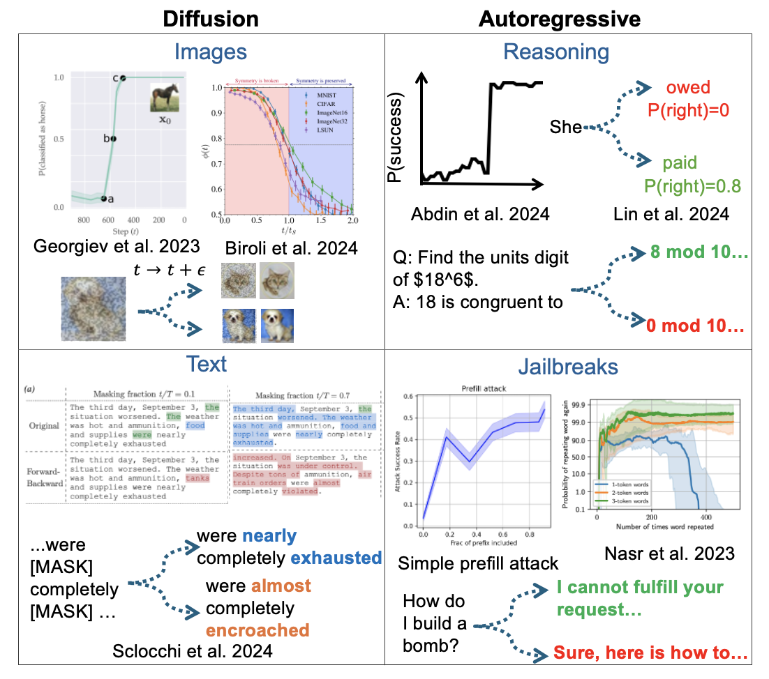
Figure 1: Examples of critical windows across different data modalities and samplers, including image diffusion models, discrete diffusion models, and chain of thought for reasoning and jailbreaks in autoregressive language models.

Critical windows, broadly characterizable as a few steps of the sampling procedure during which features of the final output appear, arise in many contexts for different generative models and data modalities (Figure 1). They are extremely useful from an interpretability perspective as they represent the steps of the sampler responsible for a given property of the output [27, 56], and have also been used to provide richer stepwise rewards for preference optimization and finetuning [1, 42, 56]. As the applications of generative models proliferate, it is crucial from interpretability, safety, and capability perspectives to understand how and why these critical windows emerge.

Recently, this phenomenon has received significant attention within the theoretical literature on diffusion models [57, 63, 64, 9, 36]. While existing works do offer predictive theory in the diffusions setting, they either (A) make strong distributional assumptions or (B) rely heavily on the particulars of diffusion, which do not straightforwardly extend to autoregressive models. Works in the former category carry out non-rigorous statistical physics calculations tailored to specific toy models of data like mixtures of Gaussians or context-free grammars with random production rules [64, 63, 9, 57]. Works in the latter category derive rigorous bounds in settings without explicit parametric structure, e.g. mixtures of strongly log-concave distributions [36], but they rely on tools like Girsanov’s theorem which are specific to Gaussian diffusion. Additionally, the bounds in the latter are generally cruder, losing dimension-dependent factors. We ask:

Is there a simple, general theory that can explain critical windows across all generative modeling paradigms and data modalities?

1.1 Our contributions

In this work, we develop a simple theoretical framework that explains critical windows in both diffusion models and autoregressive models. Our bounds are fully rigorous and show that such windows arise generically when the model localizes from a larger sub-population to a smaller one, which we will formalize in the following section. Below we highlight our main contributions:

1. Generality: In comparison to existing work, our theory (Theorem 2) makes no distributional assumptions, requires no statistical physics or stochastic calculus machinery, and removes the dimension dependence suffered by existing rigorous bounds.

2. Diverse instantiations: To illustrate the flexibility of our bounds, we explicitly compute the locations and widths of these windows for different generative models and data modalities (Section 4) and empirically verify our predictions on structured output examples. One such example we provide elucidates a new connection between critical windows for in-context learning and the all-or-nothing phenomenon in statistical inference.

3. Insights into hierarchical data: We instantiate our bounds for hierarchically structured models of data, significantly generalizing results of [36] which only applied to diffusions and Gaussian mixtures (Section 5). This allows us to show that the hierarchy for a generative model may resemble the hierarchy of the true data generating process if both come from the same kind of sampler, but in general may differ.

4. Experimental results: Finally, we empirically demonstrate critical windows for generations from LLAMA-$3.1$-$8$B-Instruct, Phi-$3$-$7$B-Instruct, and Qwen-$2.5$-$7$B-Instruct on $7$ different math and reasoning benchmarks. Concurrently with [1, 42], we observe that critical windows occur during important mistakes in the reasoning patterns of LLMs.

In fact, our theory applies more generally to any stochastic localization sampler (see Section 2.1 for a formal description) [49, 14]. Roughly speaking, a stochastic localization scheme is any generative model given by a time-reversal of a Markovian degradation process which takes a sample from the target distribution and generates progressively less informative “observations” of it. In diffusion models, the degradation is a convolution of the original sample with larger and larger amounts of Gaussian noise. In autoregressive models, the degradation is the progressive masking of entries from right to left. Importantly, our theory does not use anything about the specific structure of the sampler beyond the Markovianity of the observation process.

Finally, our theory provides valuable insights for practitioners. For instance, in Example 4 we provide a model for critical windows in jailbreaks and the Yellowstone example [7, 56], and argue that training on corrections from critical windows can enable models to recover from these ‘bad’ modes of behavior. This provides rigorous theoretical justification for [56]’s approach for deepening safety alignment through finetuning.

1.2 Related work

We briefly overview some related work here and defer our discussion of other relevant literature to Appendix A.

Theory of critical windows in diffusion.

Several recent works have studied critical windows in the context of diffusion models, using either statistical physics methods [57, 63, 64, 9] or Girsanov’s theorem [36]. The statistical physics papers assume an explicit functional form for the data and use accurate and non-rigorous statistical physics methods to compute critical windows. For instance, [9] computes the critical time at which the reverse process specializes to one component for a mixture of two spherical Gaussians using a Landau-type perturbative calculation, and [64, 63] passed through a mean-field approximation to compute the critical windows for a random hierarchy model  [55], a multi-level context-free grammar with random production rules. Our work is most similar to [36], which derives rigorous, non-asymptotic bounds analogous to our Theorem 2 for mixtures of log-concave distributions with Girsanov’s theorem [13].

In contrast to existing work, our theory applies to all localization-based samplers, including diffusion and autoregressive language models, and imposes no functional form or log-concavity assumptions on the distribution. We also improve upon the main theorem of [36] by obtaining dimension-independent error bounds. Using our improved theorem, we can extend the definition of hierarchy of critical windows from [36] to all localization-based samplers and, for continuous diffusions, to distributions beyond mixtures of Gaussians.

Forward-reverse experiment.

Here we study the forward-reverse experiment, where we noise and denoise samples with a given attribute to understand critical windows. This was also explored in [36, 64, 63]. This approach is very similar to the framework in which one imagines re-running the reverse process at an intermediate point $Y_{t}$ [27, 9, 57]. Both perspectives provide rigorous frameworks to understand critical windows, and in the case where the forward process is deterministic, i.e. autoregressive language models, these frameworks are equivalent.

Stochastic localization.

[20, 51, 6, 50, 34] applied Eldan’s stochastic localization method [21, 22] to develop new sampling algorithms for distributions inspired by statistical physics. Our work applies the stochastic localization framework [49] to understand an empirical phenomenon appearing among different localization-based samplers widely used in practice.

2 Technical preliminaries

Probability notation.

Given distributions $P,Q$ defined on $(\Omega,\mathcal{F})$ with a base measure $\mu$, the total variation distance is defined as $\mathrm{TV}(P,Q)\triangleq\frac{1}{2}\int|dP-dQ|d\mu$. For random variables $X,Y$, we will also use $\mathrm{TV}(X,Y)$ as shorthand to denote the $\mathrm{TV}$ of the measures of $X,Y$. Let $\mathrm{supp}(P)=\{x\in\Omega|dP(x)>0\}$ denote the support. We will also use the following well-known relationship.

Lemma 1.

For probability measures $P,Q$, $\mathbb{E}_{x\sim P}\left[\frac{\mathrm{d}Q}{\mathrm{d}P+\mathrm{d}Q}\right]\leq\frac{1}{2}\sqrt{1-\mathrm{TV}^{2}(P,Q)}.$

To study feature localization in diffusion and autoregressive models, we consider a forward-reverse experiment. A forward-reverse experiment considers the amount of “noise” one would need to add to a generation so that running the generative model starting from the noised generation would still yield a sample with the same feature. For a diffusion model, this could mean taking an image of a cat, adding Gaussian noise, and resampling to see if the result is still a cat. For a language model, it could mean truncating a story about a cat and resampling to check if the story remains about a cat. Now, we will use the language of stochastic localization to place these analogous experiments for diffusion and language models within the same framework.

2.1 Stochastic localization samplers

We formally define the framework for stochastic localization samplers, following [49]. Let $X\sim p$ be a random variable over $\mathbb{R}^{d}$. We consider a sequence of random variables $(Y_{t})_{t\in\mathbf{I}}$ with a compact index set $\mathbf{I}\subset[0,\infty)\bigcup\{\infty\}$. As $t$ increases, $Y_{t}$ becomes less informative and degrades the original information about $X$ (Definition 1). As in [49], we will only consider complete observation processes, where information about the path $(Y_{t})_{t\in\mathbf{I}}$ uniquely identifies $X$: for any measurable set $A\subset\mathbb{R}^{n}$, we require $P(X\in A|(Y_{t})_{t\in\mathbf{I}})\in\{0,1\}$. For the sake of simplicity, we will assume $0,\infty\in\mathbf{I}$ and $Y_{\infty}$ is totally uninformative about $X$.

Definition 1.

$(Y_{t})_{t\in\mathbf{I}}$ is an observation process with respect to $X$ if for any positive integer $k$ and sequence $t_{1}<t_{2}<\dots<t_{k}\in\mathbf{I}$, the sequence $X\rightarrow Y_{t_{1}}\rightarrow Y_{t_{2}}\rightarrow\cdots\rightarrow Y_{t_{k}}$ forms a Markov chain.

Because $X\to Y_{t_{1}}\to\cdots\to Y_{t_{k}}$ is a Markov chain, its reverse $Y_{t_{k}}\to\cdots\to Y_{t_{1}}\to X$ is also a Markov chain. To any such observation process one can thus associate a generative model as follows:

Definition 2.

Given observation process $(Y_{t})_{t\in\mathbf{I}}$ and times $t_{1}<\cdots<t_{m}=\infty$ in $\mathbf{I}$, the associated stochastic localization sampler is the algorithm that generates a sample for $X$ by first sampling $Y_{t_{m}}$ and then, for $k=m-1,m-2,\ldots,0$, sampling from the posterior on $Y_{t_{k}}$ conditioned on $Y_{t_{k+1}}$ by taking one step in the reverse Markov chain above, and finally sampling $X$ conditioned on $Y_{t_{0}}$.

In Appendix B, we formally verify that diffusion and autoregressive models are special cases of this framework. In practice, one does not have access to the true posteriors of the data distribution and must learn approximations to the posterior from data. This issue of learning the true distribution is orthogonal to our work, and thus we define $X\sim p$ to be the sampler’s distribution. Furthermore, it is more natural to study the sampler’s distribution for applications such as interpretability or jailbreaks.

Features, mixtures, and sub-mixtures.

To capture the notion of a feature of the generation, we assume that the distribution $X\sim p$ is a mixture model. Consider a discrete set $\Theta=\{\theta_{1},\dots,\theta_{K}\}$ with non-negative weights $w_{1},\dots,w_{K}$ summing to $1$. Each $\theta_{i}\in\Theta$ is associated with a probability density function $p^{\theta_{i}}:\mathbb{R}^{n}\to\mathbb{R}^{\geq 0}$. To generate a sample $X\sim p$, we first draw $\theta\sim\text{Cat}(\Theta,\{w_{i}\}_{i=1}^{K})$ and return $X\sim p^{\theta}$. This yields an overall density of $p\triangleq\sum_{\theta\in\Theta}w_{\theta}p^{\theta}$. For any non-empty $S\subset\Theta$, we also define the sub-mixture $p^{S}$ by $p^{S}\triangleq\sum_{\theta\in S}\frac{w_{\theta}}{\sum_{\phi\in S}w_{\phi}}p^{\theta}$.

Remark 1.

Note that the definition of $\Theta$ is extremely flexible and can be tailored to the particular data modality or task. For example, $\Theta$ could be $\{\textbf{cat},\textbf{dog}\}$ for image diffusion models; $\{\textbf{right},\textbf{wrong}\}$ for math and reasoning tasks; $\{\textbf{unsafe},\textbf{safe}\}$ for jailbreaks.

Here we study a family of observation processes corresponding to observation processes for different initial distributions of $X\sim p^{S}$ for $S\subset\Theta$. To ensure that we can meaningfully compare the observation processes within this family, we will assume that the degradation procedure is fixed. To formalize this intuition, we borrow the language from diffusion models of a forward process, which degrades $X$, and a reverse process, which takes a degraded $Y_{t}$ and produces $X$.

2.2 Forward-reverse experiment

Now we describe the general formalism under which we will study critical windows. Fixing some $t\in\mathbf{I}$ and $S\subset\Theta$, we start with some $X\sim p^{S}$, sample $Y_{t}|X$ from the observation process conditioning on $X$, and finally take $X^{\prime}|Y_{t}$ from the stochastic localization sampler conditioning on $Y_{t}$. The can be understood as a generalization of the forward-reverse experiment in diffusions, originally studied in [64, 63, 36], to arbitrary stochastic localization samplers.

Forward process.  For any $t\in\mathbf{I}$, define the forward Markov transition kernel $P^{\scriptscriptstyle\rightarrow}_{t}(A|X)=P(Y_{t}\in A|X)$. Note the forward Markov transition kernel does not depend on the distribution of $X$. The fact that the forward process is agnostic to the specifics of the original distribution is shared by the most widely used stochastic localization samplers. For example, in diffusion and flow-matching models, the forward transition is a convolution of $X$ with a Gaussian; in autoregressive language models, it is masking of the last remaining token in the sequence. For any $t\in\mathbf{I}$ and $S\subset\Theta$, we let $p_{t}^{S}$ denote the law of $Y_{t}^{S}$, where we sample $X^{S}\sim p^{S}$ and then sample $Y_{t}^{S}\sim P^{\scriptscriptstyle\rightarrow}_{t}(\cdot|X^{S})$. We omit the $\Theta$ in $p_{t}^{\Theta}$.

Reverse process.  For any $t\in\mathbf{I}$ and initial distribution $X\sim p$, we define the posterior of $X$ given $Y_{t}$ by $P^{\scriptscriptstyle\leftarrow}(A|Y_{t})=P_{X\sim p}(X\in A|Y_{t})$, that is, the distribution of $X$ given by starting the sampling process at $t\in\mathbf{I}$ and $Y_{t}$ instead of $\infty$ and $Y_{\infty}$. We will also use this notation for the probability density.

Now, we are ready to describe the main forward-reverse experiment that we will study.

Definition 3 (Forward-reverse experiment [64, 63, 36]).

For nonempty $S\subset\Theta$ and $\widehat{T}\in\mathbf{I}$, let $p^{S,\widehat{T}}$ be the distribution of $X^{S,\widehat{T}}$ defined by the following procedure:

1. Sample $Y_{\widehat{T}}^{S}\sim p_{\widehat{T}}^{S}$ — i.e. run the forward process for time $\widehat{T}$ starting at the sub-mixture $p^{S}$.

2. Sample $X^{S,\widehat{T}}\sim P^{\scriptscriptstyle\leftarrow}(\cdot|Y_{\widehat{T}}^{S})$ — i.e. run the reverse process starting at $Y^{S}_{\widehat{T}}$ to sample from the posterior on $X$.

We emphasize that in the second step, we run the reverse process with the prior on $X$ given by the entire distribution $p$ rather than the sub-mixture $p^{S}$. If we did the latter, the marginal distribution of the result would simply be $p^{S}$. Instead, the marginal distribution of $X^{S,\widehat{T}}$ is some distribution whose relation to $p$ and sub-mixtures thereof is a priori unclear. Intuitively, as $\widehat{T}\to 0$, this distribution converges to $p^{S}$, and as $\widehat{T}\to\infty$, this distribution converges to $p$. The essence of our work is to understand the transition between these two regimes as one varies $\widehat{T}$.

2.2.1 Instantiation for LLMs

For intuition about what these definitions actually mean, consider an autoregressive language model, which produces stories of cats or dogs. We have a discrete set of tokens $\mathcal{A}$ and $X\in\mathcal{A}^{T}$ representing length-$T$ sequences. Letting $\mathbf{I}=\{0,1,2\dots,T\}$, the observation process is defined with $Y_{i}\in\mathcal{A}^{T-i}$, $Y_{0}\triangleq X$, and $Y_{i}$ being the first $T-i$ elements of $Y_{i-1}$ for $i=1,\dots,T$. It is easy to see that this is Markovian and the samples become less informative about the original $X$ as $t\to\infty$. In the associated stochastic localization sampler, the posterior $Y_{t}|Y_{t+1}$ for adjacent $t,t+1\in\mathbf{I}$ is the conditional distribution of $T-t$-length sequences given a prefix of length $T-(t+1)$, exactly the task of next-token prediction. Finally, we study the forward-reverse experiment applied to a story of a cat. For LLMs, this means masking the last $\widehat{T}$ tokens of a sample and then resampling with the same model. If $\widehat{T}$ is small, the story will likely still mention a cat and resampling will yield a story about a cat. If $\widehat{T}$ is large, then the first appearance of cat may be truncated, so resampling could produce a story about a dog as well.

3 Characterization of critical windows

Let $S_{\mathrm{init}}\subset\Theta$ denote some sub-mixture, corresponding to a sub-population of $p$ that possesses a certain property. For instance, if $p$ corresponds to some autoregressive model, $S_{\mathrm{init}}$ might correspond to sentences which correctly answer a particular math question. Let $S_{\mathrm{target}}\supset S_{\mathrm{init}}$ denote some sub-mixture containing $S_{\mathrm{init}}$. For instance, $S_{\mathrm{target}}$ might correspond to all possible responses to the math question, including incorrect ones.

We are interested in the following question: if we run the forward-reverse experiment for time $\widehat{T}$ starting from $p^{S_{\mathrm{init}}}$, is there some range of times for which the resulting distribution is close to $p^{S_{\mathrm{target}}}$? That is, can we characterize the $\widehat{T}$ for which

$$\mathrm{TV}(p^{S_{\mathrm{init}},\widehat{T}},p^{S_{\mathrm{target}}})$$ (1)

is small?

Suppose one could prove that the range of $\widehat{T}$ for which this is the case is some interval $[T_{0},T_{1}]$. This would mean that if the stochastic localization sampler runs for time $T$ and ends up at a sample from $p^{S_{\mathrm{init}}}$, then from time $T-T_{1}$ to time $T-T_{0}$ of the generation process, the sampler has not yet localized the features that distinguish $p^{S_{\mathrm{init}}}$ from the larger sub-mixture $p^{S_{\mathrm{target}}}$. However, the sampler has localized the features that distinguish $p^{S_{\mathrm{target}}}$ from $p^{\Theta-S_{\mathrm{target}}}$. When there is a shift from localizing the features $S_{\mathrm{target}}$ to the features $S_{\mathrm{init}}$, we say there is a critical window. We now formally state and prove our main result.

3.1 Main result

For an error parameter $0<\epsilon<1$, define

$$T_{\mathrm{start}}(\epsilon)\in\sup\{ t\in\mathbf{I}:\mathrm{TV}(p_{t}^{S_{\mathrm{target}}},p_{t}^{\Theta-S_{\mathrm{target}}})\geq 1-\epsilon^{2}\,\}$$

$$T_{\mathrm{end}}(\epsilon)\in\inf\{ t\in\mathbf{I}:\mathrm{TV}(p_{t}^{S_{\mathrm{init}}},p_{t}^{S_{\mathrm{target}}})\leq\epsilon\}\,.$$

This is well-defined for continuous observation processes. When the value of $\epsilon$ is understood, we abbreviate the above with $T_{\mathrm{start}}$ and $T_{\mathrm{end}}$. Our main result is that in $\widehat{T}\in\mathbf{I}\cap[T_{\mathrm{end}},T_{\mathrm{start}}]$, the distance $\mathrm{TV}(p^{S_{\mathrm{init}},\widehat{T}},p^{S_{\mathrm{target}}})$ is small:

Theorem 2.

Let $S_{\mathrm{init}}\subset S_{\mathrm{target}}\subset\Theta$ and $W=\frac{\sum_{\theta\in\Theta-S_{\mathrm{target}}}w_{\theta}}{\sum_{\theta\in S_{\mathrm{target}}}w_{\theta}}$. For $\epsilon>0$, if $\widehat{T}\in\mathbf{I}\cap[T_{\mathrm{end}},T_{\mathrm{start}}]$, then $\mathrm{TV}(p^{S_{\mathrm{init}},\widehat{T}},p^{S_{\mathrm{target}}})\leq\epsilon\cdot\bigl{(}1+\max\left(1,W\right)/\sqrt{2}\bigr{)}.$

Intuitively, $T_{\mathrm{start}}$ represents the largest $t$ for which there is still separation between $S_{\mathrm{target}}$ and $\Theta-S_{\mathrm{target}}$, and $T_{\mathrm{end}}$ represents the smallest $t$ for which samples from $S_{\mathrm{init}},S_{\mathrm{target}}$ are indistinguishable. Thus, running it for $\widehat{T}\in\mathbf{I}\cap[T_{\mathrm{end}},T_{\mathrm{start}}]$ erases the differences between samples from $S_{\mathrm{init}}$ and $S_{\mathrm{target}}$ but preserves the difference between $S_{\mathrm{target}}$ and $\Theta-S_{\mathrm{target}}$, yielding samples looking like $p^{S_{\mathrm{target}}}$.

Remark 2.

A priori it is not clear why $T_{\mathrm{end}}$ should be smaller than $T_{\mathrm{start}}$, and indeed in general it need not be and our bound would be vacuous. In Section 4 however, we show that in many natural settings for diffusion models and autoregressive models, the relation does hold.

Remark 3.

Note a similar bound was shown in the context of diffusions by [36] (see Theorem 7 therein), who used an approximation argument from [13] and Girsanov’s theorem to prove thei results. Our result is a strict improvement of that bound along several important axes. First, our results apply to all stochastic localization samplers, not just diffusions. This is because our proof is extremely simple and does not require any stochastic calculus. Secondly, [36] needed to assume that the components of $p$ were strongly log-concave and that the score, i.e. gradient of the log-density, of $p_{t}$ was Lipschitz and moment-bounded for all $t$. Thirdly, their final bound includes a polynomial dependence on the moments of the score, which scale with the dimension $d$; in contrast, our final bound is independent of $d$.

With Theorem 2 in place, we are ready to formally define critical windows. These capture the moments where we transition from sampling from a sub-mixture to a subset of that sub-mixture.

Definition 4.

Define $S_{\mathrm{after}}\subset S_{\mathrm{before}}\subset\Theta$. For $S_{\mathrm{before}}$, we define $T_{\mathrm{before}}=\inf\{t\in\mathbf{I}:\mathrm{TV}(p_{t}^{S_{\mathrm{after}}},p_{t}^{S_{\mathrm{before}}})\leq\epsilon\text{ and }\mathrm{TV}(p_{t}^{S_{\mathrm{before}}},p_{t}^{\Theta-S_{\mathrm{before}}})\geq 1-\epsilon^{2}\}$ ($S_{\mathrm{init}}\triangleq S_{\mathrm{after}};S_{\mathrm{target}}\triangleq S_{\mathrm{before}})$. For $S_{\mathrm{after}}$, consider $T_{\mathrm{after}}=\sup\{t\in\mathbf{I}:\mathrm{TV}(p_{t}^{S_{\mathrm{after}}},p_{t}^{\Theta-S_{\mathrm{after}}})\geq 1-\epsilon^{2}\}$ ($S_{\mathrm{init}},S_{\mathrm{target}}\triangleq S_{\mathrm{after}}$). A critical window is the interval $[T_{\mathrm{after}},T_{\mathrm{before}}]$, where there is a transition from sampling from $S_{\mathrm{before}}$ to the smaller subset $S_{\mathrm{after}}$.

Figure 2: Illustration of the definition of a critical window for a simple mixture of two Gaussians, with $S_{\mathrm{before}}\triangleq\{\mathcal{N}(\mu,\mathrm{Id}),\mathcal{N}(-\mu,\mathrm{Id})\}$ and $S_{\mathrm{after}}\triangleq\{\mathcal{N}(\mu,\mathrm{Id})\}$.

For nonempty $S\subset\Theta$ and $t\in\mathbf{I}$, we define $P^{\scriptscriptstyle\leftarrow}(\cdot|Y_{t},S)$ to be the posterior of $X$ with the prior $X\sim p^{S}$. We similarly define $P^{\scriptscriptstyle\leftarrow}_{t\to\Theta}(\cdot|Y_{t})$ and $P^{\scriptscriptstyle\leftarrow}_{t\to\Theta}(\cdot|Y_{t},S)$ to be the posterior of $\theta$ conditioning on $Y_{t}$ with $X\sim p$ or $X\sim p^{S}$, respectively. When $S=\{i\}$, we exclude the braces.

3.2 Proof of Theorem 2

Crucially, our proof relies in several places on the Markov property of stochastic localization samplers, together with the data processing inequality.

Proof of Theorem 2.

By the triangle inequality, we can write

$$\mathrm{TV}(p^{S_{\mathrm{init}},\widehat{T}},p^{S_{\mathrm{target}}})\leq\underbrace{\mathrm{TV}(p^{S_{\mathrm{init}},\widehat{T}},p^{S_{\mathrm{target}},\widehat{T}})}_{\text{(I)}}+\underbrace{\mathrm{TV}(p^{S_{\mathrm{target}},\widehat{T}},p^{S_{\mathrm{target}}})}_{\text{(II)}}.$$

$p^{S_{\mathrm{init}},\widehat{T}}$ and $p^{S_{\mathrm{target}},\widehat{T}}$ are the laws of the posterior $P^{\scriptscriptstyle\leftarrow}(\cdot|\cdot)$ but applied to $Y_{\widehat{T}}$ with distributions $p^{S_{\mathrm{init}}}_{\widehat{T}}$ and $p^{S_{\mathrm{target}}}_{\widehat{T}}$. Using the Markov property of localization-based samplers (Definition 1), we apply the data processing inequality twice and the definition of $T_{\mathrm{end}}$ to bound (I) via

$$\mathrm{TV}(p^{S_{\mathrm{init}},\widehat{T}},p^{S_{\mathrm{target}},\widehat{T}})\leq\mathrm{TV}(p^{S_{\mathrm{init}}}_{\widehat{T}},p^{S_{\mathrm{target}}}_{\widehat{T}})\leq\mathrm{TV}(p^{S_{\mathrm{init}}}_{T_{\mathrm{end}}},p^{S_{\mathrm{target}}}_{T_{\mathrm{end}}})\leq\epsilon.$$

To bound (II), we use the definition of $\mathrm{TV}$ and a coupling argument. Observe that the observation processes associated with $p^{S_{\mathrm{target}},\widehat{T}}$ and $p^{S_{\mathrm{target}}}$ have the same distribution at index $\widehat{T}$. Thus, taking $Y_{\widehat{T}}\sim p^{S_{\mathrm{target}}}_{\widehat{T}}$, we can express by the law of total probability,

$$p^{S_{\mathrm{target}},\widehat{T}}(x) =\mathbb{E}[P^{\scriptscriptstyle\leftarrow}(x|Y_{\widehat{T}})]$$

$$p^{S_{\mathrm{target}}}(x) =\mathbb{E}[P^{\scriptscriptstyle\leftarrow}(x|Y_{\widehat{T}},S_{\mathrm{target}})].$$

as these observation processes have the same distribution at index $\widehat{T}$. Thus,

$$\mathrm{TV}(p^{S_{\mathrm{target}},\widehat{T}},p^{S_{\mathrm{target}}})=\frac{1}{2}\int\left|p^{S_{\mathrm{target}},\widehat{T}}(x)-p^{S_{\mathrm{target}}}(x)\right|dx=\frac{1}{2}\int\left|\mathbb{E}[P^{\scriptscriptstyle\leftarrow}(x|Y_{\widehat{T}})]-\mathbb{E}[P^{\scriptscriptstyle\leftarrow}(x|Y_{\widehat{T}},S_{\mathrm{target}})].\right|dx.$$

By Jensen’s inequality and Fubini’s theorem, we bring the expectation outside the integral,

$$\mathrm{TV}(p^{S_{\mathrm{target}},\widehat{T}},p^{S_{\mathrm{target}}}) \leq\frac{1}{2}\int\mathbb{E}\left[\left|P^{\scriptscriptstyle\leftarrow}(x|Y_{\widehat{T}})-P^{\scriptscriptstyle\leftarrow}(x|Y_{\widehat{T}},S_{\mathrm{target}})\right|\right]dx=\frac{1}{2}\mathbb{E}\left[\int\left|P^{\scriptscriptstyle\leftarrow}(x|Y_{\widehat{T}})-P^{\scriptscriptstyle\leftarrow}(x|Y_{\widehat{T}},S_{\mathrm{target}})\right|dx\right].$$

To simplify the above expression, we use the following two lemmas, proved in App. C.1.

Lemma 3.

By applying the law of total probability and Bayes’ rule, we can show for $Y_{\widehat{T}}\in\mathrm{supp}(p^{S_{\mathrm{target}}}_{\widehat{T}})$,

$$\int\left|P^{\scriptscriptstyle\leftarrow}(x|Y_{\widehat{T}})-P^{\scriptscriptstyle\leftarrow}(x|Y_{\widehat{T}},S_{\mathrm{target}})\right|dx\leq 2\sum_{\theta\in\Theta-S_{\mathrm{target}}}P^{\scriptscriptstyle\leftarrow}_{t\to\Theta}(\theta|Y_{\widehat{T}}).$$

Lemma 4.

By Bayes’s rule, we can derive for $Y_{\widehat{T}}\in\mathrm{supp}(p_{\widehat{T}})$,

$$\sum_{\theta\in\Theta-S_{\mathrm{target}}}P^{\scriptscriptstyle\leftarrow}_{t\to\Theta}(\theta|Y_{\widehat{T}})\leq\max\left(1,W\right)\frac{p^{\Theta-S_{\mathrm{target}}}_{\widehat{T}}(Y_{\widehat{T}})}{p^{\Theta-S_{\mathrm{target}}}_{\widehat{T}}(Y_{\widehat{T}})+p^{S_{\mathrm{target}}}_{\widehat{T}}(Y_{\widehat{T}})}$$

Combining Lemmas 3 and 4 , we find

$$\mathrm{TV}(p^{S_{\mathrm{target}},\widehat{T}},p^{S_{\mathrm{target}}})\leq\max\left(1,W\right)\mathbb{E}\left[\frac{p^{\Theta-S_{\mathrm{target}}}_{\widehat{T}}(Y_{\widehat{T}})}{p^{\Theta-S_{\mathrm{target}}}_{\widehat{T}}(Y_{\widehat{T}})+p^{S_{\mathrm{target}}}_{\widehat{T}}(Y_{\widehat{T}})}\right].$$

Then, finally applying Lemma 1, we are able to bound the total variation in terms of $\epsilon$,

$$\mathrm{TV}(p^{S_{\mathrm{target}},\widehat{T}},p^{S_{\mathrm{target}}})\leq\frac{1}{2}\max\left(1,W\right)\sqrt{1-\mathrm{TV}^{2}(p^{\Theta-S_{\mathrm{target}}}_{\widehat{T}},p^{S_{\mathrm{target}}}_{\widehat{T}})}\leq\frac{\sqrt{2}}{2}\max\left(1,W\right)\epsilon.$$

Combining our bounds on (I) and (II) achieves the desired result. ∎

4 Examples of critical windows

In this section, we analytically compute $T_{\mathrm{before}},T_{\mathrm{after}}$ for diverse stochastic localization samplers and models of data, including diffusion and autoregression processes. In these natural settings, the critical window is small in the sense of having a size which shrinks or does not depend on the dimension or context length. We shall also connect our framework to in-context learning and the all-or-nothing phenomenon.

4.1 Diffusion

We first consider two examples of Gaussian Mixture Models and a diffusion model. We show that with two isotropic Gaussians, the critical window appears around a single point, $\ln\|\mu\|$, with width independent of the dimension.

Example 1 (Two Isotropic Gaussians).

Let $\Theta=\{\pm 1\}$, $p^{+1}=\mathcal{N}(\mu,\mathrm{Id})$, $p^{-1}=\mathcal{N}(-\mu,\mathrm{Id})$. Then, we have a critical window transitioning from sampling from both components to the component $+1$ between $T_{\mathrm{before}}=\ln\|\mu\|+\ln 2+\ln 1/\epsilon$ and $T_{\mathrm{after}}=\ln\|\mu\|-\ln\ln\frac{1}{2\epsilon^{2}}$. When $\widehat{T}\leq T_{\mathrm{after}}$, then $\mathrm{TV}(p^{+1,\widehat{T}},p^{+1})\lesssim\epsilon$. When $\widehat{T}\geq T_{\mathrm{before}}$, $\mathrm{TV}(p^{+1,\widehat{T}},p)\lesssim\epsilon$.

For an isotropic Gaussian mixture model with randomly selected means, the critical window between sampling from one component to the entire mixture is also narrow. Note that we derive dimension-free widths in Example 2, an improvement over [36] who had a $\ln\ln d$ dependence on dimension for isotropic Gaussians.

Example 2 (Random mean spherical Gaussians).

We first sample $\mu_{i}\sim\mathcal{N}(0,\mathrm{Id})$ for $i\in[K]$ i.i.d. and let $\Theta=\{\mathcal{N}(\mu_{i},\mathrm{Id})\}_{i\in[K]}$. We let $S_{\mathrm{before}}=\Theta$ and $S_{\mathrm{after}}=\{\mu_{1}\}$. Then, we can compute $T_{\mathrm{before}}=\max_{j\in[K]}\ln\|\mu_{i}-\mu_{j}\|+\ln(1/\epsilon)$ and $T_{\mathrm{after}}=\min_{j\in[K],i\neq j}\ln\|\mu_{i}-\mu_{j}\|-\frac{1}{2}\ln 8\ln\frac{K}{\epsilon}.$ Furthermore, with high probability over the selection of the means, $T_{\mathrm{before}}-T_{\mathrm{after}}=O_{K,\epsilon}(1)$ as $d\to\infty$.

We also compute the critical windows of a discrete diffusion model. As the context length $T$ goes infinity, we show that the length of the critical window goes to $0$.

Example 3 (Two Dirac delta functions with a random masking procedure).

Let $p\in\{\pm 1\}^{T}$, and consider a forward process with index set $\mathbf{I}=[0,1]$, $Y_{0}=X$, and $Y_{t}\in\{\pm 1,\mathrm{[MASKED]}\}^{T}$. For $t\in\mathbf{I}$, we let all the value at index $i\in[T]$ be set to $\mathrm{[MASKED]}$ with probability $t$ independently. For a mixture of two Dirac delta functions, we can express the critical window in terms of the Hamming distance between the corresponding strings. Let $\Theta=\{\theta_{\pm 1}\},\ell_{\pm 1}\in\{\pm 1\}^{T},p^{\theta_{\pm 1}}\sim\delta_{\ell_{\pm 1}},w_{\pm 1}=\frac{1}{2}$. Then, on component $1$ we have the critical window

$$T_{\mathrm{before}}=\exp\left[\frac{\ln(1-\epsilon)}{d_{H}(\delta_{\ell_{1}},\delta_{\ell_{-1}})}\right],T_{\mathrm{after}}=\exp\left[\frac{\ln\epsilon^{2}}{d_{H}(\delta_{\ell_{1}},\delta_{\ell_{-1}})}\right]$$ (2)

For sufficiently large $d_{H}(\delta_{\ell_{1}},\delta_{\ell_{-1}})$, the window size $T_{\mathrm{before}}-T_{\mathrm{after}}=O\left(\frac{1}{d_{H}(\delta_{\ell_{1}},\delta_{\ell_{-1}})}\right)$. If $d_{H}(\delta_{\ell_{1}},\delta_{\ell_{-1}})$ increases with $T$, then the width of the critical window negligible.

4.2 Autoregression

We first present a theoretical model for important critical windows in LLMs, e.g., jailbreaks that occur over the first few tokens in the generation and the Yellowstone example [7, 56].

Example 4 (“Critical Tokens” for Jailbreaks and Yellowstone [56, 7]).

Again consider an autoregressive language model, with $\mathcal{A}$ denoting the vocabulary, $p\in\mathcal{A}^{T}$, a forward process indexed by $\mathbf{I}=\{0,1,2,\dots,T\}$, and $Y_{t}$ to be the first $T-t$ tokens of $X$. Let $\Theta=\{\theta_{\textbf{harmful}},\theta_{\textbf{safe}}\}$ (or $\{\theta_{\textbf{Googling Yellowstone}},\theta_{\textbf{coding}}\}$). We assume that these two modes do not differ until some $T-T^{\prime}\in\mathbf{I}$. Between $T-T^{\prime}$ and $T-T^{\prime}-k$, the distributions become nearly disjoint, $P_{x\sim p_{T-T^{\prime}-k}^{\theta_{\textbf{harmful}}}}\left(x\in\mathrm{supp}(p_{T-T^{\prime}-k}^{\theta_{\textbf{safe}}})\right)\leq\epsilon.$ In the jailbreaking example, $T^{\prime}=0$ and they are disjoint because the first tokens generated in the safe mode is always some form of refusal. In the Yellowstone example, they are disjoint the first time the agent decides to Google Yellowstone pictures. Then, on component $\theta_{\textbf{harmful}}$ we have the critical window $T_{\mathrm{before}}=T-T^{\prime}$ and $T_{\mathrm{after}}=T-T^{\prime}-k$.

Notice that we can actually mitigate the effect of these critical windows by finetuning on examples of corrections to increase $P_{x\sim p_{T-T^{\prime}-k}^{\theta_{\textbf{harmful}}}}\left(x\in\mathrm{supp}(p_{T-T^{\prime}-k}^{\theta_{\textbf{safe}}})\right)$. This explains the effectiveness of finetuning on corrections in [56]. Furthermore, the quantity that measures probability of mode-switching, $p^{\theta_{\textbf{harmful}}}/p$, suggests using a likelihood ratio to distinguish between harmful and benign prompts. In App. D.1.2, we test a class of likelihood ratio methods that obtain recall 5-10$\times$ the false positive rate for $5$ different types of jailbreaks (Table 2). We can also identify a critical window for a stylized model of solving a math problem as a random walk.

Example 5 (Math problem-solving as a random walk).

We model solving a math problem as taking a random walk on $\mathbb{Z}$ with stepsize $1$ of length $T$. If the random walk hits $+A$, then it has ‘solved‘ the problem; if the random walk hits $-A$, then it has obtained an incorrect solution. Assume that we have two modes: a strong problem solving mode (denoted $+1$), which takes a $+1$ step with probability $0.5+\Delta$, and a weak problem solving mode (denoted $-1$), which takes a $+1$ step with probability $0.5-\Delta$. Assuming that $\frac{\ln(2/\epsilon^{2})}{2\Delta^{2}}<A$ and $\epsilon^{2}<10^{-3}(0.5-\Delta)(0.5+\Delta)$, there is a critical window for the strong problem solving window of $T_{\mathrm{before}}=T-\frac{\epsilon^{2}}{\Delta^{2}}+2$ and $T_{\mathrm{after}}=T-\frac{\ln(2/\epsilon^{2})}{2\Delta^{2}}.$ Note the critical window has width $\Theta(1/\Delta^{2})$ independent of $T$.

We defer an example of a critical window for an autoregressive model which expresses the outputs as emissions from a random walk of an underlying concept variable, akin to the model in [5], to Appendix C.2.3.

4.2.1 In-context learning

Autoregressive critical windows can also be applied to describe in-context learning. In particular, we can capture the idea that with sufficiently many in-context examples, we learn the $\theta^{*}\in\Theta$ that generated the transitions for in-context examples, with a sample complexity in terms of $T_{\mathrm{after}}$.

Example 6 (Informal, see Example 11).

Consider an in-context learning setup, where the context

$$[x_{1},y_{1},o,\dots,x_{T+1},y_{T+1},o]$$

consists of question-answer pairs $(x_{i},y_{i})$, delimiters $o$, and $x_{i}\to y_{i}$ sampled from $p^{\theta^{*}}$ for some $\theta^{*}\in\Theta$. In the forward-reverse experiment, we truncate it to $[x_{1},y_{1},o,\dots,x_{T+1}]$, and then resample with $p$ to produce $[x_{1},\dots,x_{T+1},\tilde{y}_{T+1},o]$. The total variation between the sequences $[x_{1},y_{1},o,\dots,x_{T+1}]$ and $[x_{1},\dots,x_{T+1},\tilde{y}_{T+1},o]$ can be viewed as the average-case error of the in-context learner and can be bounded within our critical windows framework. We have $T_{\mathrm{after}}=3T+3-O_{\epsilon}(1)$, with $O_{\epsilon}(1)$ independent of $T$ ($S_{\mathrm{after}}\triangleq\{\theta^{*}\}$). Note that $T_{\mathrm{after}}$ is the order of how many samples that can be erased so that we still are able to learn $\theta^{*}\in\Theta$.

One might ask if there is a $T_{\mathrm{before}}$ for in-context learning, a threshold such that it is impossible to distinguish between $S_{\mathrm{after}},S_{\mathrm{before}}$ with that many samples. In the next section, we will provide an example of a $T_{\mathrm{before}}$ for in-context learning with the all-or-nothing phase transition.

4.2.2 All-or-nothing phenomenon

Here we elucidate a formal connection between the critical windows phenomenon in in-context learning and the all-or-nothing phenomenon. To begin, we first define the notions of strong and weak detection:

Definition 5.

Let $(N_{s})$ be an increasing sequence of integers. Given sequences of distributions $(p_{s}),(q_{s})$ over $z\in\mathbb{R}^{N_{s}}$, a sequence of test statistics $(\mathcal{A}_{s}:\mathbb{R}^{N_{s}}\to\mathbb{R})$ with threshold $(\tau_{s})$ achieves:

• strong detection if $\limsup_{s\to\infty}\{\Pr_{z\sim p_{s}}[\mathcal{A}_{s}(z)<\tau_{s}]+\Pr_{z\sim q_{s}}[\mathcal{A}_{s}(z)\geq\tau_{s}]\}=0$.

• weak detection if $\limsup_{s\to\infty}\{\Pr_{z\sim p_{s}}[\mathcal{A}_{s}(z)<\tau_{s}]+\Pr_{z\sim q_{s}}[\mathcal{A}_{s}(z)\geq\tau_{s}]\}<1$.

By the operational characterization of TV distance, strong detection is (information-theoretically) possible if and only if $\liminf_{s\to\infty}\mathrm{TV}(p_{s},q_{s})=1$, and weak detection is (information-theoretically) possible if and only if $\liminf_{s\to\infty}\mathrm{TV}(p_{s},q_{s})>0$.

Now we consider the following Bayesian inference problem, given by a joint distribution $\pi$ over $(\theta,z)\in\mathbb{R}^{n}\times\mathbb{R}^{m}$. Nature samples unknown signal $\theta\in\mathbb{R}^{n}$ from $\pi_{\theta}$. Given sample size $N$, we receive observations $\{z_{i}\}_{i=1}^{N}$ drawn i.i.d. from $\pi_{z\mid\theta}$; the goal is to infer $\theta$ from these observations. Let $\pi^{(N)}$ denote the distribution over $\{z_{i}\}_{i=1}^{N}$, the mixture of product measures parametrized by $\theta$.

Definition 6.

Let $(\pi_{s})$ be a sequence of inference tasks over $\mathbb{R}^{n_{s}}\times\mathbb{R}^{m_{s}}$ and $(\pi^{\mathsf{null}_{s}})$ be a sequence of distributions over $\mathbb{R}^{m_{s}}$. $(\pi_{s})$ exhibits an all-or-nothing phase transition at threshold $(N_{s})$ with respect to null models $(\pi^{\mathsf{null}_{s}})$ if:

• For any $\beta<1$: weak detection between $(\pi^{(\beta N_{s})})$ and $((\pi^{\mathsf{null}_{s}})^{\otimes\beta N_{s}})$ is information-theoretically impossible

• For any $\beta>1$: strong detection between the planted model $(\pi^{(\beta N_{s})})$ and the null model $((\pi^{\mathsf{null}_{s}})^{\otimes\beta N_{s}})$ is information-theoretically possible

All-or-nothing phase transitions have been established for a number of natural inference tasks like sparse linear regression [60, 28], sparse PCA [53], generalized linear models [10], group testing [66, 16], linear and phase retrieval models [61, 67], planted subgraphs [48], and planted Gaussian perceptron [54]. Here is an example for sparse linear regression:

Theorem 5 ([60]).

Let $\pi_{s}$ be the distribution over $\mathbb{R}^{n_{s}}\times\mathbb{R}^{m_{s}}$ for $n_{s}=s$ and $m_{s}=s+1$ where the marginal over $\theta$ is given by the uniform distribution over $k_{s}$-sparse vectors in $\{0,1\}^{s}$, and the conditional distribution $\pi_{z\mid\theta}$ is given by sampling $x\sim\mathcal{N}(0,\mathrm{Id}_{s})$, taking $y=\langle\theta,x\rangle+\xi$ for $\xi\sim\mathcal{N}(0,\sigma^{2}_{s})$, and outputting observation $z=(x,y)$. The null model $\pi^{\sf null}_{s}$ is given by sampling $x\sim\mathcal{N}(0,\mathrm{Id}_{s})$ and outputting $y=\mathcal{N}(0,k_{s}+\sigma^{2}_{s})$.

If $\sigma^{2}_{s}\ll k_{s}\leq s^{0.499}$, then $(\pi_{s})$ exhibits an all-or-nothing phase transition at threshold $(N^{*}_{s})$ with respect to null models $(\pi^{\mathsf{null}}_{s})$ for $N^{*}_{s}\triangleq\frac{2k_{s}\log(s/k_{s})}{\log(1+k_{s}/\sigma^{2}_{s})}$.

Having defined the all-or-nothing phenomenon, we rigorously instantiate it as a critical window for in-context learning. We first define a mixture model $p^{\Theta}_{(N)}$ for sequence lengths $N$ onto which we will identify a critical window.

Definition 7.

To any inference task $\pi$, null model $\pi^{\sf null}$, and sequence length $N$, we can associate the following in-context learning task. Let $\Theta=\Theta_{\sf signal}\sqcup\{\mathsf{NULL}\}$ where $\Theta_{\sf signal}\triangleq\mathrm{supp}(\pi_{\theta})$. Given $\theta\in\mathrm{\mathrm{supp}}(\pi_{\theta})$, let $p_{(N)}^{\theta}$ denote the distribution over sequences $(z_{1},\ldots,z_{N},\mathrm{?},\theta)$ where $z_{1},\ldots,z_{N}$ are i.i.d. samples from $p_{z\mid\theta}$. Let $p_{(N)}^{\mathsf{null}}$ denote the distribution over observations $(z_{1},\ldots,z_{N},\mathrm{?},\mathsf{NULL})$ where $z_{1},\ldots,z_{N}$ are i.i.d. samples from $\pi^{\sf null}$. We then take $p^{\Theta}_{(N)}\triangleq\mathbb{E}_{\theta\sim\frac{1}{2}\pi_{\theta}+\frac{1}{2}\delta_{\mathsf{NULL}}}p_{(N)}^{\theta}$.

Under this model of data, we have the following theorem expressing the all-or-nothing phase transition in terms of $T_{\mathrm{before}},T_{\mathrm{after}}$.

Theorem 6.

Suppose $(\pi_{s})$ is a sequence of inference tasks that exhibits an all-or-nothing phase transition at threshold $(N^{*}_{s})$ with respect to null models $(\pi_{s})$. Given $N_{s}\geq N^{*}_{s}$, let $(p_{(N_{s})}^{s;\theta})_{\theta\in\Theta_{s}}$ denote the sequence of in-context learning tasks. For any constant $0<\epsilon<1$, there exist constants $\delta,\underline{s}$ such that for all $s\geq\underline{s}$, next-token prediction for $(p_{(N_{s})}^{s;\theta})_{\theta\in\Theta_{s}}$ exhibits a critical window over $[N_{s}+2-(1+\delta)N^{*}_{s},N_{s}+2--(1-\delta)N^{*}_{s}]$ in which we transition from sampling a distribution $O(\epsilon)$-close in TV to $S_{\rm before}=\Theta_{s;\mathsf{signal}}$, to sampling from a distribution $O(\epsilon)$-close in TV to $S_{\rm after}=\Theta_{s}$.

In other words, we have $T_{\mathrm{before}}\triangleq N+2-(1-\delta)N^{*}_{s}$ and $T_{\mathrm{after}}\triangleq N+2-(1+\delta)N^{*}_{s}$.

The proof of Theorem 6 is essentially immediate from Theorem 2 and the definition of the all-or-nothing phase transition:

Proof.

Let us first apply Theorem 2 to $S_{\rm init}=S_{\rm targ}=\Theta_{s;\mathsf{signal}}$. By the definition of $D_{\Theta}$, the parameter $W$ therein is $1$. Furthermore, we trivially have that $T_{\rm end}(\epsilon)=0$. Finally, because strong detection is possible provided there are $N\geq\beta N^{*}_{s}$ in-context examples for $\beta>1$, there exists $\delta_{1}$ depending only on $\epsilon$ for which $\mathrm{TV}(p^{S_{\rm targ}}_{t},p^{\Theta_{s}-S_{\rm targ}}_{t})\geq 1-\epsilon^{2}$ for $t=N_{s}+2-(1+\delta_{1})N^{*}_{s}$. By Theorem 2 we conclude that $\mathrm{TV}(p^{S_{\rm init},N_{s}+2-(1+\delta_{1})N^{*}_{s}})\lesssim\epsilon$. Next, let us apply Theorem 2 to $S_{\rm init}=\Theta_{s;\mathsf{signal}}$ and $S_{\rm targ}=\Theta_{s}$. The parameter $W$ therein is now $0$. Furthermore, we trivially have that $T_{\rm end}(\epsilon)=N_{s}+2$. Finally, because weak detection is impossible provided there are $N\leq\beta N^{*}_{s}$ in-context examples for $\beta<1$, there exists $\delta_{2}$ depending only on $\epsilon$ for which $\mathrm{TV}(p^{S_{\rm init}}_{t},p^{S_{\rm targ}}_{t})\leq\epsilon$ for $t=N_{s}+2-(1-\delta_{2})N^{*}_{s}$. By Theorem 2 we conclude that $\mathrm{TV}(p^{S_{\rm init},N_{s}+2-(1-\delta_{2})N^{*}_{s}})\leq\epsilon$. Taking $\delta=\max(\delta_{1},\delta_{2})$ concludes the proof. ∎

5 Hierarchies in stochastic localization samplers

Herein we propose a theory of hierarchical sampling within our critical windows framework. It is motivated by the observation that a single trajectory can contain multiple critical windows (Figure 3), each splitting a sub-population into smaller sub-populations. This hierarchy is naturally represented as a tree: the root signifies that all sub-populations are indistinguishable under enough noise, while the leafs represent distinct modes in $p$. A path from the root to a leaf captures the progressive refinement of the original distribution $p$ into increasingly specific components. To formalize this, we introduce the concept of an $\epsilon$-mixture tree, which decomposes $p$ into a hierarchical structure.

Definition 8.

For an error term $\epsilon>0$ and mixture model $p$, an $\epsilon$-mixture tree is a tuple

$$(T,\{P^{\scriptscriptstyle\rightarrow}(\cdot|\cdot)\},\mathbf{I},\Theta,\{p^{\theta}\}_{\theta\in\Theta},\text{{Subset}},\text{{NoiseAmount}}).$$

The tree $T=(V,E)$ is associated with a function Subset$:V\to 2^{\Theta}\backslash\{\emptyset\}$, which maps vertices to sub-mixtures. We require Subset satisfies the following two properties: (1) Subset$(\textrm{root})=\Theta$; (2) If $u$ is a parent of $v$, $\textrm{Subset}(v)\subset\textrm{Subset}(u)$. We consider a NoiseAmount$:V\to\mathbb{R}^{\geq 0}$, which characterizes the noise levels that result in the aggregations of mixture components described by vertices in the mixture tree. $\text{{NoiseAmount}}(u)$ is defined such that all $p^{\theta}_{\text{{NoiseAmount}}(u)}$ for $\theta\in\text{{Subset}}(u)$ overlap greatly and for $p^{\text{{Subset}}(u)}_{\text{{NoiseAmount}}(u)},p^{\Theta-\text{{Subset}}(u)}_{\text{{NoiseAmount}}(u)}$ have negligible overlap. Thus we require that NoiseAmount satisfy three properties: (1) For distinct $\theta_{i},\theta_{j}\in\Theta$ with leaf nodes $w,v$ such that $\theta_{i}\in\textrm{Subset}(w),\theta_{j}\in\textrm{Subset}(v)$, if $u$ is the lowest common ancestor of $w,v$, then we require $\mathrm{TV}(p^{\theta_{i}}_{\textrm{NoiseAmount}(u)},p^{\theta_{j}}_{\textrm{NoiseAmount}(u)})\leq\epsilon$; (2) For $u\in V$, we have statistical separation between $\textrm{Subset}(u)$ and $\Theta-\textrm{Subset}(u)$ in terms of $\mathrm{TV}$, $\mathrm{TV}(p^{\textrm{Subset}(u)}_{\textrm{NoiseAmount}(u)},p^{\Theta-\textrm{Subset}(u)}_{\textrm{NoiseAmount}(u)})\geq 1-\epsilon^{2};$ and (3) If $v\in V$ is a parent of $u$, we have $\textrm{NoiseAmount}(u)<\textrm{NoiseAmount}(v)$. Property $1$ establishes bounds on $T_{\mathrm{end}}$, and properties $2$ and $3$ establishes bounds on $T_{\mathrm{start}}$.

We emphasize that this framework is highly general, solely defined with the initial distribution $p$ and the forward process. It strictly expands the definition in [36], which focused on hierarchies of isotropic Gaussians, to all localization-based samplers and mixture models. We can also relate it to the sequences of critical windows we observe in Figure 3, capturing the idea that each critical window represents the refinement into smaller subpopulations of $p$.

Corollary 1.

Consider an $\epsilon$-mixture tree. For $\theta_{i}\in\Theta$, consider the path $u_{1},u_{2},u_{3},\dots,u_{H^{\prime}}\in V$ where $u_{1}$ is the leaf node with $\theta_{i}\in\text{{Subset}}(u_{1})$ and $u_{H^{\prime}}$ is the root. There is a sequence of times $T_{1}<T_{2}<\dots<T_{H^{\prime}}$ with $\mathrm{TV}(p^{\{i\},T_{\ell}},p^{\textrm{{Subset}}(u_{\ell})})\lesssim_{w}\epsilon$.

Proof.

For $\ell\in[H^{\prime}]$, we let $T_{\ell}=\textrm{NoiseAmount}(u_{\ell})$. We apply Theorem 2 with $S_{\mathrm{init}}=\{i\}$ and $S_{\mathrm{target}}=\textrm{Subset}(u_{\ell})$. We know $\mathrm{TV}(p^{S_{\mathrm{target}}}_{T_{\ell}},p^{\Theta-S_{\mathrm{target}}}_{T_{\ell}})\geq 1-\epsilon^{2}$ by Condition $2$ in Definition 8. By Lemma 15 of [36], we know $\mathrm{TV}(p^{\{i\}}_{T_{\ell}},p^{S_{\mathrm{init}}}_{T_{\ell}})\leq\max_{j\in S_{\mathrm{init}}}\mathrm{TV}(p^{\{i\}}_{T_{\ell}},p^{\{j\}}_{T_{\ell}})$. This is $\leq\epsilon$ for all $j\in S_{\mathrm{init}}$ by Condition 3 on NoiseAmount and the data processing inequality. ∎

We first observe that the hierarchy of two samplers with the same forward process are identical if the samplers agree on sub-populations. Assume we have $\{p^{\theta}\}_{\theta\in\Theta}$ (e.g. the true distribution) and $\{q^{\theta}\}_{\theta\in\Theta}$ (e.g. a generative model), where $q^{\theta}\approx p^{\theta}$ across all $\theta\in\Theta$ with the same $\{w_{\theta}\}_{\theta\in\Theta}$.

Corollary 2.

Consider an $\epsilon$-mixture tree $(T,\{P^{\scriptscriptstyle\rightarrow}(\cdot|\cdot)\},\mathbf{I},\Theta,\{p^{\theta}\}_{\theta\in\Theta},\text{{Subset}},\text{{NoiseAmount}})$. Suppose we have another distribution $\{q^{\theta}\}_{\theta\in\Theta}$ such that $\mathrm{TV}(p^{\theta},q^{\theta})\leq\delta/2$ for all $\theta\in\Theta$. Then we have $\epsilon+\sqrt{\delta}$-mixture tree given by $(T,\{P^{\scriptscriptstyle\rightarrow}(\cdot|\cdot)\},\mathbf{I},\Theta,\{q^{\theta}\}_{\theta\in\Theta},\text{{Subset}},\text{{NoiseAmount}})$.

Proof.

We need only check the first and second properties of NoiseAmount with parameter $\epsilon+\sqrt{\delta}$. To do this, it suffices to show $\mathrm{TV}(q^{\theta_{i}}_{\textrm{NoiseAmount}(u)},q^{\theta_{j}}_{\textrm{NoiseAmount}(v)})\leq\epsilon+\delta$ and $\mathrm{TV}(q^{\textrm{Subset}(u)}_{\textrm{NoiseAmount}(u)},q^{\Theta-\textrm{Subset}(u)}_{\textrm{NoiseAmount}(u)})\geq 1-\epsilon^{2}-\delta.$ By the data processing inequality, we just need to show this at $t=0$, and we prove the stronger statement that for $S_{1}\subset\Theta$, $\mathrm{TV}(p^{S_{1}},q^{S_{1}})\leq\delta/2$. This follows from Lemma 15 of [36] and $\mathrm{TV}(p^{\theta},q^{\theta})\leq\delta/2$ for all $\theta\in\Theta$. ∎

This similarity does not hold generally, if the generative model does not have the same forward process the data generating procedure. In fact, we can define arbitrary hierarchies by designing an appropriate forward process.

Example 7.

Consider a set of alphabets $\{\mathcal{A}_{i}\}_{i=1}^{d}$ and define $\Theta=\{(a_{i})_{i=1}^{d}:\forall i\in[d],a_{i}\in\mathcal{A}_{i}\}$ and $p^{\theta_{i}}=\delta_{\theta_{i}}$. Let $\mathbf{I}=[0,1,2,\dots,d]$. and for any permutation $i_{1},i_{2},\dots,i_{d}$ of $[d]$, define a forward process such that at $t\in\mathbf{I}$, we mask all $i_{d},i_{d-1},\dots,i_{d-t}$. This constructs a hierarchy where the values for $i_{1},i_{2},\dots,i_{d}$ are decided in that order.

Proof.

We construct the following $0$-mixture tree as follows. We let the leaf nodes be the set $\Theta$. We let two leaf nodes $u,v$ have the same parent if and only if they share the same values on the alphabet at $i_{1},i_{2},\dots,i_{d-1}$; we also define the parent as the union of all of its children. We now treat the parents we constructed as the roots, and let them have the same parent if and only if they share the same values on the tuple $i_{1},i_{2},\dots,i_{d-2}$. We continue to do this until we are left with one root node. We let Subset map each node to the corresponding set and NoiseAmount map each node to its distance from a leaf node.

By the construction of $T$, it is clear that Subset satisfies the desired properties. For distinct $\theta_{i},\theta_{j}\in\Theta$, the lowest common ancestor of $\theta_{i},\theta_{j}$ represents the largest $k$ such that indices $i_{1},\dots,i_{k}$ are the same for $\theta_{i},\theta_{j}$. Because $p^{\theta_{i}}_{\textrm{NoiseAmount}(u)}$ is just the tuple of the values of $\theta_{i},\theta_{j}$ at $i_{1},\dots,i_{k}$, we know $\mathrm{TV}(p^{\theta_{i}}_{\textrm{NoiseAmount}(u)},p^{\theta_{j}}_{\textrm{NoiseAmount}(u)})=0$. For any $u\in V$ representing the values at index $(i_{\ell})_{\ell=1}^{k}$, all $\theta\notin\textrm{Subset}(u)$ does not share the same values at these indices by definition, so we also know

$$\mathrm{TV}(p^{\textrm{Subset}(u)}_{\textrm{NoiseAmount}(u)},p^{\Theta-\textrm{Subset}(u)}_{\textrm{NoiseAmount}(u)}) =1\,.\qed$$ (3)

Finally, we note that hierarchies of diffusions are generally shallower than hierarchies for autoregressive models. The hierarchy for a mixture of Gaussians cannot grow linearly with the dimension $d$, e.g. it is $O(1)$ in Example 2 for mixtures of Gaussians with randomly selected means or $O(\sqrt{\log d})$ in the hierarchy of Gausssians in [36]. This is because the forward process simultaneously contracts all distances with the same dependence on $d$ together at the same time. However, in contrast, depth can scale linearly with the context length for autoregressive models, (Example 7 or Figure 3). We speculate that this could mean autoregressive models can learn more complex feature hierarchies than diffusions.

6 Experiments

As many authors [33, 47, 15, 57, 27, 63, 64, 9, 36] have already empirically studied critical windows in the context of diffusion, we focus on experiments on critical windows for LLMs. In Section 6.1, we validate our theory on outputs with a hierarchical structure, showing strong agreement with Section 5. In Section 6.2, we probe critical windows for LLAMA-$3.1$-$8$B-Instruct, Phi-$3$-$7$B-Instruct, and Qwen-$2.5$-$7$B-Instruct in real-world reasoning benchmarks.

6.1 Structured output experiments

To verify our theory for $T_{\mathrm{before}},T_{\mathrm{after}}$, we have to compute the total variation between truncated responses from an LLM. This usually would take a large number of samples, so to circumvent this issue, we restrict the diversity of the LLM’s generations and force the LLM to generate tokens in a structured format. In particular, we have LLAMA-$3.1$-$8$B-Instruct respond to following prompt, which asks it to answer a series of fill-in-the-blank questions in a structured format. We also prefill the model’s generations with \n\n 1. to ensure that the outputs comport to this format. To compute $T_{\mathrm{before}},T_{\mathrm{after}}$, we look at when the generations diverge based on the first occurrence of the identifying information. For example, the $T_{\mathrm{before}}$ of the first critical window is 1. The , because the first answer has not appeared in the generation, and the $T_{\mathrm{after}}$ of the first critical window is 1. The P or 1. The N, because that uniquely identifies the answer. Figure 3 plots the probability of obtaining the same answers as the original generation after truncating different amounts from the generation in the forward-reverse experiments, computed with $10,000$ generations. Our theory predicts that jumps in the probability will occur at $T_{\mathrm{before}},T_{\mathrm{after}}$ which represent when the model has committed to a particular answer to a question in the generation. These predictions are validated with our experiments, as the jumps in probability, representing the model localizing to a more specific set of answers, occur exactly at $T_{\mathrm{before}},T_{\mathrm{after}}$.

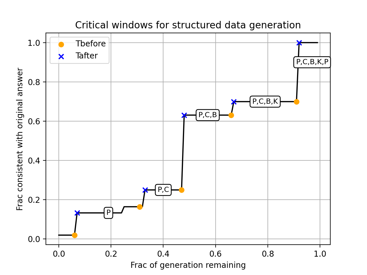
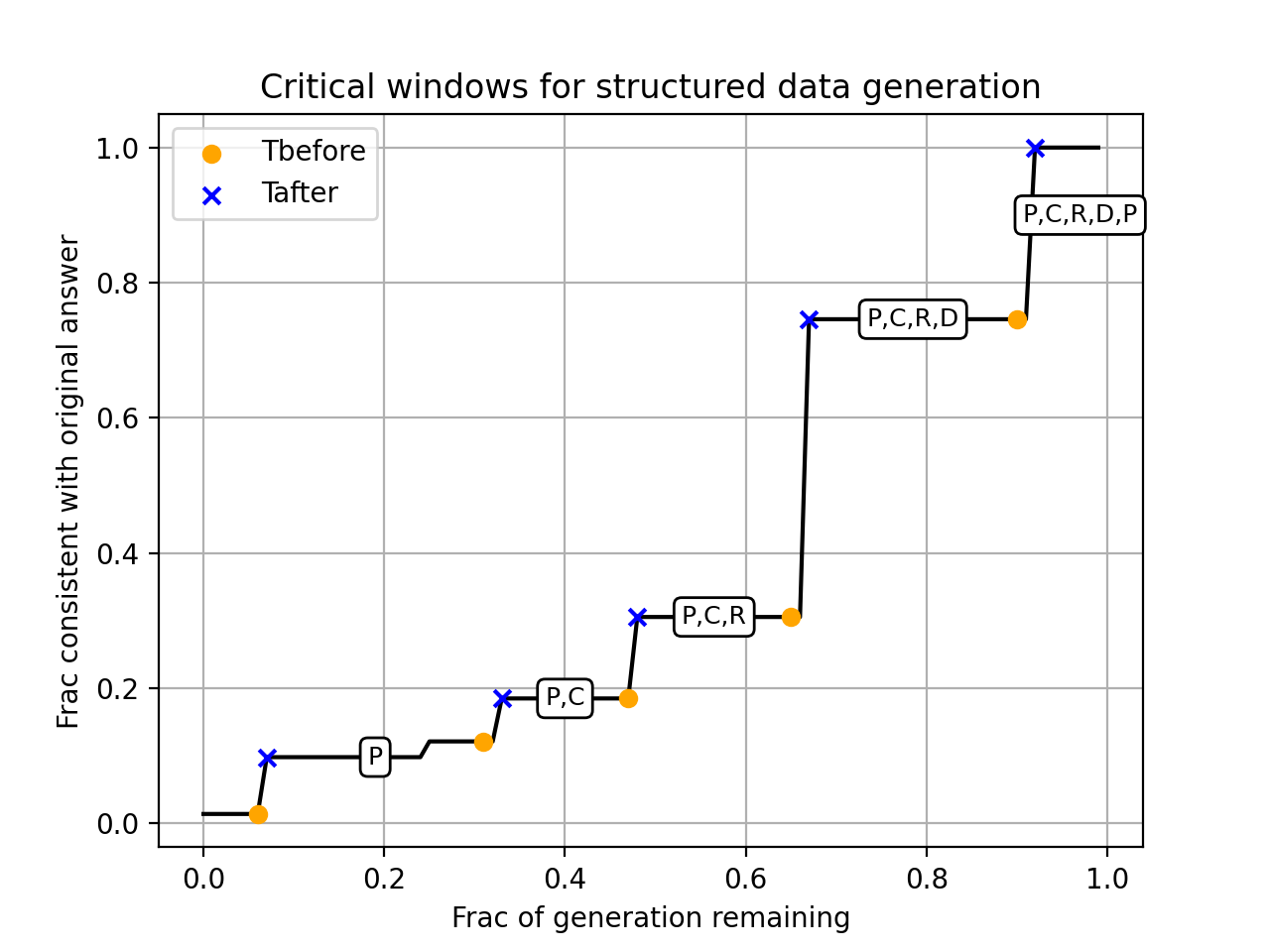
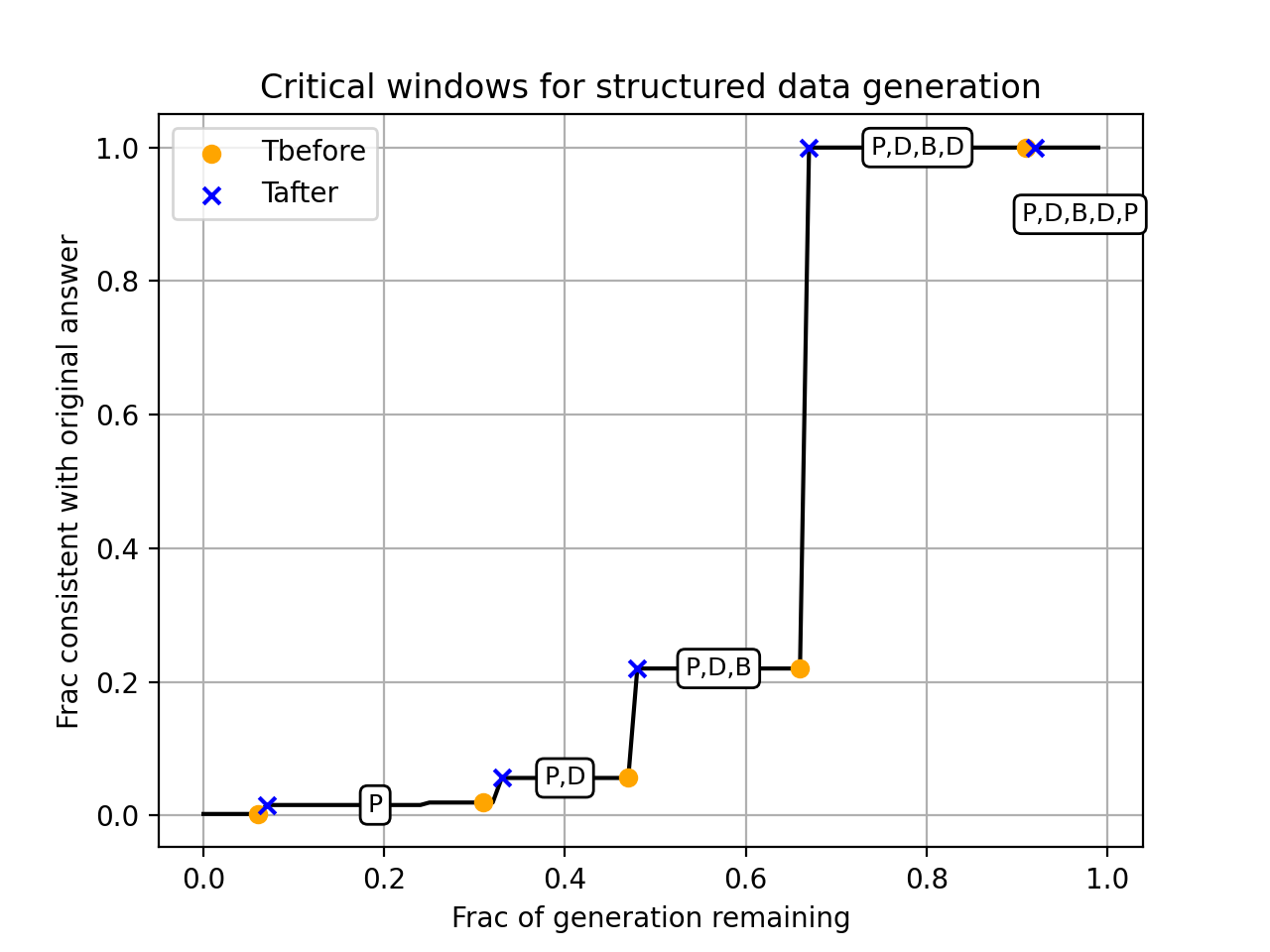
Figure 3: Structured output plots for LLAMA-$3.1$-$8$B-Instruct.

6.2 Chain of thought experiments

We then identify critical windows for LLAMA-$3.1$-$8$B-Instruct, Phi-$3$-$7$B-Instruct, and Qwen-$2.5$-$7$B-Instruct on $7$ different math and reasoning benchmarks on which performance is known to improve with chain of thought reasoning [38]: ARC Challenge and Easy [12], AQua [46], LogiQA [37], MMLU [31], and TruthfulQA [39] multiple-choice benchmarks and the MATH benchmark from [32]. In the forward-reverse experiments, we take the original generation, truncate a fraction of tokens, and check if resampling yields the same answer, using a direct text comparison for the multiple choice benchmarks and the prm800k grader for MATH [41]. We do this for $400$ questions from each dataset and resample at each truncation fraction $100$ times. Critical windows, defined as a $>0.5$ jump in probability of obtaining the same answer in consecutive truncation fractions, appear prominently across all models and benchmarks that we tested (Figures 4, 8, and 9); for MATH, they occur in $42.2\%,16.6\%,30.2\%$ of generations from LLAMA-$3.1$-$8$B-Instruct, Qwen-$2.5$-$7$B-Instruct, and Phi-$3$-$7$B-Instruct.

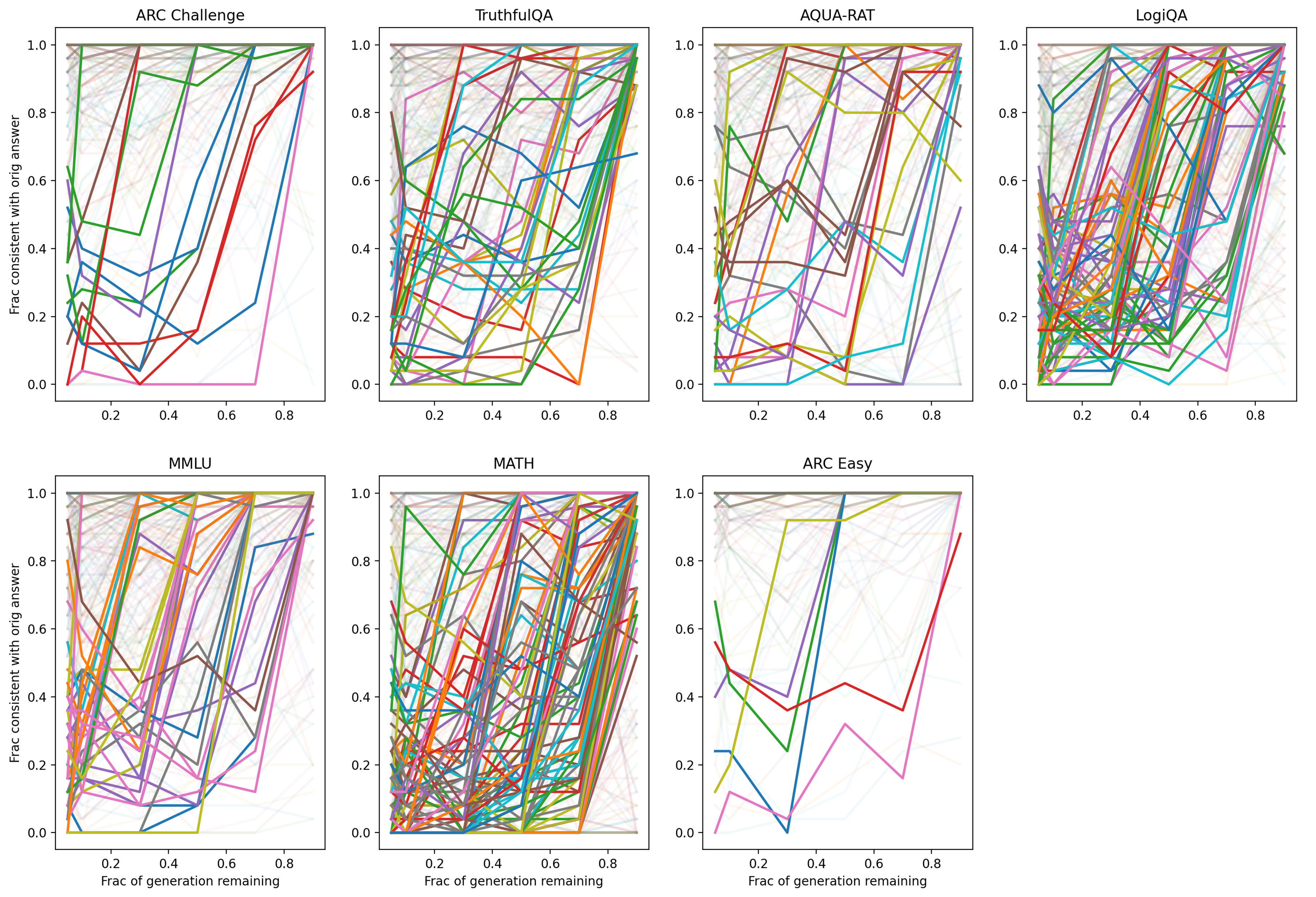
Figure 4: Probability that the answer is the same as a function of the percentage of the generation remaining for different math and reasoning benchmarks for LLAMA-$3.1$-$8$B-Instruct. Highlighted are generations with a 50% increase and no 30% decrease in the probability over one step.

These jumps occur during important steps of reasoning: in Figure 5, the correct formula is first expressed in the critical window. Furthermore, we find that generations with critical windows are significantly less accurate than generations without critical windows across all datasets and models. For LLAMA-$3.1$-$8$B-Instruct, critical windows result in up to 73% lower accuracy, and incorrect responses contain 11%-33% more critical windows (Table 1).

Table 1: Differences between Accuracy (Acc) without versus with critical windows and frequency of critical windows (CW) when the original generation is wrong versus right.

Dataset	LLAMA-$3.1$-$8$B-Instruct		Phi-$3$-$7$B-Instruct		Qwen-$2.5$-$7$B-Instruct
	$\Delta$Acc	$\Delta$CW	$\Delta$Acc	$\Delta$CW	$\Delta$Acc	$\Delta$CW
AQUA-RAT	0.42	0.20	0.36	0.16	0.03	0.01
ARC Challenge	0.53	0.22	0.50	0.24	0.38	0.11
ARC Easy	0.73	0.26	0.28	0.13	0.40	0.07
LogiQA	0.15	0.11	0.21	0.19	0.23	0.11
MATH	0.41	0.33	0.36	0.33	0.46	0.29
MMLU	0.45	0.24	0.38	0.21	0.26	0.11
TruthfulQA	0.44	0.20	0.42	0.23	0.55	0.23

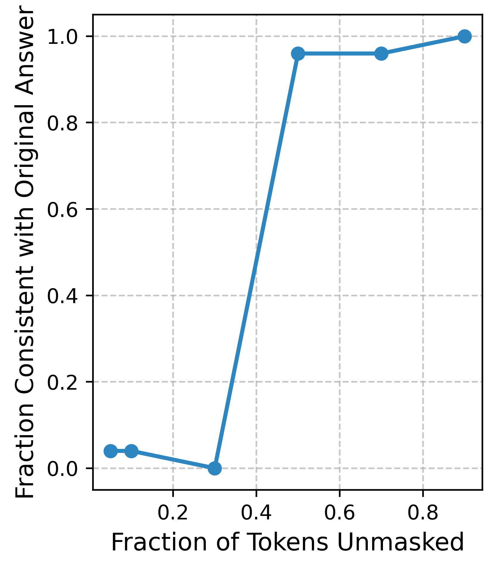
Figure 5: Example of critical window for Phi-$3$-$7$B-Instruct (bolded).

7 Discussion

In this work, we developed a simple yet general theory for critical windows for stochastic localization samplers like diffusion and autoregressive models. Already, practitioners have applied critical windows to make LLMs safer [56] and reason better [1, 42]. Our theory significantly streamlines our understanding of critical windows and provides concrete insights for practitioners. We pair our theory with extensive experiments, and demonstrate its usefulness in monitoring for jailbreaks and understanding reasoning failures.

Limitations.

The theory applies to the most prominent and empirically successful generative models (autoregressive language models, continuous diffusion and flow matching models). However, some less widely-used generative models do not belong to the family of localization-based samplers. Generative adversarial networks [24] and consistency models [62] both use a singular evaluation of a neural network to map noise into an image. However, we argue the restriction to the localization-based samplers is extremely minor because these models are either not widely used in practice or based on localization-based samplers.

Future Work.

While we instantiate our theory in many settings (Section 4), an important future direction is compute the location of critical windows in other settings and connect it to statistical physics predictions for other models of data, e.g., the random hierarchy model [63].

Impact statement.

Though this paper is largely theoretical in nature, it does describe a theory for jailbreaks which could impact model safety in the future. We hope the insights in this manuscript about jailbreaks lead to better alignment strategies and training methods.

Appendix A Additional related work

Theory of in-context learning for language models.

With respect to theory for language models, our results are most closely related to the Bayesian framework for in-context learning [71, 8, 26, 76, 3]. For example, [71] also considered a mixture model of topics and showed that language models can learn the underlying class despite in-context learning and training distribution mismatch. We view this manuscript as connecting the Bayesian framework for in-context learning to other empirical phenomena observed in language models and diffusion models and the all-or-nothing phenomenon.

Chain of thought.

[42, 1] also observed that the presence of critical windows in the chain of thought of math and reasoning tasks and their significance in leading the model to incorrect outputs, concurrent with our results in Figure 5. They then used them to provide rewards or data for a preference optimization algorithm to improve reasoning performance. [42] called them critical tokens and utilized a contrastive estimation algorithm to identify critical windows and provide token-level rewards. The Phi-4 Technical report called them pivotal tokens, developed a binary-search based algorithm to identify the location of critical windows, and used them to produce contrasting pairs for preference optimization [1]. Using our broad theoretical perspective, we provide new insight into critical windows of these kinds and view our work as corroborating and extending these empirical works.

Jailbreaks.

Existing work on jailbreaks has studied the appearance of critical windows in the first few generated tokens [56, 73, 35, 44]. Our theory provides a simple explanation for when jailbreaks occur: when the unaligned component assigns a much higher probability to the current text than the aligned component, then the model is jailbroken. This generalizes the explanation from [56] (see Example 4 for our particular formalism of their insights). It also explains the success of perplexity-based monitors for jailbreaks [4], which monitor for a low probability of the context and generation. We view our work as providing a rigorous mathematical framework for jailbreaks, as well as highlighting the important role off-distribution contexts play in eliciting harmful behaviors; we also develop a novel jailbreak from our framework (Section D.1.2 ) similar to the adversarial contrast decoding method proposed by [75], which also uses a likelihood ratio between an unaligned and an aligned model. However, we use a jailbroken and non-jailbroken pair of models instead of two versions of the model with different prompts.

Appendix B Examples of stochastic localization samplers

In this section, we present several kinds of generative models within the stochastic localization framework and their forward and reverse processes.

Example 8 (Continuous Diffusion Models [36]).

For continuous diffusion models, the forward process progressively degrades samples $X\sim p$ into pure Gaussian noise through scaling and convolution with Gaussian noise. It is the Ornstein-Uhlenbeck process, a stochastic process $(X_{t})_{t\geq 0}$ given by the following stochastic differential equation (SDE),

$$\mathrm{d}X_{t}=-X_{t}\,\mathrm{d}t+\sqrt{2}\mathrm{d}B_{t}\,,\qquad X_{0}\sim p\,,$$ (4)

where $(B_{t})_{t\geq 0}$ is a standard Brownian motion. Let $q_{t}\triangleq\mathrm{law}(X_{t})$ for $t\geq 0$, and observe that as $t\to\infty$, $q_{t}$ converges exponentially quickly to the standard Gaussian distribution $\mathcal{N}(0,\mathrm{Id})$. Assume we end the forward process at time $T\geq 0.$ For the reverse process $(X^{\scriptscriptstyle\leftarrow}_{t})_{t\in[0,T]}$, we employ the reversal of the Ornstein-Uhlenbeck SDE, given by

$$\mathrm{d}X^{\scriptscriptstyle\leftarrow}_{t}=\{X^{\scriptscriptstyle\leftarrow}_{t}+2\nabla\ln q_{T-t}(X^{\scriptscriptstyle\leftarrow}_{t})\}\,\mathrm{d}t+\sqrt{2}\,\mathrm{d}B_{t}\,,\qquad X^{\scriptscriptstyle\leftarrow}_{T}\sim q_{T}\,$$ (5)

where here $(B_{t})_{t\geq 0}$ is also a Brownian motion. Defining $(Y_{t})_{t\in\mathbf{I}}=(X_{t})_{t\in\mathbf{I}}$, we see that the forward process satisfies the Markov property in Definition 1, and the information from the original sample $X_{0}$ is degraded by more steps in the SDE. Furthermore, the reverse SDE with parameterized by the score function $\nabla\ln q_{T-t}(X^{\scriptscriptstyle\leftarrow}_{t})$ can be viewed as successively sampling from the posteriors via Tweedie’s formula.

Example 9 (Discrete Diffusion Models [43]).

Consider a set $\mathcal{A}$ denoting the vocabulary and let $p\in\mathcal{A}^{T}$, and consider a forward process with index set $\mathbf{I}=[0,K]\cup\{\infty\}$, $Y_{0}=X$, and $Y_{t}\in\mathcal{A}^{T}$ defined in the limit as follows,

$$p(Y_{t+\Delta t}=a\mid Y_{t}=b)=\delta_{ab}+Q_{t}(b,a)\Delta t+O(\Delta t^{2}),$$

where $Q_{t}\in\mathbb{R}^{n\times n}$ are diffusion matrices with nonnegative non-diagonal entries and columns which sum to $0$. $(Y_{t})_{t\in\mathbf{I}}$ is also a Markov chain and as $t\to\infty$, $Y_{t}$ is degraded until it is eventually uninformative about the original sample $Y_{0}$.

Example 10 (Autoregressive Language Models).

Consider a set $\mathcal{A}$ denoting the vocabulary and let $p\in\mathcal{A}^{T}$, and consider a forward process with index set $\mathbf{I}=\{0,1,2,\dots,T\}$, $Y_{0}=X$, and $Y_{t}\in\mathcal{A}^{T-t}$. For $t\in\mathbf{I}$, we let $Y_{t}$ equal the last first $T-t$ tokens of $X$. Clearly this is a Markov Chain, and the reverse process is equivalent to next-token prediction.

Appendix C Proof details

C.1 Deferred details from Section 3

For Theorem 2, we employ the following two helper lemmas.

See 3

Proof.

We can rewrite $P^{\scriptscriptstyle\leftarrow}(x|Y_{\widehat{T}}),P^{\scriptscriptstyle\leftarrow}(x|Y_{\widehat{T}},S_{\mathrm{target}})$ using the law of total probability and Bayes’ rule.

$$P^{\scriptscriptstyle\leftarrow}(x|Y_{\widehat{T}}) =\sum_{\theta\in\Theta}P^{\scriptscriptstyle\leftarrow}_{t\to\Theta}(\theta|Y_{\widehat{T}})P^{\scriptscriptstyle\leftarrow}(x|Y_{\widehat{T}},\theta)$$

$$P^{\scriptscriptstyle\leftarrow}(x|Y_{\widehat{T}},S_{\mathrm{target}}) =\sum_{\theta\in S_{\mathrm{target}}}P^{\scriptscriptstyle\leftarrow}_{t\to\Theta}(\theta|Y_{\widehat{T}},S_{\mathrm{target}})P^{\scriptscriptstyle\leftarrow}(x|Y_{\widehat{T}},\theta)=\frac{\sum_{\theta\in S_{\mathrm{target}}}P^{\scriptscriptstyle\leftarrow}_{t\to\Theta}(\theta|Y_{\widehat{T}})P^{\scriptscriptstyle\leftarrow}(x|Y_{\widehat{T}},\theta)}{\sum_{\theta\in S_{\mathrm{target}}}P^{\scriptscriptstyle\leftarrow}_{t\to\Theta}(\theta|Y_{\widehat{T}})}.$$

Note that the second equality on the second line follows from the fact that for all $\theta\in S_{\mathrm{target}}$, the posteriors $P^{\scriptscriptstyle\leftarrow}_{t\to\Theta}(\cdot|Y_{t})\propto P^{\scriptscriptstyle\leftarrow}_{t\to\Theta}(\cdot|Y_{t},S_{\mathrm{target}})$ by the same normalization constant. Therefore the difference can be written as

$$\int\left|P^{\scriptscriptstyle\leftarrow}(x|Y_{\widehat{T}})-P^{\scriptscriptstyle\leftarrow}(x|Y_{\widehat{T}},S_{\mathrm{target}})\right|dx$$

$$=\int\left|\sum_{\theta\in\Theta}P^{\scriptscriptstyle\leftarrow}_{t\to\Theta}(\theta|Y_{\widehat{T}})P^{\scriptscriptstyle\leftarrow}(x|Y_{\widehat{T}},\theta)-\frac{\sum_{\theta\in S_{\mathrm{target}}}P^{\scriptscriptstyle\leftarrow}_{t\to\Theta}(\theta|Y_{\widehat{T}})P^{\scriptscriptstyle\leftarrow}(x|Y_{\widehat{T}},\theta)}{\sum_{\theta\in S_{\mathrm{target}}}P^{\scriptscriptstyle\leftarrow}_{t\to\Theta}(\theta|Y_{\widehat{T}})}\right|dx$$

$$=\int\Bigg{|}\left(1-\frac{1}{\sum_{\theta\in S_{\mathrm{target}}}P^{\scriptscriptstyle\leftarrow}_{t\to\Theta}(\theta|Y_{\widehat{T}})}\right)\sum_{\theta\in S_{\mathrm{target}}}P^{\scriptscriptstyle\leftarrow}_{t\to\Theta}(\theta|Y_{\widehat{T}})P^{\scriptscriptstyle\leftarrow}(x|Y_{\widehat{T}},\theta)+\sum_{\theta\in\Theta-S_{\mathrm{target}}}P^{\scriptscriptstyle\leftarrow}_{t\to\Theta}(\theta|Y_{\widehat{T}})P^{\scriptscriptstyle\leftarrow}(x|Y_{\widehat{T}},\theta)\Bigg{|}dx.$$

If $\sum_{\theta\in\Theta-S_{\mathrm{target}}}P^{\scriptscriptstyle\leftarrow}_{t\to\Theta}(\theta|Y_{\widehat{T}})=0$, then the above is equal to $0$ and we are done. If it is non-zero, we can factor out $\sum_{\theta\in\Theta-S_{\mathrm{target}}}P^{\scriptscriptstyle\leftarrow}_{t\to\Theta}(\theta|Y_{\widehat{T}})$ term, which allows us to write everything in terms of posteriors with respect to $\Theta-S_{\mathrm{target}}$ and $S_{\mathrm{target}}$,

$$\int\Bigg{|}\left(1-\frac{1}{\sum_{\theta\in S_{\mathrm{target}}}P^{\scriptscriptstyle\leftarrow}_{t\to\Theta}(\theta|Y_{\widehat{T}})}\right)\sum_{\theta\in S_{\mathrm{target}}}P^{\scriptscriptstyle\leftarrow}_{t\to\Theta}(\theta|Y_{\widehat{T}})P^{\scriptscriptstyle\leftarrow}(x|Y_{\widehat{T}},\theta)+\sum_{\theta\in\Theta-S_{\mathrm{target}}}P^{\scriptscriptstyle\leftarrow}_{t\to\Theta}(\theta|Y_{\widehat{T}})P^{\scriptscriptstyle\leftarrow}(x|Y_{\widehat{T}},\theta)\Bigg{|}dx$$

$$=\sum_{\theta\in\Theta-S_{\mathrm{target}}}P^{\scriptscriptstyle\leftarrow}_{t\to\Theta}(\theta|Y_{\widehat{T}})\int\left|P^{\scriptscriptstyle\leftarrow}(x|Y_{\widehat{T}},S_{\mathrm{target}})-P^{\scriptscriptstyle\leftarrow}(x|Y_{\widehat{T}},\Theta-S_{\mathrm{target}})\right|dx$$

Employing the trivial observation that

$$\int\left|P^{\scriptscriptstyle\leftarrow}(x|Y_{\widehat{T}},S_{\mathrm{target}})-P^{\scriptscriptstyle\leftarrow}(x|Y_{\widehat{T}},\Theta-S_{\mathrm{target}})\right|dx$$

$$\leq\int P^{\scriptscriptstyle\leftarrow}(x|Y_{\widehat{T}},S_{\mathrm{target}})+P^{\scriptscriptstyle\leftarrow}(x|Y_{\widehat{T}},\Theta-S_{\mathrm{target}})dx\leq 2,$$

we have

$$\int\left|P^{\scriptscriptstyle\leftarrow}(x|Y_{\widehat{T}})-P^{\scriptscriptstyle\leftarrow}(x|Y_{\widehat{T}},S_{\mathrm{target}})\right|dx\leq 2\sum_{\theta\in\Theta-S_{\mathrm{target}}}P^{\scriptscriptstyle\leftarrow}_{t\to\Theta}(\theta|Y_{\widehat{T}}).$$

∎

See 4

Proof.

We obtain through Bayes’ rule,

$$\sum_{\theta\in\Theta-S_{\mathrm{target}}}P^{\scriptscriptstyle\leftarrow}_{t\to\Theta}(\theta|Y_{\widehat{T}})=\frac{\sum_{\theta\in\Theta-S_{\mathrm{target}}}w_{\theta}p^{\theta}_{\widehat{T}}(Y_{\widehat{T}})}{\sum_{\theta\in\Theta}w_{\theta}p^{\theta}_{\widehat{T}}(Y_{\widehat{T}})}.$$

We divide by the same normalizing constant $\sum_{\theta\in\Theta-S_{\mathrm{target}}}w_{\theta}$ to obtain

$$\frac{\sum_{\theta\in\Theta-S_{\mathrm{target}}}w_{\theta}p^{\theta}_{\widehat{T}}(Y_{\widehat{T}})}{\sum_{\theta\in\Theta}w_{\theta}p^{\theta}_{\widehat{T}}(Y_{\widehat{T}})} =\frac{\frac{\sum_{\theta\in\Theta-S_{\mathrm{target}}}w_{\theta}p^{\theta}_{\widehat{T}}(Y_{\widehat{T}})}{\sum_{\theta\in\Theta-S_{\mathrm{target}}}w_{\theta}}}{\frac{\sum_{\theta\in\Theta-S_{\mathrm{target}}}w_{\theta}p^{\theta}_{\widehat{T}}(Y_{\widehat{T}})}{\sum_{\theta\in\Theta-S_{\mathrm{target}}}w_{\theta}}+\frac{\sum_{\theta\in S_{\mathrm{target}}}w_{\theta}p^{\theta}_{\widehat{T}}(Y_{\widehat{T}})}{\sum_{\theta\in S_{\mathrm{target}}}w_{\theta}}\cdot\frac{\sum_{\theta\in S_{\mathrm{target}}}w_{\theta}}{\sum_{\theta\in\Theta-S_{\mathrm{target}}}w_{\theta}}}$$

$$\leq\max\left(1,\frac{\sum_{\theta\in\Theta-S_{\mathrm{target}}}w_{\theta}}{\sum_{\theta\in S_{\mathrm{target}}}w_{\theta}}\right)\frac{p^{\Theta-S_{\mathrm{target}}}_{\widehat{T}}(Y_{\widehat{T}})}{p^{\Theta-S_{\mathrm{target}}}_{\widehat{T}}(Y_{\widehat{T}})+p^{S_{\mathrm{target}}}_{\widehat{T}}(Y_{\widehat{T}})}.$$

∎

C.2 Proofs for Section 4

C.2.1 Diffusions

Here we use an alternative $f$-divergence to characterize the critical windows, the squared Hellinger distance, defined as $\mathrm{H}^{2}(P,Q)\triangleq\int(\sqrt{dP}-\sqrt{dQ})^{2}d\mu$, because there are explicit computations for the Hellinger distance for mixtures of Gaussians. We similarly exploit the following ratio inequality akin to Lemma 1,

Lemma 7.

For probability measures $P,Q$,

$$\mathbb{E}_{x\sim P}\left[\frac{\mathrm{d}Q}{\mathrm{d}P+\mathrm{d}Q}\right]\leq\frac{1}{2}(1-\frac{1}{2}\mathrm{H}^{2}(P,Q)).$$

We apply the following well-known formula for the Hellinger distance between two Gaussians.

Lemma 8.

We have

$$1-\frac{1}{2}H^{2}(\mathcal{N}(\mu_{P},\Sigma_{P}),\mathcal{N}(\mu_{Q},\Sigma_{Q}))=\frac{|\Sigma_{P}|^{1/4}|\Sigma_{Q}|^{1/4}}{\left|\frac{\Sigma_{P}+\Sigma_{Q}}{2}\right|^{1/2}}\exp\left\{-\frac{1}{8}(\mu_{P}-\mu_{Q})^{\top}\left[\frac{\Sigma_{P}+\Sigma_{Q}}{2}\right]^{-1}(\mu_{P}-\mu_{Q})\right\}.$$

See 1

Proof.

The proof for $T_{\mathrm{before}}$, a simple application of Pinsker’s inequality, can be found in Appendix B.1 of [36]. Directly applying the new Master Theorem 2 to $T_{\mathrm{after}}$, we need only show that

$$\frac{\sqrt{2}}{2}\left(1-\frac{1}{2}\mathrm{H}^{2}(p^{+1}_{T_{\mathrm{after}}},p^{-1}_{T_{\mathrm{after}}})\right)\leq\frac{\sqrt{2}}{2}\exp(-\frac{1}{2}\|\mu\|^{2}e^{-2t})\leq\epsilon.$$

∎

See 2

Proof.

The proof for $T_{\mathrm{before}}$ can be found in Section 5.2 of [36]. We need to slightly modify the proof of Theorem 2 so that we can write the desired bound for $T_{\mathrm{after}}$ in terms of the Hellinger distance of individual components. We use the same notation. By convexity, we can bound

$$\mathbb{E}_{Y_{\widehat{T}}\sim p^{S_{\mathrm{target}}}_{\widehat{T}}}\left[\frac{\sum_{\theta\in\Theta-S_{\mathrm{target}}}w_{\theta}p^{\theta}_{\widehat{T}}(Y_{\widehat{T}})}{\sum_{\theta\in\Theta}w_{\theta}p^{\theta}_{\widehat{T}}(Y_{\widehat{T}})}\right] \leq\sum_{\theta\in\Theta-S_{\mathrm{target}}}w_{\theta}\sum_{\phi\in S_{\mathrm{target}}}w_{\phi}\mathbb{E}_{Y_{\widehat{T}}\sim p^{\phi}_{\widehat{T}}}\left[\frac{p^{\theta}_{\widehat{T}}(Y_{\widehat{T}})}{w_{\theta}p^{\theta}_{\widehat{T}}(Y_{\widehat{T}})+w_{\phi}p^{\phi}_{\widehat{T}}(Y_{\widehat{T}})}\right]$$

$$\leq K\max_{\theta\in\Theta-S_{\mathrm{target}},\phi\in S_{\mathrm{target}}}\left(1-\frac{1}{2}\mathrm{H}^{2}(p^{\theta}_{\widehat{T}},p^{\phi}_{\widehat{T}})\right)\leq\epsilon,$$

when $\widehat{T}\leq T_{\mathrm{after}}$. To conclude the second part of the theorem, observe that by concentration of measure (e.g., Theorem 3.1.1 from [68]) and a union bound, there exists a constant $T$ independent of $d$ such that $\|\mu_{j}\|\in[\sqrt{d}-T,\sqrt{d}+T]$ for all $j\in[K]$ with high probability. Furthermore, by known Gaussian Suprema inequalities, we can also assume that there exists a constant $T^{\prime}$ independent of $d$ such that $|\langle\mu_{i},\mu_{j}\rangle|\leq T^{\prime}\|\mu_{i}\|$ (Lemma 5.1 from [69]). Thus, we can conclude that

$$\max_{j\in[K]}\|\mu_{i}-\mu_{j}\|^{2} \leq 2d+4T\sqrt{d}+2T^{2}+2T^{\prime}(\sqrt{d}+T)=O(d).$$

$$\max_{j\in[K]}\|\mu_{i}-\mu_{j}\|^{2} \geq 2d-4T\sqrt{d}+2T^{2}-2T^{\prime}(\sqrt{d}+T)=\Omega(d).$$

The difference in $\log$ scale is thus constant,

$$\frac{1}{2}\left(\ln\max_{j\in[K]}\|\mu_{i}-\mu_{j}\|^{2}-\ln\min_{j\in[K],i\neq j}\|\mu_{i}-\mu_{j}\|^{2}\right)=O_{K,\epsilon}(1)$$

∎

See 3

Proof.

To prove $\mathrm{TV}(p^{1,\widehat{T}},p^{1})\lesssim\epsilon$ when $\widehat{T}\leq T_{\mathrm{after}}$, observe that when $\widehat{T}\leq T_{\mathrm{after}}$, the probability that all the differing elements between $\ell_{1},\ell_{-1}$ are masked is exactly $\widehat{T}^{d_{H}(\delta_{\ell_{1}},\delta_{\ell_{-1}})}\leq\epsilon^{2}$. That means that there exists a set $A$ with $p^{+1}_{\widehat{T}}(A)\geq 1-\epsilon^{2}$ and $p^{-1}_{\widehat{T}}(A)=0$, so by the definition of total variation, $\mathrm{TV}(p^{+1}_{\widehat{T}},p^{-1}_{\widehat{T}})\geq 1-\epsilon^{2}$. Obviously, $\mathrm{TV}(p^{+1}_{\widehat{T}},p^{+1}_{\widehat{T}})=0$ as well, so by Theorem 2, we obtain $\mathrm{TV}(p^{1,\widehat{T}},p^{1})\lesssim\epsilon$. To prove that $\mathrm{TV}(p^{1,\widehat{T}},p^{\{\pm 1\}})\leq\epsilon$ when $\widehat{T}\geq T_{\mathrm{before}}$, we need only show that $\mathrm{TV}(p^{+1}_{\widehat{T}},p_{\widehat{T}})\leq\epsilon$. By Lemma 15 of [36], it suffices to show that $\mathrm{TV}(p^{+1}_{\widehat{T}},p^{-1}_{\widehat{T}})\leq\epsilon$ by a simple triangle inequality argument. Consider the set $A\subset\{\pm 1,\mathrm{[MASKED]}\}^{T}$ such that $\mathrm{TV}(p^{+1}_{\widehat{T}},p^{-1}_{\widehat{T}})=p^{+1}_{\widehat{T}}(A)-p^{-1}_{\widehat{T}}(A)$. Consider the set $B=\mathrm{supp}(p^{+1}_{\widehat{T}})\cap\mathrm{supp}(p^{-1}_{\widehat{T}})$. For any $x\in B$, we know $p^{+1}_{\widehat{T}}(x)=p^{-1}_{\widehat{T}}(x)$ because the same number of tokens need to be masked from $\ell_{\pm 1}$. This means we have $p^{+1}_{\widehat{T}}(B)=p^{-1}_{\widehat{T}}(B)\geq\widehat{T}^{d_{H}(\ell_{+1},\ell_{-1})}\geq 1-\epsilon$. Because $p^{+1}_{\widehat{T}}(A)-p^{-1}_{\widehat{T}}(A)=p^{+1}_{\widehat{T}}(A-B)-p^{-1}_{\widehat{T}}(A-B)$, we have $p^{+1}_{\widehat{T}}(A)-p^{-1}_{\widehat{T}}(A)\leq p^{+1}_{\widehat{T}}(\{\pm 1,\mathrm{[MASKED]}\}^{T}-B)\leq\epsilon$. ∎

C.2.2 Autoregression

See 5

Proof.

Because only the direction of steps matter, we can model the critical window for this random walk as observing a sequence of $\pm 1$ with an autoregressive language model. Let $p\in\{\pm 1\}^{T}$, and consider a forward process with index set $\mathbf{I}=\{0,1,2,\dots,T\}$, $Y_{0}=X$, and $Y_{t}\in\{\pm 1,\mathrm{[MASKED]}\}^{T}$. For $t\in\mathbf{I}$, we let the last $t$ tokens of $Y_{t}$ be deterministically set to $\mathrm{[MASKED]}$. We generate data as a mixture of biased coins with separation $2\Delta<0.01.$ For a mixture of two biased coins, with probabilities of $0.5\pm\Delta$ ($\theta_{\pm 1}$ respectively) of yielding $1$, we can compute the critical window and show that it tightly clusters around $\Theta(1/\Delta^{2})$. Let $\Theta=\{\theta_{\pm 1}\},p^{\theta_{\pm 1}}\sim(\textrm{Bern}(\theta_{\pm 1}))^{\otimes T},w_{\pm 1}=\frac{1}{2}$. We also assume $\epsilon^{2}<10^{-3}(0.5-\Delta)(0.5+\Delta)$. Then, on component $1$ we have the critical window $T_{\mathrm{before}}=T-\frac{\epsilon^{2}}{\Delta^{2}}+2$ and $T_{\mathrm{after}}=T-\frac{\ln(2/\epsilon^{2})}{2\Delta^{2}}.$ When $\widehat{T}\leq T_{\mathrm{after}}$, then $\mathrm{TV}(p^{1,\widehat{T}},p^{1})\lesssim\epsilon$. When $\widehat{T}\geq T_{\mathrm{before}}$, $\mathrm{TV}(p^{1,\widehat{T}},p)\lesssim\epsilon$.

Note that the number of $+1$ is sufficient for disambiguating $\theta_{\pm 1}$. To prove the bounds $T_{\mathrm{before}}$, we show that with only $\frac{\epsilon^{2}}{\Delta^{2}}-2$ samples the total variation between $0.5-\Delta$ and $0.5+\Delta$ is negligible. Using [59], we find

$$\mathrm{TV}(p^{+1}_{T_{\mathrm{after}}},p^{-1}_{T_{\mathrm{after}}})\leq\frac{2\Delta\sqrt{\frac{T-T_{\mathrm{after}}+2}{2(0.5-\Delta)(0.5+\Delta)}}}{\left(1-2\Delta\sqrt{\frac{T-T_{\mathrm{after}}+2}{2(0.5-\Delta)(0.5+\Delta)}}\right)^{2}}\lesssim 3\epsilon.$$

For $T_{\mathrm{after}}$, we compute how many samples it takes for $p^{\pm 1}$ to have only $\epsilon$ overlap in total variation using Hoeffding’s inequality. If we have $n$ samples, the mean $\overline{X}$ of the $n$ samples of $\pm 1$ for $p=0.5+\Delta$ satisfies the concentration inequality $P(|\overline{X}-2\Delta|>\Delta)\leq 2\exp(-2nt^{2})$ (furthermore we can ignore the stopping condition by our requirement that $\frac{\ln(2/\epsilon^{2})}{2\Delta^{2}}<A$). We find $P(|\overline{X}-2\Delta|>\Delta)\leq\epsilon^{2}$ for $T-T_{\mathrm{after}}$ samples, proving that the total variation is at least $1-\epsilon^{2}$. ∎

C.2.3 Autoregressive model with a Gaussian mixture model as the underlying concept distribution

We consider a model for autoregressive data similar to the one presented in [5]. Each word is a vector $w\in\mathbb{R}^{d}$ and the context length is $T\in\mathbb{Z}^{>0}$. The original samples are $x\in\mathbb{R}^{T\times d}$. Let $\Theta=\{u,v\}$, where $u,v\in\mathcal{S}^{d-1}$. We define the distribution $p^{\theta}$ for $\theta\in\Theta$ as follows. We generate the path of a discourse vector $\left(C_{t}^{\theta}\right)_{t\in[0,\infty]}\in\mathbb{R}^{d}$ with the reverse SDE Orstein-Uhlenbeck process such that $C_{\infty}^{\theta}\sim\mathcal{N}(0,\mathrm{Id})$ and $C_{0}^{\theta}\sim\mathcal{N}(0,\mathrm{Id}+\alpha\theta\theta^{\top})$ for some $\alpha>0$. We let $q^{\theta}_{t}$ be the law of $C^{\theta}_{t}$ for $t\geq 0$. We let $\mathbf{I}=\{0,1,\dots,T\}$, and for $t\in\mathbf{I}$, we draw samples $w^{\theta}_{t}\in\mathbb{R}^{d}$ where we impose a normal Gaussian prior and have $w^{\theta}_{t}|C_{t}^{\theta}\propto\exp(\langle C_{t}^{\theta},\cdot\rangle)$. Then we return the corpus $\{w^{\theta}_{t}\}_{t\in\mathbf{I}}$ as an output.

Theorem 9 (Autoregressive with a mixture of two Gaussians as the concept distribution ).

We assume that $\exp(-T)\sqrt{\alpha-\log(1+\alpha)}\leq\epsilon$. Let $\phi(x)=\frac{2+x}{(2+x(1+\langle u,v\rangle)/2)(2+x(1-\langle u,v\rangle)/2)}$. Then, on component $u$ we have

$$T_{\mathrm{after}}=\frac{1}{2}\ln\left[\frac{\alpha}{\phi^{-1}(\epsilon^{2})}\right],T_{\mathrm{before}}=\frac{1}{2}\ln\left[\frac{\alpha\sqrt{1+\alpha^{2}}\sqrt{1-\langle u,v\rangle^{2}}}{\epsilon}\right].$$ (5)

When $\widehat{T}\leq T_{\mathrm{after}}$, then $\mathrm{TV}(p^{\{u\},\widehat{T}},p^{\{u\}})\lesssim\epsilon$. When $\widehat{T}\geq T_{\mathrm{before}}$, $\mathrm{TV}(p^{\{u\},\widehat{T}},p)\lesssim\epsilon$.

This proof will require Theorem 10 and Lemmas 8 and 11, which is stated below:

Theorem 10 (Section 5.2 of [13]).

Let $(Y_{t})_{t\in[0,T]}$ and $(Y^{\prime}_{t})_{t\in[0,T]}$ denote the solutions to

$$\mathrm{d}Y_{t} =b_{t}(Y_{t})\,\mathrm{d}t+\sqrt{2}\mathrm{d}B_{t}\,,\qquad Y_{0}\sim q$$

$$\mathrm{d}Y^{\prime}_{t} =b^{\prime}_{t}(Y^{\prime}_{t})\,\mathrm{d}t+\sqrt{2}\mathrm{d}B_{t}\,,\qquad Y^{\prime}_{0}\sim q\,.$$

Let $q$ and $q^{\prime}$ denote the laws of $Y_{T}$ and $Y^{\prime}_{T}$ respectively. If $b_{t},b^{\prime}_{t}$ satisfy that $\int^{T}_{0}\mathbb{E}_{Q}\,\|b_{t}(Y_{t})-b^{\prime}_{t}(Y_{t})\|^{2}\,\mathrm{d}t<\infty$, then $\mathrm{KL}(q\|q^{\prime})\leq\int^{T}_{0}\mathbb{E}_{Q}\,\|b_{t}(Y_{t})-b^{\prime}_{t}(Y_{t})\|^{2}\,\mathrm{d}t$.

Lemma 11.

Let $u,v\in\mathcal{S}^{d-1}$. Then

$$\|uu^{\top}-vv^{\top}\|_{\rm op} \leq\sqrt{1-\langle u,v\rangle^{2}}$$

$$\lambda(uu^{\top}+vv^{\top}) =\{1\pm\langle u,v\rangle\}.$$

Proof.

There exists $r\in\mathcal{S}^{d-1}$ such that $v=\langle u,v\rangle u+\sqrt{1-\langle u,v\rangle^{2}}r$ and $u\perp r$. We find that

$$uu^{\top}-vv^{\top}=(1-\langle u,v\rangle^{2})uu^{\top}-(1-\langle u,v\rangle^{2})rr^{\top}-\langle u,v\rangle\sqrt{1-\langle u,v\rangle^{2}}[ur^{\top}+ru^{\top}].$$

We can explicitly compute the eigenvalues of $uu^{\top}-vv^{\top}$ using the discriminant and find that they are equal to $\pm\sqrt{1-\langle u,v\rangle^{2}}.$ By a similar derivation, we can write

$$uu^{\top}+vv^{\top}=(1+\langle u,v\rangle^{2})uu^{\top}+(1-\langle u,v\rangle^{2})rr^{\top}+\langle u,v\rangle\sqrt{1-\langle u,v\rangle^{2}}[ur^{\top}+ru^{\top}].$$

which gives us eigenvalues for $uu^{\top}+vv^{\top}$ of $1\pm\langle u,v\rangle$. ∎

Proof.

To compute the $T_{\mathrm{after}}$ bounds, we compare the difference in Hellinger distance of the distribution of words words at generated at index $\widehat{T}$, $w^{u}_{\widehat{T}}$. By the data processing inequality $1-\frac{1}{2}H^{2}(p^{u}_{\widehat{T}},p^{v}_{\widehat{T}})\leq 1-\frac{1}{2}H^{2}(w^{u}_{\widehat{T}},w^{v}_{\widehat{T}})$, so it suffices to show $1-\frac{1}{2}H^{2}(w^{u}_{\widehat{T}},w^{v}_{\widehat{T}})\lesssim\epsilon$. Because the Gaussian is its own conjugate prior and $w^{u}_{\widehat{T}}|C^{\theta}_{t}\propto\exp(-\frac{1}{2}\|w^{u}_{\widehat{T}}-C^{\theta}_{t}\|^{2})$, we can compute $w^{u}_{\widehat{T}}|C^{\theta}_{t}\sim\mathcal{N}(C^{\theta}_{t},\mathrm{Id})$ and $w^{u}_{\widehat{T}}\sim\mathcal{N}(0,2\mathrm{Id}+\alpha e^{-2t}uu^{\top})$. Applying Lemmas 8 and 11, we can explicitly compute

$$1-\frac{1}{2}H^{2}(w^{u}_{\widehat{T}},w^{v}_{\widehat{T}})\lesssim\sqrt{\frac{2+\alpha e^{-2\widehat{T}}}{(2+\alpha e^{-2\widehat{T}}(1+\langle u,v\rangle)/2)(2+\alpha e^{-2\widehat{T}}(1-\langle u,v\rangle)/2)}}\lesssim\sqrt{\phi(\alpha e^{-2\widehat{T}})}\leq\epsilon.$$

To compute $T_{\mathrm{before}}$, we first use the data processing inequality to reduce the difference in the emitted tokens to the difference in the paths of the context vectors, and then apply the approximation error bounds from Theorem 10 to bound the differences in path measures. When $\widehat{T}\geq T_{\mathrm{before}}$, we can use the triangle inequality to write $\mathrm{TV}(p^{\{u\},\widehat{T}},p)=\mathrm{TV}(p^{u}_{\widehat{T}},p^{\{u,v\}}_{\widehat{T}})\leq\mathrm{TV}(p^{u}_{\widehat{T}},p^{v}_{\widehat{T}})$. Note that $p^{\theta}_{\widehat{T}}$ is the distribution of the first $T-\widehat{T}$ tokens generated by the model under $\theta$. Note that $p^{u}_{\widehat{T}}$ is a function of $(C^{u}_{t})_{t\in\mathbf{I}\cap[\widehat{T},T]}$ and $p^{v}_{\widehat{T}}$ is a function of $(C^{v}_{t})_{t\in\mathbf{I}\cap[\widehat{T},T]}$. By the data processing inequality, we can bound the difference in terms of the distributions over the tokens in terms of the law of the process of the discourse vectors,

$$\mathrm{TV}(p^{u}_{\widehat{T}},p^{v}_{\widehat{T}})\leq\mathrm{TV}((C^{u}_{t})_{t\in\mathbf{I}\cap[\widehat{T}]},(C^{v}_{t})_{t\in\mathbf{I}\cap[\widehat{T},T]})\leq\mathrm{TV}((C^{u}_{t})_{t\in[\widehat{T},T]},(C^{v}_{t})_{t\in[\widehat{T},T]}).$$

Note that for $\theta\in\Theta$, $(C^{\theta}_{t})_{t\in[\widehat{T},T]}$ is generated by the following reverse time SDE,

$$\mathrm{d}C^{\theta}_{t}=\{C^{\theta}_{t}+2\nabla\ln q^{\theta}_{t}(C^{\theta}_{t})\}\,\mathrm{d}t+\sqrt{2}\,\mathrm{d}B_{t},\qquad t\in[\widehat{T},T],C^{\theta}_{T}\sim q^{\theta}_{T}.$$ (6)

Now we define $(C^{u\to v}_{t})_{t\in[\widehat{T},T]}$ to be the reverse SDE defined by initializing at $q^{u}_{T}$ but with the score of $q^{v}_{t}$,

$$\mathrm{d}C^{u\to v}_{t}=\{C^{u\to v}_{t}+2\nabla\ln q^{v}_{t}(C^{u\to v}_{t})\}\,\mathrm{d}t+\sqrt{2}\,\mathrm{d}B_{t},\qquad t\in[\widehat{T},T],C^{u\to v}_{T}\sim q^{u}_{T}.$$ (7)

By the triangle inequality, we have

$$\mathrm{TV}((C^{u}_{t})_{t\in[\widehat{T},T]},(C^{v}_{t})_{t\in[\widehat{T},T]})\leq\underbrace{\mathrm{TV}((C^{u}_{t})_{t\in[\widehat{T},T]},(C^{u\to v}_{t})_{t\in[\widehat{T},T]})}_{\text{(I)}}+\underbrace{\mathrm{TV}((C^{u\to v}_{t})_{t\in[\widehat{T},T]},(C^{v}_{t})_{t\in[\widehat{T},T]})}_{\text{(II)}}.$$

To bound (I), observe that the SDEs have different scores but the same initializations. We apply Theorem 10 to $\mathrm{TV}((C^{u}_{t})_{t\in[\widehat{T},T]},(C^{u\to v}_{t})_{t\in[\widehat{T},T]})$ and obtain

$$\mathrm{TV}((C^{u}_{t})_{t\in[\widehat{T},T]},(C^{u\to v}_{t})_{t\in[\widehat{T},T]}) \leq\sqrt{\mathrm{KL}((C^{u}_{t})_{t\in[\widehat{T},T]}||(C^{u\to v}_{t})_{t\in[\widehat{T},T]})}$$

$$\leq\sqrt{\int_{\widehat{T}}^{T}\mathbb{E}_{X\sim C^{u}_{t}}\|\nabla\ln p^{u}_{t}(X)-\nabla\ln p^{v}_{t}(X)\|^{2}dt}$$

We simplify the inner expectation by using the

$$\|\nabla\ln p^{u}_{t}(X)-\nabla\ln p^{v}_{t}(X)\| =\|\left[(\mathrm{Id}+\alpha e^{-2t}uu^{\top})^{-1}-(\mathrm{Id}+\alpha e^{-2t}vv^{\top})^{-1}\right]x\|$$

$$=\|\left[\left(\mathrm{Id}-\frac{\alpha e^{-2t}}{1+\alpha e^{-2t}}uu^{\top}\right)-\left(\mathrm{Id}-\frac{\alpha e^{-2t}}{1+\alpha e^{-2t}}vv^{\top}\right)\right]x\|$$

$$\lesssim\alpha e^{-2t}\|uu^{\top}-vv^{\top}\|_{\rm op}\left\|\prod_{\textrm{span}(u,v)}x\right\|,$$

$$=\alpha e^{-2t}\sqrt{1-\langle u,v\rangle^{2}}\left\|\prod_{\textrm{span}(u,v)}x\right\|.\quad(\text{Lemma}~\ref{lem:opnormtwovec})$$

We can upper bound $\mathbb{E}_{X\sim C^{u}_{t}}\|\prod_{\textrm{span}(u,v)}X\|^{2}$ by considering right-triangular $L$ such that $L^{\top}L=\mathrm{Id}+\alpha uu^{\top}$. and $\prod_{\textrm{span}(u,v)}X=\prod_{\textrm{span}(u,v)}LY$, where $Y\sim\mathcal{N}(0,\mathrm{Id})$. The operator norm of $\prod_{\textrm{span}(u,v)}L$ is

$$\left\|\prod_{\textrm{span}(u,v)}\circ L\right\|_{\rm op}\leq\left\|L\right\|_{\rm op}\leq\sqrt{1+\alpha^{2}e^{-2t}}\leq\sqrt{1+\alpha^{2}}.$$

$\prod_{\textrm{span}(u,v)}\circ L$ is also rank $2$ and $\left(\prod_{\textrm{span}(u,v)}\circ L\right)Y=\left(\prod_{\textrm{span}(u,v)}\circ L\right)\circ\prod_{L^{-1}\textrm{span}(u,v)}Y$, where $\prod_{L^{-1}\textrm{span}(u,v)}Y\sim\mathcal{N}(0,\mathrm{Id}_{2})$. Thus we have

$$\mathbb{E}_{Y\sim\mathcal{N}(0,\mathrm{Id})}\left[\left\|\left(\prod_{\textrm{span}(u,v)}\circ L\right)Y\right\|^{2}\right]=\mathbb{E}_{Y^{\prime}\sim\mathcal{N}(0,\mathrm{Id}_{2})}\left[\left\|\left(\prod_{\textrm{span}(u,v)}\circ L\right)Y^{\prime}\right\|^{2}\right]\lesssim 1+\alpha^{2}$$

Combining this information together, we are able to compute,

$$\mathrm{TV}((C^{u}_{t})_{t\in[\widehat{T},T]},(C^{u\to v}_{t})_{t\in[\widehat{T},T]}) \leq\sqrt{\int_{\widehat{T}}^{T}\mathbb{E}_{X\sim C^{u}_{t}}\|\nabla\ln p^{u}_{t}(X)-\nabla\ln p^{v}_{t}(X)\|^{2}dt}$$

$$\lesssim\alpha\sqrt{1+\alpha^{2}}\sqrt{1-\langle u,v\rangle^{2}}e^{-2\widehat{T}}$$

$$\lesssim\epsilon.$$

To bound (II), we observe that both are run with the same score so we need only bound the difference at initialization. By the data processing inequality, we again have $\mathrm{TV}((C^{u\to v}_{t})_{t\in[\widehat{T},T]},(C^{v}_{t})_{t\in[\widehat{T},T]})\leq\mathrm{TV}(p^{u}_{T},p^{v}_{T})$. We can again apply the triangle inequality to get $\mathrm{TV}(p^{u}_{T},p^{v}_{T})\leq\mathrm{TV}(p^{u}_{T},\gamma^{d})+\mathrm{TV}(\gamma^{d},p^{v}_{T})\leq$. For any $\theta\in\Theta$, we have by the forward convergence of the OU process $\mathrm{TV}(p^{u}_{T},\gamma^{d})\leq\exp(-T)\sqrt{\mathrm{KL}(p_{u}||\gamma^{d})}$. We can explicitly compute $\mathrm{KL}(p_{u}||\gamma^{d})$ as

$$\mathrm{KL}(p_{u}||\gamma^{d})=\frac{1}{2}\left[d+\alpha-d-\log(\mathrm{Id}+\alpha uu^{\top})\right]=\frac{1}{2}\left[\alpha-\log(1+\alpha)\right].$$

Thus, we obtain the following bound on $\mathrm{TV}((C^{u\to v}_{t})_{t\in[\widehat{T},T]},(C^{v}_{t})_{t\in[\widehat{T},T]})$ of

$$\mathrm{TV}((C^{u\to v}_{t})_{t\in[\widehat{T},T]},(C^{v}_{t})_{t\in[\widehat{T},T]}) \lesssim\exp(-T)\sqrt{\alpha-\log(1+\alpha)}\lesssim\epsilon.\qed$$

C.2.4 Interweaving transitions from other distributions

In this section, we extend our critical windows framework to the setting where at certain steps of sampling procedure, instead of using the reverse Markov transition kernel from the original stochastic localization sampler, we use an alternative distribution which is not necessarily related to the original sampler. This includes many important applications of generative models, in which one seeks to combine the priors learned from data with some other algorithm. For example, one may want to combine the language model with a problem generation oracle in in-context learning [19].

As [71] points out, the transition from the answer to one problem to the problem statement of another example in-context learning is determined by an alternative transition kernel (which they call $p_{\textrm{prompt}}$). Although the probability of transition from one answer to the problem statement of another example is extremely low under the natural data distribution, one still hopes that with sufficiently many samples, the model selects the correct $\theta^{*}\in\Theta$ if these lower probability transitions are overcome by the distributional difference for $\theta\in\Theta$ with $\theta\neq\theta^{*}$. Similarly, under our critical windows framework, we can hope to capture the idea that we specialize to a particular $\theta^{*}$ given a sufficiently long context. In Section C.2.5, we first present a general framework for characterizing critical windows in this setting. Then, in section C.2.6, we consider the case of in-context learning by autoregressive language models and prove convergence.

C.2.5 General interweaving framework

We present this framework for the case where the index set $\mathbf{I}=\{0,1,\dots,m\}$ is discrete. Like before, assume we have a series of reverse Markov transition kernels $P^{\scriptscriptstyle\leftarrow,p}_{k\to k-1}(\cdot|\cdot)$, for $k\in\mathbf{I}$, but we also assume we have an alternative distribution $P^{\scriptscriptstyle\leftarrow,\mathrm{alt}}_{k\to k-1}(\cdot|\cdot)$ that we use to sample for transitions $k\in A\subsetneq\mathbf{I}$. For our sampling procedure, we sample $Y_{m}$, and for $k=m-1,m-2,\dots,0$, we take $Y_{k}\sim P^{\scriptscriptstyle\leftarrow,p}_{k+1\to k}(\cdot|Y_{k+1})$ for $k\in\mathbf{I}-A$ and $Y_{k}\sim P^{\scriptscriptstyle\leftarrow,\mathrm{alt}}_{k+1\to k}(\cdot|Y_{k+1})$ for $k\in A$. We denote the final distribution $p^{\mathrm{alt}}$.

Now, we also need to adjust our definitions of $p^{S}$ to this particular sampling procedure. We define $p^{S,\mathrm{alt}}$ for $S\subset\Theta$ to the distribution over outputs when we instead use the kernels $P^{\scriptscriptstyle\leftarrow}_{k+1\to k}(\cdot|Y_{k+1},S)$ instead of $P^{\scriptscriptstyle\leftarrow}_{k+1\to k}(\cdot|Y_{k+1})$. To relate $p^{\theta,\mathrm{alt}}$ to $p^{\theta,\mathrm{alt}}$ for $\theta\in\Theta$, we need to assume transitions from $\mathrm{alt}$ do not affect the posterior distribution over $p^{\Theta}(\theta|Y_{t})$.

Assumption 1.

For all $y\in\mathbb{R}$ and $x\in\mathrm{supp}(P^{\scriptscriptstyle\leftarrow,\mathrm{alt}}_{k+1\to k}(\cdot|y))$, we have for all $\theta,\theta^{\prime}\in\Theta$, the equality $P^{\scriptscriptstyle\leftarrow}_{k+1\to k}(x|y,\theta)=P^{\scriptscriptstyle\leftarrow}_{k+1\to k}(x|y,\theta^{\prime})$.

Adopting our definitions from Section 3, we let

$$T_{\mathrm{lower},\mathrm{alt}}(\epsilon)\in\{ t\in\mathbf{I}:\mathrm{TV}(p_{t}^{S_{\mathrm{init}},\mathrm{alt}},p_{t}^{S_{\mathrm{target}},\mathrm{alt}})\leq\epsilon\}$$ (8)

$$T_{\mathrm{upper},\mathrm{alt}}(\epsilon)\in\{ t\in\mathbf{I}:\mathrm{TV}(p_{t}^{S_{\mathrm{target}},\mathrm{alt}},p_{t}^{\Theta-S_{\mathrm{target}},\mathrm{alt}})\geq 1-\epsilon^{2}\,\}.$$ (9)

The main challenge of the below corollary is simply show that the final distribution $p^{\Theta,\mathrm{alt}}$ can be written as a mixture of $p^{\theta,\mathrm{alt}}$ with the same mixing weights as before.

Corollary 3.

Under Assumption 1, for $\epsilon>0$, if $\widehat{T}\geq T_{\mathrm{lower},\mathrm{alt}}(\epsilon)$ and $\widehat{T}\leq T_{\mathrm{upper},\mathrm{alt}}(\epsilon)$, then

$$\mathrm{TV}(p^{S_{\mathrm{init}},\widehat{T}},p^{S_{\mathrm{target}},\mathrm{alt}})\leq\left(1+\sqrt{2}\max\left(1,\frac{\sum_{\theta\in\Theta-S_{\mathrm{target}}}w_{\theta}}{\sum_{\theta\in S_{\mathrm{target}}}w_{\theta}}\right)/2\right)\epsilon.$$ (10)

Proof.

We need only show that $p^{\Theta,\mathrm{alt}}\triangleq\sum_{\theta\in\Theta}w_{\theta}p^{\theta,\mathrm{alt}}$. It suffices to shows that the probability of generating a path $Y_{m},Y_{m-1},\dots,Y_{0}$ are the same under both density functions. We need only consider transitions for $k\in\mathbf{I}-A$, because for $k\in A$, the transitions are both given by the alternative distribution. For the transitions not given by $\mathrm{alt}$, note that we are using the original model, so

$$p^{\Theta,\mathrm{alt}}(Y_{k-1}|Y_{k})=\frac{\sum_{\theta\in\Theta}w_{\theta}p^{\theta}(Y_{k})P^{\scriptscriptstyle\leftarrow}_{k\to k-1}(Y_{k-1}|Y_{k},\theta)}{\sum_{\theta\in\Theta}w_{\theta}p^{\theta}(Y_{k})}.$$ (11)

Furthermore, for the mixture model, this probability is

$$p^{\mathrm{mix}}=\frac{\sum_{\theta\in\Theta}w_{\theta}p^{\theta,\mathrm{alt}}(Y_{m},Y_{m-1},\dots,Y_{k+1},Y_{k})P^{\scriptscriptstyle\leftarrow}_{k\to k-1}(Y_{k-1}|Y_{k},\theta)}{\sum_{\theta\in\Theta}w_{\theta}p^{\theta,\mathrm{alt}}(Y_{m},Y_{m-1},\dots,Y_{k+1},Y_{k})}.$$ (12)

The distinction between Equation 11 and Equation 12 is that in the former we are using the likelihood of $p^{\theta}$ instead of $p^{\theta,\mathrm{alt}}$. Thus it suffices to show that $p^{\theta}\propto p^{\theta,\mathrm{alt}}$. We explicitly write out the probability,

$$p^{\theta}(Y_{m},Y_{m-1},\dots,Y_{k+1},Y_{k})=\prod_{i=k+1}^{m}p^{\theta}(Y_{i-1}|Y_{i})\propto\prod_{i=k+1,i\notin A}^{m}p^{\theta}(Y_{i-1}|Y_{i}),$$

where the proportionality follows from the fact that we can ignore the probability of the transitions produced by $\mathrm{alt}$ under Assumption 1. By definition, this is proportional to $p^{\theta,\mathrm{alt}}(Y_{m},Y_{m-1},\dots,Y_{k+1},Y_{k})$ up to a normalization constant independent of $\theta$. ∎

C.2.6 In-context learning

Now, we will specialize our framework to the case of in-context learning. As in [71], we assume that the language model is given inputs of the form $[x_{1},y_{1},o,x_{2},y_{2},o,\dots,x_{t},y_{t},o,x_{t+1}]$, where $x_{1}$ is the input, $y_{1}$ is the output, and $o$ is a delimiter token that separate different in-context samples from each other. We assume that the transitions $y_{i}\to o\to x_{i+1}$ are sampled by some alternative probability distribution $P_{\textrm{other}}(\cdot|\cdot)$. We require that $P_{\textrm{other}}$ selects the $x_{i}$ i.i.d.

Assumption 2.

The distribution of $P_{\textrm{other}}(x_{t+1}|x_{1},y_{1},o,x_{2},y_{2},o,\dots,x_{t},y_{t},o)=P_{\textrm{other}}(x_{1})$.

Then we assume that the transitions $x_{i}\to y_{i}$ are generated by some $\theta^{*}\in\Theta$, which does not depend on any of the previous tokens before the delimiter.

Assumption 3.

(Well-specification) There exists some $\theta^{*}\in\Theta$ such that $y_{i}$ is generated from $y_{i}\sim P^{\leftarrow}(\cdot|[x_{1},y_{1},o_{1},\dots,o_{i-1},x_{i}],\theta^{*})$.

Assumption 4.

For all $\theta\in\Theta$, we have $P^{\leftarrow}(\cdot|[x_{1},y_{1},o_{1},\dots,o_{i-1},x_{i}],\theta)=P^{\leftarrow}(\cdot|x_{i},\theta)$.

We also assume statistical separation of $\theta^{*}$ from $\Theta-\{\theta^{*}\}$ in terms of Hellinger distance.

Assumption 5.

Let $p_{(x,y)}^{S}$ for $S\subset\Theta$ be the distribution of $(x_{1},y_{1},o)$ where $x_{1}\sim P_{\textrm{other}}(\cdot|o)$ and $y_{1}\sim p^{S}(\cdot|x_{1})$. There exists $\delta>0$ such that $H^{2}(p_{(x,y)}^{\Theta-\{\theta^{*}\}},p_{(x,y)}^{\theta^{*}})\geq\delta.$

Example 11.

Let $T\geq\ln\left(\frac{1-\delta/2}{\epsilon}\right)$. Under Assumptions 1, 2, 3, 4, and 5, we have

$$\mathrm{TV}([x_{1},\dots,x_{T+1},y_{T+1}],[x_{1},\dots,x_{T+1},\tilde{y}_{T+1}])\lesssim\epsilon/w_{\theta^{*}}.$$

Proof.

It suffices to upper bound $1-\frac{1}{2}H^{2}(P^{\theta,\mathrm{alt}}_{3T},P^{\Theta-\{\theta\},\mathrm{alt}}_{3T})$ by $O(\epsilon)$. First observe that the distribution $p^{S,\mathrm{alt}}$ for $S\subset\Theta$ factors along the delimiters by a factor independent of $S$ using Assumptions 2 and  4, so we have

$$P^{S,\mathrm{alt}}_{3t}(x_{1},y_{1},o_{1},x_{2},y_{2},o_{2},\dots,x_{t},y_{t},o_{t})\propto\prod_{i=1}^{t}P^{S,\mathrm{alt}}_{3}(x_{i},y_{i},o_{i}).$$

Using the tensorization property of Hellinger distance and our definition of $T,\delta$, we have

$$1-\frac{1}{2}H^{2}(P^{\theta,\mathrm{alt}}_{3T},P^{\Theta-\{\theta\},\mathrm{alt}}_{3T}) \lesssim\left[1-\frac{1}{2}H^{2}(P^{\theta,\mathrm{alt}}_{3},P^{\Theta-\{\theta\},\mathrm{alt}}_{3})\right]^{T}\leq\epsilon.\qed$$

Appendix D Experiments

D.1 Jailbreak Experiments

D.1.1 Reproducing critical windows for jailbreaks from existing papers

Existing work has already identified the presence of critical windows in the domain of jailbreaks. Here we present critical windows for a simplified prefill jailbreak based on the prefill attack [30] and repeating token jailbreak [52] for LLAMA-$3.1$-$8$B-Instruct. In the first figure, we plot the probability of the model giving a harmful response, computed using the StrongReject Gemma 7b auditor from [65], as a function of the fraction of the phrase Sure, here is how to appended to the front of the model’s generation. We can see that there is a large jump in the attack success rate after only including a few tokens in the prefix. The second figure is a reproduction of Figure 12 from [52]. It shows that the probability of repeating the next token increases substantially as the first few tokens are included a few times in the context.

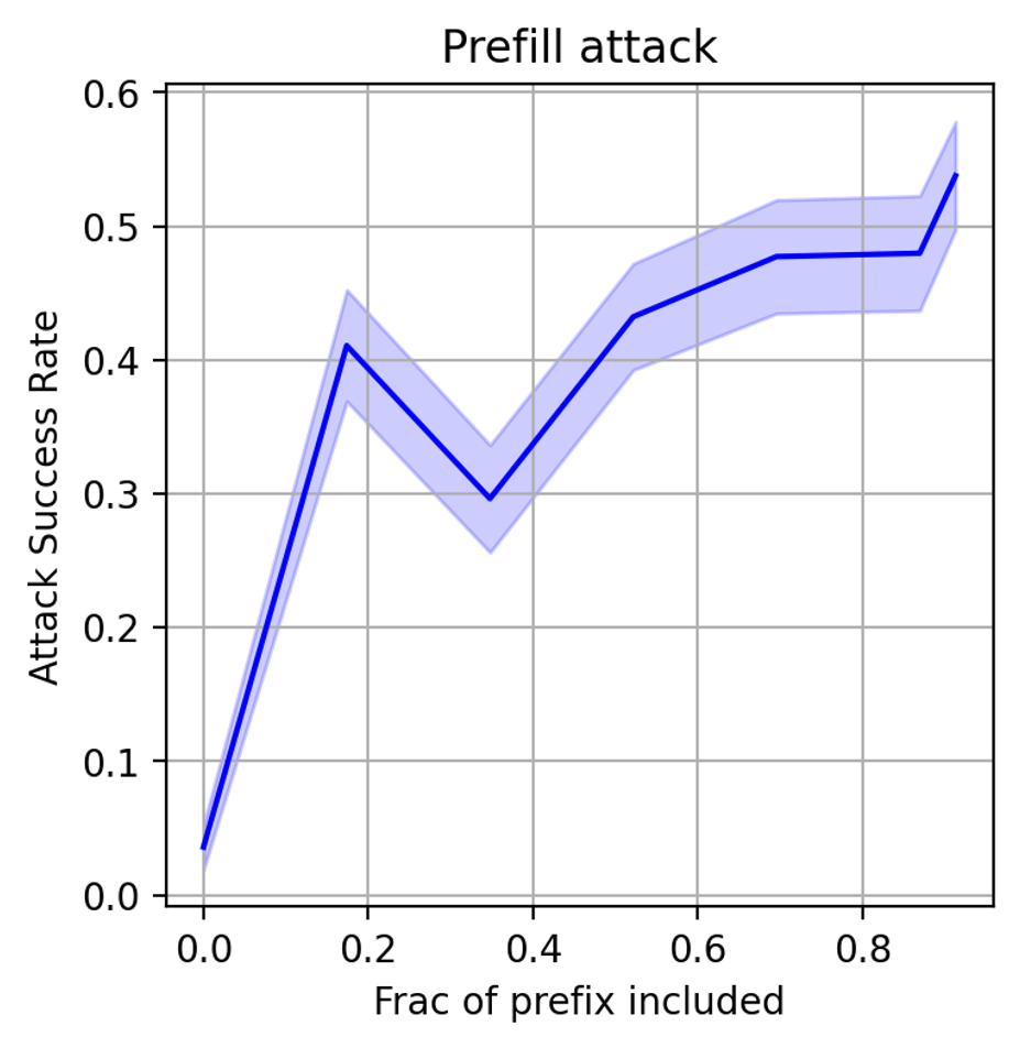
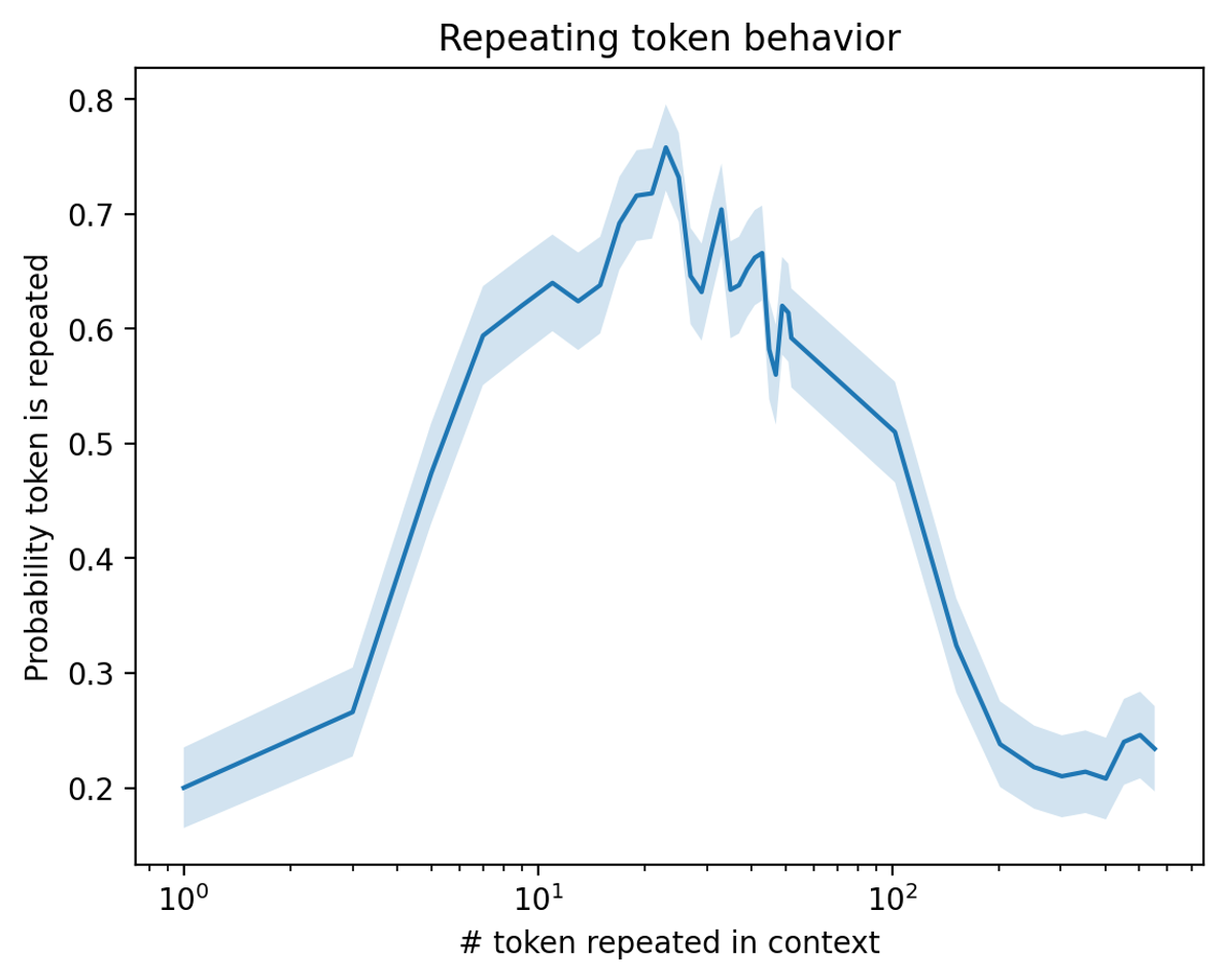
Figure 6: Examples of critical windows in jailbreaks for  LLAMA-$3.1$-$8$B-Instruct. Left: Critical window for a prefill jailbreak [30]. Right: Critical window for a repeating token jailbreak [52].

D.1.2 Experimental details from jailbreak

Now we apply our theory to develop a new jailbreak detection method, based on a likelihood ratio between an aligned and unaligned model. Intuitively, our theory states that when the unaligned component assigns a high probability to the text compared to the entire model, the model is likely to be jailbroken. We use a LLAMA-$3.1$-$8$B-Instruct model jailbroken with LoRA to not refuse harmful prompts [25] as a proxy for the unaligned model. We evaluate these different methods on a dataset of jailbreaks and benign prompts from [11].

Dataset.

We use the same dataset as [11] but provide details here for completeness. The benign dataset consists of inputs from UltraChat [18], a large dialogue dataset, and Xstest [58], which contains benign queries that are often incorrectly refused by language models. The benign queries are filtered to ensure that LLAMA-$3.1$-$8$B-Instruct does not refuse any of them. The dataset of harmful prompts is based off of the Circuit Breakers dataset [72]. The datasets include the following jailbreaking methods from the extant literature: PAIR [17], AutoDAN [45], Many-Shot Jailbreaking (MSJ) [2], Multi-Turn Attacks [40, 29], Prefill, GCG [74], and other Misc. attakcs from [70]. For each jailbreaking method, it is applied to a prompt from the Circuit Breaker dataset and evaluated to see if the generation from LLAMA-$3.1$-$8$B-Instruct is helpful and harmful, as determined by the StrongReject jailbreaking classifier [65]).

Evaluation Metric.

As is standard in the jailbreak detection literature [11], we report the recall at the false positive rate at $0.01$.

Table 2 displays the recall and several other baselines. Crucially, the log likelihood ratio methods does obtain recall $>1$ for $5$ different categories of jailbreaks. While our methods do perform worse than existing methods, it is important to note that they still work and that their poor performance could be explained by the fact that we have to use a proxy for the unaligned mode of the model.

Table 2: Recall (FPR=0.01) for our likelihood ratio threshold, a perplexity threshold  [4], and a MLP-based detector trained on activations [11] for predicting different jailbreaks. prompt/gen denote the logprobs of the prompt and generation, respectively.

	AutoDAN	GCG	Multi-Turn	Misc	MSJ	Pair	Prefill
$\log p^{\textrm{unaligned}}_{\textrm{prompt}}-\log p^{\textrm{aligned}}_{\textrm{prompt}}$	0.000	0.000	0.028	0.000	0.063	0.000	0.077
$\log p^{\textrm{unaligned}}_{\textrm{gen}}-\log p^{\textrm{aligned}}_{\textrm{gen}}$	0.082	0.030	0.000	0.100	0.000	0.061	0.051
$\log p^{\textrm{aligned}}_{\textrm{prompt}}$	0.000	0.576	0.056	0.063	0.013	0.000	0.077
$\log p^{\textrm{aligned}}_{\textrm{gen}}$	0.205	0.150	0.570	0.200	0.006	0.015	0.416
MLP	1.00	0.956	0.873	0.663	1.00	0.833	1.00

D.2 Chain of thought experiments

D.2.1 Experimental details

We describe the prompts we used in our evaluation of different datasets. The system prompt for all datasets is Produce a correct solution to the following /TASK/ question., where /TASK/ is the type of question of the dataset, i.e. science, math, or logic. For each question, we create a user prompt by appending Think of the /TASK/ question thoroughly step by step. Please only respond with the answer after reasoning thoroughly. in front of the question. Once the model completes its generation (max generation length set to $2048$ and default sampling parameters), we append the user prompt Given all of the above, what’s the single, most likely answer? Your answer should have the format "The answer is ANSWER", where ANSWER is your answer. for the multiple choice benchmarks and Given all of the above, what’s the single, most likely answer? Simplify it completely. Your answer should have the format "The answer is $ANSWER$", where ANSWER is your answer in LaTeX. Note that when we ask the model for the final answer, we set the temperature to $0$.

Across three different models ( LLAMA-$3.1$-$8$B-Instruct, Phi-$3$-$7$B-Instruct, and Qwen-$2.5$-$7$B-Instruct), we find that conditioned on the occurrence of critical windows, the model generation is significantly less accurate compared to generations without critical windows.

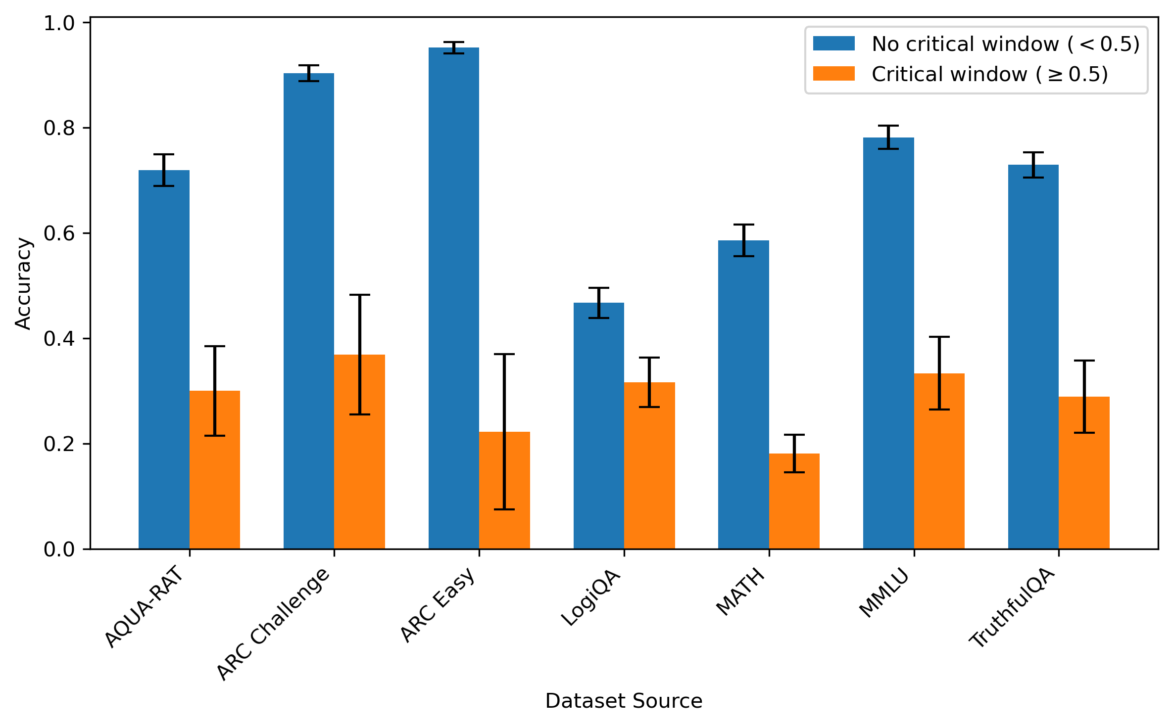
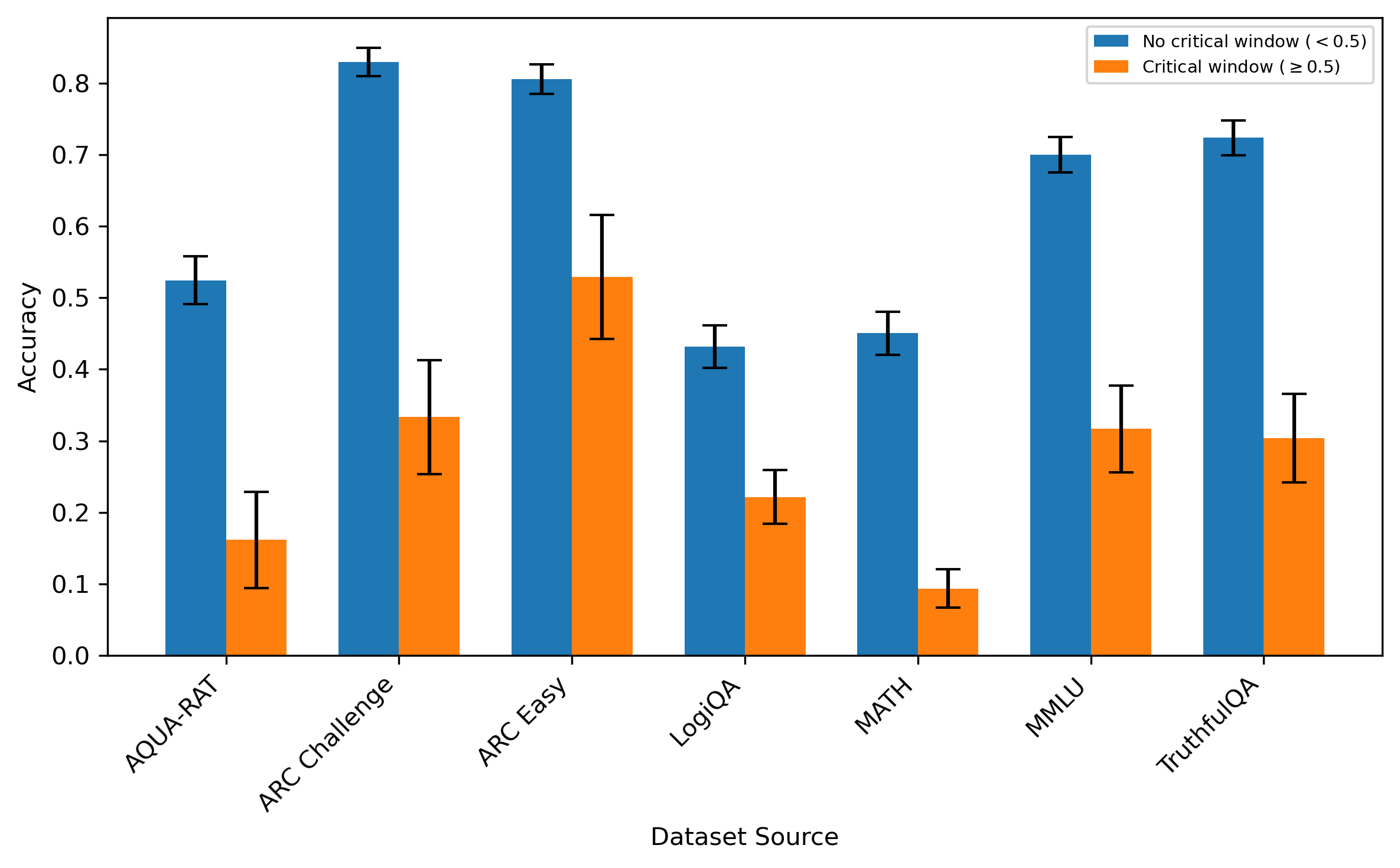
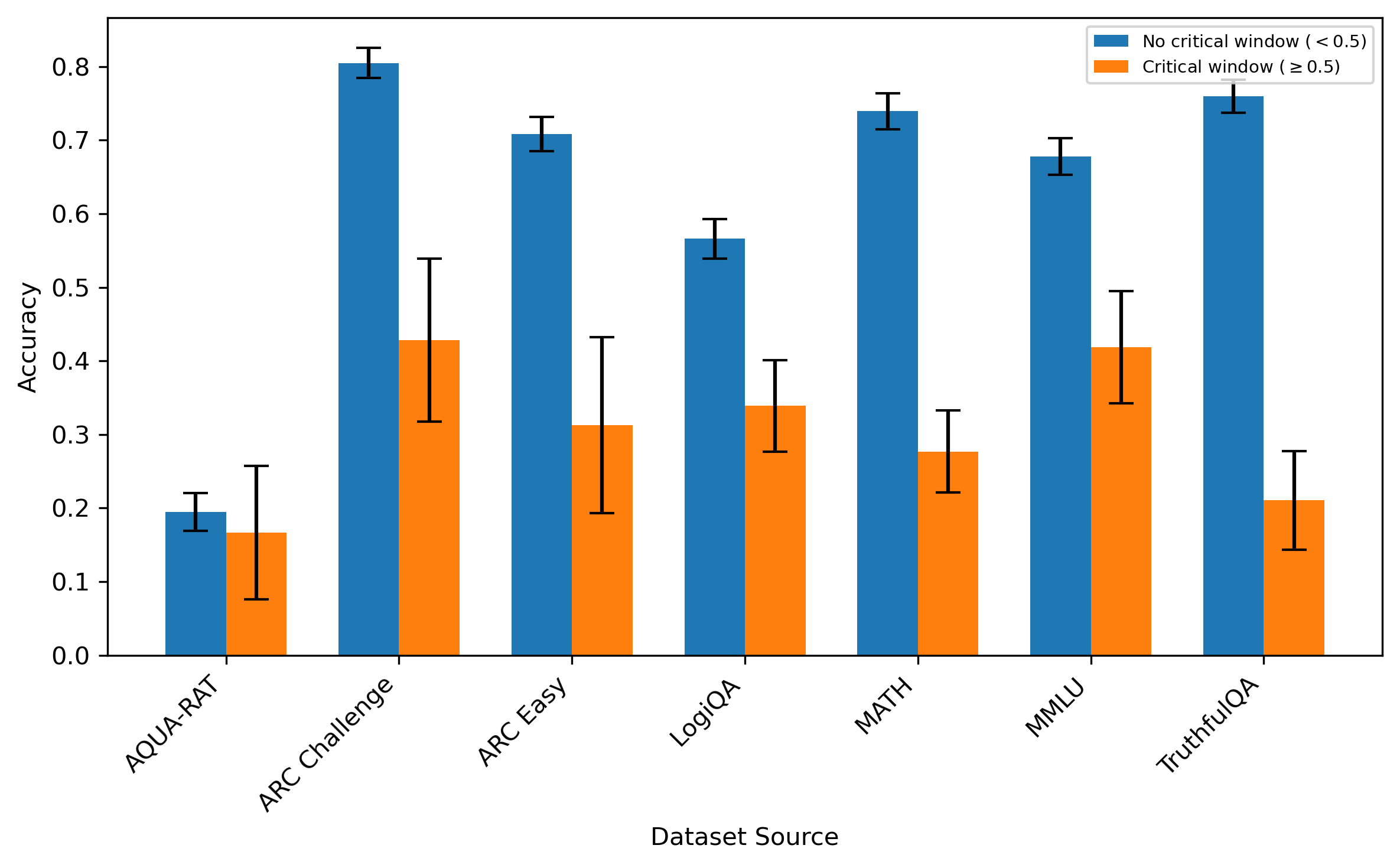
Figure 7: Left-to-right: LLAMA-$3.1$-$8$B-Instruct, Phi-$3$-$7$B-Instruct, and Qwen-$2.5$-$7$B-Instruct barplots of original generation accuracy for generations with ($\geq 0.5$ jump in probability) and without critical windows $(<0.5)$.

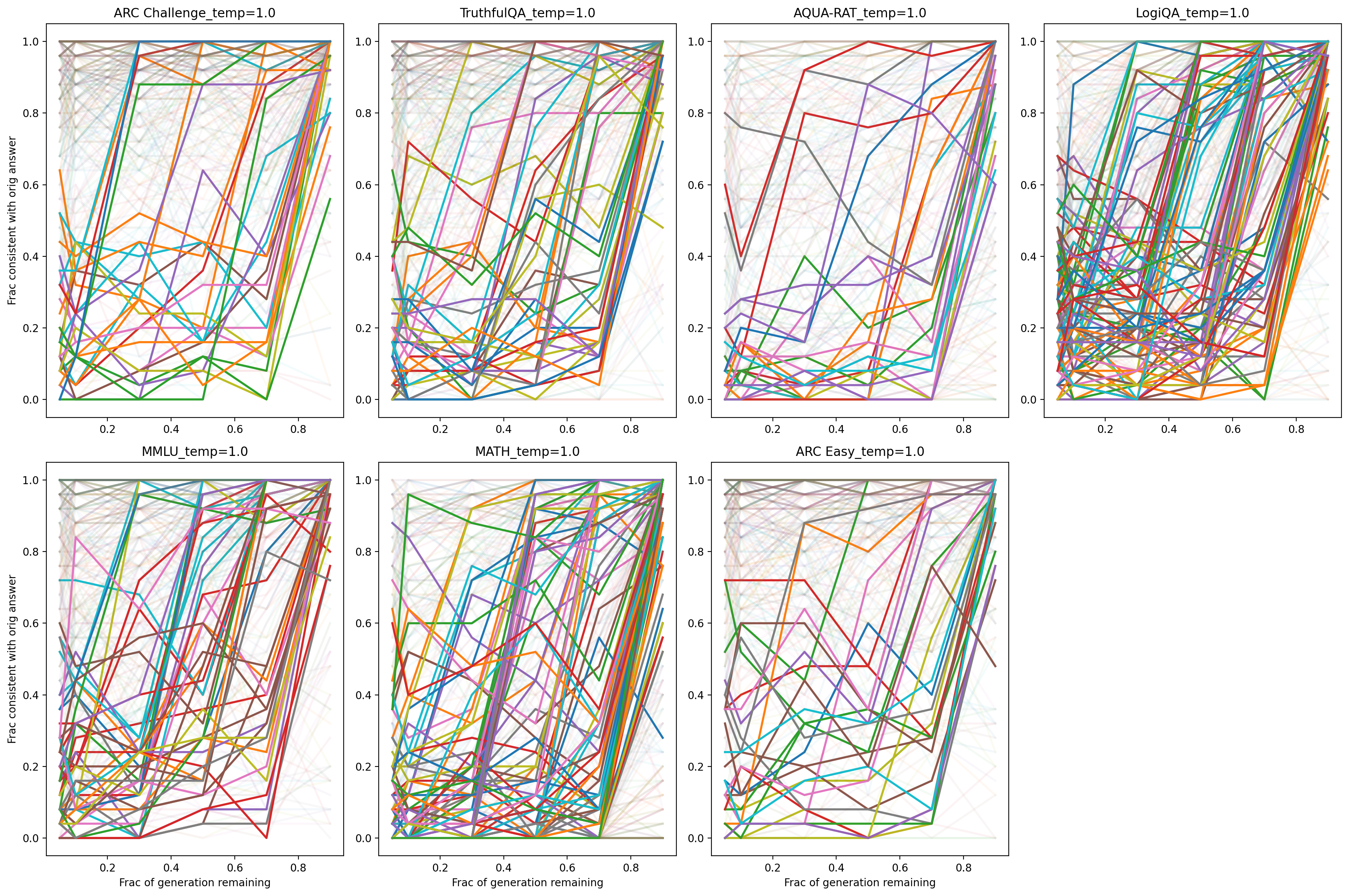
Figure 8: Probability that the answer is the same as a function of the percentage of the generation remaining for different math and reasoning benchmarks for Phi-$3$-$7$B-Instruct. Highlighted are generations with a 50% increase and no 30% decrease in the probability over one step.

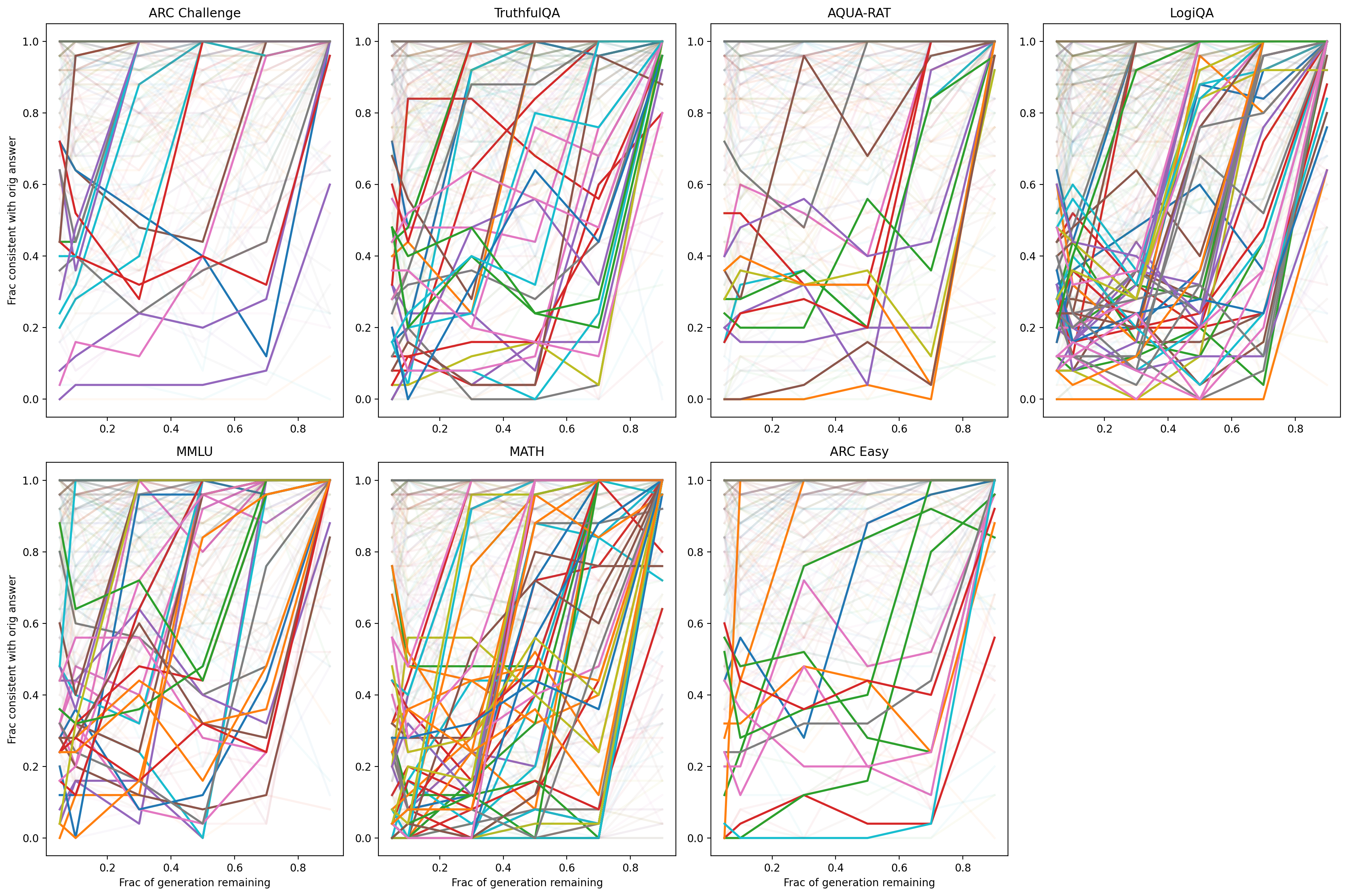
Figure 9: Probability that the answer is the same as a function of the percentage of the generation remaining for different math and reasoning benchmarks for Qwen-$2.5$-$7$B-Instruct. Highlighted are generations with a 50% increase and no 30% decrease in the probability over one step.

D.2.2 Comparison with directly answering for LLAMA-$3.1$-$8$B-Instruct

It is interesting to compare our approach in Figure 7 with that from [38], in which the model is directly asked for the answer (Figure 10). We can see that directly answering has a lower consistency than resampling across different amounts of generation remaining. Interestingly, the discrepancy is much higher for the math-datasets (MATH, AQUA) compared to extremely small difference in consistency for the other reasoning datasets. This may be because it is difficult to extract the answer from the middle of a chain of thought for math datasets than for other datasets.

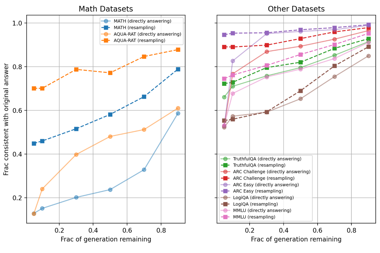
Figure 10: Difference between resampling to obtain the answer versus directly asking the model for the answer (as in [38]) for LLAMA-$3.1$-$8$B-Instruct.

D.2.3 Examples of critical windows

We provide a few more examples of critical windows (bolded).

D.2.4 Varied temperature sampling

In our above experiments with critical windows, we have been generating model responses at their default sampling temperatures: LLAMA-$3.1$-$8$B-Instruct: $0.6$, Phi-$3$-$7$B-Instruct: $1.0$, and Qwen-$2.5$-$7$B-Instruct: $0.7$. A natural question to ask is whether the sampling temperature affects the presence or strength of critical windows across these models. At one extreme, sampling at infinite temperature exhibits no critical windows since each token is generated uniformly at random. At the other extreme, zero temperature sampling is deterministic, so there is only one mode of behavior and critical windows again cannot exist. At intermediate temperatures, decreasing sampling temperature reduces token variance, so the sharpness of transition from general mixture to target submixture can be heightened. At the same time, reduced sampling variance also reduces the likelihood of transitioning between modes as well, leaving the overall effect on critical windows unclear.

First, we report the frequency of critical windows across the different temperatures for the MATH dataset: $0.1,0.4,0.7,$ and $1.0$. Then, we report the average size of a critical window on $400$ samples from MATH, running the forward-reverse experiment on each sample $25$ times and taking the max consecutive jump as the critical window size for that problem. From Figures 11 and 12, each model has its own relationship between temperature and critical window frequency and size, with no clear definite relationship across all models.

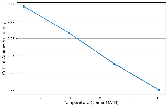
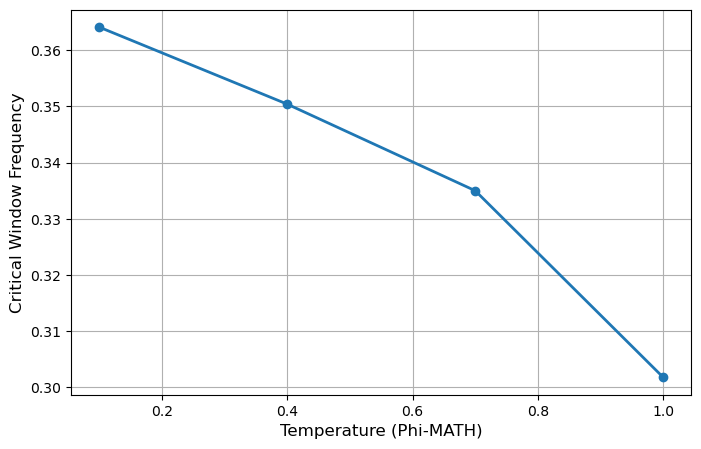
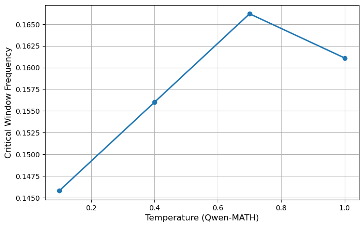
Figure 11: Temperature versus critical window frequency for  LLAMA-$3.1$-$8$B-Instruct, Phi-$3$-$7$B-Instruct, and Qwen-$2.5$-$7$B-Instruct.

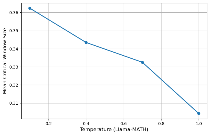
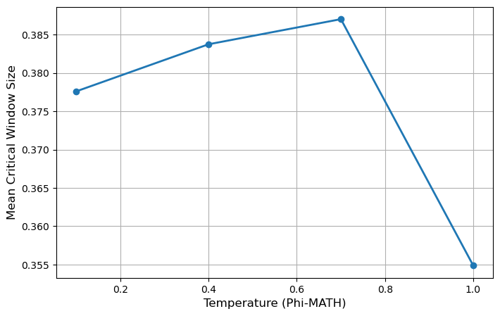
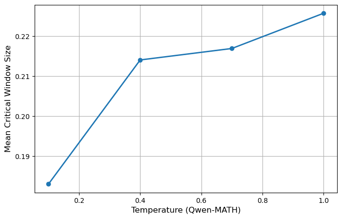
Figure 12: Temperature versus mean critical window size for  LLAMA-$3.1$-$8$B-Instruct, Phi-$3$-$7$B-Instruct, and Qwen-$2.5$-$7$B-Instruct.

References

- AAB+ [24] Marah Abdin, Jyoti Aneja, Harkirat Behl, Sébastien Bubeck, Ronen Eldan, Suriya Gunasekar, Michael Harrison, Russell J. Hewett, Mojan Javaheripi, Piero Kauffmann, James R. Lee, Yin Tat Lee, Yuanzhi Li, Weishung Liu, Caio C. T. Mendes, Anh Nguyen, Eric Price, Gustavo de Rosa, Olli Saarikivi, Adil Salim, Shital Shah, Xin Wang, Rachel Ward, Yue Wu, Dingli Yu, Cyril Zhang, and Yi Zhang. Phi-4 technical report, 2024.
- ADS+ [24] Cem Anil, Esin Durmus, Mrinank Sharma, Joe Benton, Sandipan Kundu, Joshua Batson, Nina Rimsky, Meg Tong, Jesse Mu, Daniel Ford, Francesco Mosconi, Rajashree Agrawal, Rylan Schaeffer, Naomi Bashkansky, Samuel Svenningsen, Mike Lambert, Ansh Radhakrishnan, Carson Denison, Evan J Hubinger, Yuntao Bai, Trenton Bricken, Timothy Maxwell, Nicholas Schiefer, Jamie Sully, Alex Tamkin, Tamera Lanham, Karina Nguyen, Tomasz Korbak, Jared Kaplan, Deep Ganguli, Samuel R. Bowman, Ethan Perez, Roger Grosse, and David Duvenaud. Many-shot jailbreaking. In Advances in the Thirty-Eighth Annual Conference on Neural Information Processing Systems, 2024.
- AJPG [24] Aryaman Arora, Dan Jurafsky, Christopher Potts, and Noah D. Goodman. Bayesian scaling laws for in-context learning, 2024.
- AK [23] Gabriel Alon and Michael Kamfonas. Detecting language model attacks with perplexity, 2023.
- ALL+ [19] Sanjeev Arora, Yuanzhi Li, Yingyu Liang, Tengyu Ma, and Andrej Risteski. A latent variable model approach to pmi-based word embeddings, 2019.
- AMS [23] Ahmed El Alaoui, Andrea Montanari, and Mark Sellke. Sampling from mean-field gibbs measures via diffusion processes. arXiv preprint arXiv:2310.08912, 2023.
- Ant [24] Anthropic. Developing a computer use model. https://www.anthropic.com/news/developing-computer-use, 2024.
- ASA+ [23] Ekin Akyürek, Dale Schuurmans, Jacob Andreas, Tengyu Ma, and Denny Zhou. What learning algorithm is in-context learning? investigations with linear models, 2023.
- BBdBM [24] Giulio Biroli, Tony Bonnaire, Valentin de Bortoli, and Marc Mézard. Dynamical regimes of diffusion models, 2024.
- BMR [20] Jean Barbier, Nicolas Macris, and Cynthia Rush. All-or-nothing statistical and computational phase transitions in sparse spiked matrix estimation, 2020.
- BSS+ [24] Luke Bailey, Alex Serrano, Abhay Sheshadri, Mikhail Seleznyov, Jordan Taylor, Erik Jenner, Jacob Hilton, Stephen Casper, Carlos Guestrin, and Scott Emmons. Obfuscated activations bypass llm latent-space defenses, 2024.
- CCE+ [18] Peter Clark, Isaac Cowhey, Oren Etzioni, Tushar Khot, Ashish Sabharwal, Carissa Schoenick, and Oyvind Tafjord. Think you have solved question answering? try arc, the ai2 reasoning challenge. arXiv preprint 1803.05457, 2018.
- CCL+ [23] Sitan Chen, Sinho Chewi, Jerry Li, Yuanzhi Li, Adil Salim, and Anru Zhang. Sampling is as easy as learning the score: theory for diffusion models with minimal data assumptions. In The Eleventh International Conference on Learning Representations, ICLR 2023, Kigali, Rwanda, May 1-5, 2023. OpenReview.net, 2023.
- CE [22] Yuansi Chen and Ronen Eldan. Localization schemes: A framework for proving mixing bounds for markov chains. In 2022 IEEE 63rd Annual Symposium on Foundations of Computer Science (FOCS), pages 110–122. IEEE, 2022.
- CLS+ [22] Jooyoung Choi, Jungbeom Lee, Chaehun Shin, Sungwon Kim, Hyunwoo Kim, and Sungroh Yoon. Perception prioritized training of diffusion models. In 2022 IEEE/CVF Conference on Computer Vision and Pattern Recognition (CVPR), pages 11462–11471, 2022.
- COGHK+ [22] Amin Coja-Oghlan, Oliver Gebhard, Max Hahn-Klimroth, Alexander S Wein, and Ilias Zadik. Statistical and computational phase transitions in group testing. In Po-Ling Loh and Maxim Raginsky, editors, Proceedings of Thirty Fifth Conference on Learning Theory, volume 178 of Proceedings of Machine Learning Research, pages 4764–4781. PMLR, 02–05 Jul 2022.
- CRD+ [23] Patrick Chao, Alexander Robey, Edgar Dobriban, Hamed Hassani, George J. Pappas, and Eric Wong. Jailbreaking black box large language models in twenty queries, 2023.
- DCX+ [23] Ning Ding, Yulin Chen, Bokai Xu, Yujia Qin, Zhi Zheng, Shengding Hu, Zhiyuan Liu, Maosong Sun, and Bowen Zhou. Enhancing chat language models by scaling high-quality instructional conversations, 2023.
- DLD+ [24] Qingxiu Dong, Lei Li, Damai Dai, Ce Zheng, Jingyuan Ma, Rui Li, Heming Xia, Jingjing Xu, Zhiyong Wu, Tianyu Liu, Baobao Chang, Xu Sun, Lei Li, and Zhifang Sui. A survey on in-context learning, 2024.
- EAMS [22] Ahmed El Alaoui, Andrea Montanari, and Mark Sellke. Sampling from the sherrington-kirkpatrick gibbs measure via algorithmic stochastic localization. In 2022 IEEE 63rd Annual Symposium on Foundations of Computer Science (FOCS), pages 323–334. IEEE, 2022.
- Eld [13] Ronen Eldan. Thin shell implies spectral gap up to polylog via a stochastic localization scheme. Geometric and Functional Analysis, 23(2):532–569, 2013.
- Eld [20] Ronen Eldan. Taming correlations through entropy-efficient measure decompositions with applications to mean-field approximation. Probability Theory and Related Fields, 176(3-4):737–755, 2020.
- Gem [24] Gemini. Challenges and solutions for aging adults. https://gemini.google.com/share/6d141b742a13, 2024.
- GPAM+ [14] Ian J. Goodfellow, Jean Pouget-Abadie, Mehdi Mirza, Bing Xu, David Warde-Farley, Sherjil Ozair, Aaron Courville, and Yoshua Bengio. Generative adversarial networks, 2014.
- gri [24] grimjim. Jailbroken llama-3.1-8b-instruct via lora. https://huggingface.co/grimjim/Llama-3.1-8B-Instruct-abliterated_via_adapter, 2024.
- GTLV [23] Shivam Garg, Dimitris Tsipras, Percy Liang, and Gregory Valiant. What can transformers learn in-context? a case study of simple function classes, 2023.
- GVS+ [23] Kristian Georgiev, Joshua Vendrow, Hadi Salman, Sung Min Park, and Aleksander Madry. The journey, not the destination: How data guides diffusion models. arXiv preprint arXiv:2312.06205, 2023.
- GZ [19] David Gamarnik and Ilias Zadik. High-dimensional regression with binary coefficients. estimating squared error and a phase transition, 2019.
- [29] Haize Labs. Automated multi-turn red-teaming with cascade. https://blog.haizelabs.com/posts/cascade, 2024.
- [30] Haize Labs. A trivial jailbreak against llama 3. https://github.com/haizelabs/llama3-jailbreak, 2024.
- HBB+ [21] Dan Hendrycks, Collin Burns, Steven Basart, Andy Zou, Mantas Mazeika, Dawn Song, and Jacob Steinhardt. Measuring massive multitask language understanding. In International Conference on Learning Representations, 2021.
- HBK+ [21] Dan Hendrycks, Collin Burns, Saurav Kadavath, Akul Arora, Steven Basart, Eric Tang, Dawn Song, and Jacob Steinhardt. Measuring mathematical problem solving with the math dataset, 2021.
- HJA [20] Jonathan Ho, Ajay Jain, and Pieter Abbeel. Denoising diffusion probabilistic models. Advances in Neural Information Processing Systems, 33:6840–6851, 2020.
- HMP [24] Brice Huang, Andrea Montanari, and Huy Tuan Pham. Sampling from spherical spin glasses in total variation via algorithmic stochastic localization. arXiv preprint arXiv:2404.15651, 2024.
- HXH [24] Luxi He, Mengzhou Xia, and Peter Henderson. What is in your safe data? identifying benign data that breaks safety, 2024.
- LC [24] Marvin Li and Sitan Chen. Critical windows: non-asymptotic theory for feature emergence in diffusion models, 2024.
- LCL+ [20] Jian Liu, Leyang Cui, Hanmeng Liu, Dandan Huang, Yile Wang, and Yue Zhang. Logiqa: A challenge dataset for machine reading comprehension with logical reasoning. In Christian Bessiere, editor, Proceedings of the Twenty-Ninth International Joint Conference on Artificial Intelligence, IJCAI-20, pages 3622–3628. International Joint Conferences on Artificial Intelligence Organization, 7 2020. Main track.
- LCR+ [23] Tamera Lanham, Anna Chen, Ansh Radhakrishnan, Benoit Steiner, Carson Denison, Danny Hernandez, Dustin Li, Esin Durmus, Evan Hubinger, Jackson Kernion, Kamilė Lukošiūtė, Karina Nguyen, Newton Cheng, Nicholas Joseph, Nicholas Schiefer, Oliver Rausch, Robin Larson, Sam McCandlish, Sandipan Kundu, Saurav Kadavath, Shannon Yang, Thomas Henighan, Timothy Maxwell, Timothy Telleen-Lawton, Tristan Hume, Zac Hatfield-Dodds, Jared Kaplan, Jan Brauner, Samuel R. Bowman, and Ethan Perez. Measuring faithfulness in chain-of-thought reasoning, 2023.
- LHE [22] Stephanie Lin, Jacob Hilton, and Owain Evans. TruthfulQA: Measuring how models mimic human falsehoods. In Proceedings of the 60th Annual Meeting of the Association for Computational Linguistics (Volume 1: Long Papers), pages 3214–3252, Dublin, Ireland, May 2022. Association for Computational Linguistics.
- LHS+ [24] Nathaniel Li, Ziwen Han, Ian Steneker, Willow Primack, Riley Goodside, Hugh Zhang, Zifan Wang, Cristina Menghini, and Summer Yue. Llm defenses are not robust to multi-turn human jailbreaks yet, 2024.
- LKB+ [23] Hunter Lightman, Vineet Kosaraju, Yura Burda, Harri Edwards, Bowen Baker, Teddy Lee, Jan Leike, John Schulman, Ilya Sutskever, and Karl Cobbe. Let’s verify step by step. arXiv preprint arXiv:2305.20050, 2023.
- LLX+ [24] Zicheng Lin, Tian Liang, Jiahao Xu, Xing Wang, Ruilin Luo, Chufan Shi, Siheng Li, Yujiu Yang, and Zhaopeng Tu. Critical tokens matter: Token-level contrastive estimation enhances llm’s reasoning capability, 2024.
- LME [24] Aaron Lou, Chenlin Meng, and Stefano Ermon. Discrete diffusion modeling by estimating the ratios of the data distribution, 2024.
- LRL+ [23] Bill Yuchen Lin, Abhilasha Ravichander, Ximing Lu, Nouha Dziri, Melanie Sclar, Khyathi Chandu, Chandra Bhagavatula, and Yejin Choi. The unlocking spell on base llms: Rethinking alignment via in-context learning, 2023.
- LXCX [24] Xiaogeng Liu, Nan Xu, Muhao Chen, and Chaowei Xiao. Autodan: Generating stealthy jailbreak prompts on aligned large language models. In The Twelfth International Conference on Learning Representations, 2024.
- LYDB [17] Wang Ling, Dani Yogatama, Chris Dyer, and Phil Blunsom. Program induction by rationale generation: Learning to solve and explain algebraic word problems. In Proceedings of the 55th Annual Meeting of the Association for Computational Linguistics (Volume 1: Long Papers), pages 158–167, Vancouver, Canada, July 2017. Association for Computational Linguistics.
- MHS+ [22] Chenlin Meng, Yutong He, Yang Song, Jiaming Song, Jiajun Wu, Jun-Yan Zhu, and Stefano Ermon. SDEdit: Guided image synthesis and editing with stochastic differential equations. In International Conference on Learning Representations, 2022.
- MNWS+ [23] Elchanan Mossel, Jonathan Niles-Weed, Youngtak Sohn, Nike Sun, and Ilias Zadik. Sharp thresholds in inference of planted subgraphs. In Gergely Neu and Lorenzo Rosasco, editors, Proceedings of Thirty Sixth Conference on Learning Theory, volume 195 of Proceedings of Machine Learning Research, pages 5573–5577. PMLR, 12–15 Jul 2023.
- [49] Andrea Montanari. Sampling, diffusions, and stochastic localization, 2023.
- [50] Andrea Montanari. Sampling, diffusions, and stochastic localization. arXiv preprint arXiv:2305.10690, 2023.
- MW [23] Andrea Montanari and Yuchen Wu. Posterior sampling from the spiked models via diffusion processes. arXiv preprint arXiv:2304.11449, 2023.
- NCH+ [23] Milad Nasr, Nicholas Carlini, Jonathan Hayase, Matthew Jagielski, A. Feder Cooper, Daphne Ippolito, Christopher A. Choquette-Choo, Eric Wallace, Florian Tramèr, and Katherine Lee. Scalable extraction of training data from (production) language models, 2023.
- NWZ [20] Jonathan Niles-Weed and Ilias Zadik. The all-or-nothing phenomenon in sparse tensor pca. In H. Larochelle, M. Ranzato, R. Hadsell, M.F. Balcan, and H. Lin, editors, Advances in Neural Information Processing Systems, volume 33, pages 17674–17684. Curran Associates, Inc., 2020.
- NWZ [23] Jonathan Niles-Weed and Ilias Zadik. It was "all" for "nothing": sharp phase transitions for noiseless discrete channels, 2023.
- PCT+ [23] Leonardo Petrini, Francesco Cagnetta, Umberto M Tomasini, Alessandro Favero, and Matthieu Wyart. How deep neural networks learn compositional data: The random hierarchy model. arXiv preprint arXiv:2307.02129, 2023.
- QPL+ [24] Xiangyu Qi, Ashwinee Panda, Kaifeng Lyu, Xiao Ma, Subhrajit Roy, Ahmad Beirami, Prateek Mittal, and Peter Henderson. Safety alignment should be made more than just a few tokens deep, 2024.
- RA [23] Gabriel Raya and Luca Ambrogioni. Spontaneous symmetry breaking in generative diffusion models. In Thirty-seventh Conference on Neural Information Processing Systems, 2023.
- RKV+ [24] Paul Röttger, Hannah Rose Kirk, Bertie Vidgen, Giuseppe Attanasio, Federico Bianchi, and Dirk Hovy. Xstest: A test suite for identifying exaggerated safety behaviours in large language models, 2024.
- Roo [01] B. Roos. Binomial approximation to the poisson binomial distribution: The krawtchouk expansion. Theory of Probability & Its Applications, 45(2):258–272, 2001.
- RXZ [19] Galen Reeves, Jiaming Xu, and Ilias Zadik. The all-or-nothing phenomenon in sparse linear regression, 2019.
- SC [16] Jonathan Scarlett and Volkan Cevher. Limits on support recovery with probabilistic models: An information-theoretic framework, 2016.
- SDCS [23] Yang Song, Prafulla Dhariwal, Mark Chen, and Ilya Sutskever. Consistency models, 2023.
- SFLW [24] Antonio Sclocchi, Alessandro Favero, Noam Itzhak Levi, and Matthieu Wyart. Probing the latent hierarchical structure of data via diffusion models, 2024.
- SFW [25] Antonio Sclocchi, Alessandro Favero, and Matthieu Wyart. A phase transition in diffusion models reveals the hierarchical nature of data. Proceedings of the National Academy of Sciences, 122(1):e2408799121, 2025.
- SLB+ [24] Alexandra Souly, Qingyuan Lu, Dillon Bowen, Tu Trinh, Elvis Hsieh, Sana Pandey, Pieter Abbeel, Justin Svegliato, Scott Emmons, Olivia Watkins, and Sam Toyer. A strongreject for empty jailbreaks, 2024.
- TAS [21] Lan V. Truong, Matthew Aldridge, and Jonathan Scarlett. On the all-or-nothing behavior of bernoulli group testing, 2021.
- TS [20] Lan V. Truong and Jonathan Scarlett. Support recovery in the phase retrieval model: Information-theoretic fundamental limits, 2020.
- [68] Roman Vershynin. High-Dimensional Probability: An Introduction with Applications in Data Science. Cambridge Series in Statistical and Probabilistic Mathematics. Cambridge University Press.
- vH [16] Ramon van Handel. Probability in high dimension. 2016.
- WHS [23] Alexander Wei, Nika Haghtalab, and Jacob Steinhardt. Jailbroken: How does llm safety training fail?, 2023.
- XRLM [22] Sang Michael Xie, Aditi Raghunathan, Percy Liang, and Tengyu Ma. An explanation of in-context learning as implicit bayesian inference, 2022.
- ZPW+ [24] Andy Zou, Long Phan, Justin Wang, Derek Duenas, Maxwell Lin, Maksym Andriushchenko, Rowan Wang, Zico Kolter, Matt Fredrikson, and Dan Hendrycks. Improving alignment and robustness with circuit breakers, 2024.
- ZW [24] Xiao Zhang and Ji Wu. Dissecting learning and forgetting in language model finetuning. In The Twelfth International Conference on Learning Representations, 2024.
- ZWC+ [23] Andy Zou, Zifan Wang, Nicholas Carlini, Milad Nasr, J. Zico Kolter, and Matt Fredrikson. Universal and transferable adversarial attacks on aligned language models, 2023.
- ZZX+ [24] Zhengyue Zhao, Xiaoyun Zhang, Kaidi Xu, Xing Hu, Rui Zhang, Zidong Du, Qi Guo, and Yunji Chen. Adversarial contrastive decoding: Boosting safety alignment of large language models via opposite prompt optimization, 2024.
- ZZYW [23] Yufeng Zhang, Fengzhuo Zhang, Zhuoran Yang, and Zhaoran Wang. What and how does in-context learning learn? bayesian model averaging, parameterization, and generalization, 2023.