Attention Sinks and Outlier Features:
A ‘Catch, Tag, and Release’ Mechanism for Embeddings

Abstract

Two prominent features of large language models (LLMs) is the presence of large-norm (outlier) features and the tendency for tokens to attend very strongly to a select few tokens. Despite often having no semantic relevance, these select tokens, called attention sinks, along with the large outlier features, have proven important for model performance, compression, and streaming. Consequently, investigating the roles of these phenomena within models and exploring how they might manifest in the model parameters has become an area of active interest. Through an empirical investigation, we demonstrate that attention sinks utilize outlier features to: catch a sequence of tokens, tag the captured tokens by applying a common perturbation, and then release the tokens back into the residual stream, where the tagged tokens are eventually retrieved. We prove that simple tasks, like averaging, necessitate the ‘catch, tag, release’ mechanism hence explaining why it would arise organically in modern LLMs. Our experiments also show that the creation of attention sinks can be completely captured in the model parameters using low-rank matrices, which has important implications for model compression and substantiates the success of recent approaches that incorporate a low-rank term to offset performance degradation. Link to project page.

1 Introduction

1.1 ‘Catch, Tag, and Release’ in Aquatic Conservation

In marine biology, the ‘catch, tag, and release’ mechanism is a vital tool for tracking fish populations. A fish is caught, fitted with a tracking tag encoding critical information, and then released back into a water stream, where it is monitored over time. This enables researchers to understand migration patterns, survival rates, and ecosystem interactions.

1.2 Pervasive Phenomena in LLMs

Remarkably, modern large language models (LLMs) exhibit a strikingly similar mechanism when processing tokens. To understand why, we first examine two recent discoveries in LLM research: Attention Sinks: Coined by Xiao et al. (2024), the authors found that all tokens attend strongly to the first token. Follow-up works demonstrated that sinks may also appear in later tokens (Yu et al., 2024; Sun et al., 2024a; Cancedda, 2024).

Outlier Features: Feature dimensions in the activations that are significantly larger in magnitude (Kovaleva et al., 2021; Dettmers et al., 2022). Unlike attention sinks, outlier feature dimensions are consistent across tokens.

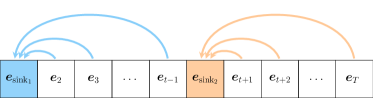
(a) Catch: Attention sinks catch the attention of a subset of tokens, through outlier features, as shown in Figures 2(a) and 2(b).

(b) Tag: The attention layer then tags the captured tokens by introducing an outlier feature dimension across all tokens. This shared tag causes tokens to cluster based on the attended sink, e.g. in PCA plots, as shown in Figure 2(c).

(c) Release: The tagged tokens are then released into the residual stream, where deeper layers can exploit the tag for further processing. This common tag induces token clustering even in deeper layers, e.g. in PCA plots, as shown in Figure 2(d).

Figure 1: An illustration of the ‘catch, tag, release’ mechanism.

Both phenomena have been linked to model performance, particularly in streaming (Xiao et al., 2024; Guo et al., 2024c), quantization techniques (Dettmers et al., 2022; Son et al., 2024; Ashkboos et al., 2024), and pruning techniques (Sun et al., 2024b; Zhang and Papyan, 2024), as behaviors that need to be preserved in the model’s attention weights and features. This, in turn, has driven prior research to investigate the following question.

1.3 Why Do Sinks and Outliers Emerge?

Existing answers generally fall into two main categories:

To Create Implicit Attention Biases

Models lack explicit bias parameters in the attention layers, leading attention sinks and large outliers to emerge as compensatory mechanisms that artificially introduce such biases. As a result, these effects can be mitigated by incorporating explicit key or value bias parameters (Sun et al., 2024a; Gu et al., 2024).

To Turn Off Attention Heads

Attention sinks emerge as a learned, data-dependent mechanism that disables an attention head when it is not needed for the current sequence (Bondarenko et al., 2023; Guo et al., 2024b).

1.4 Open Questions

Both perspectives still leave the following unanswered questions:

• How do attention sinks and outlier features manifest in model parameters?

While sinks and outlier features play a crucial role in model compression, prior research has primarily focused on their presence in model embeddings. Their manifestation within model parameters remains largely unexplored, raising questions about the best strategies for preserving these critical properties during compression.

• Why do attention sinks emerge in later tokens?

Neither perspective fully explains why attention sinks appear in later tokens alongside the first token sink (Yu et al., 2024; Cancedda, 2024). These sinks are sequence-dependent, contradicting the bias perspective, and the presence of multiple sinks seems unnecessary from the active-dormant perspective.

• Are attention sinks beneficial or better dispersed?

It remains unclear whether attention sinks are critical for model performance and need to be preserved (Xiao et al., 2024; Son et al., 2024), or if they should be dispersed or removed altogether (Sun et al., 2024a; Yu et al., 2024).

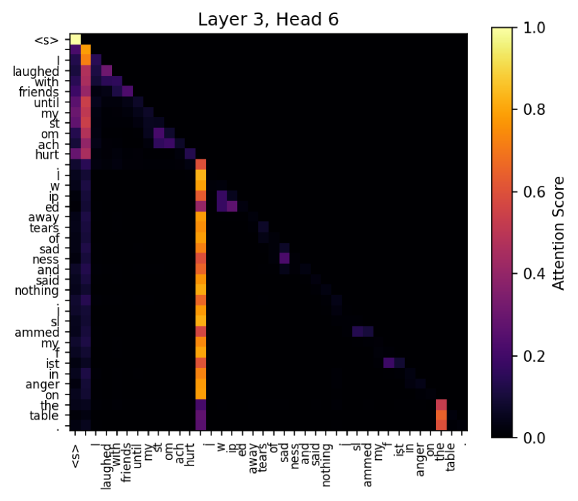
(a) Attention Weights. Two distinct attention sinks catch the attention of tokens appearing later in the sequence.

(b) Output of Attention Layer. The sink token exhibits an outlier feature that is then copied by the attention weights to the caught tokens, creating an outlier feature dimension.

(c) PCA on the output of the attention layer. Tokens cluster according to their attended sink: those attending to the first sink are shaded red, while those attending to the second sink are shaded green.

(d) PCA on the residual stream in a deep layer. Tagged tokens propagate through the residual stream, clustering based on their previously attended sink. Tokens that attended to the first sink are green, while those attending to the second sink are brown and yellow.

Figure 2: Visualization of the ‘catch, tag, and release’ mechanism. The second and third subplots use PCA-based coloring of embeddings.

1.5 Contributions

Our first contribution is a theoretical study of a two-layer attention model trained to average a sequence of numbers. This analysis answers the questions posed and establishes the following claims, summarized in the schematic below:

• A low-rank structure in the attention weight matrices, ${\bm{W}}_{Q},{\bm{W}}_{K},{\bm{W}}_{V}$, is responsible for attention sinks and outlier features.

• Attention sinks and outlier features are leveraged by the model to simulate a ‘catch, tag, and release’ mechanism, depicted and explained in Figure 1.

• The mechanism is useful for averaging a sequence, few-shot learning, and many other tasks.

Our second contribution involves showing that pruning algorithms that do not preserve low-rank structure in weight matrices, destroy attention sinks and feature outliers, harm the ‘catch, tag, release’ mechanism, and perform worse on few-shot learning.

1.6 Relationship with Prior Perspectives

The ‘catch, tag, and release’ mechanism does not contradict the perspectives on attention sinks presented in prior works by Sun et al. (2024a); Gu et al. (2024); Guo et al. (2024b). We hypothesize that the prior perspectives are accurately describing the behavior of the attention sink associated specifically with the first token in the sequence. The ‘catch, tag, and release’ mechanism expands on this by describing the behavior associated with the data-dependent sinks that emerge in later tokens (Yu et al., 2024).

2 Evidence for ‘Catch, Tag, Release’

This subsection provides empirical evidence for the existence of the ‘catch, tag, release’ mechanism. To this end, we input a prompt into the Phi-3 Medium model (Abdin et al., 2024), and compute various statistics, each offering evidence for the existence of a specific component of the mechanism.

Evidence for Catch

As described in Figure 1(a), the evidence of the catch mechanism amounts to showing the existence of an attention sink. We therefore save the attention weights of layer $3$, head $6$ and plot them in Figure 2(a). The visualization shows that there are indeed two sinks that are catching the attention of subsequent tokens.

Evidence for Tag

As described in Figure 1(b), demonstrating the tagging mechanism requires verifying token clustering based on the attended sink. Following Oquab et al. (2024), we compute the top two or three principal components of the $d\times d$ covariance matrix of the attention head outputs, where $d$ is the embedding dimension, and project the embeddings onto this basis. The projected values are then normalized to $[0,255]$ and mapped to RGB channels. Figure 2(c) illustrates the results, showing a clear grouping of tokens by their attention sinks.

Evidence for Release

As described in Figure 1(c), evidence for release amounts to showing that tokens in the residual stream in deeper layers have the same clustering behavior as exhibited in the attention head output. We therefore hook the inputs into the feedforward network in layer $17$, and apply the same PCA projection and normalization step as described earlier. The results, presented in Figure 2(d), reveal a similar grouping, providing evidence that the model has utilized the tags generated in the earlier layer.

Appendix B presents additional measurements using various prompts including chain-of-thought (Wei et al., 2022), zero-shot chain-of-thought (Brown et al., 2020), among others.

3 Intervention Through Model Pruning

This subsection aims to intervene at the root of the logical sequence, displayed in Section 1.5, namely the low-rank structure of the attention weight matrices and to test its effect on the attention sinks and outlier features, the ‘catch, tag, release’ mechanism, and ultimately performance on a down-stream task which relies on it: few-shot learning. The intervention is done through the use of pruning algorithms.

3.1 How is Pruning Related?

Pruning algorithms compress models by retaining the fewest possible nonzero parameters while preserving performance (Mozer and Smolensky, 1988; LeCun et al., 1989; Hassibi and Stork, 1992). However, they typically do not prioritize accurately capturing low-rank structures in the weights.

An exception to this is a recently proposed compression algorithm for LLMs, called OATS (Zhang and Papyan, 2024), which approximates the model’s weight matrices through a sparse-plus-low-rank decomposition:

$${\bm{W}}\approx\underbrace{{\bm{S}}}_{\text{Sparse}}+\underbrace{{\bm{U}}{\bm{V}}}_{\text{Low-Rank}}\!\!\!\!\mathrlap{{}^{\top}}\ \ .$$

This method, by design, explicitly preserves low-rank structures through the low-rank term, a key feature absent from traditional pruning algorithms.

Comparing pruning algorithms with OATS is therefore a natural intervention since it directly controls for the low-rank structure. Having established the intervention, we now test its effect on the attention sinks and outlier features.

3.2 Low-Rank Terms $\implies$ Sinks and Outliers

Figure 4 presents the attention weights for layer $2$, attention head $6$, of a Phi-3 Medium model in three configurations: a dense model, a model compressed by $50$% using OATS, and a model compressed by $50$% using OATS where the low-rank matrices for ${\bm{W}}_{Q},{\bm{W}}_{K},{\bm{W}}_{V}$ for that layer are set to $\bm{0}$. The plots reveal clear sinks and outliers, except in the model lacking low-rank terms, suggesting that the low-rank term in OATS is indeed responsible for both phenomena.

3.3 No Low-Rank Terms $\implies$ No Sinks and Outliers

Figure 5 compares the attention weights in layer $36$, head $16$, of a dense Phi-3 Medium model with models that are pruned by $50$% using OATS, and pruned by $50$% using Wanda (Sun et al., 2024b), and SparseGPT (Frantar and Alistarh, 2023) – two methods that do not prioritize a low-rank structure in their formulation. The visualizations reveal that pruning methods like Wanda and SparseGPT lack certain attention sinks found in both the dense and OATS models.

3.4 Sinks and Outliers $\implies$ ‘Catch, Tag, and Release’

The previous two subsections show that classical pruning algorithms fail to retain the low-rank components of attention weights, which results in the loss of attention sinks and outlier features. In contrast, OATS preserves them. Building on Section 2, which establishes the necessity of sinks and outliers for the ‘catch, tag, release’ mechanism, we conclude that pruning algorithms like Wanda and SparseGPT break the ‘catch, tag, release’ mechanism, whereas OATS maintains it.

3.5 ‘Catch, Tag, and Release’ $\implies$ Few-Shot Learning

Since the ‘catch, tag, release’ mechanism segments sequences, it is likely crucial for distinguishing between examples in few-shot learning. To test this, we measure the gap in $k$-shot performance on the MMLU dataset (Hendrycks et al., 2021) using LM Harness (Gao et al., 2024), where $k$ ranges from $0$ to $5$. We compare the performance of OATS with Wanda and SparseGPT in Figure 3.

Figure 3: Impact of increasing the number of examples on model performance. Accuracy is measured on the MMLU dataset using 50% pruned variants of the Phi-3 Medium model.

While all methods perform similarly at $0$-shot, where segmentation is less critical, the gap widens with $k$, highlighting the importance of OATS’ ability to retain the ‘catch, tag, release’ mechanism. In contrast, the model pruned by SparseGPT shows no improvement with more examples, indicating severely compromised few-shot capabilities.

(a) Dense

(b) Sparse $+$ Low-Rank

(c) Sparse $+\;\bm{0}$

Figure 4: Comparison of attention weights and attention output for layer $2$, head $6$, across the dense Phi-3 Medium, Phi-3 Medium compressed by the OATS algorithm, and Phi-3 Medium compressed by the OATS algorithm with only the sparse terms present in the current layer. The removal of the low-rank term from the ${\bm{W}}_{Q},{\bm{W}}_{K}$ fully removes the attention sinks that were present in both the dense model and the model compressed by OATS.

(a) Dense Model

(b) OATS

(c) Wanda

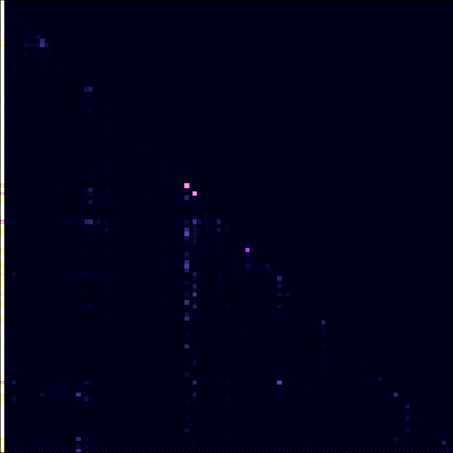
(d) SparseGPT

Figure 5: Visualizations of the attention weights of layer 36 head 16 of a Phi-3 Medium that has been compressed by $50$%. Pruning algorithms that do not prioritize a low-rank structure end up losing an attention sink that is present in both the dense model and OATS.

4 Theoretical Foundation

4.1 Setup and Main Result

Task

Given a sequence of $T$ tokens, consisting of numbers, $x_{i}\in\mathbb{R}$, separated by a special [SEP]token:

$${\bm{x}}=(x_{1},...,x_{t-1},\textnormal{{[SEP]}},x_{t+1},...,x_{T}),$$

the objective is to compute the average of the numbers appearing after the [SEP]token. To increase the complexity of the task, the position of the [SEP]token, denoted as $t$, varies across different sequences.

Embeddings

The number tokens are embedded into:

$${\bm{e}}_{i}=\texttt{Embed}(x_{i})=\begin{bmatrix}x_{i}\\ -1\end{bmatrix}\in\mathbb{R}^{2},\quad i\neq t,$$

while the [SEP] is embedded into:

$${\bm{e}}_{t}=\texttt{Embed}(\textnormal{{[SEP]}})=\begin{bmatrix}s_{\texttt{num}}\\ -s_{\texttt{tag}}\end{bmatrix}\in\mathbb{R}^{2},$$

where $s_{\texttt{num}},s_{\texttt{tag}}\in\mathbb{R}$ are learnable parameters. The first coordinate of the embeddings represents the numbers, while the second coordinate represents the tag.

The embeddings are concatenated into a matrix to form:

$${\bm{E}}=\begin{bmatrix}{\bm{e}}_{1}&{\bm{e}}_{2}&\cdots&{\bm{e}}_{T}\end{bmatrix}^{\top}\in\mathbb{R}^{T\times 2}.$$

Model

The embeddings are passed as input to a two-layer causal transformer:

$${\bm{H}} =\operatorname{Attention}({\bm{E}},{\bm{E}},{\bm{E}}{\bm{W}}^{1}_{V})+{\bm{E}}$$ (1)

$$f_{\theta}({\bm{x}}) =\operatorname{Attention}({\bm{h}}_{T}^{\top}{\bm{W}}^{2}_{Q},{\bm{H}}{\bm{W}}^{2}_{K},{\bm{H}}{\bm{W}}^{2}_{V}),$$ (2)

parameterized by:

$$\theta=({\bm{W}}^{1}_{V},{\bm{W}}^{2}_{Q},{\bm{W}}^{2}_{K},{\bm{W}}^{2}_{V},s_{\texttt{num}},s_{\texttt{tag}}).$$

We will use the auxiliary notation:

$${\bm{A}}^{1}=\operatorname{softmax}({\bm{E}}{\bm{E}}^{\top})$$

$${\bm{A}}^{2}=\operatorname{softmax}({\bm{H}}{\bm{W}}^{2}_{Q}{\bm{W}}^{2}_{K}{\bm{H}}^{\top}),$$

where the $\operatorname{softmax}(\cdot)$ is causal.

Theorem 4.1 (‘Catch, Tag, and Release’ Theory).

Assume the learnable parameters, $\theta$, satisfy: $\displaystyle s_{\texttt{num}}=0$ $\displaystyle{\bm{W}}^{1}_{V}=\begin{bmatrix}0&0\\ 0&-1\end{bmatrix}$ $\displaystyle{\bm{W}}^{2}_{Q}{\bm{W}}^{2}_{K}=\begin{bmatrix}0&b\\ 0&d\end{bmatrix},\ \ \text{where}\ \ d>0,b\in\mathbb{R}$ $\displaystyle{\bm{W}}^{2}_{V}=\begin{bmatrix}1\\ 0\end{bmatrix}$ (3) Then: $$f_{\theta}({\bm{x}})\stackrel{{\scriptstyle s_{\texttt{tag}}\to\infty}}{{\xrightarrow{\hskip 28.45274pt}}}\frac{1}{T-t}\sum_{i=t+1}^{T}x_{i}$$ for any $x_{1},...,x_{T}\in\mathbb{R}$. The model will have the following features for any sequence ${\bm{x}}$: • the ​​ [SEP] forms an attention sink, • the tokens after the ​​ [SEP] have activation outliers in their second coordinate, • the second coordinate is an outlier feature dimension, and • the attention matrices ${\bm{W}}^{1}_{V}$, ${\bm{W}}^{2}_{Q}$, ${\bm{W}}^{2}_{K}$, ${\bm{W}}^{2}_{V}$ are low rank, projecting either to the tag or number subspace

Remark 4.2.

The model utilizes a tagging mechanism based on the second coordinate of the token representations. A token is classified as:

  Untagged:

if its second coordinate is finite.

  Tagged:

if its second coordinate diverges.

Initially, all number tokens are assumed to be untagged, with their tag coordinate set to $-1$.

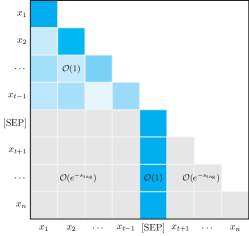
Figure 6: Attention probabilities in the first attention layer. The [SEP] token acts as an attention sink for tokens ${\bm{x}}_{i}$ with $i\geq t$. Consistent with Equation (4), the remaining probabilities in the same rows decay exponentially as $\mathcal{O}(e^{-s_{\texttt{tag}}})$. Notably, the attention sink does not influence the probabilities of tokens ${\bm{x}}_{i}$ for $i<t$, which remain $\mathcal{O}(1)$.

4.2 Proof of Theorem, Part 1: ‘Catch, Tag, Release’

The first part of the proof focuses on the first attention layer.

Catch Mechanism

The attention weight when token ${\bm{x}}_{i}$, for $i>t$ is attending to [SEP] is:

$${\bm{A}}^{1}_{i,t} =\frac{\exp({\bm{e}}_{i}^{\top}{\bm{e}}_{t})}{\sum_{k=1}^{T}\exp({\bm{e}}_{i}^{\top}{\bm{e}}_{k})}$$

$$=\frac{\exp({\bm{e}}_{i}^{\top}{\bm{e}}_{t})}{\exp({\bm{e}}_{i}^{\top}{\bm{e}}_{t})+\sum_{k=1,k\neq t}^{T}\exp({\bm{e}}_{i}^{\top}{\bm{e}}_{k})}$$

$$=\frac{\exp(x_{i}s_{\texttt{num}}+s_{\texttt{tag}})}{\exp(x_{i}s_{\texttt{num}}+s_{\texttt{tag}})+\sum_{k=1,k\neq t}^{i}\exp(x_{i}x_{k}+1)}$$

$$=\frac{\exp(s_{\texttt{tag}})}{\exp(s_{\texttt{tag}})+\sum_{k=1,k\neq t}^{i}\exp(x_{i}x_{k}+1)}\stackrel{{\scriptstyle s_{\texttt{tag}}\to\infty}}{{\xrightarrow{\hskip 28.45274pt}}}1.$$

Furthermore, for $i>t$ and $j\neq t$:

$${\bm{A}}^{1}_{i,j} =\frac{\exp(1+x_{i}x_{j})}{\exp(s_{\texttt{tag}})+\sum_{\begin{subarray}{c}k=1\\ k\neq j\end{subarray}}^{i}\exp(1+x_{i}x_{k})}\in\mathcal{O}(e^{-s_{\texttt{tag}}})$$ (4)

and therefore:

$${\bm{A}}^{1}_{i,j}\stackrel{{\scriptstyle s_{\texttt{tag}}\to\infty}}{{\xrightarrow{\hskip 28.45274pt}}}0\quad\text{for}\quad j\neq t.$$

Thus, [SEP]acts as an attention sink, where all tokens $x_{i}$ for $i>t$, as well as the [SEP] token itself, attend exclusively to the [SEP]token. As a result, the attention of all tokens $x_{i}$ for $i>t$ and the [SEP] token have been caught. These observations are depicted in Figure 6 above.

Tag Mechanism

The attention output of the $i$-th token for $i\geq t$ is:

$$\operatorname{Attention}({\bm{e}}_{i}^{\top},{\bm{E}},{\bm{E}}{\bm{W}}^{1}_{V})$$

$$= \sum_{j=1}^{i}{\bm{A}}^{1}_{i,j}{\bm{e}}_{j}^{\top}{\bm{W}}^{1}_{V}$$

$$= {\bm{A}}^{1}_{i,t}{\bm{e}}_{t}^{\top}{\bm{W}}^{1}_{V}+\sum_{j=1,j\neq t}^{i}{\bm{A}}^{1}_{i,j}{\bm{e}}_{j}^{\top}{\bm{W}}^{1}_{V}$$ (5)

$$= {\bm{A}}^{1}_{i,t}\begin{bmatrix}0&s_{\texttt{tag}}\end{bmatrix}+\sum_{j=1,j\neq t}^{i}{\bm{A}}^{1}_{i,j}{\bm{e}}_{j}^{\top}{\bm{W}}^{1}_{V}\stackrel{{\scriptstyle s_{\texttt{tag}}\to\infty}}{{\xrightarrow{\hskip 28.45274pt}}}\begin{bmatrix}0&\infty\end{bmatrix}.$$

Recall that the second coordinate of the embeddings represents the tag. The limit above implies that a tag has been created for all tokens $x_{i}$, for $i>t$.

After adding the tag to the residual stream, we obtain for $i>t$:

$${\bm{h}}_{i}={\bm{e}}_{i}+\operatorname{Attention}({\bm{e}}_{i}^{\top},{\bm{E}},{\bm{E}}{\bm{W}}^{1}_{V})^{\top}\stackrel{{\scriptstyle s_{\texttt{tag}}\to\infty}}{{\xrightarrow{\hskip 22.76228pt}}}\begin{bmatrix}x_{i}\\ \infty\end{bmatrix}$$ (6)

The above implies that all tokens, $x_{i}$, for $i>t$ have now been tagged.

Release Mechanism

The tagged tokens have now been released into the residual stream. As we will show in the next subsection, the tags will be leveraged by the second attention layer to generate the desired averaging mechanism.

4.3 Proof of Theorem, Part 2: Leveraging the Tags

The second part of the proof focuses on the second attention layer.

The attention weight when token $x_{T}$ is attending to token $x_{j}$ is given by:

$${\bm{A}}^{2}_{T,j} =\frac{\exp({\bm{h}}_{T}^{\top}{\bm{W}}^{2}_{Q}{\bm{W}}^{2}_{K}{\bm{h}}_{j})}{\sum_{k=1}^{T}\exp({\bm{h}}_{T}^{\top}{\bm{W}}^{2}_{Q}{\bm{W}}^{2}_{K}{\bm{h}}_{k})}.$$

Dividing the numerator and denominator by $\exp({\bm{h}}_{T}^{\top}{\bm{W}}^{2}_{Q}{\bm{W}}^{2}_{K}{\bm{h}}_{T})$, the expression becomes:

$${\bm{A}}^{2}_{T,j} =\frac{\exp({\bm{h}}_{T}^{\top}{\bm{W}}^{2}_{Q}{\bm{W}}^{2}_{K}{\bm{h}}_{j}-{\bm{h}}_{T}^{\top}{\bm{W}}^{2}_{Q}{\bm{W}}^{2}_{K}{\bm{h}}_{T})}{\sum_{k=1}^{T}\exp({\bm{h}}_{T}^{\top}{\bm{W}}^{2}_{Q}{\bm{W}}^{2}_{K}{\bm{h}}_{k}-{\bm{h}}_{T}^{\top}{\bm{W}}^{2}_{Q}{\bm{W}}^{2}_{K}{\bm{h}}_{T})}$$

$$=\frac{\exp({\bm{h}}_{T}^{\top}{\bm{W}}^{2}_{Q}{\bm{W}}^{2}_{K}({\bm{h}}_{j}-{\bm{h}}_{T}))}{\sum_{k=1}^{T}\exp({\bm{h}}_{T}^{\top}{\bm{W}}^{2}_{Q}{\bm{W}}^{2}_{K}({\bm{h}}_{k}-{\bm{h}}_{T}))}.$$ (7)

Consider the term inside the exponent:

$${\bm{h}}_{T}^{\top}{\bm{W}}^{2}_{Q}{\bm{W}}^{2}_{K}({\bm{h}}_{j}-{\bm{h}}_{T}).$$

There are three cases for $j$, depending on whether it is less than, equal to, or greater than $t$. In the next subsection, we prove that

Case 1:

For $j<t$ (non-tagged tokens),

$$\exp({\bm{h}}_{T}^{\top}{\bm{W}}^{2}_{Q}{\bm{W}}^{2}_{K}({\bm{h}}_{j}-{\bm{h}}_{T}))\stackrel{{\scriptstyle s_{\texttt{tag}}\to\infty}}{{\xrightarrow{\hskip 28.45274pt}}}0.$$

Case 2:

For $j=t$ (sink token),

$$\exp({\bm{h}}_{T}^{\top}{\bm{W}}^{2}_{Q}{\bm{W}}^{2}_{K}({\bm{h}}_{t}-{\bm{h}}_{T}))\stackrel{{\scriptstyle s_{\texttt{tag}}\to\infty}}{{\xrightarrow{\hskip 28.45274pt}}}0.$$

Case 3:

For $j>t$ (tagged tokens),

$$\exp({\bm{h}}_{T}^{\top}{\bm{W}}^{2}_{Q}{\bm{W}}^{2}_{K}({\bm{h}}_{j}-{\bm{h}}_{T}))\stackrel{{\scriptstyle s_{\texttt{tag}}\to\infty}}{{\xrightarrow{\hskip 28.45274pt}}}1.$$

Combining all three cases together with Equation (7) leads to:

$$\lim_{s_{\texttt{tag}}\to\infty}{\bm{A}}^{2}_{T,j}=\begin{cases}0,&j<t\\ 0,&j=t\\ \frac{1}{T-t},&j>t\\ \end{cases}$$

The above shows how the tags have been leveraged to arrive at a uniform distribution over the desired tokens. Then using this, Equation (6), and Equation (3), we can conclude that:

$$f_{\theta}({\bm{x}})\stackrel{{\scriptstyle s_{\texttt{tag}}\to\infty}}{{\xrightarrow{\hskip 28.45274pt}}}\frac{1}{T-t}\sum_{i=1}^{T}x_{i}.$$

4.4 Proof of Theorem, Part 3: Proving the Three Cases

Combining Equation (5) and Equation (6), we get for all $1\leq i\leq T$:

$${\bm{h}}_{i}^{\top} ={\bm{e}}_{i}^{\top}+{\bm{A}}^{1}_{i,t}{\bm{e}}_{t}^{\top}{\bm{W}}^{1}_{V}+\sum_{\begin{subarray}{c}k=1\\ k\neq t\end{subarray}}^{i}{\bm{A}}^{1}_{i,k}{\bm{e}}_{k}^{\top}{\bm{W}}^{1}_{V},$$

and specifically:

$${\bm{h}}_{T}^{\top}={\bm{e}}_{T}^{\top}+{\bm{A}}^{1}_{T,t}{\bm{e}}_{t}^{\top}{\bm{W}}^{1}_{V}+\underbrace{\sum_{\begin{subarray}{c}k=1\\ k\neq t\end{subarray}}^{T}{\bm{A}}^{1}_{T,k}{\bm{e}}_{k}^{\top}{\bm{W}}^{1}_{V}}_{\mathcal{O}(e^{-s_{\texttt{tag}}})}$$

$$\implies {\bm{h}}_{T}=\begin{bmatrix}x_{T}\\ -1\end{bmatrix}+{\bm{A}}^{1}_{T,t}\begin{bmatrix}0\\ s_{\texttt{tag}}\end{bmatrix}+\mathcal{O}(e^{-s_{\texttt{tag}}}).$$

Using the two equations above, we get for all $1\leq j\leq T$:

$${\bm{h}}_{j}^{\top}-{\bm{h}}_{T}^{\top} ={\bm{e}}_{j}^{\top}-{\bm{e}}_{T}^{\top}+({\bm{A}}^{1}_{j,t}-{\bm{A}}^{1}_{T,t}){\bm{e}}_{t}^{\top}{\bm{W}}^{1}_{V}$$

$$\quad+\underbrace{\sum_{\begin{subarray}{c}k=1\\ k\neq t\end{subarray}}^{j}{\bm{A}}^{1}_{j,k}{\bm{e}}_{k}^{\top}{\bm{W}}^{1}_{V}}_{\mathcal{O}(1)\text{ if }j<t,\text{ otherwise }\mathcal{O}(e^{-s_{\texttt{tag}}})}-\underbrace{\sum_{\begin{subarray}{c}k=1\\ k\neq t\end{subarray}}^{T}{\bm{A}}^{1}_{T,k}{\bm{e}}_{k}^{\top}{\bm{W}}^{1}_{V},}_{\mathcal{O}(e^{-s_{\texttt{tag}}})}$$

where the order of magnitude of the last two terms is given by Equation (4) and depicted in Figure 6.

Additionally, we will use the fact that for all $j\geq t$:

$$\lim_{s_{\texttt{tag}}\to\infty}d\cdot{\bm{A}}^{1}_{T,t}({\bm{A}}^{1}_{j,t}-{\bm{A}}^{1}_{T,t})s_{\texttt{tag}}^{2}=0,$$

which we show in Appendix A.

Case 1:

For $j<t$ (non-tagged tokens),

$${\bm{h}}_{T}^{\top}{\bm{W}}^{2}_{Q}{\bm{W}}^{2}_{K}({\bm{h}}_{j}-{\bm{h}}_{T})$$

$$={\bm{h}}_{T}^{\top}{\bm{W}}^{2}_{Q}{\bm{W}}^{2}_{K}\left(\begin{bmatrix}x_{j}-x_{T}\\ 0\end{bmatrix}-{\bm{A}}^{1}_{T,t}\begin{bmatrix}0\\ s_{\texttt{tag}}\end{bmatrix}+\mathcal{O}(1)\right)$$

$$={\bm{h}}_{T}^{\top}\left(-{\bm{A}}^{1}_{T,t}\begin{bmatrix}b\cdot s_{\texttt{tag}}\\ d\cdot s_{\texttt{tag}}\end{bmatrix}+\mathcal{O}(1)\right)$$

$$=\left(\begin{bmatrix}x_{T}\\ -1\end{bmatrix}+{\bm{A}}^{1}_{T,t}\begin{bmatrix}0\\ s_{\texttt{tag}}\end{bmatrix}+\mathcal{O}(e^{-s_{\texttt{tag}}})\right)^{\top}$$

$$\phantom{=}\quad\left(-{\bm{A}}^{1}_{T,t}\begin{bmatrix}b\cdot s_{\texttt{tag}}\\ d\cdot s_{\texttt{tag}}\end{bmatrix}+\mathcal{O}(1)\right)$$

$$=-({\bm{A}}^{1}_{T,t})^{2}\cdot d\cdot s_{\texttt{tag}}^{2}+\mathcal{O}(s_{\texttt{tag}})$$

$$\stackrel{{\scriptstyle s_{\texttt{tag}}\to\infty}}{{\xrightarrow{\hskip 28.45274pt}}}-\infty,\text{ since }d>0.$$

Case 2:

For $j=t$ (sink token),

$${\bm{h}}_{T}^{\top}{\bm{W}}^{2}_{Q}{\bm{W}}^{2}_{K}({\bm{h}}_{t}-{\bm{h}}_{T})$$

$$={\bm{h}}_{T}^{\top}{\bm{W}}^{2}_{Q}{\bm{W}}^{2}_{K}\bigg{(}\begin{bmatrix}0-x_{T}\\ -s_{\texttt{tag}}+1\end{bmatrix}$$

$$\qquad+({\bm{A}}^{1}_{t,t}-{\bm{A}}^{1}_{T,t})\begin{bmatrix}0\\ s_{\texttt{tag}}\end{bmatrix}\quad+\mathcal{O}(e^{-s_{\texttt{tag}}})\bigg{)}$$

$$={\bm{h}}_{T}^{\top}\bigg{(}\begin{bmatrix}b\cdot(1-s_{\texttt{tag}})\\ d\cdot(1-s_{\texttt{tag}})\end{bmatrix}$$

$$\qquad+({\bm{A}}^{1}_{t,t}-{\bm{A}}^{1}_{T,t})\begin{bmatrix}b\cdot s_{\texttt{tag}}\\ d\cdot s_{\texttt{tag}}\end{bmatrix}+\mathcal{O}(e^{-s_{\texttt{tag}}})\bigg{)}$$

$$=-{\bm{A}}^{1}_{T,t}\cdot d\cdot s_{\texttt{tag}}^{2}$$

$$\qquad+\underbrace{d\cdot{\bm{A}}^{1}_{T,t}({\bm{A}}^{1}_{t,t}-{\bm{A}}^{1}_{T,t})s_{\texttt{tag}}^{2}}_{\stackrel{{\scriptstyle s_{\texttt{tag}}\to\infty}}{{\xrightarrow{\hskip 28.45274pt}}}0}+\mathcal{O}(s_{\texttt{tag}})$$

$$\stackrel{{\scriptstyle s_{\texttt{tag}}\to\infty}}{{\xrightarrow{\hskip 28.45274pt}}}-\infty.$$

Case 3:

For $j>t$ (tagged tokens),

$${\bm{h}}_{T}^{\top}{\bm{W}}^{2}_{Q}{\bm{W}}^{2}_{K}({\bm{h}}_{j}-{\bm{h}}_{T})$$

$$={\bm{h}}_{T}^{\top}{\bm{W}}^{2}_{Q}{\bm{W}}^{2}_{K}\bigg{(}\begin{bmatrix}x_{j}-x_{T}\\ 0\end{bmatrix}+$$

$$\qquad+({\bm{A}}^{1}_{j,t}-{\bm{A}}^{1}_{T,t})\begin{bmatrix}0\\ s_{\texttt{tag}}\end{bmatrix}+\mathcal{O}(e^{-s_{\texttt{tag}}})\bigg{)}$$

$$={\bm{h}}_{T}^{\top}\left(({\bm{A}}^{1}_{j,t}-{\bm{A}}^{1}_{T,t})\begin{bmatrix}b\cdot s_{\texttt{tag}}\\ d\cdot s_{\texttt{tag}}\end{bmatrix}+\mathcal{O}(e^{-s_{\texttt{tag}}})\right)$$

$$=({\bm{A}}^{1}_{j,t}-{\bm{A}}^{1}_{T,t})(x_{T}\cdot b\cdot s_{\texttt{tag}}-d\cdot s_{\texttt{tag}})$$

$$\quad+d\cdot{\bm{A}}^{1}_{T,t}({\bm{A}}^{1}_{j,t}-{\bm{A}}^{1}_{T,t})s_{\texttt{tag}}^{2}$$

$$\quad+\mathcal{O}(s_{\texttt{tag}}e^{-s_{\texttt{tag}}})$$

$$\stackrel{{\scriptstyle s_{\texttt{tag}}\to\infty}}{{\xrightarrow{\hskip 28.45274pt}}}0,$$

where $\lim_{s_{\texttt{tag}}\to\infty}({\bm{A}}^{1}_{j,t}-{\bm{A}}^{1}_{T,T})s_{\texttt{tag}}=0$ is proved in Appendix A.

5 Related Work

Register Buffers in Transformers

Darcet et al. (2024) observed that vision transformers exhibit high-norm outlier tokens, similar to LLMs, and that registers (data-independent tokens) are needed to prevent them from arising. This aligns closely with the perspective proposed by Sun et al. (2024a); Gu et al. (2024) that the first token attention sink is serving as a bias term for the attention mechanism.

Adam Causes Sinks and Outliers

Another recent avenue of investigation is whether attention sinks and outlier feature dimensions are a by-product of the optimizer. Both Kaul et al. (2024) and Guo et al. (2024b), show that the Adam optimizer (Kingma and Ba, 2015) leads to attention sinks and outlier features. In the former, they propose OrthoAdam which applies a rotation to the gradients to prevent any specific outlier dimensions.

Rank Collapse

Recent studies have shown that stacking self-attention layers in transformers can lead to rank collapse, where token representations lose dimensionality due to inherent architectural properties (Noci et al., 2022; Geshkovski et al., 2024). This phenomenon may stem from the ‘catch, tag, release’ mechanism, in which attention concentrates around attention sinks, causing tokens to cluster around them and become confined to a low-rank subspace.

Low-Rank Terms for Model Compression

Beyond OATS, other works have also proposed leveraging low-rank terms to mitigate compression loss for deep networks (Yu et al., 2017; Mozaffari and Dehnavi, 2024; Li et al., 2025). Another line of research is to incorporate a low-rank adapter during compression that is fine-tuned to mitigate drops in performance (Li et al., 2023; Zhang et al., 2023; Guo et al., 2024a; Zhao et al., 2024; Mozaffari et al., 2025).

6 Conclusion

This paper establishes that low-rank structures in attention weight matrices cause attention sinks and outlier features, which, in turn, enable the ‘catch, tag, and release’ mechanism. This mechanism serves as a fundamental organizational principle in transformers, dynamically segmenting and tagging token sequences to facilitate tasks such as few-shot learning and chain-of-thought reasoning. Empirically, we demonstrate that pruning techniques that fail to preserve low-rank structures disrupt this mechanism, significantly impairing few-shot generalization. Through rigorous theoretical analysis, we prove that ‘catch, tag, and release’ is not incidental but necessary for performing fundamental tasks like averaging a sub-sequence of numbers. This provides a compelling explanation for why this phenomenon emerges organically in transformer architectures.

Appendix A Proof of Auxiliary Limits

We first show that:

$$\lim_{s_{\texttt{tag}}\to\infty}d\cdot{\bm{A}}^{1}_{T,t}({\bm{A}}^{1}_{t,t}-{\bm{A}}^{1}_{T,t})s_{\texttt{tag}}^{2}=0$$

By definition:

$${\bm{A}}^{1}_{T,t}=\frac{\exp(s_{\texttt{tag}})}{\exp(s_{\texttt{tag}})+\sum_{k=1,k\neq t}^{T}\exp(x_{T}x_{k}+1)}=\frac{1}{1+\sum_{k=1,k\neq t}^{T}\exp(x_{T}x_{k}+1-s_{\texttt{tag}})}$$

and that:

$${\bm{A}}^{1}_{t,t}=\frac{\exp(s_{\texttt{tag}}^{2})}{\exp(s_{\texttt{tag}}^{2})+(t-1)\exp(s_{\texttt{tag}})}=\frac{1}{1+(t-1)\exp(s_{\texttt{tag}}-s_{\texttt{tag}}^{2})}.$$

Thus,

$${\bm{A}}^{1}_{t,t}-{\bm{A}}^{1}_{T,t}=\frac{\sum_{k=1,k\neq t}^{T}\exp(x_{T}x_{k}+1-s_{\texttt{tag}})-(t-1)\exp(s_{\texttt{tag}}-s_{\texttt{tag}}^{2})}{\left(1+(t-1)\exp(s_{\texttt{tag}}-s_{\texttt{tag}}^{2})\right)\cdot\left(1+\sum_{k=1,k\neq t}^{T}\exp(x_{T}x_{k}+1-s_{\texttt{tag}})\right)}$$

Then:

$$\lim_{s_{\texttt{tag}}\to\infty}s_{\texttt{tag}}^{2}({\bm{A}}^{1}_{t,t}-{\bm{A}}^{1}_{T,t})=\lim_{s_{\texttt{tag}}\to\infty}\frac{\sum_{k=1,k\neq t}^{T}s_{\texttt{tag}}^{2}\exp(x_{T}x_{k}+1-s_{\texttt{tag}})-(t-1)s_{\texttt{tag}}^{2}\exp(s_{\texttt{tag}}-s_{\texttt{tag}}^{2})}{\left(1+(t-1)\exp(s_{\texttt{tag}}-s_{\texttt{tag}}^{2})\right)\cdot\left(1+\sum_{k=1,k\neq t}^{T}\exp(x_{T}x_{k}+1-s_{\texttt{tag}})\right)}=\frac{0}{1}=0$$

The rest follows from the fact that $\lim_{s_{\texttt{tag}}\to\infty}{\bm{A}}^{1}_{T,t}=1$ and applying basic limit laws.

We now show similarly that for $j>t$:

$$\lim_{s_{\texttt{tag}}\to\infty}({\bm{A}}^{1}_{j,t}-{\bm{A}}^{1}_{T,T})s_{\texttt{tag}}=0,\qquad\lim_{s_{\texttt{tag}}\to\infty}({\bm{A}}^{1}_{j,t}-{\bm{A}}^{1}_{T,T})s_{\texttt{tag}}^{2}=0$$

Observe that for $j>t$:

$${\bm{A}}^{1}_{j,t}=\frac{\exp(s_{\texttt{tag}})}{\exp(s_{\texttt{tag}})+\sum_{k=1,k\neq t}^{j}\exp(x_{j}x_{k}+1)}=\frac{1}{1+\sum_{k=1,k\neq t}^{j}\exp(x_{j}x_{k}+1-s_{\texttt{tag}})}$$

Then

$$\lim_{s_{\texttt{tag}}\to\infty}({\bm{A}}^{1}_{j,t}-{\bm{A}}^{1}_{T,T})s_{\texttt{tag}} =\frac{\sum_{k=1,k\neq t}^{T}s_{\texttt{tag}}\exp(x_{T}x_{k}+1-s_{\texttt{tag}})-\sum_{k=1,k\neq t}^{j}s_{\texttt{tag}}\exp(x_{j}x_{k}+1-s_{\texttt{tag}})}{\left(1+\sum_{k=1,k\neq t}^{j}\exp(x_{j}x_{k}+1-s_{\texttt{tag}})\right)\cdot\left(1+\sum_{k=1,k\neq t}^{T}\exp(x_{T}x_{k}+1-s_{\texttt{tag}})\right)}$$

$$=\frac{0}{1}=0$$

and similarly,

$$\lim_{s_{\texttt{tag}}\to\infty}({\bm{A}}^{1}_{j,t}-{\bm{A}}^{1}_{T,T})s_{\texttt{tag}}^{2} =\frac{\sum_{k=1,k\neq t}^{T}s_{\texttt{tag}}^{2}\exp(x_{T}x_{k}+1-s_{\texttt{tag}})-\sum_{k=1,k\neq t}^{j}s_{\texttt{tag}}^{2}\exp(x_{j}x_{k}+1-s_{\texttt{tag}})}{\left(1+\sum_{k=1,k\neq t}^{j}\exp(x_{j}x_{k}+1-s_{\texttt{tag}})\right)\cdot\left(1+\sum_{k=1,k\neq t}^{T}\exp(x_{T}x_{k}+1-s_{\texttt{tag}})\right)}$$

$$=\frac{0}{1}=0$$

Appendix B Further Experimental Results

(a) Input embedding visualization at layer 3. The visualization does not display any meaningful clustering prior to the tagging mechanism.

(b) Attention probabilities at layer 3, head 30.

(c) Activation outliers in attention output at layer 3, head 30.

(d) Value embedding at layer 3, head 30.

(e) PCA on residual stream at layer 18.

Figure 7: Visualization of the ‘catch, tag, release’ mechanism on a sample prompt.

(a) PCA on the input embeddings to attention layer 3.

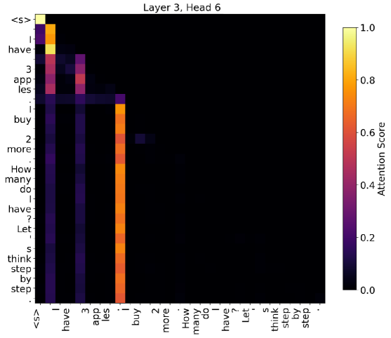
(b) Attention weights of layer 3, head 6.

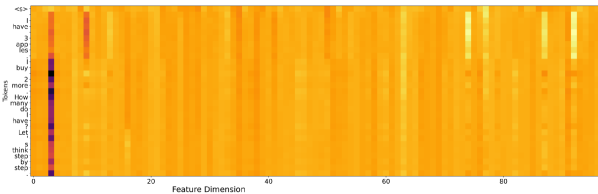
(c) Output of attention layer 3, head 6.

(d) PCA on the output of attention layer 3, head 6.

(e) PCA on the residual stream at layer 3 after the attention layer.

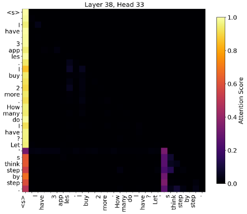
(f) Attention sink at layer 38, head 33,
highlighting “Let’s think step by step”.

(g) PCA on the residual stream at layer 38, preserving earlier tagging effects.

Figure 8: Visualization of the ‘catch, tag, release’ mechanism in Zero-Shot Chain of Thought (CoT) prompt. Later layers reveal an attention sink forming on “Let’s think step by step”, with the output embedding reflecting earlier tagged value embeddings.

(a) PCA on the input embeddings to attention layer 5.

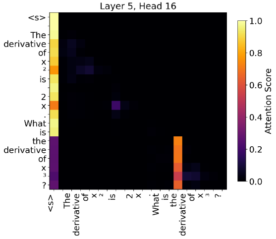
(b) Attention weights of layer 5, head 16.

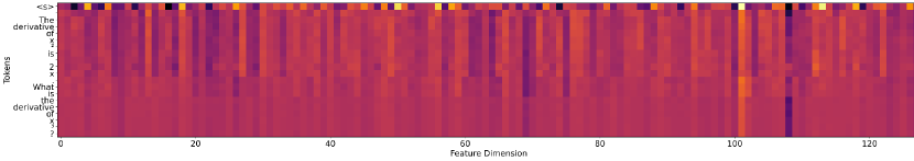
(c) Output of attention layer 5, head 16.

(d) PCA on the output of attention layer 5, head 16.

(e) PCA on the residual stream at layer 21.

Figure 9: Visualization of the ‘catch, tag, release’ mechanism on a Chain of Thought (CoT) prompt.

(a) PCA on the input embeddings to attention layer 5.

(b) Attention weights at layer 5, head 14.

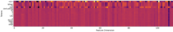
(c) Output of attention layer 5, head 14.

(d) PCA on the output of attention layer 5, head 14.

(e) PCA on the residual stream at layer 18.

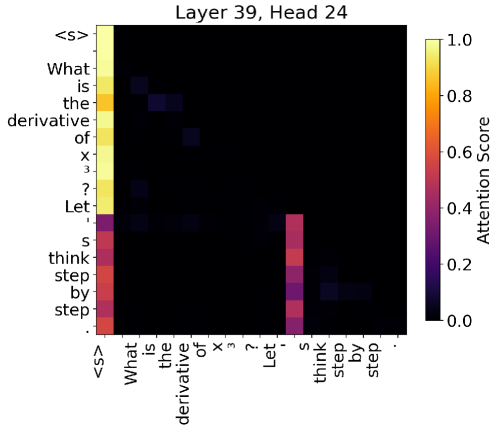
(f) Attention sink at layer 39, head 24,
highlighting “Let’s think step by step”.

(g) PCA on residual stream at layer 39, preserving earlier tagging effects.

Figure 10: Visualization of the ‘catch, tag, release’ mechanism on a Zero-Shot Chain of Thought (CoT) prompt. Later layers reveal an attention sink forming on ”Let’s think step by step”, with the output embedding retaining features from tagged value embeddings.

(a) PCA on the input embeddings to attention layer 3.

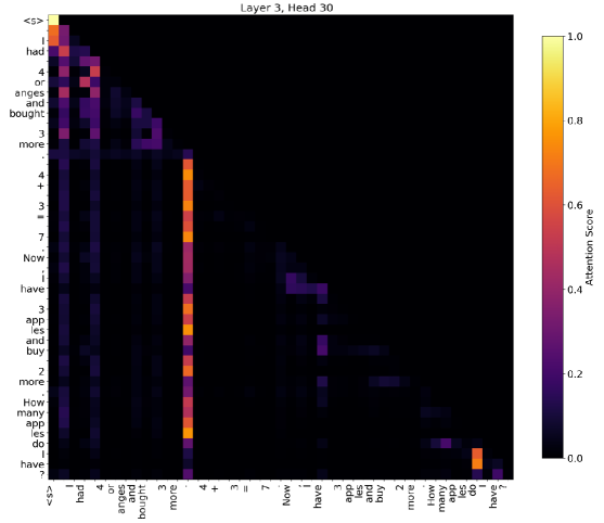
(b) Attention weights of layer 3, head 30.

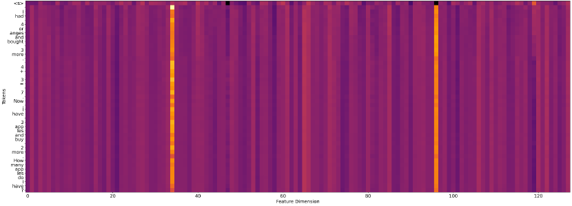
(c) Output of attention layer 3, head 30.

(d) PCA on the output of attention layer 3, head 30.

(e) PCA on the residual stream at layer 16.

Figure 11: Visualization of the ‘catch, tag, release’ mechanism on a Chain of Thought (CoT) prompt.

Appendix C Experiment Details

We use the HuggingFace Transformers library to load the models utilized in our experiments [Wolf et al., 2019].

C.1 Pruning Hyperparameters

For all pruning experiments, we prune uniformly across all linear layers in the model, excluding the embedding and head layers, remaining consistent with [Frantar and Alistarh, 2023, Sun et al., 2024b, Zhang and Papyan, 2024]. As calibration data, we use 128 sequences of length 2048 from the first shard of the C4 dataset [Raffel et al., 2019]. The algorithm-specific hyperparameters are:

• SparseGPT

  • Hessian Dampening: $0.1$

  • Block Size: $128$

• OATS

  • Iterations: $80$

  • Rank Ratio: $0.25$

The prompt used to generate Figure 5 is:

Read the following paragraph and determine if the hypothesis is true. \n \n Premise: A: Oh, oh yeah, and every time you see one hit on the side of the road you say is that my cat. B: Uh-huh. A: And you go crazy thinking it might be yours. B: Right, well I didn’t realize my husband was such a sucker for animals until I brought one home one night. Hypothesis: her husband was such a sucker for animals. Answer:

which we sourced from Yu et al. [2024].

References

- Abdin et al. (2024) Marah Abdin, Jyoti Aneja, Hany Awadalla, Ahmed Awadallah, Ammar Ahmad Awan, Nguyen Bach, Amit Bahree, Arash Bakhtiari, Jianmin Bao, Harkirat Behl, Alon Benhaim, Misha Bilenko, Johan Bjorck, Sébastien Bubeck, Martin Cai, Qin Cai, Vishrav Chaudhary, Dong Chen, Dongdong Chen, Weizhu Chen, Yen-Chun Chen, Yi-Ling Chen, Hao Cheng, Parul Chopra, Xiyang Dai, Matthew Dixon, Ronen Eldan, Victor Fragoso, Jianfeng Gao, Mei Gao, Min Gao, Amit Garg, Allie Del Giorno, Abhishek Goswami, Suriya Gunasekar, Emman Haider, Junheng Hao, Russell J. Hewett, Wenxiang Hu, Jamie Huynh, Dan Iter, Sam Ade Jacobs, Mojan Javaheripi, Xin Jin, Nikos Karampatziakis, Piero Kauffmann, Mahoud Khademi, Dongwoo Kim, Young Jin Kim, Lev Kurilenko, James R. Lee, Yin Tat Lee, Yuanzhi Li, Yunsheng Li, Chen Liang, Lars Liden, Xihui Lin, Zeqi Lin, Ce Liu, Liyuan Liu, Mengchen Liu, Weishung Liu, Xiaodong Liu, Chong Luo, Piyush Madan, Ali Mahmoudzadeh, David Majercak, Matt Mazzola, Caio César Teodoro Mendes, Arindam Mitra, Hardik Modi, Anh Nguyen, Brandon Norick, Barun Patra, Daniel Perez-Becker, Thomas Portet, Reid Pryzant, Heyang Qin, Marko Radmilac, Liliang Ren, Gustavo de Rosa, Corby Rosset, Sambudha Roy, Olatunji Ruwase, Olli Saarikivi, Amin Saied, Adil Salim, Michael Santacroce, Shital Shah, Ning Shang, Hiteshi Sharma, Yelong Shen, Swadheen Shukla, Xia Song, Masahiro Tanaka, Andrea Tupini, Praneetha Vaddamanu, Chunyu Wang, Guanhua Wang, Lijuan Wang, Shuohang Wang, Xin Wang, Yu Wang, Rachel Ward, Wen Wen, Philipp Witte, Haiping Wu, Xiaoxia Wu, Michael Wyatt, Bin Xiao, Can Xu, Jiahang Xu, Weijian Xu, Jilong Xue, Sonali Yadav, Fan Yang, Jianwei Yang, Yifan Yang, Ziyi Yang, Donghan Yu, Lu Yuan, Chenruidong Zhang, Cyril Zhang, Jianwen Zhang, Li Lyna Zhang, Yi Zhang, Yue Zhang, Yunan Zhang, and Xiren Zhou. Phi-3 technical report: A highly capable language model locally on your phone, 2024. URL https://arxiv.org/abs/2404.14219.
- Ashkboos et al. (2024) Saleh Ashkboos, Amirkeivan Mohtashami, Maximilian L. Croci, Bo Li, Pashmina Cameron, Martin Jaggi, Dan Alistarh, Torsten Hoefler, and James Hensman. Quarot: Outlier-free 4-bit inference in rotated LLMs. In The Thirty-eighth Annual Conference on Neural Information Processing Systems, 2024. URL https://openreview.net/forum?id=dfqsW38v1X.
- Bondarenko et al. (2023) Yelysei Bondarenko, Markus Nagel, and Tijmen Blankevoort. Quantizable transformers: Removing outliers by helping attention heads do nothing. In Thirty-seventh Conference on Neural Information Processing Systems, 2023. URL https://openreview.net/forum?id=sbusw6LD41.
- Brown et al. (2020) Tom Brown, Benjamin Mann, Nick Ryder, Melanie Subbiah, Jared D Kaplan, Prafulla Dhariwal, Arvind Neelakantan, Pranav Shyam, Girish Sastry, Amanda Askell, Sandhini Agarwal, Ariel Herbert-Voss, Gretchen Krueger, Tom Henighan, Rewon Child, Aditya Ramesh, Daniel Ziegler, Jeffrey Wu, Clemens Winter, Chris Hesse, Mark Chen, Eric Sigler, Mateusz Litwin, Scott Gray, Benjamin Chess, Jack Clark, Christopher Berner, Sam McCandlish, Alec Radford, Ilya Sutskever, and Dario Amodei. Language models are few-shot learners. In H. Larochelle, M. Ranzato, R. Hadsell, M.F. Balcan, and H. Lin, editors, Advances in Neural Information Processing Systems, volume 33, pages 1877–1901. Curran Associates, Inc., 2020. URL https://proceedings.neurips.cc/paper_files/paper/2020/file/1457c0d6bfcb4967418bfb8ac142f64a-Paper.pdf.
- Cancedda (2024) Nicola Cancedda. Spectral filters, dark signals, and attention sinks, 2024. URL https://arxiv.org/abs/2402.09221.
- Darcet et al. (2024) Timothée Darcet, Maxime Oquab, Julien Mairal, and Piotr Bojanowski. Vision transformers need registers. In The Twelfth International Conference on Learning Representations, 2024. URL https://openreview.net/forum?id=2dnO3LLiJ1.
- Dettmers et al. (2022) Tim Dettmers, Mike Lewis, Younes Belkada, and Luke Zettlemoyer. GPT3.int8(): 8-bit matrix multiplication for transformers at scale. In Alice H. Oh, Alekh Agarwal, Danielle Belgrave, and Kyunghyun Cho, editors, Advances in Neural Information Processing Systems, 2022. URL https://openreview.net/forum?id=dXiGWqBoxaD.
- Frantar and Alistarh (2023) Elias Frantar and Dan Alistarh. Sparsegpt: massive language models can be accurately pruned in one-shot. In Proceedings of the 40th International Conference on Machine Learning, ICML’23. JMLR.org, 2023.
- Gao et al. (2024) Leo Gao, Jonathan Tow, Baber Abbasi, Stella Biderman, Sid Black, Anthony DiPofi, Charles Foster, Laurence Golding, Jeffrey Hsu, Alain Le Noac’h, Haonan Li, Kyle McDonell, Niklas Muennighoff, Chris Ociepa, Jason Phang, Laria Reynolds, Hailey Schoelkopf, Aviya Skowron, Lintang Sutawika, Eric Tang, Anish Thite, Ben Wang, Kevin Wang, and Andy Zou. A framework for few-shot language model evaluation, 07 2024. URL https://zenodo.org/records/12608602.
- Geshkovski et al. (2024) Borjan Geshkovski, Cyril Letrouit, Yury Polyanskiy, and Philippe Rigollet. The emergence of clusters in self-attention dynamics, 2024. URL https://arxiv.org/abs/2305.05465.
- Gu et al. (2024) Xiangming Gu, Tianyu Pang, Chao Du, Qian Liu, Fengzhuo Zhang, Cunxiao Du, Ye Wang, and Min Lin. When attention sink emerges in language models: An empirical view. arXiv preprint arXiv:2410.10781, 2024.
- Guo et al. (2024a) Han Guo, Philip Greengard, Eric Xing, and Yoon Kim. LQ-loRA: Low-rank plus quantized matrix decomposition for efficient language model finetuning. In The Twelfth International Conference on Learning Representations, 2024a. URL https://openreview.net/forum?id=xw29VvOMmU.
- Guo et al. (2024b) Tianyu Guo, Druv Pai, Yu Bai, Jiantao Jiao, Michael I. Jordan, and Song Mei. Active-dormant attention heads: Mechanistically demystifying extreme-token phenomena in llms, 2024b. URL https://arxiv.org/abs/2410.13835.
- Guo et al. (2024c) Zhiyu Guo, Hidetaka Kamigaito, and Taro Watanabe. Attention score is not all you need for token importance indicator in KV cache reduction: Value also matters. In Yaser Al-Onaizan, Mohit Bansal, and Yun-Nung Chen, editors, Proceedings of the 2024 Conference on Empirical Methods in Natural Language Processing, pages 21158–21166, Miami, Florida, USA, November 2024c. Association for Computational Linguistics. doi: 10.18653/v1/2024.emnlp-main.1178. URL https://aclanthology.org/2024.emnlp-main.1178/.
- Hassibi and Stork (1992) Babak Hassibi and David Stork. Second order derivatives for network pruning: Optimal brain surgeon. In S. Hanson, J. Cowan, and C. Giles, editors, Advances in Neural Information Processing Systems, volume 5. Morgan-Kaufmann, 1992. URL https://proceedings.neurips.cc/paper_files/paper/1992/file/303ed4c69846ab36c2904d3ba8573050-Paper.pdf.
- Hendrycks et al. (2021) Dan Hendrycks, Collin Burns, Steven Basart, Andy Zou, Mantas Mazeika, Dawn Song, and Jacob Steinhardt. Measuring massive multitask language understanding. In International Conference on Learning Representations, 2021. URL https://openreview.net/forum?id=d7KBjmI3GmQ.
- Kaul et al. (2024) Prannay Kaul, Chengcheng Ma, Ismail Elezi, and Jiankang Deng. From attention to activation: Unravelling the enigmas of large language models, 2024. URL https://arxiv.org/abs/2410.17174.
- Kingma and Ba (2015) Diederik P. Kingma and Jimmy Ba. Adam: A method for stochastic optimization. In Yoshua Bengio and Yann LeCun, editors, 3rd International Conference on Learning Representations, ICLR 2015, San Diego, CA, USA, May 7-9, 2015, Conference Track Proceedings, 2015. URL http://arxiv.org/abs/1412.6980.
- Kovaleva et al. (2021) Olga Kovaleva, Saurabh Kulshreshtha, Anna Rogers, and Anna Rumshisky. BERT busters: Outlier dimensions that disrupt transformers. In Chengqing Zong, Fei Xia, Wenjie Li, and Roberto Navigli, editors, Findings of the Association for Computational Linguistics: ACL-IJCNLP 2021, pages 3392–3405, Online, August 2021. Association for Computational Linguistics. doi: 10.18653/v1/2021.findings-acl.300. URL https://aclanthology.org/2021.findings-acl.300/.
- LeCun et al. (1989) Yann LeCun, John Denker, and Sara Solla. Optimal brain damage. In D. Touretzky, editor, Advances in Neural Information Processing Systems, volume 2. Morgan-Kaufmann, 1989. URL https://proceedings.neurips.cc/paper_files/paper/1989/file/6c9882bbac1c7093bd25041881277658-Paper.pdf.
- Li et al. (2025) Muyang Li, Yujun Lin, Zhekai Zhang, Tianle Cai, Xiuyu Li, Junxian Guo, Enze Xie, Chenlin Meng, Jun-Yan Zhu, and Song Han. Svdquant: Absorbing outliers by low-rank components for 4-bit diffusion models. In The Thirteenth International Conference on Learning Representations, 2025.
- Li et al. (2023) Yixiao Li, Yifan Yu, Qingru Zhang, Chen Liang, Pengcheng He, Weizhu Chen, and Tuo Zhao. LoSparse: Structured compression of large language models based on low-rank and sparse approximation. In Andreas Krause, Emma Brunskill, Kyunghyun Cho, Barbara Engelhardt, Sivan Sabato, and Jonathan Scarlett, editors, Proceedings of the 40th International Conference on Machine Learning, volume 202 of Proceedings of Machine Learning Research, pages 20336–20350. PMLR, 23–29 Jul 2023. URL https://proceedings.mlr.press/v202/li23ap.html.
- Mozaffari and Dehnavi (2024) Mohammad Mozaffari and Maryam Mehri Dehnavi. Slim: One-shot quantized sparse plus low-rank approximation of llms, 2024. URL https://arxiv.org/abs/2410.09615.
- Mozaffari et al. (2025) Mohammad Mozaffari, Amir Yazdanbakhsh, Zhao Zhang, and Maryam Mehri Dehnavi. Slope: Double-pruned sparse plus lazy low-rank adapter pretraining of llms, 2025. URL https://arxiv.org/abs/2405.16325.
- Mozer and Smolensky (1988) Michael C Mozer and Paul Smolensky. Skeletonization: A technique for trimming the fat from a network via relevance assessment. In D. Touretzky, editor, Advances in Neural Information Processing Systems, volume 1. Morgan-Kaufmann, 1988. URL https://proceedings.neurips.cc/paper_files/paper/1988/file/07e1cd7dca89a1678042477183b7ac3f-Paper.pdf.
- Noci et al. (2022) Lorenzo Noci, Sotiris Anagnostidis, Luca Biggio, Antonio Orvieto, Sidak Pal Singh, and Aurelien Lucchi. Signal propagation in transformers: Theoretical perspectives and the role of rank collapse, 2022. URL https://arxiv.org/abs/2206.03126.
- Oquab et al. (2024) Maxime Oquab, Timothée Darcet, Théo Moutakanni, Huy V. Vo, Marc Szafraniec, Vasil Khalidov, Pierre Fernandez, Daniel HAZIZA, Francisco Massa, Alaaeldin El-Nouby, Mido Assran, Nicolas Ballas, Wojciech Galuba, Russell Howes, Po-Yao Huang, Shang-Wen Li, Ishan Misra, Michael Rabbat, Vasu Sharma, Gabriel Synnaeve, Hu Xu, Herve Jegou, Julien Mairal, Patrick Labatut, Armand Joulin, and Piotr Bojanowski. DINOv2: Learning robust visual features without supervision. Transactions on Machine Learning Research, 2024. ISSN 2835-8856. URL https://openreview.net/forum?id=a68SUt6zFt. Featured Certification.
- Raffel et al. (2019) Colin Raffel, Noam Shazeer, Adam Roberts, Katherine Lee, Sharan Narang, Michael Matena, Yanqi Zhou, Wei Li, and Peter J. Liu. Exploring the limits of transfer learning with a unified text-to-text transformer. arXiv e-prints, 2019.
- Son et al. (2024) Seungwoo Son, Wonpyo Park, Woohyun Han, Kyuyeun Kim, and Jaeho Lee. Prefixing attention sinks can mitigate activation outliers for large language model quantization, 2024. URL https://arxiv.org/abs/2406.12016.
- Sun et al. (2024a) Mingjie Sun, Xinlei Chen, J Zico Kolter, and Zhuang Liu. Massive activations in large language models. In First Conference on Language Modeling, 2024a. URL https://openreview.net/forum?id=F7aAhfitX6.
- Sun et al. (2024b) Mingjie Sun, Zhuang Liu, Anna Bair, and J Zico Kolter. A simple and effective pruning approach for large language models. In The Twelfth International Conference on Learning Representations, 2024b. URL https://openreview.net/forum?id=PxoFut3dWW.
- Wei et al. (2022) Jason Wei, Xuezhi Wang, Dale Schuurmans, Maarten Bosma, brian ichter, Fei Xia, Ed H. Chi, Quoc V Le, and Denny Zhou. Chain of thought prompting elicits reasoning in large language models. In Alice H. Oh, Alekh Agarwal, Danielle Belgrave, and Kyunghyun Cho, editors, Advances in Neural Information Processing Systems, 2022. URL https://openreview.net/forum?id=_VjQlMeSB_J.
- Wolf et al. (2019) Thomas Wolf, Lysandre Debut, Victor Sanh, Julien Chaumond, Clement Delangue, Anthony Moi, Pierric Cistac, Tim Rault, Rémi Louf, Morgan Funtowicz, and Jamie Brew. Huggingface’s transformers: State-of-the-art natural language processing. CoRR, abs/1910.03771, 2019. URL http://arxiv.org/abs/1910.03771.
- Xiao et al. (2024) Guangxuan Xiao, Yuandong Tian, Beidi Chen, Song Han, and Mike Lewis. Efficient streaming language models with attention sinks. In The Twelfth International Conference on Learning Representations, 2024. URL https://openreview.net/forum?id=NG7sS51zVF.
- Yu et al. (2017) Xiyu Yu, Tongliang Liu, Xinchao Wang, and Dacheng Tao. On compressing deep models by low rank and sparse decomposition. In 2017 IEEE Conference on Computer Vision and Pattern Recognition (CVPR), pages 67–76, 2017. doi: 10.1109/CVPR.2017.15.
- Yu et al. (2024) Zhongzhi Yu, Zheng Wang, Yonggan Fu, Huihong Shi, Khalid Shaikh, and Yingyan Celine Lin. Unveiling and harnessing hidden attention sinks: Enhancing large language models without training through attention calibration. In Forty-first International Conference on Machine Learning, 2024. URL https://openreview.net/forum?id=DLTjFFiuUJ.
- Zhang et al. (2023) Mingyang Zhang, Hao Chen, Chunhua Shen, Zhen Yang, Linlin Ou, Xinyi Yu, and Bohan Zhuang. Pruning meets low-rank parameter-efficient fine-tuning, 2023.
- Zhang and Papyan (2024) Stephen Zhang and Vardan Papyan. Oats: Outlier-aware pruning through sparse and low rank decomposition, 2024. URL https://arxiv.org/abs/2409.13652.
- Zhao et al. (2024) Bowen Zhao, Hannaneh Hajishirzi, and Qingqing Cao. Apt: Adaptive pruning and tuning pretrained language models for efficient training and inference, 2024.