Equilibrium Moment Analysis of Itô SDEs

Abstract

Stochastic differential equations have proved to be a valuable governing framework for many real-world systems which exhibit “noise” or randomness in their evolution. One quality of interest in such systems is the shape of their equilibrium probability distribution, if such a thing exists. In some cases a straightforward integral equation may yield this steady-state distribution, but in other cases the equilibrium distribution exists and yet that integral equation diverges. Here we establish a new equilibrium-analysis technique based on the logic of finite-timestep simulation which allows us to glean information about the equilibrium regardless—in particular, a relationship between the raw moments of the equilibrium distribution. We utilize this technique to extract information about one such equilibrium resistant to direct definition.

Equilibrium distributions are of considerable interest in any system where they exist. However, in some cases, direct analytical calculation of the steady-state distribution (as described in, e.g., [1]) requires integrals that fail to converge.

Suppose we seek to examine the equilibrium distribution (if it exists) of the autonomous Itô SDE

$$\mathrm{d}x=F(x)\mathrm{d}t+G(x)\mathrm{d}W.$$ (1)

We will use Euler-Maruyama numerical integration [2] as a guide: in discrete time, we have

$$\Delta x=F(x)\Delta t+G(x)\eta\sqrt{\Delta t},$$ (2)

where $\eta\sim N(0,1)$. We may write the expression for the distribution of the new value $\xi=x+\Delta x$ from any previous position $x$:

$$\xi \sim N\left(x+F(x)\Delta t\ ,\ G(x)\sqrt{\Delta t}\right)\;,$$

$$P(\xi|x) =\frac{1}{G(x)\sqrt{2\pi\Delta t}}e^{\frac{-[\xi-x-F(x)\Delta t]^{2}}{2G(x)^{2}\Delta t}}\;.$$ (3)

Given this probability density function (PDF) for the outcome of a single step from any initial position $x$, we may write an expression for the evolution of the solution PDF from initial state $\rho_{k}(x)$ to subsequent state $\rho_{k+1}(x)$ a short time $\Delta t$ later:

$$\rho_{k+1}(\xi)=\int\limits_{-\infty}^{\infty}P(\xi|x)\rho_{k}(x)\mathrm{d}x\;.$$

At equilibrium, this operation leaves the distribution $\rho_{k}=\rho_{k+1}=\rho^{*}$ unchanged, i.e.,

$$\rho^{*}(\xi)=\int\limits_{-\infty}^{\infty}P(\xi|x)\rho^{*}(x)\mathrm{d}x\;.$$ (4)

.1 Second Moment Method

Rather than attempt to solve this implicit integral equation for $\rho^{*}$ directly, we instead examine the second (raw) moment of the distribution $\mu_{2}$ by multiplying both sides of Eq. (4) by $\xi^{2}$ and integrating over all $\xi$:

$$\mu_{2}=\int\limits_{-\infty}^{\infty}\xi^{2}\rho^{*}(\xi)\mathrm{d}\xi=\int\limits_{-\infty}^{\infty}\xi^{2}\left[\int\limits_{-\infty}^{\infty}\rho^{*}(x)P(\xi|x)\mathrm{d}x\right]\mathrm{d}\xi$$

$$=\int\limits_{-\infty}^{\infty}\rho^{*}(x)\int\limits_{-\infty}^{\infty}\xi^{2}\frac{1}{G(x)\sqrt{2\pi\Delta t}}e^{\frac{-[\xi-x-F(x)\Delta t]^{2}}{2G(x)^{2}\Delta t}}\mathrm{d}\xi\ \mathrm{d}x\;.$$

After swapping the order of integration, we observe that the inner integral over $\xi$ is of the form

$$\frac{1}{s\sqrt{2\pi}}\int\limits_{-\infty}^{\infty}u^{2}e^{\frac{-(u-a)^{2}}{2s^{2}}}\mathrm{d}u=a^{2}+s^{2}$$

with $u=\xi$, $a=x+F(x)\Delta t$, and $s=G(x)\sqrt{\Delta t}$. So we find

$$\mu_{2}= \int\limits_{-\infty}^{\infty}\rho^{*}(x)\Big{[}x^{2}+2xF(x)\Delta t+F(x)^{2}\Delta t^{2}$$

$$\qquad\qquad\qquad\qquad\qquad\qquad+G(x)^{2}\Delta t\Big{]}\mathrm{d}x\;.$$

Distributing the integral and subtracting $\mu_{2}$ from both sides (note that the integral of $x^{2}$ against $\rho^{*}$ is simply the definition of $\mu_{2}$), we find

$$0 =\Delta t\int\limits_{-\infty}^{\infty}\rho^{*}(x)\left[2xF(x)+G(x)^{2}\right]\mathrm{d}x$$

$$\qquad+\Delta t^{2}\int\limits_{-\infty}^{\infty}\rho^{*}(x)F(x)^{2}\mathrm{d}x\;,$$ (5)

which should hold exactly for the equilibrium distribution(s) of any such Itô system with small finite timestep $\Delta t$. We note, however, that getting to this point (swapping order of integration, and subtracting $\mu_{2}$ from both sides) includes the implicit assumption that $\mu_{2}$ is finite.

.2 Application to a Specific System

We now look to apply this to a particular case, the “cubic stochastic attractor” from [4]:

$$\frac{\mathrm{d}x}{\mathrm{d}t}=-X^{3},\textrm{ where }X\sim N(x,\sigma)$$

which we argued is equivalent to the Itô SDE

$$\mathrm{d}x =(-x^{3}-3\sigma^{2}x)\ \mathrm{d}t$$

$$\qquad+\sqrt{15\sigma^{6}+36\sigma^{4}x^{2}+9\sigma^{2}x^{4}}\ \mathrm{d}W,$$ (6)

for which the direct steady-state integral calculation indeed diverges. Enforcing relation 5 to leading order in $\Delta t$ for this system gives

$$0= \int\limits_{-\infty}^{\infty}\rho^{*}(x)\big{[}2x(-x^{3}-3\sigma^{2}x)$$

$$\qquad\qquad\quad+(9\sigma^{2}x^{4}+36\sigma^{4}x^{2}+15\sigma^{6})\big{]}\mathrm{d}x$$

$$= 15\sigma^{6}\int\limits_{-\infty}^{\infty}\rho^{*}(x)\mathrm{d}x+(36\sigma^{4}-6\sigma^{2})\int\limits_{-\infty}^{\infty}x^{2}\rho^{*}(x)\mathrm{d}x$$

$$\qquad\qquad\quad+(9\sigma^{2}-2)\int\limits_{-\infty}^{\infty}x^{4}\rho^{*}(x)\mathrm{d}x\;.$$

$$= 15\sigma^{6}+6\sigma^{2}(6\sigma^{2}-1)\mu_{2}+(9\sigma^{2}-2)\mu_{4}$$ (7)

So we obtain a relationship between moments of the equilibrium $\rho^{*}$.

However we notice a problem: if $\sigma$ is large enough that $9\sigma^{2}-2>0$ and $6\sigma^{2}-1>0$ (i.e., $\sigma>\sqrt{2}/3$), all terms on the right hand side are positive and there is no way for the equality to hold.

If we had preserved all terms from Eq. (5), rather than truncating at leading order, we would have obtained the full, exact relation

$$0 =15\sigma^{6}+(36\sigma^{4}-6\sigma^{2}+9\sigma^{4}\Delta t)\mu_{2}$$

$$\qquad\qquad+(9\sigma^{2}-2+6\sigma^{2}\Delta t)\mu_{4}+\Delta t\ \mu_{6}\;.$$ (8)

This still does not avoid the problematic implication at large $\sigma$—in fact, it makes the situation slightly “worse” by adding more positive terms. This contradiction implies that we must have been wrong to treat $\mu_{2}$ as finite (implicit in utilizing relation 5)—i.e., the equilibria for these values of $\sigma$ must have divergent second moments.

.3 Higher-Moment Methods

If we repeat our above analysis, but with the $2k^{\textrm{th}}$ raw moment of $\rho^{*}$ instead of the second, we have

$$\mu_{2k}=\int\limits_{-\infty}^{\infty}\xi^{2k}\rho^{*}(\xi)\mathrm{d}\xi$$

$$=\int\limits_{-\infty}^{\infty}\rho^{*}(x)\int\limits_{-\infty}^{\infty}\frac{\xi^{2k}}{G(x)\sqrt{2\pi\Delta t}}e^{\frac{-[\xi-x-F(x)\Delta t]^{2}}{2G(x)^{2}\Delta t}}\mathrm{d}\xi\ \mathrm{d}x\;.$$ (9)

Integrals of the following form arise:

$$I_{2k}: =\frac{1}{\sigma\sqrt{2\pi}}\int\limits_{-\infty}^{\infty}u^{2k}e^{\frac{-(u-a)^{2}}{2\sigma^{2}}}\mathrm{d}u$$

$$=(2k)!\sum_{i=0}^{k}\frac{\sigma^{2i}a^{2k-2i}}{(2i)!!(2k-2i)!}\;.$$

So with any Itô SDE we have

$$\mu_{2k}=\int\limits_{-\infty}^{\infty}\rho^{*}(x)$$

$$\times\left[(2k)!\sum_{i=0}^{k}\frac{(G(x)\sqrt{\Delta t})^{2i}(x+F(x)\Delta t)^{2k-2i}}{(2i)!!(2k-2i)!}\right]\mathrm{d}x$$

$$=\sum_{i=0}^{k}\frac{(2k)!}{(2i)!!(2k-2i)!}\Delta t^{i}\int\limits_{-\infty}^{\infty}\rho^{*}(x)G(x)^{2i}$$

$$\qquad\quad\quad\times\sum_{j=0}^{2k-2i}{2k-2i\choose j}x^{j}[F(x)\Delta t]^{2k-2i-j}\mathrm{d}x\;.$$

Regrouping by powers of $\Delta t$ and retaining only leading order behavior, we find that the constant term ($i=0,j=2k$) cancels from the left hand side, leaving

$$0 =\Delta t\int\limits_{-\infty}^{\infty}\rho^{*}(x)\left[2kx^{2k-1}F(x)+G(x)^{2}\right]\mathrm{d}x\;.$$ (10)

This relation should hold for any equilibrium of an Itô SDE for which the $2k^{\textrm{th}}$ raw moment is finite. If $F(x)$ and $G(x)^{2}$ are polynomials, this may be used to obtain a recursion relation for all moments of the equilibrium $\rho^{*}$.

For example, in the case of the cubic generalized-Langevin attractor from [4],

$$\frac{\mathrm{d}x}{\mathrm{d}t} =-X^{3},\textrm{ where }X\sim N(x,\sigma)$$

$$\implies\mathrm{d}x =(-x^{3}-3\sigma^{2}x)\ \mathrm{d}t$$

$$\qquad+\sqrt{15\sigma^{6}+36\sigma^{4}x^{2}+9\sigma^{2}x^{4}}\ \mathrm{d}W,$$ (11)

(equivalence logic argued in that paper: $F$ = mean and $G$ = standard deviation of the d$x$/d$t$ distribution) would leave us with the equilibrium relation

$$0= \int\limits_{-\infty}^{\infty}\rho^{*}(x)\Big{[}2kx^{2k-1}(-x^{3}-3\sigma^{2}x)$$

$$\qquad+(9\sigma^{2}x^{4}+36\sigma^{4}x^{2}+15\sigma^{6})\Big{]}\mathrm{d}x$$

$$= 15\sigma^{6}+36\sigma^{4}\mu_{2}+9\sigma^{2}\mu_{4}-6k\sigma^{2}\mu_{2k}-2k\mu_{2k+2}$$

for integers $k\geq 1$.

While this slightly under-specified system of equations doesn’t yield exact moments, it implies that those moments should lie on a surface, which we confirm by numerical simulation (see section S2 of the SM). When the typical magnitude of $x$ is small compared to $\sigma$ (i.e., $\mu_{2}\ll\sigma^{2}$), however, Eq. (11) is well approximated by an SDE with constant noise and linear drift: an Ornstein–Uhlenbeck process [6, 7] (see also, e.g., [8] or [9]). This implies a normal distribution at equilibrium, with moment relationship

$$\mu_{4}=3\mu_{2}^{2}.$$ (12)

Plugging this additional constraint into our lowest-order relation Eq. (7) yields

$$0=15\sigma^{6}+6\sigma^{2}(6\sigma^{2}-1)\mu_{2}+3(9\sigma^{2}-2)\mu_{2}^{2}\;,$$

which agrees well with simulation in the relevant parameter region: see Fig. 1. For a direct look at the Gaussian nature of equilibria across this transition, see section S3 of the SM.

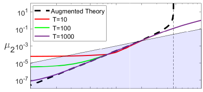
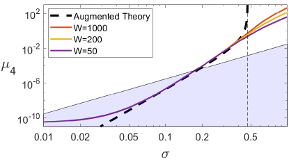
Figure 1: Numerical validation. Comparison of numerical results (via Fokker-Planck evolution) to the theoretical relation, augmented with the extra Gaussian condition $\mu_{4}=3\mu_{2}^{2}$. The shaded region indicates $\mu_{2}<0.1\sigma^{2}$ (top) and correspondingly $\mu_{4}<0.03\sigma^{4}$ (bottom), where the Gaussian approximation (from $\mu_{2}\ll\sigma^{2}$) should be most valid. Top: Smaller $\sigma$ values take longer simulated time $T$ to equilibrate, but do approach the theorized line in the shaded region. For high noise amplitudes, the relation need not hold, and indeed theory suggests that $\mu_{2}$ and $\mu_{4}$ should diverge for $\sigma>\sqrt{2}/3$ (indicated by the vertical dashed line)—though this divergence is invisible at constant domain width. Bottom: As predicted by theory, the fourth moment $\mu_{4}$ does indeed appear to diverge for $\sigma>\sqrt{2}/3$, though simulation with ever wider domain width $W$ (measured in number of standard deviations of the equilibrium solution) is needed capture more of the distribution’s tails (all curves shown for $T=100$).

I Conclusions

We have introduced an equilibrium-analysis technique for Itô SDEs inspired by the observation that such equilibria should theoretically be fixed under sufficiently precise numerical integration. The resulting analysis, which culminates in Eq. (5), should apply to any Itô system with an equilibrium where the second raw moment of that equilibrium is finite, but it is of particular use when the functions $F$ and $G^{2}$ are polynomial in nature, since this allows the analysis to yield explicit relations between even moments of the equilibrium rather than merely integrals against that unknown distribution.

We applied this technique to an example system arising from previous work, and were able to prove (by contradiction) that this system has a critical value of the noise parameter $\sigma$ at which its equilibrium must have divergent moments, since the relation becomes contradictory. This result would be very difficult to glean from direct numerical integration of the Itô (or corresponding Fokker-Planck) equation in question, due to the subtlety of this divergence in the distribution’s tails for any finite domain width.

In the analysis of this example system in the parameter region where its equilibrium has finite moments, we utilized an additional, near-Gaussian approximation (valid when $\mu_{2}\ll\sigma^{2}$) which allowed us to fully prescribe the moments of the equilibrium as a function of the noise parameter $\sigma$, and confirmed with numerical integration that the relation appears to hold—simulations converged to this augmented relation in the region of this approximation’s validity in forwards time. It remains unclear whether a more general constraint valid for arbitrary $\sigma$ closer to the moment-divergence boundary can be found. If such an additional constraint could be found and to the extent that it generalizes, this technique could enable the full specification of equilibrium moments. Regardless, we hope this analysis may yield some useful insight into specific systems which resist other techniques.

[width = 0.8color = black]88

See pages 1 of Sabin-Miller_SM_2.pdf

See pages 2 of Sabin-Miller_SM_2.pdf

See pages 3 of Sabin-Miller_SM_2.pdf