1 Introduction

Moving beyond $L^{p}$ geometric structure, Orlicz-Wasserstein (OW) leverages a specific class of convex functions for Orlicz geometric structure. Intuitively, OW is an instance of optimal transport (OT), which utilizes Orlicz metric as its ground cost (Sturm, 2011; Kell, 2017; Guha et al., 2023; Altschuler & Chewi, 2023; Le et al., 2024). Notably, OW remarkably helps to advance certain machine learning approaches. For examples, Altschuler & Chewi (2023) recently leverage OW as a metric shift for Rényi divergence and propose novel differential-privacy-inspired techniques to overcome longstanding challenges for proving fast convergence of hypocoercive differential equations. Additionally, Guha et al. (2023) leverage OW metric to alleviate several raised concerns caused from the usage of classical OT with Euclidean ground cost for quantifying the rates of parameter convergence within infinite Gaussian mixtures to significantly improve the Bayesian contraction rate of parameters arising from hierarchical Bayesian nonparametric models. However, OW has a high computational complexity steaming from its two-level optimization problem, i.e., one level for optimization plan, and the other level for an extra scalar in Orlicz metric structure. Recently, Le et al. (2024) propose generalized Sobolev transport, which is a scalable variant of OW for probability measures on a graph, for practical applications, especially for large-scale settings. Besides that, Orlicz geometric structure has been also applied for several machine learning problems, e.g., linear regression (Andoni et al., 2018; Song et al., 2019), scalable approaches for reinforcement learning, kernelized support vector machine, and clustering (Deng et al., 2022). Orlicz metric is also used to derive a finite-sample deviation bound for a general class of polynomial-growth functions to approximate high-order derivatives for arbitrary kernel (Chamakh et al., 2020), and as an OT regularization (Lorenz & Mahler, 2022).

When input measures have different total mass, several proposals have been developed in the literature (Hanin, 1992; Guittet, 2002; Benamou, 2003; Caffarelli & McCann, 2010; Figalli, 2010; Lellmann et al., 2014; Piccoli & Rossi, 2014, 2016; Frogner et al., 2015; Kondratyev et al., 2016; Liero et al., 2018; Chizat et al., 2018; Bonneel & Coeurjolly, 2019; Gangbo et al., 2019; Séjourné et al., 2019, 2022; Pham et al., 2020; Sato et al., 2020; Chapel et al., 2020; Balaji et al., 2020; Mukherjee et al., 2021; Le & Nguyen, 2021; Le et al., 2023; Nguyen et al., 2023), to name a few. The unbalanced setting for nonnegative measures has several applications, e.g., for color transfer and shape matching (Bonneel et al., 2015); multi-label learning (Frogner et al., 2015); positive-unlabeled learning (Chapel et al., 2020); natural language processing and topological data analysis (Le & Nguyen, 2021; Le et al., 2023); robust approaches for applications with noisy supports or outliers (Frogner et al., 2015; Balaji et al., 2020; Mukherjee et al., 2021).

In this work, we focus on OT problem with Orlicz geometric structure for unbalanced measures supported on a graph metric space (Le et al., 2022). Although GST (Le et al., 2023) provides a scalable variant for OW, GST assumes that input measures have the same mass as in OW. Unlike OT, it is nontrivial to incorporate a mass constraint to extend GST for general nonnegative measures on a graph. To address this challenge, our key insight is to take a step back to leverage Caffarelli & McCann (2010)’s observations, which allows to reformulate unbalanced optimal transport (UOT) problem as corresponding standard complete OT problem (Le et al., 2023), to propose Orlicz-EPT for unbalanced measures on a graph with Orlicz geometric structure. Furthermore, by exploiting the graph structure, we propose Orlicz-Sobolev transport, which scales Orlicz-EPT for practical applications.

Contribution. In summary, our contributions are two-fold as follows:

i) We propose to take a detour, and leverage EPT problem on a graph for unbalanced measures on a graph. By exploiting Caffarelli & McCann (2010)’s observations, we reformulate it as a corresponding standard complete OT to derive the proposed Orlicz-EPT. By further exploiting the graph structure, we develop a novel regularization and propose Orlicz-Sobolev transport (OST) which scales Orlicz-EPT for practical applications by showing that OST can be computed by solving a univariate optimization problem.

ii) We derive theoretical results for OST and draw its connections to other transport distances. We empirically illustrate that OST is several-order faster than Orlicz-EPT, and show preliminary evidences on the advantages of OST for document classification and topological data analysis.

Organization.

We briefly review related notions for our proposals in §2. In §3, we describe our proposed Orlicz-EPT and Orlicz-Sobolev transport (OST) based on EPT problem for unbalanced measures on a graph. Then, we derive theoretical properties for OST and draw its connections to other transport distances in §4. In §5, we discuss relations of the proposed approaches with other transport distances in the literature. We provide experimental results in §6, and conclude our work in §7.

2 Preliminaries

Graph. We use the same graph setting as in (Le et al., 2022). Specifically, let $V$ and $E$ be respectively the sets of nodes and edges. We consider a connected, undirected, and physical graph ${\mathbb{G}}=(V,E)$ with positive edge lengths $\{w_{e}\}_{e\in E}$. Following the convention in (Le et al., 2022) for continuous graph setting, ${\mathbb{G}}$ is regarded as the set of all nodes in $V$ together with all points forming the edges in $E$. Also, ${\mathbb{G}}$ is equipped with the graph metric $d_{{\mathbb{G}}}(x,y)$ which equals to the length of the shortest path in ${\mathbb{G}}$ between $x$ and $y$. Additionally, we assume that there exists a fixed root node $z_{0}\in V$ such that the shortest path connecting $z_{0}$ and $x$ is unique for any $x\in{\mathbb{G}}$, i.e., the uniqueness property of the shortest paths (Le et al., 2022).

Let $[x,z]$ denote the shortest path connecting $x$ and $z$ in ${\mathbb{G}}$. For $x\in{\mathbb{G}}$, edge $e\in E$, define the sets $\Lambda(x)$, $\gamma_{e}$ as follows:

$$\Lambda(x):=\big{\{}y\in{\mathbb{G}}:\,x\in[z_{0},y]\big{\}},$$

$$\gamma_{e}:=\big{\{}y\in{\mathbb{G}}:\,e\subset[z_{0},y]\big{\}}.$$ (1)

Denote ${\mathcal{P}}({\mathbb{G}})$ (resp.$\,{\mathcal{P}}({\mathbb{G}}\times{\mathbb{G}})$) as the set of all nonnegative Borel measures on ${\mathbb{G}}$ (resp.$\,{\mathbb{G}}\times{\mathbb{G}}$) with a finite mass.

Functions on graph. By a continuous function $f$ on ${\mathbb{G}}$, we mean that $f:{\mathbb{G}}\to\mathbb{R}$ is continuous w.r.t. the topology on ${\mathbb{G}}$ induced by the Euclidean distance. Henceforth, $C({\mathbb{G}})$ denotes the set of all continuous functions on ${\mathbb{G}}$. Similar notation is used for continuous functions on ${\mathbb{G}}\times{\mathbb{G}}$.

Given a scalar $b>0$, then a function $f:{\mathbb{G}}\to\mathbb{R}$ is called $b$-Lipschitz w.r.t. the graph metric $d_{\mathbb{G}}$ if

$$|f(x)-f(y)|\leq b\,d_{\mathbb{G}}(x,y),\,\,\forall x,y\in{\mathbb{G}}.$$

A family of convex functions. We consider the collection of $N$-functions (Adams & Fournier, 2003, §8.2) which are special convex functions on $\mathbb{R}_{+}$. Hereafter, a strictly increasing and convex function $\Phi:[0,\infty)\to[0,\infty)$ is called an $N$-function if $\lim_{t\to 0}\frac{\Phi(t)}{t}=0$ and $\lim_{t\to+\infty}\frac{\Phi(t)}{t}=+\infty$.

Orlicz functional space. Given an $N$-function $\Phi$ and a nonnegative Borel measure $\omega$ on ${\mathbb{G}}$, let $L_{\Phi}({\mathbb{G}},\omega)$ be the linear hull of the set of all Borel measurable functions $f:{\mathbb{G}}\to\mathbb{R}$ satisfying $\int_{{\mathbb{G}}}\Phi(|f(x)|)\omega(\text{d}x)<\infty$. Then, $L_{\Phi}({\mathbb{G}},\omega)$ is a normed space with the Luxemburg norm, defined as

$$\hskip-1.99997pt\left\lVert f\right\rVert_{L_{\Phi}}\!\coloneqq\!\inf\left\{t>0\mid\int_{{\mathbb{G}}}\Phi\left(\frac{|f(x)|}{t}\right)\omega(\text{d}x)\leq 1\right\}.$$ (2)

3 Orlicz-Sobolev Transport

In this section, for completeness, we briefly review the entropy partial transport (EPT) problem for unbalanced measures on a graph (Le et al., 2023, §3). We extend it for Orlicz geometric structure. Then, we describe our proposed Orlicz-Sobolev transport.

3.1 Orlicz-EPT: EPT on a Graph with Orlicz Structure

EPT on a graph.

Let $\gamma_{1},\gamma_{2}$ respectively be the first and second marginals of $\gamma\in{\mathcal{P}}({\mathbb{G}}\times{\mathbb{G}})$. For unbalanced measures $\mu,\nu\in{\mathcal{P}}({\mathbb{G}})$, we consider the set $\Pi_{\leq}(\mu,\nu):=\left\{\gamma:\,\gamma_{1}\leq\mu,\,\gamma_{2}\leq\nu\right\}$ where $\gamma_{1}\leq\mu$ means $\gamma_{1}(B)\leq\mu(B)$ for all Borel set $B\subset{\mathbb{G}}$, similarly for $\gamma_{2}\leq\nu$. Additionally, let $f_{1},f_{2}$ respectively be the Radon-Nikodym derivatives of $\gamma_{1}$ w.r.t. $\mu$ and of $\gamma_{2}$ w.r.t. $\nu$, i.e., $\gamma_{1}=f_{1}\mu$ ($0\leq f_{1}\leq 1$, $\mu$-a.e.) and $\gamma_{2}=f_{2}\nu$ ($0\leq f_{2}\leq 1$, $\nu$-a.e.).

For convex and lower semicontinuous entropy functions $F_{1},\,F_{2}:[0,1]\to(0,\infty)$, and nonnegative weight functions $w_{1},w_{2}:{\mathbb{G}}\to[0,\infty)$, we consider the weighted relative entropies of $\gamma_{1}$ w.r.t. $\mu$ and of $\gamma_{2}$ w.r.t. $\nu$ as follows:

$${\mathcal{F}}_{1}(\gamma_{1}|\mu) :=\int_{\mathbb{G}}w_{1}(x)F_{1}(f_{1}(x))\mu(\mathrm{d}x),$$ (3)

$${\mathcal{F}}_{2}(\gamma_{2}|\nu) :=\int_{\mathbb{G}}w_{2}(x)F_{2}(f_{2}(x))\nu(\mathrm{d}x).$$ (4)

We consider the graph metric $d_{{\mathbb{G}}}$ for the ground cost function. For a positive scalar $b>0$, and scalar $m\in[0,\bar{m}]$ where $\bar{m}:=\min\{\mu({\mathbb{G}}),\nu({\mathbb{G}})\}$, the EPT problem on ${\mathbb{G}}$ is

$$\hskip-1.00006pt\mathrm{W}_{m}(\mu,\nu):=\hskip-15.00002pt\inf_{\gamma\in\Pi_{\leq}(\mu,\nu),\,\gamma({\mathbb{G}}\times{\mathbb{G}})=m}\hskip-1.99997pt\Big{[}{\mathcal{F}}_{1}(\gamma_{1}|\mu)+{\mathcal{F}}_{2}(\gamma_{2}|\nu)+\,b\int_{{\mathbb{G}}\times{\mathbb{G}}}d_{{\mathbb{G}}}(x,y)\gamma(\mathrm{d}x,\mathrm{d}y)\Big{]}.\hskip 1.99997pt$$ (5)

As in Le et al. (2023, §3), by using the entropy functions $F_{1}(s)=F_{2}(s)=|s-1|$ and considering a Lagrange multiplier $\lambda\in\mathbb{R}$ conjugate to the constraint $\gamma({\mathbb{G}}\times{\mathbb{G}})=m$, we instead study the problem

$$\mathrm{ET}_{\lambda}(\mu,\nu)=\inf_{\gamma\in\Pi_{\leq}(\mu,\nu)}\mathcal{C}_{\lambda}(\gamma),$$ (6)

where $\mathcal{C}_{\lambda}(\gamma)=\int_{\mathbb{G}}\hskip-1.00006ptw_{1}\mu(\mathrm{d}x)+\int_{\mathbb{G}}\hskip-1.00006ptw_{2}\nu(\mathrm{d}x)-\int_{\mathbb{G}}\hskip-1.00006ptw_{1}\gamma_{1}(\mathrm{d}x)-\int_{\mathbb{G}}\hskip-1.00006ptw_{2}\gamma_{2}(\mathrm{d}x)+b\int_{{\mathbb{G}}\times{\mathbb{G}}}[d_{{\mathbb{G}}}(x,y)-\lambda]\gamma(\mathrm{d}x,\mathrm{d}y)$.

By leveraging the observation of Caffarelli & McCann (2010), we reformulate problem (6) as the standard complete OT problem. More specifically, we consider a point $\hat{s}$ outside graph ${\mathbb{G}}$ (i.e., $\hat{s}\notin{\mathbb{G}}$). We then extend the graph metric ground cost $d_{{\mathbb{G}}}$ to a new cost function $\hat{c}$ with $b\lambda$-deviation for its nonnegativity on the set $\hat{\mathbb{G}}:={\mathbb{G}}\cup\{\hat{s}\}$ as follows:

$$\hat{c}(x,y):=\left\{\begin{array}[]{lr}\!\!bd_{{\mathbb{G}}}(x,y)\hskip 28.99997pt\mbox{ if }x,y\in{\mathbb{G}},\\ \!\!w_{1}(x)+b\lambda\hskip 20.00003pt\mbox{ if }x\in{\mathbb{G}}\mbox{ and }y=\hat{s},\\ \!\!w_{2}(y)+b\lambda\hskip 20.00003pt\mbox{ if }x=\hat{s}\mbox{ and }y\in{\mathbb{G}},\\ \!\!b\lambda\hskip 57.00005pt\mbox{ if }x=y=\hat{s}.\end{array}\right.$$ (7)

For unbalanced measures $\mu,\nu$, by adding a Dirac mass at point $\hat{s}$, we construct corresponding balanced unit-mass measures $\hat{\mu}=\frac{\mu+\nu({\mathbb{G}})\delta_{\hat{s}}}{\mu({\mathbb{G}})+\nu({\mathbb{G}})}$ and $\hat{\nu}=\frac{\nu+\mu({\mathbb{G}})\delta_{\hat{s}}}{\mu({\mathbb{G}})+\nu({\mathbb{G}})}$. Consequently, we consider the standard complete OT problem between $\hat{\mu},\hat{\nu}$ with cost $\hat{c}$ as follows

$$\mathrm{KT}(\mu,\nu):=\left(\mu({\mathbb{G}})+\nu({\mathbb{G}})\right)\left(\mathcal{W}_{\hat{c}}(\hat{\mu},\hat{\nu})-b\lambda\right),$$ (8)

where $\mathcal{W}_{\hat{c}}(\hat{\mu},\hat{\nu}):=\inf_{\tilde{\gamma}\in\Pi(\hat{\mu},\hat{\nu})}\int_{\hat{\mathbb{G}}\times\hat{\mathbb{G}}}\hat{c}(x,y)\tilde{\gamma}(\mathrm{d}x,\mathrm{d}y)$, and $\Pi(\hat{\mu},\hat{\nu}):=\Big{\{}\hat{\gamma}\in{\mathcal{P}}(\hat{\mathbb{G}}\times\hat{\mathbb{G}}):\hat{\mu}(U)=\hat{\gamma}(U\times\hat{\mathbb{G}}),\,\hat{\nu}(U)=\hat{\gamma}(\hat{\mathbb{G}}\times U)\mbox{ for all Borel sets }U\subset\hat{\mathbb{G}}\Big{\}}$.

Therefore, one can reformulate an unbalanced OT problem (6) into a corresponding standard complete OT (8). Consequently, we not only bypass all the technical challenges in the unbalanced setting but also utilize abundant existing results and approaches in the standard balanced setting for OT problem with unbalanced measures on a graph.

Remark 3.1 (Nonnegativity).

The nonnegativity of the cost function $\hat{c}$ (7) for standard OT (6) is essential for the development of EPT with Orlicz geometric structure. We remark that such nonnegativity is not guaranteed in Le et al. (2023).

Orlicz-EPT.

Following the approaches in Sturm (2011); Kell (2017); Guha et al. (2023); Chewi (2023), we define Orlicz-EPT, i.e., EPT with Orlicz geometric structure, upon the corresponding standard OT problem (8) as follows:

$$\mathcal{OE}_{\Phi}(\mu,\nu):=\left(\mu({\mathbb{G}})+\nu({\mathbb{G}})\right)(\mathcal{W}_{\Phi}(\hat{\mu},\hat{\nu})-b\lambda),$$ (9)

where $\mathcal{W}_{\Phi}(\hat{\mu},\hat{\nu}):=\inf_{\tilde{\gamma}\in\Pi(\hat{\mu},\hat{\nu})}\inf\Big{[}t>0:\int_{\hat{\mathbb{G}}\times\hat{\mathbb{G}}}\Phi\left(\frac{\hat{c}(x,y)}{t}\right)\text{d}\tilde{\gamma}(x,y)\leq 1\Big{]}$.

We next show that the objective function of Orlicz-EPT w.r.t. $t$ is monotonically non-increasing.

Proposition 3.2 (Monotonicity).

For unbalanced measures $\mu,\nu\in{\mathcal{P}}({\mathbb{G}})$, construct corresponding $\hat{\mu},\hat{\nu},\hat{c}$. For an $N$-function $\Phi$, let

$$\mathcal{A}(t;\hat{\mu},\hat{\nu}):=\inf_{\tilde{\gamma}\in\Pi(\hat{\mu},\hat{\nu})}\int_{\hat{\mathbb{G}}\times\hat{\mathbb{G}}}\Phi\left(\frac{\hat{c}(x,y)}{t}\right)\mathrm{d}\tilde{\gamma}(x,y).$$ (10)

Then, $\mathcal{A}(t;\hat{\mu},\hat{\nu})$ is monotonically non-increasing w.r.t. $t$.

Proof is placed in Appendix §A.1.

Computation.

Observe that for a fixed $t$, $\mathcal{A}$ is a standard OT problem between $\hat{\mu}$ and $\hat{\nu}$ with the cost function $\Phi\!\left(\frac{\hat{c}(\cdot,\cdot)}{t}\right)$. We show that the monotonicity is preserved for its corresponding entropic regularization.

Proposition 3.3 (Entropic regularization).

Define the entropic regularization of $\mathcal{A}$ as

$$\mathcal{A}_{\varepsilon}(t;\hat{\mu},\hat{\nu})\!:=\!\hskip-10.00002pt\inf_{\tilde{\gamma}\in\Pi(\hat{\mu},\hat{\nu})}\hskip-1.00006pt\!\left[\int_{\hat{\mathbb{G}}\times\hat{\mathbb{G}}}\hskip-11.99998pt\Phi\left(\!\frac{\hat{c}(x,y)}{t}\!\right)\!\mathrm{d}\tilde{\gamma}(x,y)\!-\!\varepsilon H(\tilde{\gamma})\right],$$ (11)

where $\varepsilon\geq 0$ and $H$ is Shannon entropy defined as $H(\tilde{\gamma}):=-\int_{\hat{\mathbb{G}}\times\hat{\mathbb{G}}}(\log\tilde{\gamma}(x,y)-1)\mathrm{d}\tilde{\gamma}(x,y)$. Then, $\mathcal{A}_{\varepsilon}(t;\hat{\mu},\hat{\nu})$ is monotonically non-increasing w.r.t. $t$.

Proof is placed in Appendix §A.2.

Additionally, we derive the upper and lower bounds for $\mathcal{A}_{\varepsilon}$.

Proposition 3.4 (Bounds).

We have

$$\hskip-5.0pt\mathcal{A}_{\varepsilon}\!\left(\frac{\mathcal{W}_{\hat{c}}(\hat{\mu},\hat{\nu})}{\Phi^{-1}(1+\varepsilon\left[H(\hat{\mu})+H(\hat{\nu})-1\right])};\hat{\mu},\hat{\nu}\right)\geq 1,$$

$$\mathcal{A}_{\varepsilon}\!\left(\frac{L_{\hat{\mu},\hat{\nu}}}{\Phi^{-1}(1+\varepsilon)};\hat{\mu},\hat{\nu}\right)\leq 1,$$

where $L_{\hat{\mu},\hat{\nu}}=\max_{x\in\mathrm{supp}(\hat{\mu}),y\in\mathrm{supp}(\hat{\nu})}\hat{c}(x,y)$, and $\mathrm{supp}(\cdot)$ is a set of supports of a measure.

Proof is placed in Appendix §A.3.

From the monotonicity of $\mathcal{A}_{\varepsilon}$ in Proposition 3.3, and the limits of $\mathcal{A}_{\varepsilon}$ in Proposition 3.4, we can leverage the binary search to compute the entropic regularized Orlicz-EPT (corresponding to the original Orlicz-EPT (9)), defined as:

$$\mathcal{OE}_{\Phi,\varepsilon}(\mu,\nu):=\left(\mu({\mathbb{G}})+\nu({\mathbb{G}})\right)(\mathcal{W}_{\Phi,\varepsilon}(\hat{\mu},\hat{\nu})-b\lambda),$$ (12)

where $\mathcal{W}_{\Phi,\varepsilon}(\hat{\mu},\hat{\nu}):=\inf_{\tilde{\gamma}\in\Pi(\hat{\mu},\hat{\nu})}\inf\Big{[}t>0:\int_{\hat{\mathbb{G}}\times\hat{\mathbb{G}}}\Phi\left(\frac{\hat{c}(x,y)}{t}\right)\text{d}\tilde{\gamma}(x,y)-\varepsilon H(\tilde{\gamma})\leq 1\Big{]}$.

Although the entropic regularized Orlicz-EPT $\mathcal{OE}_{\Phi,\varepsilon}$ (12) scales up the computation of the original Orlicz-EPT $\mathcal{OE}_{\Phi}$ (9) by leveraging binary search on the quadratic-complexity $\mathcal{A}_{\varepsilon}$ (11) instead of the super-cubic-complexity $\mathcal{A}$ (10), the nature two-level optimization complexity of $\mathcal{OE}_{\Phi,\varepsilon}$ still remains, which hinders its practical applications, especially in large-scale settings. To tackle this computational challenge, we next leverage a collection of special convex functions (i.e., $N$-functions) to propose the Orlicz-Sobolev transport, which can adopt Orlicz geometric structure in the same sense as the Orlicz-EPT, and especially, it is much more efficient for computation.

3.2 Orlicz-Sobolev Transport

We recall the dual formula of EPT, and the graph-based Orlicz-Sobolev space which play as the key components for our proposed Orlicz-Sobolev transport (OST) for unbalanced measures on a graph.

Dual formula of EPT on a graph (Le et al., 2023).

Assume that $\lambda\geq 0$ and the nonnegative weight functions $w_{1},w_{2}$ are $b$-Lipschitz w.r.t. $d_{\mathbb{G}}$. Following Le et al. (2023, Corollary 3.2), the dual EPT on a graph is as follows:

$$\mathrm{ET}_{\lambda}(\mu,\nu)=\sup_{f\in\mathbb{U}}\int_{\mathbb{G}}f(\mu-\nu)-\frac{b\lambda}{2}\big{[}\mu({\mathbb{G}})+\nu({\mathbb{G}})\big{]},$$ (13)

where $\mathbb{U}:=\big{\{}f\in C({\mathbb{G}}):-w_{2}-\frac{b\lambda}{2}\leq f\leq w_{1}+\frac{b\lambda}{2},\,|f(x)-f(y)|\leq b\,d_{\mathbb{G}}(x,y)\big{\}}$.

Graph-based Orlicz-Sobolev space (Le et al., 2024).

Let $\Phi$ be an $N$-function and $\omega$ be a nonnegative Borel measure on graph ${\mathbb{G}}$. A continuous function $f:{\mathbb{G}}\to\mathbb{R}$ is said to belong to the graph-based Orlicz-Sobolev space $W\!L_{\Phi}({\mathbb{G}},\omega)$ if there exists a function $h\in L_{\Phi}({\mathbb{G}},\omega)$ satisfying

$$f(x)-f(z_{0})=\int_{[z_{0},x]}h(y)\omega(\mathrm{d}y),\quad\forall x\in{\mathbb{G}}.$$ (14)

Such function $h$ is unique in $L_{\Phi}({\mathbb{G}},\omega)$ and is called the generalized graph derivative of $f$ w.r.t. the measure $\omega$. Henceforth, this generalized graph derivative of $f$ is denoted $f^{\prime}$.

Orlicz-Sobolev transport (OST).

Inspired by the generalized Sobolev transport (Le et al., 2024), we exploit the dual EPT on a graph. We then replace the Lipschitz constraint for the critic function $f$ in $\mathbb{U}$ by a constraint involving the graph-based Orlicz-Sobolev space, i.e., $f\in W\!L_{\Psi}({\mathbb{G}},\omega),\left\lVert f^{\prime}\right\rVert_{L_{\Psi}}\leq b$ where $\Psi$ is the complement $N$-function of $\Phi$. Moreover, thanks to the observation in Le & Nguyen (2021), from Equation (14) and $\left\lVert f^{\prime}\right\rVert_{L_{\Psi}}\leq b$, we employ the generalized Hölder inequality w.r.t. Luxemburg norm in Orlicz space $L_{\Psi}({\mathbb{G}},\omega)$ (Adams & Fournier, 2003, §8.11), then $\int_{[z_{0},x]}f^{\prime}(y)\omega(\mathrm{d}y)$ is controlled by $2b/\Phi^{-1}\!\left(\omega([z_{0},x])^{-1}\right)$. Therefore, instead of the bounded constraint on the critic function $f$ in $\mathbb{U}$, we constraint only on $f(z_{0})$.

Definition 3.5 (Orlicz-Sobolev transport).

Let $\omega$ be a nonnegative Borel measure on graph ${\mathbb{G}}$, and ${\mathcal{I}}_{\alpha}:=\left[-w_{2}(z_{0})-\frac{b\lambda}{2}+\alpha,w_{1}(z_{0})+\frac{b\lambda}{2}-\alpha\right]$ where $\alpha\in[0,\frac{1}{2}(b\lambda+w_{1}(z_{0})+w_{2}(z_{0}))]$. Given a pair of complementary $N$-functions $\Phi,\Psi$, and for $\mu,\nu\in{\mathcal{P}}({\mathbb{G}})$, the Orlicz-Sobolev transport is defined as follows

$$\mathcal{OS}_{\Phi,\alpha}(\mu,\nu)\hskip-1.99997pt:=\hskip-6.00006pt\sup_{f\in\mathbb{U}_{\Psi,\alpha}}\hskip-3.00003pt\left[\int_{\mathbb{G}}\hskip-3.99994ptf(x)\mu(\mathrm{d}x)-\int_{\mathbb{G}}\hskip-3.99994ptf(x)\nu(\mathrm{d}x)\right]\!,$$ (15)

where $\mathbb{U}_{\Psi,\alpha}\!:=\!\big{\{}f\!\in\!W\!L_{\Psi}({\mathbb{G}},\omega),\left\lVert f^{\prime}\right\rVert_{L_{\Psi}}\!\leq\!b,f(z_{0})\!\in\!{\mathcal{I}}_{\alpha}\big{\}}$.

Intuitively, $\mathbb{U}_{\Psi,\alpha}$ is the collection of all functions $f$, expressed by $f(x)=s+\int_{[z_{0},x]}h(y)\omega(\mathrm{d}y),\forall x\in{\mathbb{G}}$, where $s\in{\mathcal{I}}_{\alpha}$, and $\left\lVert h\right\rVert_{L_{\Psi}}\leq b$. The upper bound constraint on $\alpha$ is to ensure that ${\mathcal{I}}_{\alpha}$ is nonempty. When $\alpha=0$, the interval ${\mathcal{I}}_{\alpha}$ is the largest. Additionally, OST for unbalanced measures on a graph is an instance of the integral probability metric (Müller, 1997).

Computation.

We show that OST can be efficiently computed by simply solving a corresponding univariate optimization problem.

Theorem 3.6 (OST as a univariate optimization problem).

Given two unbalanced measures $\mu,\nu\in{\mathcal{P}}({\mathbb{G}})$, define

$$\Theta:=\left\{\begin{array}[]{lr}w_{1}(z_{0})+\frac{b\lambda}{2}-\alpha&\mbox{if}\quad\mu({\mathbb{G}})\geq\nu({\mathbb{G}}),\\ w_{2}(z_{0})+\frac{b\lambda}{2}-\alpha&\mbox{if}\quad\mu({\mathbb{G}})<\nu({\mathbb{G}}).\end{array}\right.$$ (18)

Then, Orlicz-Sobolev transport can be computed as follows:

$$\mathcal{OS}_{\Phi,\alpha}(\mu,\nu)=\Theta|\mu({\mathbb{G}})-\nu({\mathbb{G}})|+\inf_{k>0}\frac{1}{k}\left(1+\hskip-3.00003pt\int_{{\mathbb{G}}}\hskip-3.00003pt\Phi\left(kb\left|\mu(\Lambda(x))-\nu(\Lambda(x))\right|\right)\omega(\text{d}x)\right)\!.$$ (19)

The proof is placed in Appendix §A.4.

We next derive the discrete case for the OST. Especially, we provide an explicit expression for the integral in Equation (14).

Corollary 3.7 (Discrete case).

Let $\omega$ be the length measure of graph ${\mathbb{G}}$, and input measures $\mu,\nu$ are supported on nodes in $V$ of graph ${\mathbb{G}}$. Then, we have

$$\mathcal{OS}_{\Phi,\alpha}(\mu,\nu)=\Theta|\mu({\mathbb{G}})-\nu({\mathbb{G}})|+\inf_{k>0}\frac{1}{k}\left(1+\hskip-3.00003pt\sum_{e\in E}\hskip-1.00006ptw_{e}\Phi\!\left(kb\left|\mu(\gamma_{e})-\nu(\gamma_{e})\right|\right)\right),$$ (20)

The proof is placed in Appendix §A.5.

Therefore, the OST (Definition 3.5) can be efficiently computed by simply solving the univariate optimization problem (20) (e.g., by second-order methods).

Remark 3.8 (Non-physical graph).

Although ${\mathbb{G}}$ is assumed to be a physical graph (§2), Corollary 3.7 implies that OST only depends on the graph structure $(V,E)$ and edge weights $w_{e}$ when measures are supported on nodes in $V$ of graph ${\mathbb{G}}$, i.e., OST is applicable for non-physical graph ${\mathbb{G}}$.

Remark 3.9 (Complementary pairs of $N$-functions).

Corollary 3.7 also implies that one can compute OST with $N$-function $\Phi$ without involving its complementary $N$-function $\Psi$ (Equation (20)), unlike its definition (Equation (15)). It requires that $\Psi$ is finited-value to derive the univariate optimization formula (20)), which is satisfied for any $N$-function $\Phi$, i.e., growing faster than linear.

Preprocessing for $\gamma_{e}$. Following the observation in Le et al. (2024), we precompute set $\gamma_{e}$ (Equation (2)) for all edge $e$ in ${\mathbb{G}}$. More concretely, we apply the Dijkstra algorithm to recompute the shortest paths from the root node $z_{0}$ to all other vertices in $V$ with complexity $\mathcal{O}(|E|+|V|\log{|V|})$, where $|\cdot|$ is the set cardinality.

Remark 3.10 (Sparsity).

Observe that $\forall x\in\text{supp}(\mu)$, its mass is gathered into $\mu(\gamma_{e})$ if and only if $e\subset[z_{0},x]$ (Le et al., 2024). Therefore, by defining set $E_{\mu,\nu}\subset E$ as

$$E_{\mu,\nu}\hskip-1.99997pt:=\hskip-1.99997pt\left\{e\!\in\!E\mid\exists z\!\in\!(\text{supp}(\mu)\cup\text{supp}(\nu)),e\subset[z_{0},z]\right\}\!,$$

it suffices to compute the summation only over edges $e\in E_{\mu,\nu}$ in Equation (20) for OST, i.e., screening all edges $e\in E\setminus E_{\mu,\nu}$.

4 Theoretical Properties

Orlicz-EPT has its own interesting characteristics. However, it has a high computational complexity due to its two-level optimization formula, which hinders its practical applications. Thus, in this section, we mainly focus on theoretical properties for Orlicz-Sobolev transport (OST).

4.1 Geometric Structure of Orlicz-Sobolev Transport

We derive the geometric structure of OST. Under certain conditions, we prove that OST is a metric.

Proposition 4.1 (Geometric structures of OST).

Let $\omega$ be a nonnegative Borel measure on graph ${\mathbb{G}}$. Assume that $\lambda,w_{1}(z_{0}),w_{2}(z_{0})\geq 0$, and $0\leq\alpha<\frac{b\lambda}{2}+\min\{w_{1}(z_{0}),w_{2}(z_{0})\}$. Then, $\forall\mu,\nu,\sigma\in{\mathcal{P}}({\mathbb{G}})$, we have

i) $\mathcal{OS}_{\Phi,\alpha}(\mu+\sigma,\nu+\sigma)=\mathcal{OS}_{\Phi,\alpha}(\mu,\nu)$.

ii) $\mathcal{OS}_{\Phi,\alpha}$ is a divergence. It also satisfies the triangle inequality: $\mathcal{OS}_{\Phi,\alpha}(\mu,\nu)\leq\mathcal{OS}_{\Phi,\alpha}(\mu,\sigma)+\mathcal{OS}_{\Phi,\alpha}(\sigma,\nu)$.

iii) With an additional assumption $w_{1}(z_{0})=w_{2}(z_{0})$, then $\mathcal{OS}_{\Phi,\alpha}$ is a metric.

The proof is placed in Appendix §A.6.

4.2 Relations to Other Transport Distances

We draw several connections for OST with other transport distances on graph ${\mathbb{G}}$, including generalized Sobolev transport (GST) (Le et al., 2024), Sobolev transport (ST) (Le et al., 2022), unbalanced Sobolev transport (UST) (Le et al., 2023), Orlicz-EPT (§3.1), a variant of regularized EPT (Le & Nguyen, 2021), and standard optimal transport (OT). Additionally, we consider the limit case $\Phi(t)=t$ for $N$-function, and the special case when graph ${\mathbb{G}}$ is a tree.

Connection with generalized Sobolev transport.

Proposition 4.2.

Assume that $\mu({\mathbb{G}})=\nu({\mathbb{G}})$, $b=1$, and denote $\mathcal{GS}_{\Phi}$ for the GST with $N$-function $\Phi$, then we have

$$\mathcal{OS}_{\Phi,\alpha}(\mu,\nu)=\mathcal{GS}_{\Phi}(\mu,\nu).$$

The proof is placed in Appendix §A.7.

Connection with Sobolev transport.

Proposition 4.3.

Assume that $\mu({\mathbb{G}})=\nu({\mathbb{G}})$, $b=1$, and denote $\mathcal{S}_{p}$ for the $p$-order Sobolev transport. Then, for $1<p<\infty$ and $N$-function $\Phi(t)=\frac{(p-1)^{p-1}}{p^{p}}t^{p}$, we have

$$\mathcal{OS}_{\Phi,\alpha}(\mu,\nu)=\mathcal{S}_{p}(\mu,\nu).$$

The proof is placed in Appendix §A.8.

Connection with unbalanced Sobolev transport.

Proposition 4.4.

For $N$-function $\Phi(t)=\frac{(p-1)^{p-1}}{p^{p}}t^{p}$ with $1<p<\infty$, and denote $\mathcal{US}_{p,\alpha}$ for the unbalanced Sobolev transport, then we have

$$\mathcal{OS}_{\Phi,\alpha}(\mu,\nu)=\mathcal{US}_{p,\alpha}(\mu,\nu).$$

The proof is placed in Appendix §A.9.

For the limit case: $\Phi(t)=t$

.

Proposition 4.5 (Limit case for OST).

For $\Phi(t)=t$, and with the same assumptions in Corollary 3.7, then OST yields a closed-form expression as follows:

$$\hskip-3.00003pt\mathcal{OS}_{\Phi,\alpha}(\mu,\nu)\!=\!b\!\sum_{e\in E}\hskip-1.00006ptw_{e}\!\left|\mu(\gamma_{e})\!-\!\nu(\gamma_{e})\right|\!+\!\Theta|\mu({\mathbb{G}})\!-\!\nu({\mathbb{G}})|.$$ (21)

Moreover, it is equal to the $1$-order unbalanced Sobolev transport (Le et al., 2023).

The proof is placed in Appendix §A.10.

Proposition 4.6 (Limit case for Orlicz-EPT).

For $\Phi(t)=t$, and $\mu,\nu\in{\mathcal{P}}({\mathbb{G}})$, then Orlicz-EPT is equal to EPT on a graph (Le et al., 2023), i.e.,

$$\mathcal{OE}_{\Phi}(\mu,\nu)=\mathrm{KT}(\mu,\nu).$$ (22)

The proof is placed in Appendix §A.11.

Proposition 4.7 (Relation of OST and Orlicz-EPT).

Assume that $\Phi(t)=t$, $\omega$ is the length measure on ${\mathbb{G}}$, $\lambda\geq 0$, nonnegative weight functions $w_{1},w_{2}$ are $b$-Lipschitz w.r.t. $d_{{\mathbb{G}}}$, $\alpha=0$, $p=1$. Then we have

$$\mathcal{OS}_{\Phi,\alpha}(\mu,\nu)\geq\mathcal{OE}_{\Phi}(\mu,\nu)+\frac{b\lambda}{2}(\mu({\mathbb{G}})+\nu({\mathbb{G}})).$$

The proof is placed in Appendix §A.12.

For the special cases when graph ${\mathbb{G}}$ is a tree.

Proposition 4.8 (Relation of OST and a variant of regularized EPT).

Under the same assumptions as in Proposition 4.5, and assume in addition that graph ${\mathbb{G}}$ is a tree, then we have

$$\mathcal{OS}_{\Phi,\alpha}(\mu,\nu)=d_{\alpha}(\mu,\nu),$$

where $d_{\alpha}$ is a variant of the regularized EPT, defined in Le & Nguyen (2021, Equation (9)).

The proof is placed in Appendix §A.13.

Proposition 4.9 (Relation of OST and OT).

Under the same assumptions as in Proposition 4.8, and assume in addition that $\mu({\mathbb{G}})=\nu({\mathbb{G}})$ and $b=1$, then we have

$$\mathcal{OS}_{\Phi,\alpha}(\mu,\nu)=\mathcal{W}_{d_{{\mathbb{G}}}}(\mu,\nu),$$

where $\mathcal{W}_{d_{{\mathbb{G}}}}$ is the standard optimal transport with graph metric ground cost $d_{{\mathbb{G}}}$.

The proof is placed in Appendix §A.14.

5 Related Works and Discussions

The proposed Orlicz-Sobolev transport (OST) generalizes GST (Le et al., 2024) for unbalanced measures supported on a graph (see Proposition 4.2). We emphasize that unlike OT, it is nontrivial to incorporate mass constraints for GST, since as its root, the definition of GST is steamed from the Kantorovich duality of $1$-order Wasserstein, and it optimizes the critic function with constraints in the graph-based Orlicz-Sobolev space. Therefore, it is essential to take a detour to consider EPT problem for unbalanced measures on a graph (Le et al., 2023), then leverage Caffarelli & McCann (2010)’s observations to derive a corresponding standard complete OT problem, and incorporate back the Orlicz geometric structure for the proposed Orlicz-EPT. We further note that Caffarelli & McCann (2010)’s observations may not be applicable for some other certain formulations of unbalanced optimal transport (UOT) such as those in Frogner et al. (2015); Chizat et al. (2018); Séjourné et al. (2019).

Moreover, Orlicz-EPT is formulated as a two-level optimization problem (Equation (9)) which leads to a high-computational cost and hinders its practical applications, similar to OW for the case of balanced measures. By leveraging Le & Nguyen (2021)’s observations and exploiting graph structure, we propose novel regularization for critic function within the Orlicz-Sobolev space, and develop OST. Our key result is to show that one can simply solving a univariate optimization problem (Theorem 3.6) for OST computation, and make it more practical for applications.

6 Experiments

In this section, we illustrate that the computation of Orlicz-EPT with $N$-function $\Phi$ is very costly. Especially, the Orlicz-Sobolev transport (OST) is several-order faster than Orlicz-EPT. Following the setup simulations in Le et al. (2023), we evaluate OST for unbalanced measures supported a given graph, and show preliminary evidences on its advantages for document classification and TDA.

Document classification. Following Le et al. (2023), we use four document datasets: TWITTER, RECIPE, CLASSIC, and AMAZON. We summarize these dataset characteristics in Figure 5. By regarding each word in a document as a support with a unit mass, we represent each document as a nonnegative measure. Consequently, the representations of documents with different lengths are measures with different total mass. We apply the same word embedding procedure in Le et al. (2023) to map words into vectors in $\mathbb{R}^{300}$ (i.e., word2vec (Mikolov et al., 2013) pretrained on Google News).

Table 1: The number of pairs for SVM.

Datasets	#pairs
TWITTER	4394432
RECIPE	8687560
CLASSIC	22890777
AMAZON	29117200
Orbit	11373250
MPEG7	18130

TDA. As in Le et al. (2023), we consider orbit recognition on Orbit dataset (Adams et al., 2017), and object shape classification on MPEG7 dataset (Latecki et al., 2000). We summarize these dataset characteristics in Figure 6. We use persistence diagrams (PD) to represent objects of interest. We then consider each $2$-dimensional data point in PD as a support with a unit-mass, and represent PD as nonnegative measures. As a result, PD having different numbers of topological features are presented as measures with different total mass.

Graph. Following Le et al. (2023), we use the graphs ${\mathbb{G}}_{\text{Log}}$ and ${\mathbb{G}}_{\text{Sqrt}}$ (Le et al., 2022, §5) for our simulations, which empirically satisfy the assumptions in §2. Additionally, we set $M=10^{4}$ for the number of nodes for these graphs, except experiments on MPEG7 dataset with $M=10^{3}$ due to its small size.

$N$-function. Following Le et al. (2024), we consider two $N$-functions: $\Phi_{1}(t)=\exp(t)-t-1$, and $\Phi_{2}(t)=\exp(t^{2})-1$, and the limit case: $\Phi_{0}(t)=t$.

Parameters. For simplicity, we follow the same setup as in Le et al. (2023). We set $\lambda=b=1$, $\alpha=0$, and consider the weight functions $w_{1}(x)\!=\!w_{2}(x)\!=\!a_{1}d_{{\mathbb{G}}}(z_{0},x)+a_{0}$ where $a_{1}\!=\!b$ and $a_{0}\!=\!1$. The entropic regularization $\varepsilon$ is chosen $\left\{0.01,0.1,1,10\right\}$, e.g., via cross validation.

Optimization algorithm. For OST computation, we apply a second-order method, e.g., fmincon Trust Region Reflective solver in MATLAB, for solving the univariate optimization problem.

SVM classification. For document classification and TDA, we use support vector machine (SVM) with kernels $\exp(-\bar{t}\bar{d}(\cdot,\cdot))$, where $\bar{d}$ is a distance/discrepancy (e.g., OST, Orlicz-EPT) for unbalanced measures supported on a graph, and $\bar{t}>0$. Additionally, following Cuturi (2013), we regularize Gram matrices by adding a sufficiently large diagonal term for indefinite kernels. In Table 1, we summarize the number of pairs which we need to evaluate distances/discrepancies for SVM in each run to illustrate the experimental scale.

Set up. We randomly split each dataset into $70\%/30\%$ for training and test, and use $10$ repeats. Basically, we choose hyper-parameters via cross validation. More concretely, we choose kernel hyperparameter from $\{1/q_{s},0.5/q_{s},0.2/q_{s}\}$ with $s=10,20,\dotsc,90$, where $q_{s}$ is the $s\%$ quantile of a subset of distances observed on a training set; SVM regularization hyperparameter from $\left\{0.01,0.1,1,10\right\}$; root node $z_{0}$ from a random $10$-root-node subset of $V$ in graph ${\mathbb{G}}$. We note that reported time consumption includes all preprocessing procedures, e.g., preprocessing for $\gamma_{e}$ for OST.

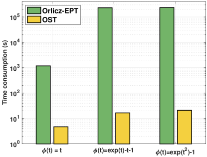
Figure 1: Time consumption on graph ${\mathbb{G}}_{\text{Sqrt}}$.

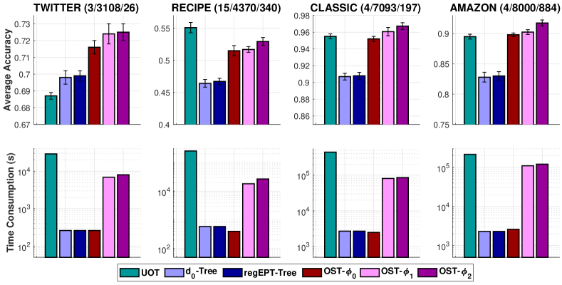
Figure 2: Document classification on graph ${\mathbb{G}}_{\text{Sqrt}}$. For each dataset, the numbers in the parenthesis are respectively the number of classes; the number of documents; and the maximum number of unique words for each document.

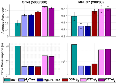
Figure 3: TDA on graph ${\mathbb{G}}_{\text{Sqrt}}$. For each dataset, the numbers in the parenthesis are respectively the number of PD; and the maximum number of points in PD.

6.1 Computation

We compare the time consumption of OST and Orlicz-EPT with $N$-functions $\Phi_{1},\Phi_{2}$, and the limit case $\Phi_{0}$.

Set up. We randomly sample $10^{4}$ pairs of nonnegative measures on AMAZON dataset for evaluation. We $M=10^{3}$ for graphs, and $\varepsilon=0.1$ for Orlicz-EPT.

Results. In Figure 1, we illustrate the time consumptions on ${\mathbb{G}}_{\text{Sqrt}}$. OST is several-order faster than Orlicz-EPT, i.e., at least $250\times,13800\times,11200\times$ for $\Phi_{0},\Phi_{1},\Phi_{2}$ respectively. Notably, for $N$-functions $\Phi_{1},\Phi_{2}$, Orlicz-EPT takes at least $2.6$ days, while OST takes less than $21$ seconds. Note that for the limit case $\Phi_{0}$, Orlicz-EPT is equal to EPT on a graph (Proposition 4.6), and OST admits a closed-form expression (Proposition 4.5). Consequently, Orlicz-EPT and OST with $\Phi_{0}$ is more computationally efficient than those with $\Phi_{1},\Phi_{2}$.

6.2 Document classification

Set up. We carry out OST with $\Phi_{0},\Phi_{1},\Phi_{2}$ (§6.1), and denote them as OST-$\Phi_{i}$ for $i=0,1,2$. We exclude Orlicz-EPT due to their heavy computations (§6.1). Additionally, following Le et al. (2023), we consider unbalanced optimal transport (UOT) (Frogner et al., 2015; Séjourné et al., 2019) with ground cost $d_{{\mathbb{G}}}$, and special cases with tree-structure graph. More concretely, we randomly sample a tree from the given graph ${\mathbb{G}}$, then consider the regularized EPT and $d_{0}$, denoted as $d_{0}$-Tree and regEPT-Tree, for unbalanced measures with the sampled tree (Le & Nguyen, 2021, Proposition 3.8, and Equation (9) respectively).

Results. In Figure 2, we show SVM results and time consumptions of kernels on graph ${\mathbb{G}}_{\text{Sqrt}}$. The performances of OST with all $\Phi$ functions are comparable to UOT, but the computation of UOT is more costly than OST. Additionally, OST outperforms $d_{0}$-Tree and regEPT-Tree. However, the computations of OST-$\Phi_{1}$, OST-$\Phi_{2}$ are more expensive while the computation of OST-$\Phi_{0}$ is comparative to those fast-computational variants of UOT on tree (i.e., $d_{0}$-Tree and regEPT-Tree). Moreover, OST-$\Phi_{1}$ and OST-$\Phi_{2}$ improve performances of OST-$\Phi_{0}$, but their computational time is several-order higher. It may imply that Orlicz geometric structure in OST may be helpful for document classification. UOT performs well on RECIPE, but worse on TWITTER which agrees with observations in Le et al. (2023).

6.3 Topological Data Analysis

Set up. Similarly, we also evaluate OST-$\Phi_{0}$, OST-$\Phi_{1}$, OST-$\Phi_{2}$, UOT, $d_{0}$-Tree, and regEPT-Tree for TDA.

Results. In Figure 3, we illustrate SVM results and time consumptions of kernels on graph ${\mathbb{G}}_{\text{Sqrt}}$. Performances of OST with all $\Phi$ functions compare favorably with other transport distance approaches. Especially, performances of OST-$\Phi_{1}$ and OST-$\Phi_{2}$ compare favorably with those of OST-$\Phi_{0}$, but it comes with higher computational cost (i.e., OST-$\Phi_{0}$ has a closed-form expression for a fast computation (Proposition 4.5)). Therefore, Orlicz geometric structure is also helpful for TDA.

7 Conclusion

In this work, we propose novel approaches to extend generalized Sobolev transport, i.e., a scalable variant of Orlicz-Wasserstein, for nonnegative measures on a graph. More specifically, based on entropy partial transport (EPT) for unbalanced measures, we leverage Caffarelli & McCann (2010)’s observations to develop Orlicz-EPT. Furthermore, by exploiting a special family of convex functions (i.e., the set of $N$-functions) and geometric structure of the graph-based Orlicz-Sobolev space, we propose Orlicz-Sobolev transport (OST) with efficient computation. Note that it suffices to compute OST by simply solving a univariate optimization problem while one needs to solve a complex two-level optimization problem to compute Orlicz-EPT.

Impact Statement

The paper proposes novel approaches for optimal transport problem with Orlicz geometric structure for unbalanced measures on a graph. Especially, our proposed Orlicz-Sobolev transport can be computed efficiently by simply solving a univariate optimization problem, which paves a way for its usages in practical applications, especially for large-scale settings. To our knowledge, there are no foresee potential societal consequences of our work.

Appendix A Detailed Proofs

A.1 Proof for Proposition 3.2

Proof.

From the definition, we have

$$\mathcal{A}(t;\hat{\mu},\hat{\nu}):=\inf_{\tilde{\gamma}\in\Pi(\hat{\mu},\hat{\nu})}\int_{\hat{\mathbb{G}}\times\hat{\mathbb{G}}}\Phi\left(\frac{\hat{c}(x,y)}{t}\right)\mathrm{d}\tilde{\gamma}(x,y).$$ (24)

Let $0<t_{1}\leq t_{2}<\infty$, denote $\widetilde{\gamma^{*}_{t_{1}}},\widetilde{\gamma^{*}_{t_{2}}}$ as the optimal transport plans of $\mathcal{A}(t_{1};\hat{\mu},\hat{\nu}),\mathcal{A}(t_{2};\hat{\mu},\hat{\nu})$ respectively. Then, we have

$$\mathcal{A}(t_{2};\hat{\mu},\hat{\nu}) =\int_{\hat{\mathbb{G}}\times\hat{\mathbb{G}}}\Phi\left(\frac{\hat{c}(x,y)}{t_{2}}\right)\mathrm{d}\widetilde{\gamma^{*}_{t_{2}}}(x,y)$$

$$\leq\int_{\hat{\mathbb{G}}\times\hat{\mathbb{G}}}\Phi\left(\frac{\hat{c}(x,y)}{t_{2}}\right)\mathrm{d}\widetilde{\gamma^{*}_{t_{1}}}(x,y)$$

$$\leq\int_{\hat{\mathbb{G}}\times\hat{\mathbb{G}}}\Phi\left(\frac{\hat{c}(x,y)}{t_{1}}\right)\mathrm{d}\widetilde{\gamma^{*}_{t_{1}}}(x,y)$$

$$=\mathcal{A}(t_{1};\hat{\mu},\hat{\nu}),$$

where the second inequality is due to the strictly increasing property of the $N$-function $\Phi$.

Hence, the proof is completed. ∎

A.2 Proof for Proposition 3.3

Proof.

The result is followed by the same reasoning as in the proof for Proposition 3.2 where we leverage the strictly increasing property of the $N$-function $\Phi$ and the optimal transport plans for $\mathcal{A}_{\varepsilon}$.

More concretely, let $0<t_{1}\leq t_{2}<\infty$, denote $\widetilde{\gamma^{*}_{t_{1}}},\widetilde{\gamma^{*}_{t_{2}}}$ as the optimal transport plans of $\mathcal{A}_{\varepsilon}(t_{1};\hat{\mu},\hat{\nu}),\mathcal{A}_{\varepsilon}(t_{2};\hat{\mu},\hat{\nu})$ respectively. Then, we have

$$\mathcal{A}_{\varepsilon}(t_{2};\hat{\mu},\hat{\nu}) =\int_{\hat{\mathbb{G}}\times\hat{\mathbb{G}}}\Phi\left(\frac{\hat{c}(x,y)}{t_{2}}\right)\mathrm{d}\widetilde{\gamma^{*}_{t_{2}}}(x,y)-\varepsilon H(\widetilde{\gamma^{*}_{t_{2}}})$$

$$\leq\int_{\hat{\mathbb{G}}\times\hat{\mathbb{G}}}\Phi\left(\frac{\hat{c}(x,y)}{t_{2}}\right)\mathrm{d}\widetilde{\gamma^{*}_{t_{1}}}(x,y)-\varepsilon H(\widetilde{\gamma^{*}_{t_{1}}})$$

$$\leq\int_{\hat{\mathbb{G}}\times\hat{\mathbb{G}}}\Phi\left(\frac{\hat{c}(x,y)}{t_{1}}\right)\mathrm{d}\widetilde{\gamma^{*}_{t_{1}}}(x,y)-\varepsilon H(\widetilde{\gamma^{*}_{t_{1}}})$$

$$=\mathcal{A}_{\varepsilon}(t_{1};\hat{\mu},\hat{\nu}).$$

Hence, the proof is completed. ∎

A.3 Proof for Proposition 3.4

Proof.

For lower limit. From the definition in Equation (11), we have

$$\mathcal{A}_{\varepsilon}\left(\frac{L_{\hat{\mu},\hat{\nu}}}{\Phi^{-1}(1+\varepsilon)};\hat{\mu},\hat{\nu}\right)=\inf_{\tilde{\gamma}\in\Pi(\hat{\mu},\hat{\nu})}\left[\int_{\hat{\mathbb{G}}\times\hat{\mathbb{G}}}\Phi\left(\frac{\hat{c}(x,y)}{\frac{L_{\hat{\mu},\hat{\nu}}}{\Phi^{-1}(1+\varepsilon)}}\right)\mathrm{d}\tilde{\gamma}(x,y)-\varepsilon H(\tilde{\gamma})\right].$$

Additionally, since $N$-function $\Phi$ is strictly increasing, we have

$$\Phi\left(\frac{\hat{c}(x,y)}{\frac{L_{\hat{\mu},\hat{\nu}}}{\Phi^{-1}(1+\varepsilon)}}\right)\leq\Phi(\Phi^{-1}(1+\varepsilon))=1+\varepsilon.$$

For convenience, given any $\tilde{\gamma}\in\Pi(\hat{\mu},\hat{\nu})$, we define

$$\bar{\mathcal{H}}(\gamma):=-\int_{\hat{\mathbb{G}}\times\hat{\mathbb{G}}}\log\tilde{\gamma}(x,y)\mathrm{d}\tilde{\gamma}(x,y).$$ (25)

From the definition of $H$ in Proposition 3.3, for any $\tilde{\gamma}\in\Pi(\hat{\mu},\hat{\nu})$, we have

$$H(\tilde{\gamma})=-\int_{\hat{\mathbb{G}}\times\hat{\mathbb{G}}}\log\tilde{\gamma}(x,y)\mathrm{d}\tilde{\gamma}(x,y)+1\geq 1,$$

where the inequality is followed by using (Cover & Thomas, 1999, Lemma 2.1.1) (i.e., $\bar{\mathcal{H}}(\gamma)\geq 0$).

Thus, we have

$$\mathcal{A}_{\varepsilon}\left(\frac{L_{\hat{\mu},\hat{\nu}}}{\Phi^{-1}(1+\varepsilon)};\hat{\mu},\hat{\nu}\right)\leq(1+\varepsilon)-\varepsilon\leq 1.$$ (26)

The proof for the lower limit is completed.

For upper limit.

For any $\tilde{\gamma}\in\Pi(\hat{\mu},\hat{\nu})$, we have

$$\mathcal{T} :=\int_{\hat{\mathbb{G}}\times\hat{\mathbb{G}}}\Phi\left(\frac{\hat{c}(x,y)}{t}\right)\mathrm{d}\tilde{\gamma}(x,y)-\varepsilon H(\tilde{\gamma})$$

$$\geq\Phi\left(\int_{\hat{\mathbb{G}}\times\hat{\mathbb{G}}}\left(\frac{\hat{c}(x,y)}{t}\right)\mathrm{d}\tilde{\gamma}(x,y)\right)-\varepsilon H(\tilde{\gamma})$$

$$=\Phi\left(\frac{1}{t}\int_{\hat{\mathbb{G}}\times\hat{\mathbb{G}}}\hat{c}(x,y)\mathrm{d}\tilde{\gamma}(x,y)\right)-\varepsilon H(\tilde{\gamma}),$$

where we use the Jensen’s inequality for the second row.

Additionally, for any $\tilde{\gamma}\in\Pi(\hat{\mu},\hat{\nu})$, we have

$$H(\tilde{\gamma}) =\bar{\mathcal{H}}(\tilde{\gamma})+1$$

$$\leq\bar{\mathcal{H}}(\hat{\mu})+\bar{\mathcal{H}}(\hat{\nu})+1$$

$$=H(\hat{\mu})+H(\hat{\nu})-1,$$

where we apply (Cover & Thomas, 1999)[Theorem 2.2.1 and Theorem 2.6.5] for the inequality in the second row.

Thus, we have

$$\mathcal{T}\geq\Phi\left(\frac{1}{t}\int_{\hat{\mathbb{G}}\times\hat{\mathbb{G}}}\hat{c}(x,y)\mathrm{d}\tilde{\gamma}(x,y)\right)-\varepsilon\left(H(\hat{\mu})+H(\hat{\nu})-1\right)$$ (27)

Taking the infimum of $\tilde{\gamma}$ in $\Pi(\hat{\mu},\hat{\nu})$, we obtain

$$\mathcal{A}_{\varepsilon}\left(t;\hat{\mu},\hat{\nu}\right)\geq\Phi\left(\frac{1}{t}\mathcal{W}_{\hat{c}}(\hat{\mu},\hat{\nu})\right)-\varepsilon\left(H(\hat{\mu})+H(\hat{\nu})-1\right)$$ (28)

Therefore, by choosing $t=\frac{\mathcal{W}_{\hat{c}}(\hat{\mu},\hat{\nu})}{\Phi^{-1}(1+\varepsilon\left[H(\hat{\mu})+H(\hat{\nu})-1\right])}$, then we have

$$\mathcal{A}_{\varepsilon}\!\left(\frac{\mathcal{W}_{\hat{c}}(\hat{\mu},\hat{\nu})}{\Phi^{-1}(1+\varepsilon\left[H(\hat{\mu})+H(\hat{\nu})-1\right])};\hat{\mu},\hat{\nu}\right)\geq 1.$$

The proof for the upper limit is completed.

∎

A.4 Proof for Theorem 3.6

Proof.

For $f\in W\!L_{\Phi}({\mathbb{G}},\omega)$, as in Equation (14), we have

$$f(x)=f(z_{0})+\int_{[z_{0},x]}f^{\prime}(y)\omega(\mathrm{d}y),\quad\forall x\in{\mathbb{G}}.$$

Thus, following the Definition 3.5, we have

$$\mathcal{OS}_{\Phi,\alpha}(\mu,\nu)=\sup_{f(z_{0})\in{\mathcal{I}}_{\alpha}}f(z_{0})(\mu({\mathbb{G}})-\nu({\mathbb{G}}))+\sup_{f\in W\!L_{\Psi}({\mathbb{G}},\omega),\left\lVert f^{\prime}\right\rVert_{L_{\Psi}}\leq b}\int_{{\mathbb{G}}}\left(\int_{[z_{0},x]}f^{\prime}(y)\omega(\mathrm{d}y)\right)\left(\mu(x)-\nu(x)\right)\mathrm{d}x$$

Thus, we can rewrite $\mathcal{OS}_{\Phi,\alpha}(\mu,\nu)$ as follows:

$$\mathcal{OS}_{\Phi,\alpha}(\mu,\nu) =\sup_{f\in W\!L_{\Psi}({\mathbb{G}},\omega),\left\lVert f^{\prime}\right\rVert_{L_{\Psi}}\leq b}\int_{{\mathbb{G}}}\left(\int_{[z_{0},x]}f^{\prime}(y)\omega(\mathrm{d}y)\right)\left(\mu(x)-\nu(x)\right)\mathrm{d}x+\Theta|\mu({\mathbb{G}})-\nu({\mathbb{G}})|$$

$$=\sup_{f\in W\!L_{\Psi}({\mathbb{G}},\omega),\left\lVert f^{\prime}\right\rVert_{L_{\Psi}}\leq b}\int_{{\mathbb{G}}}\left(\int_{[z_{0},x]}f^{\prime}(y)\omega(\mathrm{d}y)\right)\left(\mu(x)-\nu(x)\right)\mathrm{d}x+\Theta|\mu({\mathbb{G}})-\nu({\mathbb{G}})|,$$ (29)

where recall that $\Theta$ is defined in Equation (18).

Additionally, we define the indicator function of the shortest path $[z_{0},x]$ as follows:

$${\bf{1}}_{[z_{0},x]}(y)=\begin{cases}1&\text{if }y\in[z_{0},x]\\ 0&\text{otherwise}.\end{cases}$$ (30)

We rewrite the objective function for the first term of $\mathcal{OS}_{\Phi,\alpha}(\mu,\nu)$ in Equation (A.4) as follows:

$$\int_{{\mathbb{G}}}\left(\int_{[z_{0},x]}f^{\prime}(y)\omega(\mathrm{d}y)\right)\left(\mu(x)-\nu(x)\right)\mathrm{d}x =\int_{\mathbb{G}}\int_{{\mathbb{G}}}{\bf{1}}_{[z_{0},x]}(y)\,f^{\prime}(y)\left(\mu(x)-\nu(x)\right)\omega(\mathrm{d}y)\mathrm{d}x$$

$$=\int_{\mathbb{G}}\left[\int_{{\mathbb{G}}}{\bf{1}}_{[z_{0},x]}(y)\,\left(\mu(x)-\nu(x)\right)\mathrm{d}x\right]f^{\prime}(y)\omega(\mathrm{d}y)$$ (31)

$$=\int_{\mathbb{G}}\left[\mu(\Lambda(y))-\nu(\Lambda(y))\right]f^{\prime}(y)\omega(\mathrm{d}y),$$ (32)

where we apply the Fubini’s theorem to interchange the order of integration for the second row, and use the definition of $\Lambda$ in Equation (2) for the last row. Consequently, following Rao & Ren (1991, Proposition 10, pp.81) and notice that $\left\lVert bf^{\prime}\right\rVert_{L_{\Psi}}=b\left\lVert f^{\prime}\right\rVert_{L_{\Psi}}$ for $b>0$, we have

$$\hskip-80.00012pt\sup_{f\in W\!L_{\Psi}({\mathbb{G}},\omega),\left\lVert f^{\prime}\right\rVert_{L_{\Psi}}\leq b}\int_{{\mathbb{G}}}\left(\int_{[z_{0},x]}f^{\prime}(y)\omega(\mathrm{d}y)\right)\left(\mu(x)-\nu(x)\right)\mathrm{d}x$$

$$=\sup_{f\in W\!L_{\Psi}({\mathbb{G}},\omega),\left\lVert\frac{1}{b}f^{\prime}\right\rVert_{L_{\Psi}}\leq 1}\int_{\mathbb{G}}b\left[\mu(\Lambda(y))-\nu(\Lambda(y))\right]\left[\frac{1}{b}f^{\prime}(y)\right]\omega(\mathrm{d}y)$$

$$=\left\lVert\tilde{f}\right\rVert_{\Phi},$$ (33)

where $\tilde{f}(x):=b\left(\mu(\Lambda(x))-\nu(\Lambda(x))\right),\forall x\in{\mathbb{G}}$, and we write $\left\lVert\tilde{f}\right\rVert_{\Phi}$ for the Orlicz norm of $\tilde{f}$ with $N$-function $\Phi$ (Rao & Ren, 1991, Definition 2, pp.58) (i.e., see a review in Equation (56) in §B.3).

Moreover, following Rao & Ren (1991, Theorem 13, pp.69), we also have

$$\|\tilde{f}\|_{\Phi}=\inf_{k>0}\frac{1}{k}\left(1+\int_{{\mathbb{G}}}\Phi\left(k\left|\tilde{f}(x)\right|\right)\omega(\text{d}x)\right).$$ (34)

Hence, putting these Equations (A.4), (A.4), (34) together, we have

$$\mathcal{OS}_{\Phi,\alpha}(\mu,\nu)=\inf_{k>0}\frac{1}{k}\left(1+\int_{{\mathbb{G}}}\Phi\left(kb\left|\mu(\Lambda(x))-\nu(\Lambda(x))\right|\right)\omega(\text{d}x)\right)+\Theta|\mu({\mathbb{G}})-\nu({\mathbb{G}})|.$$ (35)

The proof is completed.

∎

A.5 Proof for Corollary 3.7

Proof.

Following Theorem 3.6, we have

$$\mathcal{OS}_{\Phi,\alpha}(\mu,\nu)=\Theta|\mu({\mathbb{G}})-\nu({\mathbb{G}})|+\inf_{k>0}\frac{1}{k}\left(1+\hskip-3.00003pt\int_{{\mathbb{G}}}\hskip-3.00003pt\Phi\left(kb\left|\mu(\Lambda(x))-\nu(\Lambda(x))\right|\right)\omega(\text{d}x)\right),$$ (36)

We next follow the same reasoning as in Le et al. (2024, Corollary 3.4) to compute the integral in (36) by an explicit expression.

For an edge $e$ between two nodes $u,v\in V$ of graph ${\mathbb{G}}$, then $u,v$ are also two data points in $\mathbb{R}^{n}$ as ${\mathbb{G}}$ is a physical graph. For convenience, denote $\langle u,v\rangle$ as the line segment in $\mathbb{R}^{n}$ connecting the two data points $u,v$, and $(u,v)$ as the same line segment but without its two end-points. Therefore, we have $e=\langle u,v\rangle$.

Additionally, for any $x\in(u,v)$, we have $y\in{\mathbb{G}}\setminus(u,v)$ belongs to $\Lambda(x)$ if and only if $y\in\gamma_{e}$ (see Equation (2) for the definitions of $\Lambda(x)$ and $\gamma_{e}$). Thus, we have

$$\Lambda(x)\setminus(u,v)=\gamma_{e}.$$ (37)

Consider the case where $\omega$ is the length measure of graph ${\mathbb{G}}$, we have $\omega(\{x\})=0$ for every $x\in{\mathbb{G}}$. Consequently,

$$\int_{{\mathbb{G}}}\hskip-3.00003pt\Phi\left(kb\left|\mu(\Lambda(x))-\nu(\Lambda(x))\right|\right)\omega(\text{d}x)=\sum_{e=\langle u,v\rangle\in E}\int_{(u,v)}\hskip-3.00003pt\Phi\left(kb\left|\mu(\Lambda(x))-\nu(\Lambda(x))\right|\right)\omega(\text{d}x).$$ (38)

Additionally, for measures $\mu,\nu$ supported on nodes $V$ of ${\mathbb{G}}$, and using Equation (37), then we have

$$\left|\mu(\Lambda(x))-\nu(\Lambda(x))\right|=\left|\mu(\Lambda(x)\setminus(u,v))-\nu(\Lambda(x)\setminus(u,v))\right|=\left|\mu(\gamma_{e})-\nu(\gamma_{e})\right|,$$

for every edge $e=\langle u,v\rangle\in E$ of graph ${\mathbb{G}}$.

Therefore, we can rewrite the identity (38) as follows:

$$\int_{{\mathbb{G}}}\hskip-3.00003pt\Phi\left(kb\left|\mu(\Lambda(x))-\nu(\Lambda(x))\right|\right)\omega(\text{d}x) =\sum_{e=\langle u,v\rangle\in E}\int_{(u,v)}\hskip-3.00003pt\Phi\left(kb\left|\mu(\gamma_{e})-\nu(\gamma_{e})\right|\right)\omega(\text{d}x).$$

$$=\sum_{e=\langle u,v\rangle\in E}\Phi\left(kb\left|\mu(\gamma_{e})-\nu(\gamma_{e})\right|\right)\int_{(u,v)}\omega(\text{d}x)$$

$$=\sum_{e\in E}w_{e}\,\Phi\left(kb\left|\mu(\gamma_{e})-\nu(\gamma_{e})\right|\right).$$

By combining it with (36), we obtain

$$\mathcal{OS}_{\Phi,\alpha}(\mu,\nu)=\Theta|\mu({\mathbb{G}})-\nu({\mathbb{G}})|+\sum_{e\in E}w_{e}\,\Phi\left(kb\left|\mu(\gamma_{e})-\nu(\gamma_{e})\right|\right).$$

Hence, the proof is completed. ∎

A.6 Proof for Proposition 4.1

Proof.

i) The result is directly followed from Equation (15) in Theorem 3.6 with the observation that $|\mu({\mathbb{G}})-\nu({\mathbb{G}})|=|(\mu+\sigma)({\mathbb{G}})-(\nu+\sigma)({\mathbb{G}})|$ and $\left|\mu(\Lambda(x))-\nu(\Lambda(x))\right|=\left|(\mu+\sigma)(\Lambda(x))-(\nu+\sigma)(\Lambda(x))\right|$.

ii) From Definition 3.5, choosing $f=0$, then $f\in\mathbb{U}_{\Psi,\alpha}$, and for any $\mu,\nu\in{\mathcal{P}}({\mathbb{G}})$, we have that

$$\mathcal{OS}_{\Phi,\alpha}(\mu,\nu)\geq 0.$$

Assume that $\mathcal{OS}_{\Phi,\alpha}(\mu,\nu)(\mu,\nu)=0$. Then, from Theorem 3.6, we obtain

$$\Theta|\mu({\mathbb{G}})-\nu({\mathbb{G}})|+\inf_{k>0}\frac{1}{k}\left(1+\hskip-3.00003pt\int_{{\mathbb{G}}}\hskip-3.00003pt\Phi\left(kb\left|\mu(\Lambda(x))-\nu(\Lambda(x))\right|\right)\omega(\text{d}x)\right)=0.$$

Additionally, for $0\leq\alpha<\frac{b\lambda}{2}+\min\{w_{1}(z_{0}),w_{2}(z_{0})\}$, we have $\Theta>0$. Consequently, we must have

$$\mu({\mathbb{G}})=\nu({\mathbb{G}})\quad\mbox{and}\quad\inf_{k>0}\frac{1}{k}\left(1+\hskip-3.00003pt\int_{{\mathbb{G}}}\hskip-3.00003pt\Phi\left(kb\left|\mu(\Lambda(x))-\nu(\Lambda(x))\right|\right)\omega(\text{d}x)\right)=0.$$

Thus, $\mu(\Lambda(x))=\nu(\Lambda(x)),\forall x\in{\mathbb{G}}$. By applying the Lemma A.9 in Le et al. (2023), it leads to $\mu=\nu$.

Moreover, from Definition 3.5, we also have $\mathcal{OS}_{\Phi,\alpha}(\mu,\mu)=0$.

Furthermore, for any feasible function $f\in\mathbb{U}_{\Psi,\alpha}$, we have

$$\int_{\mathbb{G}}f(x)\mu(\mathrm{d}x)-\int_{\mathbb{G}}f(x)\nu(\mathrm{d}x) =\Big{[}\int_{\mathbb{G}}f(x)\mu(\mathrm{d}x)-\int_{\mathbb{G}}f(x)\sigma(\mathrm{d}x)\Big{]}+\Big{[}\int_{\mathbb{G}}f(x)\sigma(\mathrm{d}x)-\int_{\mathbb{G}}f(x)\nu(\mathrm{d}x)\Big{]}$$

$$\leq\mathcal{OS}_{\Phi,\alpha}(\mu,\sigma)+\mathcal{OS}_{\Phi,\alpha}(\sigma,\nu).$$

Therefore, by taking the infimum for $f\in\mathbb{U}_{\Psi,\alpha}$, it implies that

$$\mathcal{OS}_{\Phi,\alpha}(\mu,\nu)\leq\mathcal{OS}_{\Phi,\alpha}(\mu,\sigma)+\mathcal{OS}_{\Phi,\alpha}(\sigma,\nu).$$

Hence, $\mathcal{OS}_{\Phi,\alpha}$ satisfies the triangle inequality.

iii) With an additional assumption $w_{1}(z_{0})=w_{2}(z_{0})$, then for any function $f\in\mathbb{U}_{\Psi,\alpha}$, we also have $(-f)\in\mathbb{U}_{\Psi,\alpha}$.

Therefore, from Definition 3.5, we obtain $\mathcal{OS}_{\Phi,\alpha}(\mu,\nu)=\mathcal{OS}_{\Phi,\alpha}(\nu,\mu)$.

Thus, together with results in ii), we have $\mathcal{OS}_{\Phi,\alpha}$ is a metric.

∎

A.7 Proof for Proposition 4.2

Proof.

For $\mu({\mathbb{G}})=\nu({\mathbb{G}})$ and $b=1$, then following Theorem 3.6 for OST and the result in Le et al. (2024, Theorem 3.3) for GST, we have

$$\mathcal{OS}_{\Phi,\alpha}(\mu,\nu)=\inf_{k>0}\frac{1}{k}\left(1+\hskip-3.00003pt\int_{{\mathbb{G}}}\hskip-3.00003pt\Phi\left(k\left|\mu(\Lambda(x))-\nu(\Lambda(x))\right|\right)\omega(\text{d}x)\right)=\mathcal{GS}_{\Phi}(\mu,\nu).$$

∎

The proof is completed.

A.8 Proof for Proposition 4.3

Proof.

For $\mu({\mathbb{G}})=\nu({\mathbb{G}})$, $b=1$, by applying Proposition 4.2, we have

$$\mathcal{OS}_{\Phi,\alpha}(\mu,\nu)=\mathcal{GS}_{\Phi}(\mu,\nu),$$ (39)

where we recall that $\mathcal{GS}_{\Phi}$ is the GST for balanced measures on a graph.

Additionally, for $1<p<\infty$ and $N$-function $\Phi(t)=\frac{(p-1)^{p-1}}{p^{p}}t^{p}$, by leveraging the result in Le et al. (2024, Proposition 4.4) for the connection between GST and ST, we have

$$\mathcal{GS}_{\Phi}(\mu,\nu)={\mathcal{S}}_{p}(\mu,\nu).$$ (40)

Therefore, by combining Equations (39) and (40), we obtain

$$\mathcal{OS}_{\Phi,\alpha}(\mu,\nu)={\mathcal{S}}_{p}(\mu,\nu).$$

The proof is completed. ∎

A.9 Proof for Proposition 4.4

Proof.

For $N$-function $\Phi(t)=\frac{(p-1)^{p-1}}{p^{p}}t^{p}$ with $1<p<\infty$, from Theorem 3.6, we have

$$\mathcal{OS}_{\Phi,\alpha}(\mu,\nu)=\Theta|\mu({\mathbb{G}})-\nu({\mathbb{G}})|+\inf_{k>0}\frac{1}{k}\left(1+\int_{{\mathbb{G}}}\frac{(p-1)^{p-1}}{p^{p}}k^{p}b^{p}\left|\mu(\Lambda(x))-\nu(\Lambda(x))\right|^{p}\omega(\text{d}x)\right).$$ (41)

For convenience, let $T(k):=\frac{1}{k}+\frac{(p-1)^{p-1}}{p^{p}}k^{p-1}b^{p}\int_{{\mathbb{G}}}\left|\mu(\Lambda(x))-\nu(\Lambda(x))\right|^{p}\omega(\text{d}x)$ for $k>0$, i.e., the objective function of the univariate optimization problem for $\mathcal{OS}_{\Phi,\alpha}$.

We next consider two cases:

Case 1: $\int_{{\mathbb{G}}}\left|\mu(\Lambda(x))-\nu(\Lambda(x))\right|^{p}\omega(\text{d}x)=0$. Then, we have

$$\inf_{k>0}T(k)=\inf_{k>0}\frac{1}{k}=0.$$

Consequently, from Equation (41), we have

$$\mathcal{OS}_{\Phi,\alpha}(\mu,\nu)=\Theta|\mu({\mathbb{G}})-\nu({\mathbb{G}})|=b\,\Big{[}\int_{{\mathbb{G}}}|\mu(\Lambda(x))-\nu(\Lambda(x))|^{p}\,\omega(\mathrm{d}x)\Big{]}^{\frac{1}{p}}+\,\Theta|\mu({\mathbb{G}})-\nu({\mathbb{G}})|=\mathcal{US}_{p,\alpha}(\mu,\nu).$$

Case 2: $\int_{{\mathbb{G}}}\left|h(x)\right|^{p}\omega(\text{d}x)\neq 0$. Then, we have

$$\lim_{k\to 0^{+}}T(k)=\lim_{k\to+\infty}T(k)=+\infty.$$

Therefore, Equation (41), we have

$$\mathcal{OS}_{\Phi,\alpha}(\mu,\nu)=\Theta|\mu({\mathbb{G}})-\nu({\mathbb{G}})|+T(k_{0}),$$ (42)

for some finite number $k_{0}\in(0,+\infty)$ satisfying $T^{\prime}(k_{0})=0$.

Additionally, we have

$$T^{\prime}(k)=-\frac{1}{k^{2}}+\Big{(}\frac{p-1}{p}\Big{)}^{p}k^{p-2}b^{p}\int_{{\mathbb{G}}}\left|\mu(\Lambda(x))-\nu(\Lambda(x))\right|^{p}\omega(\text{d}x).$$

Consequently, by solving the equation $T^{\prime}(k_{0})=0$ w.r.t. $k_{0}$, we obtain

$$k_{0}=\frac{1}{\frac{p-1}{p}b\left(\int_{{\mathbb{G}}}\left|\mu(\Lambda(x))-\nu(\Lambda(x))\right|^{p}\omega(\text{d}x)\right)^{\frac{1}{p}}}.$$

Therefore, by plugging this value of $k_{0}$ into $T$, we have

$$T(k_{0}) =\frac{1}{k_{0}}\left(1+\frac{(p-1)^{p-1}}{p^{p}}k_{0}^{p}b^{p}\int_{{\mathbb{G}}}\left|\mu(\Lambda(x))-\nu(\Lambda(x))\right|^{p}\omega(\text{d}x)\right)$$

$$=\frac{p-1}{p}b\left(\int_{{\mathbb{G}}}\left|\mu(\Lambda(x))-\nu(\Lambda(x))\right|^{p}\omega(\text{d}x)\right)^{\frac{1}{p}}\times$$

$$\hskip 60.00009pt\left(1+\frac{(p-1)^{p-1}}{p^{p}}\frac{1}{\frac{(p-1)^{p}}{p^{p}}b^{p}\left(\int_{{\mathbb{G}}}\left|\mu(\Lambda(x))-\nu(\Lambda(x))\right|^{p}\omega(\text{d}x)\right)}b^{p}\int_{{\mathbb{G}}}\left|\mu(\Lambda(x))-\nu(\Lambda(x))\right|^{p}\omega(\text{d}x)\right)$$

$$=b\left(\int_{{\mathbb{G}}}\left|\mu(\Lambda(x))-\nu(\Lambda(x))\right|^{p}\omega(\text{d}x)\right)^{\frac{1}{p}}.$$

Thus, by plugging this value of $T(k_{0})$ into Equation (42), we obtain

$$\mathcal{OS}_{\Phi,\alpha}(\mu,\nu)=\Theta|\mu({\mathbb{G}})-\nu({\mathbb{G}})|+b\left(\int_{{\mathbb{G}}}\left|\mu(\Lambda(x))-\nu(\Lambda(x))\right|^{p}\omega(\text{d}x)\right)^{\frac{1}{p}}=\mathcal{US}_{p,\alpha}(\mu,\nu).$$

Hence, we have shown that $\mathcal{OS}_{\Phi,\alpha}(\mu,\nu)=\mathcal{US}_{p,\alpha}(\mu,\nu)$ in both cases.

The proof is completed.

∎

A.10 Proof for Proposition 4.5

Proof.

Following Corollary 3.7, we have

$$\mathcal{OS}_{\Phi,\alpha}(\mu,\nu)=\Theta|\mu({\mathbb{G}})-\nu({\mathbb{G}})|+\inf_{k>0}\frac{1}{k}\left(1+\hskip-3.00003pt\sum_{e\in E}\hskip-1.00006ptw_{e}\Phi\!\left(kb\left|\mu(\gamma_{e})-\nu(\gamma_{e})\right|\right)\right).$$

For $\Phi(t)=t$, then we have

$$\mathcal{OS}_{\Phi,\alpha}(\mu,\nu) =\Theta|\mu({\mathbb{G}})-\nu({\mathbb{G}})|+\inf_{k>0}\frac{1}{k}\left(1+\hskip-3.00003pt\sum_{e\in E}\hskip-1.00006ptw_{e}kb\left|\mu(\gamma_{e})-\nu(\gamma_{e})\right|\right)$$

$$=\Theta|\mu({\mathbb{G}})-\nu({\mathbb{G}})|+\inf_{k>0}\frac{1}{k}+\sum_{e\in E}w_{e}b\left|\mu(\gamma_{e})-\nu(\gamma_{e})\right|$$

$$=\Theta|\mu({\mathbb{G}})-\nu({\mathbb{G}})|+b\sum_{e\in E}w_{e}\left|\mu(\gamma_{e})-\nu(\gamma_{e})\right|.$$

Hence, the proof is completed. ∎

A.11 Proof for Proposition 4.6

Proof.

From Equation (9), we have

$$\mathcal{OE}_{\Phi}(\mu,\nu)=\left(\mu({\mathbb{G}})+\nu({\mathbb{G}})\right)(\mathcal{W}_{\Phi}(\hat{\mu},\hat{\nu})-b\lambda).$$

For $\Phi(t)=t$, we further have

$$\mathcal{W}_{\Phi}(\hat{\mu},\hat{\nu})=\inf_{\tilde{\gamma}\in\Pi(\hat{\mu},\hat{\nu})}\inf\Big{[}t>0:\int_{\hat{\mathbb{G}}\times\hat{\mathbb{G}}}\left(\frac{\hat{c}(x,y)}{t}\right)\text{d}\tilde{\gamma}(x,y)\leq 1\Big{]}$$

Then, the infimum $(t^{*},\tilde{\gamma}^{*})$ satisfies

$$\int_{\hat{\mathbb{G}}\times\hat{\mathbb{G}}}\left(\frac{\hat{c}(x,y)}{t^{*}}\right)\text{d}\tilde{\gamma}^{*}(x,y)=1.$$

Therefore, we obtain $t^{*}=\int_{\hat{\mathbb{G}}\times\hat{\mathbb{G}}}\hat{c}(x,y)\text{d}\tilde{\gamma}^{*}(x,y)=\mathcal{W}_{\hat{c}}(\hat{\mu},\hat{\nu})$.

Hence, we have

$$\mathcal{OE}_{\Phi}(\mu,\nu)=\left(\mu({\mathbb{G}})+\nu({\mathbb{G}})\right)\left(\mathcal{W}_{\hat{c}}(\hat{\mu},\hat{\nu})-b\lambda\right)=\mathrm{KT}(\mu,\nu).$$

The proof is completed.

∎

A.12 Proof for Proposition 4.7

Proof.

For $\Phi(t)=t$, $p=1$, from Theorem 3.6, we have

$$\mathcal{OS}_{\Phi,\alpha}(\mu,\nu) =\Theta|\mu({\mathbb{G}})-\nu({\mathbb{G}})|+\inf_{k>0}\frac{1}{k}\left(1+\int_{{\mathbb{G}}}kb\left|\mu(\Lambda(x))-\nu(\Lambda(x))\right|\omega(\text{d}x)\right)$$

$$=\Theta|\mu({\mathbb{G}})-\nu({\mathbb{G}})|+\inf_{k>0}\frac{1}{k}+b\int_{{\mathbb{G}}}\left|\mu(\Lambda(x))-\nu(\Lambda(x))\right|\omega(\text{d}x)$$

$$=\Theta|\mu({\mathbb{G}})-\nu({\mathbb{G}})|+b\int_{{\mathbb{G}}}\left|\mu(\Lambda(x))-\nu(\Lambda(x))\right|\omega(\text{d}x)$$

$$=\mathcal{US}_{p,\alpha}(\mu,\nu).$$

Additionally, for $\Phi(t)=t$, from Proposition 4.6, we have

$$\mathcal{OE}_{\Phi}(\mu,\nu)=\mathrm{KT}(\mu,\nu).$$

With additional assumptions that $\lambda\geq 0$ and the nonnegative weight functions $w_{1},w_{2}$ are $b$-Lipschitz w.r.t. $d_{\mathbb{G}}$, then by applying Le et al. (2023, Corollary 3.2), we have

$$\mathcal{OE}_{\Phi}(\mu,\nu)=\mathrm{KT}(\mu,\nu)=\mathrm{ET}_{\lambda}(\mu,\nu).$$

Consequently, for $\alpha=0$, and the length measure $\omega$ on ${\mathbb{G}}$, then following Le et al. (2023, Proposition 5.2), we have

$$\mathcal{OS}_{\Phi,\alpha}(\mu,\nu)\geq\mathcal{OE}_{\Phi}(\mu,\nu)+\frac{b\lambda}{2}(\mu({\mathbb{G}})+\nu({\mathbb{G}})).$$

The proof is completed. ∎

A.13 Proof for Proposition 4.8

Proof.

From Proposition 4.5, we have

$$\mathcal{OS}_{\Phi,\alpha}(\mu,\nu)=\Theta|\mu({\mathbb{G}})-\nu({\mathbb{G}})|+b\sum_{e\in E}w_{e}\left|\mu(\gamma_{e})-\nu(\gamma_{e})\right|=\mathcal{US}_{1,\alpha}(\mu,\nu).$$ (43)

For the case when ${\mathbb{G}}$ is a tree, then following (Le et al., 2023, Proposition 5.3 i)), we further have

$$\mathcal{US}_{1,\alpha}(\mu,\nu)=d_{\alpha}(\mu,\nu).$$ (44)

Thus, from Equations (43) and (44), we have

$$\mathcal{OS}_{\Phi,\alpha}(\mu,\nu)=d_{\alpha}(\mu,\nu).$$

The proof is completed.

∎

A.14 Proof for Proposition 4.9

Proof.

From Equation (43) in the proof of Proposition 4.8, we have

$$\mathcal{OS}_{\Phi,\alpha}(\mu,\nu)=\mathcal{US}_{1,\alpha}(\mu,\nu).$$ (45)

Additionally, when ${\mathbb{G}}$ is a tree, and with an additional assumption that $\mu({\mathbb{G}})=\nu({\mathbb{G}})$, by applying (Le et al., 2023, Proposition 5.3 ii)), and notice that $p=1$ and $b=1$, we obtain

$$\mathcal{US}_{1,\alpha}(\mu,\nu)=\mathcal{W}_{d_{{\mathbb{G}}}}(\mu,\nu),$$ (46)

where recall that $\mathcal{W}_{d_{{\mathbb{G}}}}$ is the standard optimal transport with graph metric ground cost $d_{{\mathbb{G}}}$.

Hence, from Equations (45) and (46), we get

$$\mathcal{OS}_{\Phi,\alpha}(\mu,\nu)=\mathcal{W}_{d_{{\mathbb{G}}}}(\mu,\nu).$$

The proof is completed.

∎

A.15 Proof for Remark B.4

Proof.

Following (Cover & Thomas, 1999, Theorem 2.2.1) and definition of conditional entropy (Cover & Thomas, 1999, Equation 2.10), for any $\tilde{\gamma}\in\Pi(\hat{\mu},\hat{\nu})$, we have

$$\bar{\mathcal{H}}(\tilde{\gamma}) \geq\frac{1}{2}(\bar{\mathcal{H}}(\hat{\mu})+\bar{\mathcal{H}}(\hat{\nu}))$$ (47)

$$\bar{\mathcal{H}}(\tilde{\gamma})+1 \geq\frac{1}{2}(\bar{\mathcal{H}}(\hat{\mu})+\bar{\mathcal{H}}(\hat{\nu}))+1$$ (48)

$$H(\tilde{\gamma}) \geq\frac{1}{2}(H(\hat{\mu})+H(\hat{\nu})),$$ (49)

where we recall that $\bar{\mathcal{H}}$ and $H$ are defined in Equation (25) and in Proposition 3.3 respectively.

Therefore, as in the proof for Proposition 3.4 in §A.3, from Equation (27), we have

$$\mathcal{T} \geq\Phi\left(\frac{1}{t}\int_{\hat{\mathbb{G}}\times\hat{\mathbb{G}}}\hat{c}(x,y)\mathrm{d}\tilde{\gamma}(x,y)\right)-\varepsilon\left(H(\hat{\mu})+H(\hat{\nu})-1\right)$$ (50)

$$\geq\Phi\left(\frac{1}{t}\left[\int_{\hat{\mathbb{G}}\times\hat{\mathbb{G}}}\hat{c}(x,y)\mathrm{d}\tilde{\gamma}(x,y)-\varepsilon H(\tilde{\gamma})+\frac{\varepsilon}{2}\left(H(\hat{\mu})+H(\hat{\nu})\right)\right]\right)-\varepsilon\left(H(\hat{\mu})+H(\hat{\nu})-1\right)$$ (51)

where we assume that the entropic regularized input of $N$-function $\Phi$ is nonnegative in the second row (Equation (51)), i.e., $\int_{\hat{\mathbb{G}}\times\hat{\mathbb{G}}}\hat{c}(x,y)\mathrm{d}\tilde{\gamma}(x,y)-\varepsilon H(\tilde{\gamma})+\frac{\varepsilon}{2}\left(H(\hat{\mu})+H(\hat{\nu})\right)\geq 0$ for any $\tilde{\gamma}\in\Pi(\hat{\mu},\hat{\nu})$.

Taking the infimum of $\tilde{\gamma}$ in $\Pi(\hat{\mu},\hat{\nu})$, we obtain

$$\mathcal{A}_{\varepsilon}\left(t;\hat{\mu},\hat{\nu}\right)\geq\Phi\left(\frac{1}{t}\left[\mathcal{W}_{\varepsilon}(\hat{\mu},\hat{\nu})+\frac{\varepsilon}{2}\left(H(\hat{\mu})+H(\hat{\nu})\right)\right]\right)-\varepsilon\left(H(\hat{\mu})+H(\hat{\nu})-1\right)$$ (52)

Therefore, by choosing $t=\frac{\mathcal{W}_{\varepsilon}(\hat{\mu},\hat{\nu})+\frac{\varepsilon}{2}\left(H(\hat{\mu})+H(\hat{\nu})\right)}{\Phi^{-1}(1+\varepsilon\left[H(\hat{\mu})+H(\hat{\nu})-1\right])}$, then we have

$$\mathcal{A}_{\varepsilon}\!\left(\frac{\mathcal{W}_{\varepsilon}(\hat{\mu},\hat{\nu})+\frac{\varepsilon}{2}\left(H(\hat{\mu})+H(\hat{\nu})\right)}{\Phi^{-1}(1+\varepsilon\left[H(\hat{\mu})+H(\hat{\nu})-1\right])};\hat{\mu},\hat{\nu}\right)\geq 1.$$

The proof is completed. ∎

A.16 Proof for Proposition B.5

Proof.

We use the same reason as in the proof for Proposition 4.6. From Equation (12), we have

$$\mathcal{OE}_{\Phi,\varepsilon}(\mu,\nu):=\left(\mu({\mathbb{G}})+\nu({\mathbb{G}})\right)(\mathcal{W}_{\Phi,\varepsilon}(\hat{\mu},\hat{\nu})-b\lambda).$$

For $\Phi(t)=t$, we further have

$$\mathcal{W}_{\Phi,\varepsilon}(\hat{\mu},\hat{\nu})=\inf_{\tilde{\gamma}\in\Pi(\hat{\mu},\hat{\nu})}\inf\Big{[}t>0:\int_{\hat{\mathbb{G}}\times\hat{\mathbb{G}}}\left(\frac{\hat{c}(x,y)}{t}\right)\text{d}\tilde{\gamma}(x,y)-\varepsilon H(\tilde{\gamma})\leq 1\Big{]}$$

Then, let $\tilde{\gamma}^{*}_{\varepsilon}$ is the optimal solution for the entropic regularized OT $\mathcal{W}_{\hat{c},\varepsilon}(\hat{\mu},\hat{\nu})=\inf_{\tilde{\gamma}\in\Pi(\hat{\mu},\hat{\nu})}\big{[}\int_{\hat{\mathbb{G}}\times\hat{\mathbb{G}}}\hat{c}(x,y)\tilde{\gamma}(\mathrm{d}x,\mathrm{d}y)-\varepsilon H(\tilde{\gamma})\big{]}$. Thus, for the infimum $(t^{*},\tilde{\gamma}^{*}_{\varepsilon})$, we have

$$\int_{\hat{\mathbb{G}}\times\hat{\mathbb{G}}}\left(\frac{\hat{c}(x,y)}{t^{*}}\right)\text{d}\tilde{\gamma}^{*}_{\varepsilon}(x,y)=1.$$

Therefore, we obtain $t^{*}=\int_{\hat{\mathbb{G}}\times\hat{\mathbb{G}}}\hat{c}(x,y)\text{d}\tilde{\gamma}^{*}_{\varepsilon}(x,y)=\mathcal{W}_{\hat{c},\varepsilon}(\hat{\mu},\hat{\nu})$.

Hence, we have

$$\mathcal{OE}_{\Phi,\varepsilon}(\mu,\nu)=\left(\mu({\mathbb{G}})+\nu({\mathbb{G}})\right)\left(\mathcal{W}_{\hat{c},\varepsilon}(\hat{\mu},\hat{\nu})-b\lambda\right).$$

The proof is completed. ∎

Appendix B Further Results and Discussions

B.1 Sobolev transport (ST) (Le et al., 2022)

$\boldsymbol{L^{p}}$ functional space. For a nonnegative Borel measure $\omega$ on ${\mathbb{G}}$, denote $L^{p}({\mathbb{G}},\omega)$ as the space of all Borel measurable functions $f:{\mathbb{G}}\to\mathbb{R}$ such that $\int_{\mathbb{G}}|f(y)|^{p}\omega(\mathrm{d}y)<\infty$. For $p=\infty$, we instead assume that $f$ is bounded $\omega$-a.e. Then, $L^{p}({\mathbb{G}},\omega)$ is a normed space with the norm defined by

$$\|f\|_{L^{p}({\mathbb{G}},\omega)}:=\left(\int_{\mathbb{G}}|f(y)|^{p}\omega(\mathrm{d}y)\right)^{\frac{1}{p}}\text{ for }1\leq p<\infty,\text{ and}$$

$$\|f\|_{L^{\infty}({\mathbb{G}},\omega)}:=\inf\left\{t\in\mathbb{R}:\,|f(x)|\leq t\mbox{ for $\omega$-a.e. }x\in{\mathbb{G}}\right\}.$$

Graph-based Sobolev space (Le et al., 2022).

Let $\omega$ be a nonnegative Borel measure on ${\mathbb{G}}$, and let $1\leq p\leq\infty$. A continuous function $f:{\mathbb{G}}\to\mathbb{R}$ is said to belong to the Sobolev space $W^{1,p}({\mathbb{G}},\omega)$ if there exists a function $h\in L^{p}({\mathbb{G}},\omega)$ satisfying

$$f(x)-f(z_{0})=\int_{[z_{0},x]}h(y)\omega(\mathrm{d}y)\quad\forall x\in{\mathbb{G}}.$$ (53)

Such function $h$ is unique in $L^{p}({\mathbb{G}},\omega)$ and is called the graph derivative of $f$ w.r.t. the measure $\omega$. The graph derivative of $f\in W^{1,p}({\mathbb{G}},\omega)$ is denoted $f^{\prime}\in L^{p}({\mathbb{G}},\omega)$.

Sobolev transport (Le et al., 2022).

Let $\omega$ be a nonnegative Borel measure on ${\mathbb{G}}$. Given $1\leq p\leq\infty$, and let $p^{\prime}$ be its conjugate, i.e., the number $p^{\prime}\in[1,\infty]$ satisfying $\frac{1}{p}+\frac{1}{p^{\prime}}=1$. For $\mu,\nu\in{\mathcal{P}}({\mathbb{G}})$, the $p$-order Sobolev transport (ST) (Le et al., 2022, Definition 3.2) is defined as

$$\hskip-5.0pt{\mathcal{S}}_{p}(\mu,\nu)\!\coloneqq\!\left\{\begin{array}[]{cl}\hskip-8.00003pt\sup\Big{[}\int_{\mathbb{G}}f(x)\mu(\mathrm{d}x)-\int_{\mathbb{G}}f(x)\nu(\mathrm{d}x)\Big{]}\\ \hskip-5.0pt\mathrm{s.t.}\,f\hskip-1.99997pt\in W^{1,p^{\prime}}\hskip-3.00003pt({\mathbb{G}},\omega),\,\|f^{\prime}\|_{L^{p^{\prime}}\hskip-1.39998pt({\mathbb{G}},\omega)}\leq 1,\end{array}\right.$$ (54)

where we write $f^{\prime}$ for the generalized graph derivative of $f$, $W^{1,p^{\prime}}\hskip-3.00003pt({\mathbb{G}},\omega)$ for the graph-based Sobolev space on ${\mathbb{G}}$ (see §LABEL:appsec:reviews), and $L^{p^{\prime}}\hskip-1.99997pt({\mathbb{G}},\omega)$ for the $L^{p}$ functional space on ${\mathbb{G}}$.

B.2 Length measure (Le et al., 2022)

Definition B.1 (Length measure (Le et al., 2022)).

Let $\omega^{*}$ be the unique Borel measure on ${\mathbb{G}}$ such that the restriction of $\omega^{*}$ on any edge is the length measure of that edge. That is, $\omega^{*}$ satisfies:

1. For any edge $e$ connecting two nodes $u$ and $v$, we have $\omega^{*}(\langle x,y\rangle)=(t-s)w_{e}$ whenever $x=(1-s)u+sv$ and $y=(1-t)u+tv$ for $s,t\in[0,1)$ with $s\leq t$. Here, $\langle x,y\rangle$ is the line segment in $e$ connecting $x$ and $y$.

2. For any Borel set $F\subset{\mathbb{G}}$, we have

   $$\omega^{*}(F)=\sum_{e\in E}\omega^{*}(F\cap e).$$

Lemma B.2 ($\omega^{*}$ is the length measure on graph (Le et al., 2022)).

Suppose that ${\mathbb{G}}$ has no short cuts, namely, any edge $e$ is a shortest path connecting its two end-points. Then, $\omega^{*}$ is a length measure in the sense that

$$\omega^{*}([x,y])=d_{\mathbb{G}}(x,y)$$

for any shortest path $[x,y]$ connecting $x,y$. Particularly, $\omega^{*}$ has no atom in the sense that $\omega^{*}(\{x\})=0$ for every $x\in{\mathbb{G}}$.

B.3 Orlicz functions

For completeness, we recall a review on Orlicz functions as described in Le et al. (2024).

A family of convex functions. We consider the collection of $N$-functions (Adams & Fournier, 2003, §8.2) which are special convex functions on $\mathbb{R}_{+}$. Hereafter, a strictly increasing and convex function $\Phi:[0,\infty)\to[0,\infty)$ is called an $N$-function if $\lim_{t\to 0}\frac{\Phi(t)}{t}=0$ and $\lim_{t\to+\infty}\frac{\Phi(t)}{t}=+\infty$.

Examples. Some popular examples for $N$-functions are (i) $\Phi(t)=t^{p}$ with $1<p<\infty$; (ii) $\Phi(t)=\exp(t)-t-1$; (iii) $\Phi(t)=\exp(t^{p})-1$ with $1<p<\infty$; and (iv) $\Phi(t)=(1+t)\log(1+t)-t$ (Adams & Fournier, 2003, §8.2).

For Luxemburg norm. The infimum in Equation (2) for $\left\lVert f\right\rVert_{L_{\Phi}}$ is attained (Adams & Fournier, 2003, §8.9).

Complementary function. For the given $N$-function $\Phi$, its complementary function $\Psi:\mathbb{R}_{+}\to\mathbb{R}_{+}$ (Adams & Fournier, 2003, §8.3) is the $N$-function, defined as follows

$$\Psi(t)=\sup\left[at-\Phi(a)\,\mid\,a\geq 0\right],\quad\mbox{for}\,\,\,t\geq 0.$$ (55)

Young inequality. Let $\Phi,\Psi$ be a pair of complementary $N$-functions, then

$$st\leq\Psi(s)+\Phi(t).$$

Orlicz norm. Besides the Luxemburg norm, the Orlicz norm (Rao & Ren, 1991, §3.3, Definition 2) is also a popular norm for $L_{\Phi}({\mathbb{G}},\omega)$, defined as

$$\|f\|_{\Phi}:=\sup{\Big{\{}\int_{{\mathbb{G}}}|f(x)g(x)|\omega(\text{d}x)\,\mid\,\int_{{\mathbb{G}}}\Psi(|g(x)|)\omega(\text{d}x)\leq 1\Big{\}}},$$ (56)

where $\Psi$ is the complementary $N$-function of $\Phi$.

Computation for Orlicz norm.

By applying (Rao & Ren, 1991, §3.3, Theorem 13), we can rewrite the Orlicz norm as follows:

$$\|f\|_{\Phi}=\inf_{k>0}\frac{1}{k}\left(1+\int_{{\mathbb{G}}}\Phi(k\left|f(x)\right|)\omega(\text{d}x)\right).$$

Therefore, one can use second-order method, e.g., fmincon Trust Region Reflective solver in MATLAB, for solving the univariate optimization problem.

Equivalence (Adams & Fournier, 2003, §8.17) (Musielak, 2006, §13.11). The Luxemburg norm is equivalent to the Orlicz norm. In fact, we have

$$\left\lVert f\right\rVert_{L_{\Phi}}\leq\left\lVert f\right\rVert_{\Phi}\leq 2\left\lVert f\right\rVert_{L_{\Phi}}.$$ (57)

Connection between $\boldsymbol{L^{p}}$ and $\boldsymbol{L_{\Phi}}$ functional spaces. When the convex function $\Phi(t)=t^{p}$, for $1<p<\infty$, we have

$$L^{p}({\mathbb{G}},\omega)=L_{\Phi}({\mathbb{G}},\omega).$$

Generalized Hölder inequality. Let $\Phi,\Psi$ be a pair of complementary $N$-functions, then Hölder inequality w.r.t. Luxemburg norm (Adams & Fournier, 2003, §8.11) is as follows:

$$\left|\int_{{\mathbb{G}}}f(x)g(x)\omega(dx)\right|\leq 2\left\lVert f\right\rVert_{L_{\Phi}}\left\lVert g\right\rVert_{L_{\Psi}}.$$ (58)

Additionally, Hölder inequality w.r.t. Luxemburg norm and Orlicz norm (Musielak, 2006, §13.13) is as follows:

$$\left|\int_{{\mathbb{G}}}f(x)g(x)\omega(dx)\right|\leq\left\lVert f\right\rVert_{L_{\Phi}}\left\lVert g\right\rVert_{\Psi}.$$ (59)

B.4 Wasserstein distance and Orlicz Wasserstein (OW)

We briefly review the definition of the $p$-Wasserstein distance with graph metric cost, and the Orlicz Wasserstein for measures on graph ${\mathbb{G}}$ as used in Le et al. (2024).

Wasserstein distance with graph metric cost. Let $1\leq p<\infty$, suppose that $\mu$ and $\nu$ are two nonnegative Borel measures on ${\mathbb{G}}$ satisfying $\mu({\mathbb{G}})=\nu({\mathbb{G}})=1$. Then, the $p$-order Wasserstein distance between $\mu$ and $\nu$ is defined as follows:

$$\mathcal{W}_{p}(\mu,\nu) =\left(\inf_{\gamma\in\Pi(\mu,\nu)}\int_{{\mathbb{G}}\times{\mathbb{G}}}d_{\mathbb{G}}(x,y)^{p}\gamma(\mathrm{d}x,\mathrm{d}y)\right)^{\frac{1}{p}},$$

where $\Pi(\mu,\nu):=\Big{\{}\gamma\in{\mathcal{P}}({\mathbb{G}}\times{\mathbb{G}}):\,\gamma_{1}=\mu,\,\gamma_{2}=\nu\Big{\}}$, and $\gamma_{1},\gamma_{2}$ are the first and second marginals of $\gamma$ respectively.

Orlicz Wasserstein (OW). Following Guha et al. (2023, Definition 3.2), the OW with the $N$-function $\Phi$ for measures $\mu,\nu\in{\mathcal{P}}({\mathbb{G}})$ is defined as follows:

$$W_{\Phi}(\mu,\nu)=\inf_{\pi\in\Pi(\mu,\nu)}\inf\Big{[}t>0:\int_{{\mathbb{G}}\times{\mathbb{G}}}\Phi\left(\frac{d_{{\mathbb{G}}}(x,z)}{t}\right)\text{d}\pi(x,z)\leq 1\Big{]},$$ (60)

where recall that $\Pi(\mu,\nu)$ is the set of all couplings between $\mu$ and $\nu$.

B.5 Generalized Sobolev transport (GST) (Le et al., 2024)

Let $\Phi$ be an $N$-function and $\omega$ be a nonnegative Borel measure on ${\mathbb{G}}$. For $\mu,\nu\in{\mathcal{P}}({\mathbb{G}})$, we define the generalized Sobolev transport as follows:

$$\mathcal{GS}_{\Phi}(\mu,\nu)\!\coloneqq\!\left\{\begin{array}[]{cl}\hskip-3.99994pt\sup&\Big{|}\int_{\mathbb{G}}f(x)\mu(\mathrm{d}x)-\int_{\mathbb{G}}f(x)\nu(\mathrm{d}x)\Big{|}\\ \hskip-3.99994pt\mathrm{s.t.}&f\in{W\!L_{\Psi}}({\mathbb{G}},\omega),\,\|f^{\prime}\|_{L_{\Psi}}\leq 1,\end{array}\right.$$

where $\Psi$ is the complementary function of $\Phi$ (see (55)).

B.6 Unbalanced Sobolev transport (UST) (Le et al., 2023)

The regularized set $\mathbb{U}_{p^{\prime}}^{\alpha}$ for critic function (Le et al., 2023).

For $1\leq p\leq\infty$ and $0\leq\alpha\leq\frac{1}{2}[b\lambda+w_{1}(z_{0})+w_{2}(z_{0})]$, let $\mathbb{U}_{p^{\prime}}^{\alpha}$ be the collection of all functions $f\in W^{1,p^{\prime}}({\mathbb{G}},\omega)$ satisfying

$$f(z_{0})\in I_{\alpha}=\Big{[}-w_{2}(z_{0})-\frac{b\lambda}{2}+\alpha,w_{1}(z_{0})+\frac{b\lambda}{2}-\alpha\Big{]}$$

and

$$\|f^{\prime}\|_{L^{p^{\prime}}({\mathbb{G}},\omega)}\leq b.$$

Equivalently, $\mathbb{U}_{p^{\prime}}^{\alpha}$ is the collection of all functions $f$ of the form

$$f(x)=s+\int_{[z_{0},x]}h(y)\omega(\mathrm{d}y)$$ (61)

with $s\in I_{\alpha}$ and with $h:{\mathbb{G}}\to\mathbb{R}$ being some function satisfying

$$\|h\|_{L^{p^{\prime}}({\mathbb{G}},\omega)}\leq b.$$

Unbalanced Sobolev transport (Le et al., 2023).

Let $\omega$ be a nonnegative Borel measure on graph ${\mathbb{G}}$. Given $1\leq p\leq\infty$ and $0\leq\alpha\leq\frac{1}{2}[b\lambda+w_{1}(z_{0})+w_{2}(z_{0})]$. For $\mu,\nu\in{\mathcal{P}}({\mathbb{G}})$, the unbalanced Sobolev transport is defined as follows

$$\mathcal{US}_{p,\alpha}(\mu,\nu):=\sup_{f\in\mathbb{U}_{p^{\prime}}^{\alpha}}\Big{[}\int_{\mathbb{G}}f(x)\mu(\mathrm{d}x)-\int_{\mathbb{G}}f(x)\nu(\mathrm{d}x)\Big{]}.$$

For simplicity, we also use $\mathcal{US}_{p}$ for the $p$-order unbalanced Sobolev transport when the context for $\alpha$ is clear.

Equal measures on a graph (Le et al., 2023).

Lemma B.3 (Lemma A.9 in Le et al. (2023)).

Let $\mu,\nu\in{\mathcal{P}}({\mathbb{G}})$. Then, $\mu=\nu$ if and only if $\mu(\Lambda(x))=\nu(\Lambda(x))$ for every $x$ in ${\mathbb{G}}$.

B.7 Further computation for Orlicz-EPT and Orlicz-Sobolev transport (OST)

Orlicz-EPT.

We give the pseudo-code for the binary search algorithm to compute the entropic regularized Orlicz-EPT in Algorithm 1. Additionally, we derive an alternative upper limit of $\mathcal{A}_{\varepsilon}$ w.r.t. entropic regularized OT as summarized in the following remark.

Remark B.4 (Upper bound w.r.t. entropic regularized OT).

We have

$$\mathcal{A}_{\varepsilon}\!\left(\frac{\mathcal{W}_{\hat{c},\varepsilon}(\hat{\mu},\hat{\nu})+\frac{\varepsilon}{2}\left(H(\hat{\mu})+H(\hat{\nu})\right)}{\Phi^{-1}(1+\varepsilon\left[H(\hat{\mu})+H(\hat{\nu})-1\right])};\hat{\mu},\hat{\nu}\right)\geq 1,$$

where $\mathcal{W}_{\hat{c},\varepsilon}(\hat{\mu},\hat{\nu}):=\inf_{\tilde{\gamma}\in\Pi(\hat{\mu},\hat{\nu})}\big{[}\int_{\hat{\mathbb{G}}\times\hat{\mathbb{G}}}\hat{c}(x,y)\tilde{\gamma}(\mathrm{d}x,\mathrm{d}y)-\varepsilon H(\tilde{\gamma})\big{]}$.

Proof is placed in Appendix §A.15.

Therefore, we can leverage Remark B.4 to alternatively set the initial value for $t_{\ell}$ in Algorithm 1 (line 3).

Algorithm 1 Compute entropic regularized Orlicz-EPT $\mathcal{OE}_{\Phi,\varepsilon}$

0: Input measures $\mu,\nu$, function $\Phi$, graph ${\mathbb{G}}$, parameters $b,\lambda,\varepsilon$, and stopping threshold $\bar{\varepsilon}$.

0: entropic regularized Orlicz-EPT $\mathcal{OE}_{\Phi,\varepsilon}(\mu,\nu)$

1: Construct $\hat{\mathbb{G}}={\mathbb{G}}\cup\{\hat{s}\}$ and cost function $\hat{c}$ (§3.1).

2: Construct $\hat{\mu}=\frac{\mu+\nu({\mathbb{G}})\delta_{\hat{s}}}{\mu({\mathbb{G}})+\nu({\mathbb{G}})}$ and $\hat{\nu}=\frac{\nu+\mu({\mathbb{G}})\delta_{\hat{s}}}{\mu({\mathbb{G}})+\nu({\mathbb{G}})}$.

3: Set $t_{r}=\frac{L_{\hat{\mu},\hat{\nu}}}{\Phi^{-1}(1+\varepsilon)}$ and $t_{\ell}=\frac{\mathcal{W}_{\hat{c}}(\hat{\mu},\hat{\nu})}{\Phi^{-1}(1+\varepsilon\left[H(\hat{\mu})+H(\hat{\nu})-1\right])}$.

4: while $t_{r}-t_{\ell}>\bar{\varepsilon}$ do

5:  Set $t_{m}=\frac{t_{\ell}+t_{r}}{2}$

6:  Compute $f_{m}=\mathcal{A}_{\varepsilon}\!\left(t_{m};\hat{\mu},\hat{\nu}\right)$

7:  if $f_{m}\leq 1$ then

8:   Set $t_{r}=t_{m}$

9:   if $f_{m}==1$ then

10:    Break

11:   end if

12:  else

13:   Set $t_{\ell}=t_{m}$

14:  end if

15: end while

16: Return $\mathcal{OE}_{\Phi,\varepsilon}(\mu,\nu)=\left(\mu({\mathbb{G}})+\nu({\mathbb{G}})\right)(t_{r}-b\lambda)$.

Orlicz-Sobolev transport.

For popular $N$-function, it is easy to derive its gradient and Hessian for the objective function of the univariate optimization problem. Therefore, in our experiments, we leverage the fmincon in MATLAB with the trust-region-reflective algorithm to solve the univariate optimization problem for OST computation.

B.8 Further discussions

Limit case for entropic regularized Orlicz-EPT.

We consider $\Phi(t)=t$ for $\mathcal{OE}_{\Phi,\varepsilon}$.

Proposition B.5 (Limit case for entropic regularized Orlicz-EPT).

For $\Phi(t)=t$, and $\mu,\nu\in{\mathcal{P}}({\mathbb{G}})$, we have

$$\mathcal{OE}_{\Phi,\varepsilon}(\mu,\nu)=\left(\mu({\mathbb{G}})+\nu({\mathbb{G}})\right)(\mathcal{W}_{\hat{c},\varepsilon}(\hat{\mu},\hat{\nu})-b\lambda),$$ (62)

where $\mathcal{W}_{\hat{c},\varepsilon}$ is the entropic regularized optimal transport.

The proof is placed in Appendix §A.16.

B.9 Further experimental results

We provide corresponding results as in §6 for graph ${\mathbb{G}}_{\text{Log}}$.

• In Figure 4, we compare the time consumption of OST and Orlicz-EPT with $\Phi_{0},\Phi_{1},\Phi_{2}$ on graph ${\mathbb{G}}_{\text{Log}}$.

• In Figure 5, we illustrate the SVM results and time consumptions of kernels on document classification with graph ${\mathbb{G}}_{\text{Log}}$.

• In Figure 6, we illustrate the SVM results and time consumptions of kernels on TDA with graph ${\mathbb{G}}_{\text{Log}}$.

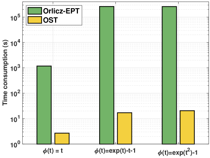
Figure 4: Time consumption on graph ${\mathbb{G}}_{\text{Log}}$.

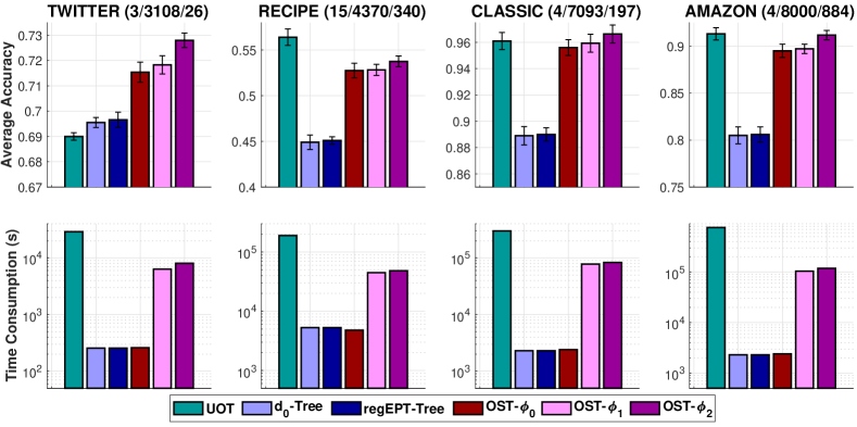
Figure 5: Document classification on graph ${\mathbb{G}}_{\text{Log}}$.

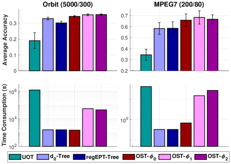
Figure 6: TDA on graph ${\mathbb{G}}_{\text{Log}}$.

References

• Adams et al. (2017) Adams, H., Emerson, T., Kirby, M., Neville, R., Peterson, C., Shipman, P., Chepushtanova, S., Hanson, E., Motta, F., and Ziegelmeier, L. Persistence images: A stable vector representation of persistent homology. Journal of Machine Learning Research, 18(1):218–252, 2017.
• Adams & Fournier (2003) Adams, R. A. and Fournier, J. J. Sobolev spaces. Elsevier, 2003.
• Altschuler & Chewi (2023) Altschuler, J. M. and Chewi, S. Faster high-accuracy log-concave sampling via algorithmic warm starts. arXiv preprint arXiv:2302.10249, 2023.
• Andoni et al. (2018) Andoni, A., Lin, C., Sheng, Y., Zhong, P., and Zhong, R. Subspace embedding and linear regression with Orlicz norm. In International Conference on Machine Learning, pp. 224–233. PMLR, 2018.
• Balaji et al. (2020) Balaji, Y., Chellappa, R., and Feizi, S. Robust optimal transport with applications in generative modeling and domain adaptation. Advances in Neural Information Processing Systems, 33:12934–12944, 2020.
• Benamou (2003) Benamou, J.-D. Numerical resolution of an “unbalanced” mass transport problem. ESAIM: Mathematical Modelling and Numerical Analysis-Modélisation Mathématique et Analyse Numérique, 37(5):851–868, 2003.
• Bonneel & Coeurjolly (2019) Bonneel, N. and Coeurjolly, D. Spot: sliced partial optimal transport. ACM Transactions on Graphics (TOG), 38(4):1–13, 2019.
• Bonneel et al. (2015) Bonneel, N., Rabin, J., Peyré, G., and Pfister, H. Sliced and radon wasserstein barycenters of measures. Journal of Mathematical Imaging and Vision, 51(1):22–45, 2015.
• Caffarelli & McCann (2010) Caffarelli, L. A. and McCann, R. J. Free boundaries in optimal transport and Monge-Ampere obstacle problems. Annals of mathematics, pp.  673–730, 2010.
• Chamakh et al. (2020) Chamakh, L., Gobet, E., and Szabó, Z. Orlicz random Fourier features. The Journal of Machine Learning Research, 21(1):5739–5775, 2020.
• Chapel et al. (2020) Chapel, L., Alaya, M. Z., and Gasso, G. Partial optimal tranport with applications on positive-unlabeled learning. Advances in Neural Information Processing Systems, 33:2903–2913, 2020.
• Chewi (2023) Chewi, S. An optimization perspective on log-concave sampling and beyond. PhD thesis, Massachusetts Institute of Technology, 2023.
• Chizat et al. (2018) Chizat, L., Peyré, G., Schmitzer, B., and Vialard, F.-X. Unbalanced optimal transport: Dynamic and Kantorovich formulations. Journal of Functional Analysis, 274(11):3090–3123, 2018.
• Cover & Thomas (1999) Cover, T. M. and Thomas, J. A. Elements of information theory. John Wiley & Sons, 1999.
• Cuturi (2013) Cuturi, M. Sinkhorn distances: Lightspeed computation of optimal transport. In Advances in Neural Information Processing Systems, pp. 2292–2300, 2013.
• Deng et al. (2022) Deng, Y., Song, Z., Weinstein, O., and Zhang, R. Fast distance oracles for any symmetric norm. Advances in Neural Information Processing Systems, 35:7304–7317, 2022.
• Edelsbrunner & Harer (2008) Edelsbrunner, H. and Harer, J. Persistent homology-a survey. Contemporary mathematics, 453:257–282, 2008.
• Figalli (2010) Figalli, A. The optimal partial transport problem. Archive for rational mechanics and analysis, 195(2):533–560, 2010.
• Frogner et al. (2015) Frogner, C., Zhang, C., Mobahi, H., Araya, M., and Poggio, T. A. Learning with a wasserstein loss. In Advances in neural information processing systems, pp. 2053–2061, 2015.
• Gangbo et al. (2019) Gangbo, W., Li, W., Osher, S., and Puthawala, M. Unnormalized optimal transport. Journal of Computational Physics, 399:108940, 2019.
• Guha et al. (2023) Guha, A., Ho, N., and Nguyen, X. On excess mass behavior in Gaussian mixture models with Orlicz-Wasserstein distances. In International Conference on Machine Learning, ICML, volume 202, pp.  11847–11870. PMLR, 2023.
• Guittet (2002) Guittet, K. Extended Kantorovich norms: a tool for optimization. INRIA report, 2002.
• Hanin (1992) Hanin, L. G. Kantorovich-Rubinstein norm and its application in the theory of Lipschitz spaces. Proceedings of the American Mathematical Society, 115(2):345–352, 1992.
• Kell (2017) Kell, M. On interpolation and curvature via Wasserstein geodesics. Advances in Calculus of Variations, 10(2):125–167, 2017.
• Kondratyev et al. (2016) Kondratyev, S., Monsaingeon, L., and Vorotnikov, D. A new optimal transport distance on the space of finite Radon measures. Advances in Differential Equations, 21(11/12):1117–1164, 2016.
• Latecki et al. (2000) Latecki, L. J., Lakamper, R., and Eckhardt, T. Shape descriptors for non-rigid shapes with a single closed contour. In Proceedings of the IEEE Conference on Computer Vision and Pattern Recognition (CVPR), volume 1, pp.  424–429, 2000.
• Le & Nguyen (2021) Le, T. and Nguyen, T. Entropy partial transport with tree metrics: Theory and practice. In Proceedings of The 24th International Conference on Artificial Intelligence and Statistics (AISTATS), volume 130 of Proceedings of Machine Learning Research, pp.  3835–3843. PMLR, 2021.
• Le et al. (2022) Le, T., Nguyen, T., Phung, D., and Nguyen, V. A. Sobolev transport: A scalable metric for probability measures with graph metrics. In International Conference on Artificial Intelligence and Statistics, pp.  9844–9868. PMLR, 2022.
• Le et al. (2023) Le, T., Nguyen, T., and Fukumizu, K. Scalable unbalanced Sobolev transport for measures on a graph. In International Conference on Artificial Intelligence and Statistics, pp.  8521–8560. PMLR, 2023.
• Le et al. (2024) Le, T., Nguyen, T., and Fukumizu, K. Generalized Sobolev transport for probability measures on a graph. In Forty-first International Conference on Machine Learning, 2024.
• Lellmann et al. (2014) Lellmann, J., Lorenz, D. A., Schonlieb, C., and Valkonen, T. Imaging with Kantorovich–Rubinstein discrepancy. SIAM Journal on Imaging Sciences, 7(4):2833–2859, 2014.
• Liero et al. (2018) Liero, M., Mielke, A., and Savaré, G. Optimal entropy-transport problems and a new Hellinger–Kantorovich distance between positive measures. Inventiones mathematicae, 211(3):969–1117, 2018.
• Lorenz & Mahler (2022) Lorenz, D. and Mahler, H. Orlicz space regularization of continuous optimal transport problems. Applied Mathematics & Optimization, 85(2):14, 2022.
• Mikolov et al. (2013) Mikolov, T., Sutskever, I., Chen, K., Corrado, G. S., and Dean, J. Distributed representations of words and phrases and their compositionality. In Advances in neural information processing systems, pp. 3111–3119, 2013.
• Mukherjee et al. (2021) Mukherjee, D., Guha, A., Solomon, J. M., Sun, Y., and Yurochkin, M. Outlier-robust optimal transport. In International Conference on Machine Learning, pp. 7850–7860. PMLR, 2021.
• Müller (1997) Müller, A. Integral probability metrics and their generating classes of functions. Advances in Applied Probability, 29(2):429–443, 1997.
• Musielak (2006) Musielak, J. Orlicz spaces and modular spaces, volume 1034. Springer, 2006.
• Nguyen et al. (2023) Nguyen, Q. M., Nguyen, H. H., Zhou, Y., and Nguyen, L. M. On unbalanced optimal transport: Gradient methods, sparsity and approximation error. The Journal of Machine Learning Research, 2023.
• Pham et al. (2020) Pham, K., Le, K., Ho, N., Pham, T., and Bui, H. On unbalanced optimal transport: An analysis of Sinkhorn algorithm. In Proceedings of the International Conference on Machine Learning, 2020.
• Piccoli & Rossi (2014) Piccoli, B. and Rossi, F. Generalized Wasserstein distance and its application to transport equations with source. Archive for Rational Mechanics and Analysis, 211(1):335–358, 2014.
• Piccoli & Rossi (2016) Piccoli, B. and Rossi, F. On properties of the generalized Wasserstein distance. Archive for Rational Mechanics and Analysis, 222(3):1339–1365, 2016.
• Rao & Ren (1991) Rao, M. M. and Ren, Z. D. Theory of Orlicz spaces. Marcel Dekker, 1991.
• Sato et al. (2020) Sato, R., Yamada, M., and Kashima, H. Fast unbalanced optimal transport on tree. In Advances in neural information processing systems, 2020.
• Séjourné et al. (2019) Séjourné, T., Feydy, J., Vialard, F.-X., Trouvé, A., and Peyré, G. Sinkhorn divergences for unbalanced optimal transport. arXiv preprint arXiv:1910.12958, 2019.
• Séjourné et al. (2022) Séjourné, T., Vialard, F.-X., and Peyré, G. Faster unbalanced optimal transport: Translation invariant sinkhorn and 1-d frank-wolfe. In Proceedings of The 25th International Conference on Artificial Intelligence and Statistics, volume 151, pp.  4995–5021. PMLR, 2022.
• Song et al. (2019) Song, Z., Wang, R., Yang, L., Zhang, H., and Zhong, P. Efficient symmetric norm regression via linear sketching. Advances in Neural Information Processing Systems, 32, 2019.
• Sturm (2011) Sturm, K.-T. Generalized Orlicz spaces and Wasserstein distances for convex–concave scale functions. Bulletin des sciences mathématiques, 135(6-7):795–802, 2011.
Supplement to “Sobolev-Orlicz Transport for Unbalanced Measures on a Graph”
In this appendix, we describe detailed proofs in §A. Further results and discussions are placed in §B.
Notations.
The indicator function $\bf{1}$ of a set $X$ is defined as follows:
$${\bf{1}}_{X}(x)=\begin{cases}1&\text{if }x\in X\\ 0&\text{otherwise}.\end{cases}$$ (23)